Chapter 7

Graphics

Bringing visual expression to the web.

Introduction

In computer graphics, we have two primary approaches to representing graphical information, raster and vector representations.

Raster graphics take their name from the scan pattern of a cathode-ray tube, such as was used in older television sets and computer monitors. These, as well as modern monitors, rely on a regular grid of pixels composed of three colors of light (red, green, and blue) that are mixed at different intensities to create all colors of the visible spectrum.

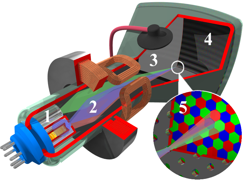
A cathode ray tube cutwaway diagram with numbered parts. — Cathode Ray Tube
A cathode ray tube (CRT) screen works by firing electrons out of an electron gun (1) through electromagnetic coils (2) that steer them through a perforated mask (3) that separates the electrons corresponding to the red, green, and blue components of an individual pixels. These electrons then strike the phosphor-coated back of the screen (4), causing it to emit photons of a particular wavelength.Image courtesy of Søren Peo Pedersen, made available through the creative commons share-alike 3.0 license.

This inheritance from CRT monitors is important, because it affects several details about how computer graphics are implemented. Because CRT screens blend three colors of light (red, green, and blue) at different intensities, they needed to be supplied these intensities, and they needed to be grouped together into single pixels, as the electron gun can only light up a single cluster of phosphorus dots at once. The illusion of a continuous image is generated because the electron beam scans across the back of the screen so rapidly that the pixels appear to be constantly lit.

The scanning pattern the electron beam takes begins at the upper left corner of the screen, and sweeps from left to right. When the right edge of the screen is reached, then the beam drops to the next row, and again scans left to right. This continues until the lower right corner is reached, at which point the beam begins back in the upper left-hand corner - just like reading a book in the English language. CRT screens were first used in analog televisions, which receive a continuous signal that streams pixel intensities, so this made a lot of sense to the engineers designing them. When computers first started needing monitors, the existing CRT technology was adapted to fit them - as a result, in computer graphics, the origin is in the upper left corner of the screen, and the y-axis increases in a downward direction:

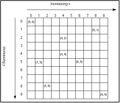
Screen/Computer graphics coordinate system — Image taken from inetjava.sourceforge.net and believed to be public domain.

Warning

The origin being located in the upper-left corner and the Y-axis increasing in a downward direction sometimes confuses novice programmers, who expect the origin to be in the lower right corner and the y-axis to increase in an upward direction, as is the case in Euclidean geometry .

Additionally, early computers needed a location to store what should be displayed on the screen, which the computer’s VGA card could then continuously stream from to correctly display on-screen. This video memory consisted of a linear array of pixel data - each pixel was typically represented by three eight-bit numbers corresponding to the intensity of the red, green, and blue for each pixel. Thus, each intensity would range from 0 (fully off) to 255 (fully on; remember, $2^8 = 256$). This was, in the early days of computers, quite memory-consumptive (a VGA monitor would use 640 x 489 x 3 bytes, or 900 kilobytes to hold the screen’s data), so many early graphics cards supported alternative graphics modes used a color lookup table and kept corresponding indices in the linear array. While this is no longer common in modern computer equipment, some simple embedded systems still utilize these kinds of video modes.

Raster Graphic Files

Unsurprisingly, graphic files that store their data in a raster format borrow heavily from the representations discussed previously . Typically, a graphic file consists of two parts, a head and a body. This is very much like how the <head> of a HTML file provides metadata about the page and the <body> contains the actual page contents. For a raster graphic file, the head of the file contains metadata describing the image itself - the color format, along with the width and height of the image. The body contains the actual raster data, in a linear array much like that used by the computer screen.

This data may be compressed, depending on the file format used. Some compression algorithms, like the one used in JPEG files, are lossy (that is, they “lose” some of the fine detail of the image as a side-effect of the compression algorithm). Tagged image file format (tiff), bitmaps (bmp), and portable network graphics (png) are popular formats for the web with the latter (png) especially suitable for websites.

The origin of a raster graphic file is also in the upper left corner, and the raster data is typically comprised of three or four eight-bit color channels corresponding to Red, Green, Blue, and Alpha (the alpha channel is typically used to represent the opacity of the pixel, with 255 being completely solid and 0 being completely transparent). Because the raster data for video memory and for raster graphic files are ordered in the same way, putting a raster graphic on-screen simply requires copying the pixel data from one linear array into the other - a relatively fast process (Computer scientists would describe it as having a complexity of $O(n)$).

HTML Raster Graphics

The most obvious use of raster graphics in HTML is the <img> element, a HTML element that embodies a single raster graphic image. It is defined with the an img tag:

<img src="" alt="">

The src attribute is a relative or absolute url of an image file, and the alt attribute provides a textual description of what the image portrays. It is what the browser displays if the image file does not load, and is also important for screen readers (as discussed in Chapter 6 ).

Any HTML element can also be given a raster graphic to use as a background through the CSS background-image property:

background-image(url([route/to/file]));

The url() function converts a relative or absolute path ([route/to/file]) for the browser to retrieve with a HTTP request (relative paths are relative to the file containing the rule declaration). By default, the image will have its origin in the upper left corner of the HTML element the rule is applied to, and will extend pixel-by-pixel until the edge of the containing element is reached (this means that to display the full image, you may need to set the width and height attributes for the element as well). If the image is smaller than the containing element, it will be tiled. Tiling can be conditionally turned off through the background-repeat property, in the X, Y, or both axes. You can also stretch, crop, and shift the image’s origin with other background properties.

In addition to these two strategies for including graphics in a web site, HTML provides a third option in the <canvas> element. We’ll discuss that next.

The Canvas Element

The <canvas> element represents a raster graphic, much like the <img> element. But instead of representing an existing image file, the <canvas> is a blank slate - a grid of pixels on which you can draw using JavaScript. Becuase a canvas doesn’t determine its size from an image file, you need to always declare it with a width and height attribute (otherwise, it has a width and height of 0):

<div style="border 1px solid gray">
  <canvas id="example-canvas-1" width=400 height=200></canvas>
  <button onclick="fillCanvas">Fill Canvas<button>
  <button onclick="clearCanvas">Clear Canvas</button>
</div>

You probably noticed that there appears to be nothing on the page above - but our canvas is there, it is just empty! Clicking the Fill button will fill it with a solid color, and the Clear button will erase it. So how does this work?

To draw into a canvas, we also need a context, a JavaScript object that allows us to draw onto the canvas. We’ll specifically be using the CanvasRenderingContext2D. To get one, we:

Get a reference to the canvas object
Call its getContext() method with an argument of '2d'

The JavaScript to do so looks like:

var canvas = document.getElementById('example-canvas-1');
var ctx = canvas.getContext('2d');

Once we have the context, we can draw onto the canvas using one of its many commands

function fillCanvas() {
  ctx.fillRect(0, 0, 200, 400);
}

The result can be seen in the canvas above. Next, let’s discuss how the canvas element and context work together.

The Pen Metaphor

Most 2D graphics libraries adopt a “pen” metaphor to model how they interact with the graphics they draw. Think of an imaginary pen that you use to draw on the screen. When you put the pen down and move it across the screen you draw a line - the stroke. When you lift the pen, you no longer make a mark. The movements of the pen across the canvas also define a path.

There are a number of methods that move this imaginary pen:

moveTo(x, y) picks up the imaginary pen and puts it back down at the position specified by x and y).
lineTo(x, y) moves the imaginary pen across the canvas, drawing a line from its prior position to the position specified by x and y.
bezierCurveTo(c1x, c1y, c2x, c2y, x, y) moves the imaginary pen across the canvas following a Bezier curve defined by the starting point, control points (c1x, c1y), (c2x, c2y), and ending point (x, y).
arc(x, y, radius, startAngle, endAngle) draws an arc (a segment of a circle) centered at (x,y) with radius radius and starting at startAngle and ending at endAngle (both measured in radians with the positive x-axis representing 0 radians). An optional final boolean parameter counterclockwise draws the arc counterclockwise instead of clockwise when true.
arcTo(x, y, radius, startAngle, endAngle) works as the arc() method, but it picks up the pen.

It is important to understand that the path defined by these methods does get drawn into the canvas until one or both of the context’s stroke() or fill() functions is called. These methods apply to the current path of the pen - we can also begin a new path with the beginPath() function, which clears all of the previous path. We can also make the path return to its starting point with the closePath() function.

We’ll discuss stroke and fill next, but for now, here is an example of a canvas using the ideas we just discussed:

<canvas id="example" width="500" height="300"></canvas>
<script>
  var canvas = document.getElementById('example');
  var ctx = canvas.getContext('2d');
  
  ctx.beginPath();
  ctx.moveTo(100, 100);
  ctx.lineTo(100, 200);
  ctx.bezierCurveTo(100, 300, 300, 300, 300, 200);
  ctx.arc(300, 200, 100, 0, Math.PI, true);
  ctx.stroke();
</script>

Stroke and Fill

The stroke and fill work with the current path of the context, defining how the outline and interior of a shape defined by the path are drawn.

Stroke

The stroke() draws all of the path segments where the pen was “down”. The appearance of the stroke can be altered with specific properties of the canvas:

strokeStyle allows you to set the color of the stroke, i.e. ctx.strokeStyle = 'orange';. You can use one of the named colors, i.e. 'green', a hexidecimal value, i.e. #fafafa, one of the color functions rgb(233,23,155), rgba(23,23,23, 0.4), or a gradient or pattern (see more detail in the MDN web docs ).
lineWidth allows you to set the width of the drawn line, in coordinate units (pixels of the canvas), i.e. ctx.lineWidth = 3.0;
lineCap defines what the end of a line looks like, "Butt" for a squared-off end, "round" for a rounded end, or "square" for a box with width and height equal to the line’s thickness, centered on the end.
lineDashOffset adds an offset to the first dash in a dashed line. See the discussion of dashed lines below.

Lines can also be dashed. The nature of the dash is set wit the setLineDash(segmentArray) function of the context. The segmentArray is an array of distances which indicate the length of alternating lines and gaps forming the dash. For example:

ctx.setLineDash([5, 4]);

Creates a dash pattern of 5 units of line followed by 4 units of space. Then the pattern repeats, so another 5 units of line, and so on.

Let’s redraw our previous shape with some changes to our stroke:

<canvas id="example" width="500" height="300"></canvas>
<script>
  var canvas = document.getElementById('example');
  var ctx = canvas.getContext('2d');
  ctx.strokeStyle = 'green';
  ctx.beginPath();
  ctx.moveTo(100, 100);
  ctx.lineTo(100, 200);
  ctx.bezierCurveTo(100, 300, 300, 300, 300, 200);
  ctx.stroke();
  // begin a new path so a different line style is applied
  ctx.beginPath();
  ctx.strokeStyle = 'blue';
  ctx.setLineDash([5,2,1,2]);
  ctx.arc(300, 200, 100, 0, Math.PI, true);
  ctx.closePath();
  ctx.stroke();
</script>

Info

Note how we added a beginPath() to change the line style, and also how that altered the behavior of the closePath() function (instead of closing with the original point of the first path, it closes with the first point of the second path). When drawing complex shapes, you’ll need to pay careful attention to your subpaths.

Fill

The fill() function fills in the shape outlined by the path (both the parts where the pen was “down” and also “up”). The appearance of the fill can also be altered with the fillStyle property of the canvas.

The fillStyle property allows you to change the color of the fill with one of several possible values: color i.e. ctx.fillStyle='purple';. It can use named colors (i.e. 'green'), hexidecimal values (i.e. #ffffdd), one of the color functions (i.e. rgb(0.4, 0.4. 0.9)), a gradient, which can be linear, conic, or radial, or a pattern, such as repeating images. You can find more about using each in the MDN web docs .

<canvas id="example-2" width="500" height="300"></canvas>
<script>
  var canvas2 = document.getElementById('example-2');
  var ctx2 = canvas2.getContext('2d');
  ctx2.fillStyle = 'purple';
  ctx2.moveTo(100, 100);
  ctx2.lineTo(100, 200);
  ctx2.bezierCurveTo(100, 300, 300, 300, 300, 200);
  ctx2.arc(300, 200, 100, 0, Math.PI, true);
  ctx2.closePath();
  ctx2.fill();
</script>

Shape Functions

For ease of use, the context also supplies a number of functions for drawing shapes. Some of these just define the shape as a series of subpaths to be used with the stroke() and fill() functions.

Arcs and Circles

Of these, we’ve already seen the arc(x, y, radius, startAngle, endAngle) function. It can be used to draw an arc, or when filled, a wedge - like a pie slice. When a startAngle of 0 and endAngle of 2 * Math.PI is used, it instead draws a complete circle.

<canvas id="arc-example" width="500" height="200"></canvas>
<script>
  var canvas = document.getElementById('arc-example');
  var ctx = canvas.getContext('2d');
  
  ctx.strokeStyle = 'green';
  ctx.arc(100, 100, 50, 0, Math.PI * 2);
  ctx.stroke();
  
  ctx.beginPath();
  ctx.fillStyle = 'purple';
  ctx.arc(250, 100, 50, 0, Math.PI * 2);
  ctx.fill();

  ctx.beginPath();
  ctx.moveTo(400, 100);
  ctx.arc(400, 100, 50, Math.PI, Math.PI / 4);
  ctx.stroke();
  ctx.fill();
</script>

Ellipse

There is also an ellipse(x, y, radiusX, radiusY, startAngle, endAngle) function. It works in a similar way, creating an ellipse centered on the point (x, y) with a horizontal radius of radiusX and a vertical radius of radiusY, and starting and ending angles of startAngle and endAngle (specified in radians). As with the arc() method, a startAngle of 0 and endAngle of 2 * Math.PI creates a full ellipse.

Rectangle

The rect(x, y, width, height) function draws a rectangle with upper left corner at (x, y) and dimensions width and height. In addition to the rect() function, there are some shorthand functions that also stroke or fill the rect without altering the current path.

The first of these is fillRect(x, y, width, height) which uses the same arguments as rect() and fills the resulting rectangle with the current fill style. We used this in the introduction .

The second is the clearRect(x, y, width, height) function, which fills the rect defined by the arguments with transparent black (rgba(0,0,0,0)), effectively erasing everything in that rectangle on the canvas.

Info

Why the extra rectangle shorthands, and not other shapes? Remember, computer graphics have traditionally been rectangular, i.e. windows are rectangles. So programmers have gotten used to using rectangles in a lot of places, so having the extra shorthands made sense to the developers. Also, both fillRect() and clearRect() are used to quickly clear <canvas> elements of any prior drawing, especially when creating canvas animations.

Canvas Text

While the canvas is primarily used to draw graphics, there are times we want to use text as well. We have two methods to draw text: fillText(text, x, y) and strokeText(text, x, y). The text parameter is the text to render, and the x and y are the upper left corner of the text.

As with the fillRect() and strokeRect() functions, fillText() and strokeText() fill and stroke the text, respectively, and the text does not affect the current path. The text properties are set by properties on the context:

font is the font to use for the text. It uses the same syntax as the CSS font property. I.e. ctx.font = 10pt Arial;
textAlign sets the alignment of the text. Possible values are start, end, left, right, or center.
textBaseline sets the baseline alignment for the text. Possible values are top, hanging, middle, alphabetic, ideographic, or bottom.
direction the directionality of the text. Possible values are ltr (left-to-right), rtl (right-to-left), and inherit (inherit from the page settings).

<canvas id="example" width="500" height="300"></canvas>
<script>
  var canvas = document.getElementById('example');
  var ctx = canvas.getContext('2d');
  
  ctx.font = "40pt symbol";
  ctx.strokeText("Foo", 100, 100);
  ctx.fillText("Bar", 100, 200);
</script>

Info

Sometimes you might want to know how large the text will be rendered in the canvas. The measureText(text) function returns a TextMetrics object describing the size of a rectangle that the supplied text would fill, given the current canvas text properties.

Canvas and Images

The <canvas> and <img> elements are both raster representations of graphics, which introduces an interesting possibility - copying the data of an image into the canvas. This can be done with the drawImage() family of functions.

The first of these is drawImage(image, x, y). This copies the entire image held in the image variable onto the canvas, starting at (x, y).

<canvas id="image-example-1" width="500" height="300"></canvas>
<script>
  var canvas1 = document.getElementById('image-example-1');
  var ctx1 = canvas1.getContext('2d');
  var image1 = new Image();
  image1.onload = function() {
    ctx1.drawImage(image1, 0, 0);
  }
  image1.src = "/cc120/images/rubber_duck_debugging.jpg";  
</script>

The second, drawImage(image, x, y, width, height) scales the image as it draws it. Again the image is drawn starting at (x,y) but is scaled to be width x height.

<canvas id="image-example-2" width="500" height="300"></canvas>
<script>
  var canvas2 = document.getElementById('image-example-2');
  var ctx2 = canvas2.getContext('2d');
  var image2 = new Image();
  image2.onload = function() {
    ctx2.drawImage(image2, 0, 0, 300, 300);
  }
  image2.src = "/cc120/images/rubber_duck_debugging.jpg";  
</script>

The third, drawImage(image, sx, sy, sWidth, sHeight, x, y, width, height) draws a sub-rectangle of the source image. The source sub-rectangle starts at point (sx, sy) and has dimensions sWidth x sHeight. It draws the contents of the source rectangle into a rectangle in the canvas starting at (dx,dy) and scaled to dimensions dWidth x dHeight.

<canvas id="image-example-3" width="500" height="300"></canvas>
<script>
  var canvas3 = document.getElementById('image-example-3');
  var ctx3 = canvas3.getContext('2d');
  var image3 = new Image();
  image3.onload = function() {
    ctx3.drawImage(image3, 200, 200, 300, 300, 0, 0, 300, 300);
  }
  image3.src = "/cc120/images/rubber_duck_debugging.jpg";  
</script>

Warning

If the image is not loaded when the drawImage() call is made, nothing will be drawn to the canvas. This is why in the examples, we move the drawImage() call into the onload callback of the image - this function will only be invoked when the image finishes loading.

Tip

Because a <canvas> element is itself a grid of pixels just like an <img> element, you can also use a <canvas> in a drawImage() call! This can be used to implement double-buffering, a technique where you draw the entire scene into a <canvas> element that is not shown in the webpage (known as the back buffer), and then copying the completed scene into the on-screen <canvas> (the front buffer).

Transforms and State

Much like we can use CSS to apply transformations to HTML elements, we can use transforms to change how we draw into a canvas. The rendering context has a transformation matrix much like those we discussed in the CSS chapter, and it applies this transform to any point it is tasked with drawing.

We can replace the current transformation matrix with the setTransform() function, or multiply it by a new transformation (effectively combining the current transformation with the new one) by calling transform().

With this in mind, it can be useful to know two other functions of the context, save() and restore(). These save the current context state by pushing and popping from a stack. Think of it as a pile of papers. When we call save() we write down the current state of the context object, and drop that paper in the stack. When we call restore(), we take the topmost paper from the stack, and set context’s state back to what was written on that sheet.

So what exactly constitutes the state of our rendering context? As you might imagine, this includes the transformation matrix we just talked about. But it also includes all of the stroke and fill properties.

Now, back to the transforms. As with CSS transforms, we can define the matrix ourselves, but there also exist a number of helper functions we can leverage, specifically:

translate(tx, ty) translates by tx in the x axis, and ty along the y
rotate(angle) rotates around the z-axis by the supplied angle (specified in radians)
scale(sx,sy) scales by sx along the x axis, and sy along the y axis. This is expressed as a decimal value: 1.0 indicates 100%, 0.5 for 50%, and 1.75 for 175%

<canvas id="example" width="500" height="300"></canvas>
<script>
  var canvas = document.getElementById('example');
  var ctx = canvas.getContext('2d');
  
  ctx.font = "40pt Tahoma";
  var metrics = ctx.measureText("Hello Canvas");
  var tx = 100 + metrics.width / 2;
  var ty = 180;
  
  ctx.translate(tx, ty);
  ctx.rotate(Math.PI/4);
  ctx.translate(-tx, -ty);

  ctx.strokeText("Hello Canvas", 100, 180);
</script>

Info

In this example, we translate the text so that its center is at the origin before we rotate it, then translate it back. As any rotation we specify is around the origin, this makes it so the text is rotated around its center and stays on canvas, rather than rotating off the canvas.

Also notice that we call the transformation functions in the opposite order we want them applied.

Animation

The canvas element provides a powerful tool for creating animations by allowing us to erase and re-draw its contents over and over. Ideally, we only want to redraw the canvas contents only as quickly as the screen is updated (typically every 1/30th or 1/60th of a second). The window.requestAnimationFrame(callback) provides an approach for doing this - it triggers the supplied callback every time the monitor refreshes.

Inside that callback, we want to erase the canvas and then draw the updated scene. Here is an example animating a ball bouncing around the canvas:

<canvas id="example" width="500" height="300"></canvas>
<script>
  var canvas = document.getElementById('example');
  var ctx = canvas.getContext('2d');
  var x = 100;
  var y = 100;
  var dx = Math.random();
  var dy = Math.random();
  
  function animate(timestamp)
  {
    ctx.fillStyle = 'pink';
    ctx.fillRect(0,0,500,300);
    ctx.fillStyle = 'blue';
    ctx.beginPath();
    ctx.arc(x, y, 25, 0, 2*Math.PI);
    ctx.fill();
    ctx.stroke();
    x += dx;
    y += dy;
    if(x < 25 || x > 475) dx = -dx;
    if(y < 25 || y > 275) dy = -dy;
    window.requestAnimationFrame(animate);
  }

  animate();

</script>

Info

On monitors with different refresh rates, the ball will move at a different speed. The callback function supplied to requestAnimationFrame() will receive a high-resolution timestamp (the current system time). You can save the previous timestamp and subtract it from the current time to determine how much time elapsed between frames, and use this to calculate your animations. An example doing this can be found in the MDN web docs .

Vector Graphics

Up to this point, we’ve been discussing raster graphics, which are represented by a grid of pixels. In contrast, vector graphics are stored as a series of instructions to re-create the graphic. For most vector approaches, these instructions look similar to those we issued to our JavaScript rendering context when working with the <canvas> element - including the idea of paths, stroke, and fill.

The vector approach has its own benefits and drawbacks when compared to raster graphics.

More Computation Before a vector graphic can be displayed, it has to be rendered into a raster form, much like we had to instruct our context to render into a <canvas>. This requires some computation, whereas rendering a raster graphic simply requires copying its bits from one buffer to another (assuming we aren’t scaling it).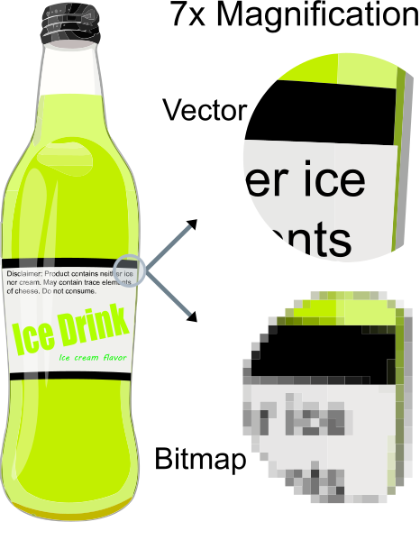
Better Scaling Perhaps the biggest benefit is that the problems we see when scaling a raster graphic don’t happen with vector graphics. If we want to make the graphic ten times larger, then when we convert it into a raster, we can scale up the drawing instructions to ten times the normal size.
Less Photorealistic Vector graphics are best suited for images with well-defined shapes with little shading - things like clipart and cartoon characters. To approach photorealism requires a lot of small shapes drawn in different colors, and will require both more memory and computation. In contrast, a raster graphic is excellent at photorealism. Digital cameras actually create a raster graphic from a grid of color sensors behind the lens.

Because of the scaling benefits, vector graphics are used for commonly used for fonts, icons, and logos, and other images that may be presented at vastly different scales.

SVG

The Scalable Vector Graphics (SVG) image format is a file format for creating a vector graphic. It uses the same ideas about path, stroke, and fill and coordinate that we discussed with the canvas. It also is a text format based on XML, as was HTML. So the contents of a XML file will look familiar to you. Here is an example:

<svg viewBox="0 0 500 200" xmlns="http://www.w3.org/2000/svg">
  <path d="M 100 50 L 100 150 L 300 150 Z" stroke="black" fill="#dd3333"/>
</svg>

Let’s take a close look at the file format. First, like HTML and other XML derivatives, we use tags to specify elements. The <svg> tag indicates the top level of our SVG image, much like the <html> tag does for HTML. The xmlns links to the specification of the XML format, and should be included in all <svg> elements (it’s one of the requirements of the XML format - earlier versions of HTML did this as well for the HTML namespace, but HTML5 broke away from the requirement).

Likewise the <path> element defines a path, much like those we drew with the <canvas> and its rendering context. The d attribute in the <path> is its data, and it provides it a series of commands and values, separated by spaces. These instruct the program rendering the SVG in how to move the imaginary pen around. The stroke and fill attributes specify how the resulting path should be stroked and filled.

Finally, the viewBox attribute in the <svg> tag describes what part of the image should be rendered. This is specified as a rectangle, following the familiar format of x y width height, where the point (x,y) is the upper left corner, and width and height specify a distance to the left and down, respectively.

The viewBox plays an important role in how SVG graphics scale. If we used this SVG in an <img> tag and set it to have a different width, it would automatically scale the view box contents to match:

<img src="/images/triangle.svg" width="200">

Now that you understand the basics, let’s turn our attention to some specific SVG elements.

Info

There is an important idea in the above discussion - the SVG file format specifies how the image should be drawn. But it is up to the program reading the SVG to actually carry out the drawing commands. As this is much more involved than simply copying raster bits, not all image viewing software support SVG files. However, all modern browsers do.

SVG Paths

SVGs use the same pen metaphor we saw with the <canvas> and one of the most basic approaches to drawing in an SVG is the <path> element. Each <path> should contain a d attribute, which holds the commands used to draw the path. These are very similar to the commands we used with the <canvas> and the CanvasRenderingContext2D we used earlier, but instead of being written as a function call, they are written as a capital letter (indicating what command to carry out) followed by numbers specifying the action. Let’s take another look at our earlier example:

The path’s data is M 100 50 L 100 150 L 300 150 Z. Let’s break it down one command at a time:

M 100 50 indicates we should move our pen to point (100, 50).
L 100 150 indicates we should draw a line from our current position to point (100, 150).
L 300 150 indicates we should draw a line from our current position to point (300, 150).
Z indicates we should close our path, drawing a line to where we started (the point specified in our first command).

Now that we’ve worked through a path example, let’s discuss the specific commands available to us:

Move To

The M x y command indicates we should move to the point (x, y), picking up our pen. It corresponds to ctx.moveTo(x, y).

Line To

The L x y command indicates we should draw a line from our current position to the point (x, y). It corresponds to ctx.lineTo(x, y).

Horizontal Line To

The H x command is shorthand for drawing a horizontal line (the y stays the same) from the current x to the provided x.

Vertical Line To

The V y command is shorthand for drawing a vertical line (the x stays the same) from the current y to the provided y.

Curve To

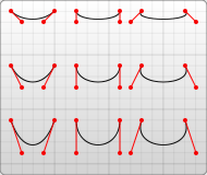
The C cx1 cy1, cx2 cy2, dx, dy is the shorthand for drawing a Bézier Curve from the current position to (dx, dy) using control points (cx1, cy1) and (cx2, cy2). It corresponds to ctx.curveTo(c1x, c1y, c2x, c2y, dx, dy). The MDN web docs has an excellent discussion with visual examples of Bézier curves . A visual example of the role of the effect control points have on a Bézier curve from that article appears below:

Arc To

The A rx ry x-axis-rotation large-arc-flag sweep-flag x y a rx ry x-axis-rotation large-arc-flag sweep-flag dx dy draws an arc. It is roughly analogous to the ctx.drawArc() method, but uses a different way of specifying the arc’s start, end, and direction. You can read a more detailed discussion on the MDN Web Docs

Info

The examples on this page have been adapted from the MDN web docs . You are encouraged to visit these documents for a much more detailed discussion of the concepts and techniques presented here.

SVG Shapes

Much like the CanvasRenderingContext2d we used with the <canvas> earlier allowed us to render rectangles outside of the path, the SVG format also provides mechanisms for rendering common shapes. These are specified using their own tags (like HTML elements), and there are a wide variety of shapes available:

Rectangle

The <rect> element defines a rectangle, specified by the now-familiar x, y,, width and height attributes, and with optional rounded corners with radius specified by the rx attribute.

<svg viewBox="0 0 220 100" xmlns="http://www.w3.org/2000/svg" height="200">
  <!-- Simple rectangle -->
  <rect width="100" height="100" fill="cornflowerblue"/>

  <!-- Rounded corner rectangle -->
  <rect x="120" width="100" height="100" rx="15" fill="goldenrod"/>
</svg>

Circle

The <circle> elements defines a circle with radius and center defined by the r, cx, and cy attributes:

<svg viewBox="0 0 100 100" xmlns="http://www.w3.org/2000/svg">
  <circle cx="50" cy="50" r="50" fill="cornflowerblue"/>
</svg>

Ellipse

The <ellipse> element represents an ellipse, with center (cx, cy) horizontal radius (rx) and vertical radius (ry) specified by the corresponding attributes:

<svg viewBox="0 0 200 100" xmlns="http://www.w3.org/2000/svg" height="200">
  <ellipse cx="100" cy="50" rx="100" ry="50" fill="goldenrod"/>
</svg>

Polygon

The <polygon> specifies an arbitrary polygon using a series of points defined by the points attribute:

<svg viewBox="0 0 200 100" xmlns="http://www.w3.org/2000/svg" height="200">
  <!-- Example of a polygon with the default fill -->
  <polygon points="0,100 50,25 50,75 100,0" fill="magenta"/>

  <!-- Example of the same polygon shape with stroke and no fill -->
  <polygon points="100,100 150,25 150,75 200,0" fill="none" stroke="black" />
</svg>

Info

The examples on this page have been adapted from the MDN web docs . You are encouraged to visit these documents for a much more detailed discussion of the concepts and techniques presented here.

SVG Animation

SVG has several build-in approaches to add animation to a drawing, the <animate> and <animateMotion> elements.

The <animate> Element

The <animate> element is used to animate the attributes of an element over time. It must be declared as a child of the element it will animate, i.e.:

<svg viewBox="0 0 100 100" xmlns="http://www.w3.org/2000/svg" height="200">
  <circle cx="50" cy="50" r="50" fill="cornflowerblue">
    <animate attributeName="r" values="10;50;20;50;10" dur="10s" repeatCount="indefinite"/>
  </circle>
</svg>

Here we have a 10 second duration repeating animation that alters the radius of a circle between a number of different values. We can combine multiple <animate> elements in one parent:

The <animateMotion> Element

The <animateMotion> element moves an element along a path (using the same rules to define a path as the <path> element):

<svg viewBox="0 0 200 100" xmlns="http://www.w3.org/2000/svg" height="200">
  <path
    fill="none"
    stroke="lightgrey"
    d="M20,50 C20,-50 180,150 180,50 C180-50 20,150 20,50 z" />

  <circle r="5" fill="red">
    <animateMotion
      dur="10s"
      repeatCount="indefinite"
      path="M20,50 C20,-50 180,150 180,50 C180-50 20,150 20,50 z" />
  </circle>
</svg>

Info

The examples on this page have been adapted from the MDN web docs . You are encouraged to visit these documents for a much more detailed discussion of the concepts and techniques presented here.

SVG Transforms

As with CSS and the canvas, SVGs also support transformations. In an SVG, these are specified by the transform attribute and thus apply to a specific element. For example, to rotate our ellipse from the previous section by 15 degrees around its center, we would use:

<svg viewBox="0 0 200 100" xmlns="http://www.w3.org/2000/svg" height="200">
  <ellipse cx="100" cy="50" rx="100" ry="50" fill="cornflowerblue" transform="rotate(15 100 50)"/>
</svg>

Notice how the ellipse is clipped at the view box - this is another important role the view box plays.

Multiple transformations can be concatenated into the transform attribute, separated by spaces:

<svg viewBox="0 0 300 100" xmlns="http://www.w3.org/2000/svg" height="200">
  <ellipse cx="100" cy="50" rx="100" ry="50" fill="goldenrod" transform="rotate(15 100 50) translate(100)"/>
</svg>

Note that the transformation functions are applied in the opposite order they are specified. In this case, translating the ellipse forward moves it along a rotated axis - 15 degrees downward!

Transformation Functions

As with the other transformation approaches we’ve seen, SVG transforms are based on matrix math. And, as in those prior approaches, a variety of helpful functions are provided to create the most common kinds of transformation matrices. The specific transformation functions available in the SVG standard are:

Translate The translate(tx [ty]) translates along the x-axis by tx and the y axis by ty. If no value for ty is supplied, the value of 0 is assumed.

Scale The scale(sx [sy]) scales the image by sx along the x axis, and by sy along the y axis. If a value for sy is not supplied, then it uses the same value as sx (i.e. the element is scaled along both axes equally).

Rotate The rotate(angle [x y]) rotates the element around the point (x, y) by angle degrees. If x and y are omitted, the origin (0,0) is the center of rotation.

Skew The skewX(angle) skews along the x axis by angle degrees. Likewise, the skewY(angle) skews along the y axis by angle degrees.

Grouping Elements

The <g> element can be used to group elements together, and apply transformations to the whole group:

<svg viewBox="0 0 300 100" xmlns="http://www.w3.org/2000/svg" height="200">
  <g transform="translate(10 -20) rotate(45) skewX(20) scale(0.5)">
    <ellipse cx="100" cy="50" rx="100" ry="50" fill="cornflowerblue" />
    <rect x="60" y="10" width="80" height="80" fill="goldenrod"/>
  </g>
</svg>

SVG and CSS

When using inline SVG, you can apply CSS to the SVG using any of the methods we’ve used with HTML - inline styles, the <style> element, or a CSS file. The rules work exactly the same - you select a SVG element using a CSS selector, and apply style rules. SVG elements have tag name, and can also specify id and class attributes just like HTML. For example:

<style>
  rect {
    fill: purple;
    stroke: black;
    stroke-width: 5;
  }
  #my-circle {
    fill: violet;
    stroke: #333;
  }
</style>
<svg viewBox="0 0 300 100" xmlns="http://www.w3.org/2000/svg">
  <rect x="10" y="10" width="80" height="80"/>
  <circle id="my-circle" cx="200" cy="50" r="40"/>
</svg>

SVG and HTML

As described earlier, SVG is an image file format. Thus, it can be used as the src for an <img> element in HTML:

<img src="/images/triangle.svg" alt="A triangle">

However, the SVG itself is just text. And that text shares a lot of characteristics with HTML, as both are derived from XML. As SVG became more commonplace, the W3C added support for inline SVGs - placing SVG code directly in a HTML document:

<svg viewBox="0 0 500 200" xmlns="http://www.w3.org/2000/svg">
  <path d="M 100 50 L 100 150 L 300 150 Z" stroke="black" fill="#dd3333"/>
</svg>

In fact, that is how we handle most of the SVGs we are presenting to you in this chapter. There are some additional benefits to this approach:

The SVG is contained in the html document, so there is no need to download additional files as with an <img> element.
The SVG definition also contains a <a> element, which is identical to its HTML counterpart. When you use the SVG inline, it works just like a regular link in the page.
The inline SVG can also be modified by CSS and JS - we’ll take a look at each next.

SVG and JavaScript

Likewise, inline SVG elements are part of the DOM tree, and can be manipulated with JavaScript in almost the same way as any HTML element. You can retrieve a SVG node with the various query methods: document.getElementsByName(name), document.getElementById(id), document.getElementsByClassName(className), document.querySelector(), and document.querySelectorAll(selector). This works just like it does with HTML elements.

However, to work with the attributes of a SVG element, you must use the setAttributeNS(ns, attr) and getAttributeNS(ns, attr) respectively, as the SVG attributes are part of the SVG namespace, not the HTML (default) namespace.

The example below uses JavaScript to resize the circle based on a HTML <input> element:

<svg viewBox="0 0 300 100" xmlns="http://www.w3.org/2000/svg">
  <circle id="my-circle" cx="150" cy="50" r="40"/>
</svg>

<input id="radius-input" type="number" value="50" max="100" min="0" fill="rgb(121, 60, 204)">

<script>
  var input = document.getElementById('radius-input');
  input.addEventListener('change', function(event)
  {
    event.preventDefault();
    var radius = event.target.value;
    var circle = document.getElementById('my-circle');
    circle.setAttributeNS(null, 'r', radius);
  });
</script>

Graphics

Graphics

Subsections of Graphics

Introduction

Cathode Ray Tube

Raster Graphic Files

HTML Raster Graphics

The Canvas Element

The Pen Metaphor

Stroke and Fill

Stroke

Fill

Shape Functions

Arcs and Circles

Ellipse

Rectangle

Canvas Text

Canvas and Images

Transforms and State

Animation

Vector Graphics

SVG

SVG Paths

Move To

Line To

Horizontal Line To

Vertical Line To

Curve To

Arc To

SVG Shapes

Rectangle

Circle

Ellipse

Polygon

SVG Animation

The <animate> Element

The <animateMotion> Element

SVG Transforms

Transformation Functions

Grouping Elements

SVG and CSS

SVG and HTML

SVG and JavaScript