What is a Stack?

A stack is a data structure with two main operations that are simple in concept. One is the push operation that lets you put data into the data structure and the other is the pop operation that lets you get data out of the structure.

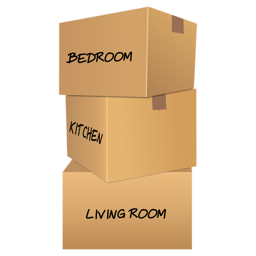
Why do we call it a stack? Think about a stack of boxes. When you stack boxes, you can do one of two things: put boxes onto the stack and take boxes off of the stack. And here is the key. You can only put boxes on the top of the stack, and you can only take boxes off the top of the stack. That’s how stacks work in programming as well!

A stack is what we call a “Last In First Out”, or LIFO, data structure. That means that when we pop a piece of data off the stack, we get the last piece of data we put on the stack.

Stacks in the Real World

So, where do we see stacks in the real world? A great example is repairing an automobile. It is much easier to put a car back together if we put the pieces back on in the reverse order we took them off. Thus, as we take parts off a car, it is highly recommended that we lay them out in a line. Then, when we are ready to put things back together, we can just start at the last piece we took off and work our way back. This operation is exactly how a stack works.

Another example is a stack of chairs. Often in schools or in places that hold different types of events, chairs are stacked in large piles to make moving the chairs easier and to make their storage more efficient. Once again, however, if we are going to put chairs onto the stack or remove chairs from the stack, we are going to have to do it from the top.

Stacks in Code

How do we implement stacks in code? One way would be to use something we already understand, an array. Remember that arrays allow us to store multiple items, where each entry in the array has a unique index number. This is a great way to implement stacks. We can store items directly in the array and use a special top variable to hold the index of the top of the stack.

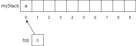
The following figure shows how we might implement a stack with an array. First, we define our array myStack to be an array that can hold 10 numbers, with an index of 0 to 9. Then we create a top variable that keeps track of the index at the top of the array.

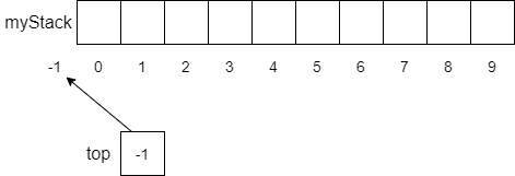
Notice that since we have not put any items onto the stack, we initialize top to be -1. Although this is not a legal index into the array, we can use it to recognize when the stack is empty, and it makes manipulating items in the array much simpler. When we want to push an item onto the stack, we follow a simple procedure as shown below. Of course, since our array has a fixed size, we need to make sure that we don’t try to put an item in a full array. Thus, the precondition is that the array cannot be full. Enforcing this precondition is the function of the if statement at the beginning of the function. If the array is already full, then we’ll throw an exception and let the user handle the situation. Next, we increment the top variable to point to the next available location to store our data. Then it is just a matter of storing the item into the array at the index stored in top.

function PUSH(ITEM)
    if MYSTACK is full then
        throw exception
    end if
    TOP = TOP + 1
    MYSTACK[TOP] = ITEM
end function

If we call the function push(a) and follow the pseudocode above, we will get an array with a stored in myStack[0] and top will have the value 0 as shown below.

As we push items onto the stack, we continue to increment top and store the items on the stack. The figure below shows how the stack would look if we performed the following push operations.

push("b")
push("c")
push("d")
push("e")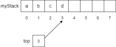

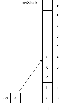
Although we are implementing our stack with an array, we often show stacks vertically instead of horizontally as shown below. In this way the semantics of top makes more sense.

Of course, the next question you might ask is “how do we get items off the stack?”. As discussed above, we have a special operation called pop to take care of that for us. The pseudocode for the pop operation is shown below and is similar in structure to the push operation.

function POP
    if TOP == -1 then
        throw exception
    end if
    TOP = TOP - 1
    return MYSTACK[TOP + 1]
end function

However, instead of checking to see if the stack is full, we need to check if the stack is empty. Thus, our precondition is that the stack is not empty, which we evaluate by checking if top is equal to -1. If it is, we simply throw an exception and let the user handle it. If myStack is not empty, then we can go ahead and perform the pop function. We simply decrement the value of top and return the value stored in myStack[top+1].

Now, if we perform three straight pop operations, we get the following stack.

Stack Operations

The following table shows an example of how to use the above operations to create and manipulate a stack. It assumes the steps are performed sequentially and the result of the operation is shown.

Step	Operation	Effect
1	Constructor	Creates an empty stack.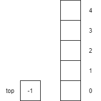
2	isFull()	Returns false since top is not equal to the capacity of the stack.
3	isEmpty()	Returns true since top is equal to -1
4	push(1)	Increments top by 1 and then places item $1$ onto the top of the stack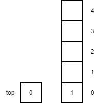
5	push(2)	Increments top by 1 and then places item $2$ onto the top of the stack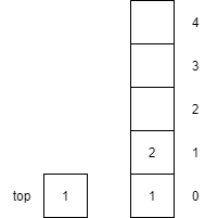
6	push(3)	Increments top by 1 and then places item $3$ onto the top of the stack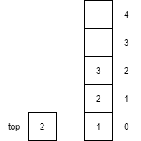
7	peek()	Returns the item $3$ on the top of the stack but does not remove the item from the stack. top is unaffected by peek
8	pop()	Returns the item $3$ from the top of the stack and removes the item from the stack. top is decremented by 1.
9	pop()	Returns the item $2$ from the top of the stack and removes the item from the stack. top is decremented by 1.
10	pop()	Returns the item $1$ from the top of the stack and removes the item from the stack. top is decremented by 1.
11	isEmpty()	Returns true since top is equal to -1

Using a Stack

Stacks are useful in many applications. Classic real-world software that uses stacks includes the undo feature in a text editor, or the forward and back features of web browsers. In a text editor, each user action is pushed onto the stack as it is performed. Then, if the user wants to undo an action, the text editor simply pops the stack to get the last action performed, and then undoes the action. The redo command can be implemented as a second stack. In this case, when actions are popped from the stack in order to undo them, they are pushed onto the redo stack.

Maze Explorer

Another example is a maze exploration application. In this application, we are given a maze, a starting location, and an ending location. Our first goal is to find a path from the start location to the end location. Once we’ve arrived at the end location, our goal becomes returning to the start location in the most direct manner.

We can do this simply with a stack. We will have to search the maze to find the path from the starting location to the ending location. Each time we take a step forward, we push that move onto a stack. If we run into a dead end, we can simply retrace our steps by popping moves off the list and looking for an alternative path. Once we reach the end state, we will have our path stored in the stack. At this point it becomes easy to follow our path backward by popping each move off the top of the stack and performing it. There is no searching involved.

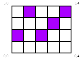
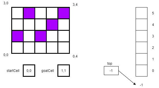
We start with a maze, a startCell, a goalCell, and a stack as shown below. In this case our startCell is 0,0 and our end goal is 1,1. We will store each location on the stack as we move to that location. We will also keep track of the direction we are headed: up, right, down, or left, which we’ll abbreviate as u,r,d,and l.

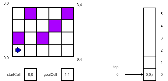
In our first step, we will store our location and direction 0,0,u on the stack.

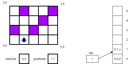
For the second step, we will try to move “up”, or to location 1,0. However, that square in the maze is blocked. So, we change our direction to r as shown below.

After turning right, we attempt to move in that direction to square 0,1, which is successful. Thus, we create a new location 0,1,u and push it on the stack. (Here we always assume we point up when we enter a new square.) The new state of the maze and our stack are shown below.

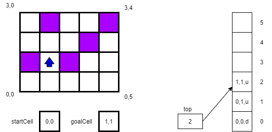
Next, we try to move to 1,1, which again is successful. We again push our new location 1,1,u onto the stack. And, since our current location matches our goalCell location (ignoring the direction indicator) we recognize that we have reached our goal.

Of course, it’s one thing to find our goal cell, but it’s another thing to get back to our starting position. However, we already know the path back given our wise choice of data structures. Since we stored the path in a stack, we can now simply reverse our path and move back to the start cell. All we need to do is pop the top location off of the stack and move to that location over and over again until the stack is empty. The pseudocode for following the path back home is simple.

loop while !MYSTACK.ISEMPTY()
	NEXTLOCATION = MYSTACK.POP()
	MOVETO(NEXTLOCATION)
end while

Path Finding Algorithm

The pseudocode for finding the initial path using the stack is shown below. We assume the enclosing class has already defined a stack called myStack and the datatype called Cell, which represents the squares in the maze. The algorithm also uses three helper functions as described below:

• getNextCell(maze, topCell): computes the next cell based on our current cell’s location and direction;
• incrementDirection(topCell): increments a cell’s direction attribute following the clockwise sequence of up, right, down, left, and then finally done, which means that we’ve tried all directions; and
• valid(nextCell): determines if a cell is valid. A cell is invalid if it is “blocked”, is outside the boundaries of the maze, or is in the current path (i.e., if it exists in the stack).

The parameters of findPath are a 2-dimensional array called maze, the startCell and the endCell. The algorithm begins by pushing the startCell onto myStack. The cell at the top of the stack will always represent our current cell, while the remaining cells in the stack represent the path of cells taken to reach the current cell.

Next, we enter a loop, where we will do the bulk of the work. We peek at the cell on the top of the stack in order to use it in our computations. If the topCell is equal to our goalCell, then we are done and return true indicating that we have found a path to the goal.

If we are not at our goal, we check to see if we have searched all directions from the current cell. If that is the case, then the direction attribute of the topCell will have been set to done. If the direction attribute of topCell is equal to done, then we pop the topCell of the stack, effectively leaving that cell and returning to the next cell in the stack. This is an algorithmic technique called backtracking.

function FINDPATH(MAZE, STARTCELL, GOALCELL)
    MYSTACK.PUSH(STARTCELL);
	loop while !MYSTACK.ISEMPTY()
        TOPCELL = MYSTACK.PEEK()
		if TOPCELL equals GOALCELL
			return true
		if TOPCELL.GETDIRECTION() = done then
            MYSTACK.POP()
		else
            NEXTCELL = GETNEXTCELL(MAZE, TOPCELL)
            INCREMENTDIRECTION(TOPCELL)	
			if VALID(MAZE, NEXTCELL) then
				if MYSTACK.ISFULL() then
                    MYSTACK.DOUBLECAPACITY();
				end if
                MYSTACK.PUSH(NEXTCELL)
			end if 
		end if
	end while 
	return false
end function

However, if we have not searched in all directions from topCell, we will try to explore a new cell (nextCell) adjacent to the topCell. Specifically, nextCell will be the adjacent cell in the direction stored by the direction attribute. We then increment the direction attribute of the topCell so if we end up backtracking, we will know which direction to try next.

Before we push the nextCell onto the stack, we must first check to see if it’s a valid cell by calling the helper function valid. A cell is valid if it is open to be explored. A cell is invalid if it is “blocked,” is outside the boundaries of the maze, or is in the current path (i.e., if it exists in the stack). To help us determine if a cell is in the stack, we will need to extend our stack operations to include a find operation that searches the stack while leaving its contents intact. You will get to implement this operation in your project.

If nextCell is valid, we then check to make sure that the stack is not already full. If it is, we simply call doubleCapacity and continue on our way. Then we push nextCell onto myStack so it will become our next topCell on the next pass through the loop.

After we have explored all possible paths through the maze, the loop will eventually end, and the operation will return false indicating no path was found. While this is not the most efficient path finding algorithm, it is a good example of using stacks for backtracking. Also, if we do find a path and return, the path will be saved in the stack. We can then use the previous pseudocode for retracing our steps and going back to the startCell.

What is a Queue?

A queue (pronounced like the letter “q”) data structure organizes data in a First In, First Out (FIFO) order: the first piece of data put into the queue is the first piece of data available to remove from the queue. A queue functions just like the line you would get into to go into a ballgame, movie, or concert: the person that arrives first is the first to get into the venue.

¹

You might be thinking that this sounds a lot like the stack structure we studied a few modules back, with the exception that the stack was a Last in, First Out (LIFO) structure. If so, you are correct. The real difference between a stack and a queue is how we take data out of the data structure. In a stack, we put data onto the top of the stack and removed it from the top as well. With a queue, we put data onto the end (or rear) of the queue and remove it from the start (or front) of the queue.

Queues in the Real World

The name for queues comes the word in British English used to describe a line of people. Instead of forming lines to wait for some service, British form queues. Thus, when we think of queues, often the first picture to come to mind is a group of people standing in a line. Of course, this is exactly how a computer queue operates as well. The first person in line gets served first. If I get into line before you do, then I will be served before you do.

¹

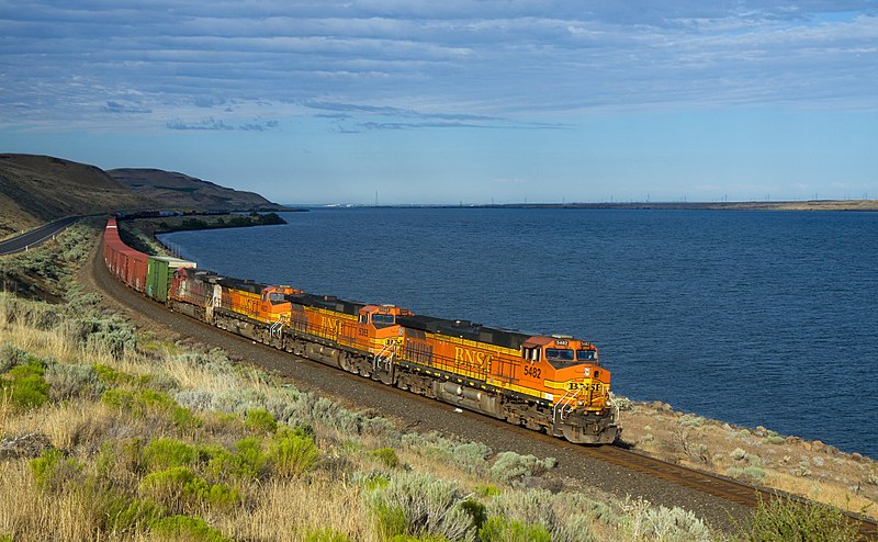
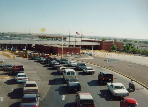
Of course, there are other examples of queues besides lines of people. You can think of a train as a long line of railway cars. They are all connected and move together as the train engine pulls them. A line of cars waiting to go through a toll booth or to cross a border is another good example of a queue. The first car in line will be the first car to get through the toll booth. In the picture below, there are actually several lines.

²

Queues in Code

How do we implement queues in code? Like we did with stacks, we will use an array, which is an easily understandable way to implement queues. We will store data directly in the array and use special start and end variables to keep track of the start of the queue and the end of the queue.

The following figure shows how we might implement a queue with an array. First, we define our array myQueue to be an array that can hold 10 numbers, with an index of 0 to 9. Then we create a start variable to keep track of the index at the start of the queue and an end variable to keep track of the end of the array.

Notice that since we have not put any items into the queue, we initialize start to be -1. Although this is not a legal index into the array, we can use it like we did with stacks to recognize when we have not yet put anything into the queue. As we will see, this also makes manipulating items in the array much simpler. However, to make our use of the array more efficient, -1 will not always indicate that the queue is empty. We will allow the queue to wrap around the array from the start index to the end index. We’ll see an example of this behavior later.

When we want to enqueue an item into the queue, we follow the simple procedure as shown below. Of course, since our array has a fixed size, we need to make sure that we don’t try to put an item in a full array. Thus, the precondition is that the array cannot be full. Enforcing this precondition is the function of the if statement at line 2. If the array is already full, then we’ll throw an exception in line 3 and let the caller handle the situation. Next, we store item at the end location and then compute the new value of end in line 5. Line 6 uses the modulo operator % to return the remainder of the division of $(\text{end} + 1) / \text{length of myQueue}$. In our example, this is helpful when we get to the end of our ten-element array. If end == 9 before enqueue was called, the function would store item in myQueue[9] and then line 4 would cause end to be $(9 +1) % 10$ or $10 % 10$ which is simply $0$, essentially wrapping the queue around the end of the array and continuing it at the beginning of the array.

 1function ENQUEUE (item)
 2  if ISFULL() then
 3    raise exception
 4  end if	
 5  MYQUEUE[END] = ITEM	
 6  END = (END + 1) % length of MYQUEUE
 7  if START == -1
 8    START = 0
 9  end if
10end function

Given our initial configuration above, if we performed an enqueue(7) function call, the result would look like the following.

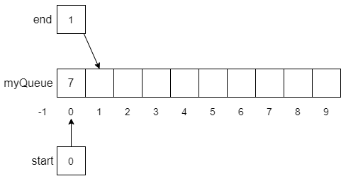
Notice that the value 7 was stored at myQueue[0] in line 5, end was updated to 1 in line 6, and start was set to 0 in line 8. Now, let’s assume we continue to perform enqueue operations until myQueue is almost filled as shown below.

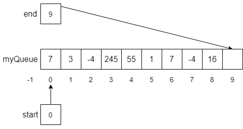
If at this point, we enqueue another number, say -35, the modulo operator in line 6 would help us wrap the end of the list around the array and back to the beginning as expected. The result of this function call is shown below.

Now we have a problem! The array is full of numbers and if we try to enqueue another number, the enqueue function will raise an exception in line 3. However, this example also gives us insight into what the isFull condition should be. Notice that both start, and end are pointing at the same array index. You may want to think about this a little, but you should be able to convince yourself that whenever start == end we will be in a situation like the one above where the array is full, and we cannot safely enqueue another number.

To rectify our situation, we need to have a function to take things out of the queue. We call this function dequeue, which returns the item at the beginning of the queue (pointed at by start) and updates the value of start to point to the next location in the queue. The pseudocode for the dequeue is shown below.

 1function DEQUEUE ()
 2  if ISEMPTY() then
 3    raise exception
 4  end if 
 5  ITEM = MYQUEUE[START]
 6  START = (START + 1) % length of MYQUEUE
 7  if START == END
 8    START = -1
 9    END = 0
10  end if
11  return ITEM
12end function

Line 2 checks if the queue is empty and raises an exception in line 3 if it is. Otherwise, we copy the item at the start location into item at line 5 and then increment the value of start by 1, using the modulo operator to wrap to the beginning of the array if needed in line 6. However, if we dequeue the last item in the queue, we will actually run into the same situation that we ran into in the enqueue when we filled the array, start == end. Since we need to differentiate between being full or empty (it’s kind of important!), we reset the start and end values back to their initial state when we dequeue the last item in the queue. That is, we set start = -1 and end = 0. This way, we will always be able to tell the difference between the queue being empty or full. Finally, we return the item to the calling function in line 11.

Using Operations

The following table shows an example of how to use the above operations to create and manipulate a queue. It assumes the steps are performed sequentially and the result of the operation is shown.

Step	Operation	Effect
1	Constructor	Creates an empty queue of capacity 3.
2	isFull()	Returns false since start is not equal to end
3	isEmpty()	Returns true since start is equal to -1.
4	enqueue(1)	Places item 1 onto queue at the end and increments end by 1.
5	enqueue(2)	Places item 2 onto queue at the end and increments end by 1.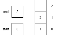
6	enqueue(3)	Places item 3 onto queue at the end and sets end to end+1 modulo the size of the array (3). The result of the operation is 0, thus end is set to 0.
7	peek()	Returns the item 1 on the start of the queue but does not remove the item from the queue. start and end are unaffected by peek.
8	isFull()	Returns true since start is equal to end
9	dequeue()	Returns the item 1 from the start of the queue. start is incremented by 1, effectively removing 1 from the queue.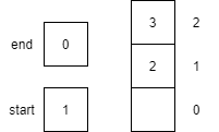
10	dequeue()	Returns the item 2 from the start of the queue. start is incremented by 1, effectively removing 2 from the queue.
11	enqueue(4)	Places item 4 onto queue at the end and increments end.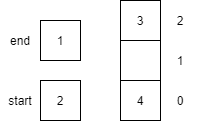
12	dequeue()	Returns the item 3 from the start of the queue. start is set to start+1 modulo the size of the array (3). The result of the operation is 0, thus start is set to 0.
13	dequeue()	Returns the item 4 from the start of the queue. start is incremented by 1, and since start == end, they are both reset to -1 and 0 respectively.
14	isEmpty()	Returns true since start is equal to -1.

Using a Queue

Queues are useful in many applications. Classic real-world software which uses queues includes the scheduling of tasks, sharing of resources, and processing of messages in the proper order. A common need is to schedule tasks to be executed based on their priority. This type of scheduling can be done in a computer or on an assembly line floor, but the basic concept is the same.

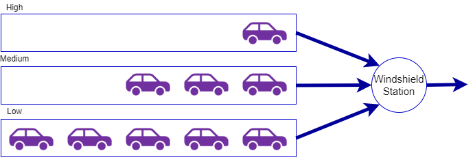
Let’s assume that we are putting windshields onto new cars in a production line. In addition, there are some cars that we want to rush through production faster than others. There are actually three different priorities:

1. High priority: these cars have been ordered by customers who are waiting for them.
2. Medium priority: these cars have been ordered as “fleet cars” for specific companies.
3. Low priority: these cars are cars used to fill dealer inventories.

Ideally, as cars come to the windshield station, we would be able to put their windshields in and send them to the next station before we received the next car. However, this is rarely the case. Since putting on windshields often requires special attention, cars tend to line up to get their windows installed. This is when their priority comes into account. Instead of using a simple queue to line cars up first-come, first-served in FIFO order, we would like to jump high priority cars to the head of the line.

While we could build a sophisticated queueing mechanism that would automatically insert cars in the appropriate order based on priority and then arrival time, we could also use a queue to handle each set of car priorities. A figure illustrating this situation is shown below. As cars come in, they are put in one of three queues: high priority, medium priority, or low priority. When the windshield station completes a car it then takes the next car from the highest priority queue.

The interesting part of the problem is the controller at the windshield station that determines which car will be selected to be worked on next. The controller will need to have the following interface:

function receiveCar(car, priority)
 // receives a car from the previous station and places into a specific queue

function bool isEmpty()
 // returns true if there are no more cars in the queue

function getCar() returns car
 // retrieves the next car based on priority

Using this simple interface, we will define a class to act as the windshield station controller. It will receive cars from the previous station and get cars for the windshield station.

We start by defining the internal attributes and constructor for the Controller class as follows, using the Queue functions defined earlier in this module. We first declare three separate queues, one each for high, medium, and low priority cars. Next, we create the constructor for the Controller class. The constructor simply initializes our three queues with varying capacities based on the expected usage of each of the queues. Notice, that the high priority queue has the smallest capacity while the low priority queue has the largest capacity.

class Controller
    declare HIGH as a Queue
    declare MEDIUM as a Queue
    declare LOW as a Queue

    function Controller()
        HIGH = new Queue(4)
        MEDIUM = new Queue(6)
        LOW = new Queue(8)
    end function

Next, we need to define the interface function as defined above. We start with the receiveCar function. There are three cases based on the priority of the car. If we look at the first case for priority == high, we check to see if the high queue is full before calling the enqueue function to place the car into the high queue. If the queue is full, we raise an exception. We follow the exact same logic for the medium and low priority cars as well. Finally, there is a final else that captures the case where the user did not specific either high, medium, or low priority. In this case, an exception is raised.

function receiveCar(CAR, PRIORITY)
    if PRIORITY == high
        if HIGH.isFull()
            raise exception
        else
            HIGH.enqueue(CAR)
        end if
    else PRIORITY == medium
        if MEDIUM.isFull()
            raise exception
        else
            MEDIUM.enqueue(CAR)
        end if
    else PRIORITY == low
        if LOW.isFull()
            raise exception
        else
            LOW.enqueue(CAR)
        end if
    else
        raise exception
    end if
end function

Now we will define the isEmpty function. While we do not include an isFull function due to the ambiguity of what that would mean and how it might be useful, the isEmpty function will be useful for the windshield station to check before they request another call via the getCar function.

As you can see below, the isEmpty function simply returns the logical AND of each of the individual queue’s isEmpty status. Thus, the function will return true if, and only if, each of the high, medium, and low queues are empty.

function isEmpty()
    return HIGH.isEmpty() and MEDIUM.isEmpty() and LOW.isEmpty()
end function

Finally, we are able to define the getCar function. It is similar in structure to the receiveCar function in that it checks each queue individually. In the case of getCar, the key to the priority mechanism we are developing is in the order we check the queues. In this case, we check them in the expected order from high to low. If the high queue is not empty, we get the car from that queue and return it to the calling function. If the high queue is empty, then we check the medium queue. Likewise, if the medium queue is empty, we check the low queue. Finally, if all of the queues are empty, we raise an exception.

function getCar()
    if not HIGH.isEmpty()
        return HIGH.dequeue()
    else not MEDIUM.isEmpty()
        return MEDIUM.dequeue()
    else not LOW.isEmpty()
        return LOW.dequeue()
    else
        raise exception
    end if
end function

Windshield Station Example

The following example shows how the Controller class would work, given specific calls to receiveCar and getCar.

Step	Operation	Effect
1	Constructor	Creates 3 priority queues.
2	getCar()	Raises an exception since all three queues will be empty.
3	receiveCar(a, low)	Places car a into the low queue.
4	receiveCar(b, low)	Places car b into the low queue.
5	receiveCar(f, high)	Places car f into the high queue.
6	receiveCar(d, medium)	Places car d into the medium queue.
7	receiveCar(g, high)	Raises an exception since the high queue is already full.
8	receiveCar(e, medium)	Places car e into the medium queue.
9	getCar()	Returns car f from the high queue.
10	getCar()	Returns car d from the medium queue.
11	getCar()	Returns car e from the medium queue.
12	getCar()	Returns car a from the low queue.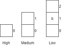
13	getCar()	Returns car b from the low queue.
14	getCar()	Raises an exception since there are no more cars available in any of the three queues.
15	isEmpty()	Returns true since all three queues are empty.

What is a List?

A list is a data structure that holds a sequence of data, such as the shopping list shown below. Each list has a head item and a tail item, with all other items placed linearly between the head and the tail. As we pick up items in the store, we will remove them, or cross them off the list. Likewise, if we get a text from our housemate to get some cookies, we can add them to the list as well.

¹

Lists are actually very general structures that we can use for a variety of purposes. One common example is the history section of a web browser. The web browser actually creates a list of past web pages we have visited, and each time we visit a new web page it is added to the list. That way, when we check our history, we can see all the web pages we have visited recently in the order we visited them. The list also allows us to scroll through the list and select one to revisit or select another one to remove from the history altogether.

Of course, we have already seen several instances of lists so far in programming, including arrays, stacks, and queues. However, lists are much more flexible than the arrays, stacks, and queues we have studied so far. Lists allow us to add or remove items from the head, tail, or anywhere in between. We will see how we can actually implement stacks and queues using lists later in this module.

Lists in the Real World

Most of us see and use lists every day. We have a list for shopping as we saw above, but we may also have a “to do” list, a list of homework assignments, or a list of movies we want to watch. Some of us are list-makers and some are not, but we all know a list when we see it.

¹

However, there are other lists in the real world that we might not even think of as a list. For instance, a playlist on our favorite music app is an example of a list. A music app lets us move forward or backward in a list or choose a song randomly from a list. We can even reorder our list whenever we want.

All the examples we’ve seen for stacks and queues can be thought of as lists as well. Stacks of chairs or moving boxes, railroad trains, and cars going through a tollbooth are all examples of special types of lists.

Lists in Code

The Problem With Arrays

To this point, we have been using arrays as our underlying data structures for implementing linear data structures such as stacks and queues. Given that with stacks and queues we only put items into the array and remove from either the start or end of the data structure, we have been able to make arrays work. However, there are some drawbacks to using arrays for stacks and queues as well as for more general data structures.

1. We can run out of room in our array for our stacks or queues.
2. There is no good way to use memory efficiently. We have to use expensive “double” and “halve” capacity operations for stacks and queues when we need to use more or less memory.
3. Inserting an item into the middle of a sorted list will be very costly in memory. In an array, we will have to move several items to keep the list in order.

While drawbacks 1 and 2 above can be overcome (albeit rather awkwardly) when using arrays for stacks and queues, drawback 3 becomes a real problem when trying to use more general list structures. If we insert an item into the middle of an array, we must move several other items “down” the array to make room.

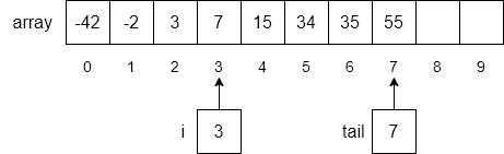
If for example, if we want to insert the number 5 into the sorted array shown below, we have to carry out several steps:

1. Find the index of the first item whose value is greater than the number we want to insert into the array. We will call this index i,
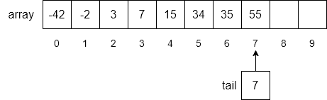
2. Shift each item from index i to the end of the list down one place location in the array,
3. Insert the new item into the array at index i, and
4. Update the index to the tail of the list.

In our example, step 1 will loop through each item of the array until we find the first number in the array greater than 5. As shown below, the number 7 is found in index 3.

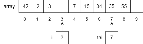
Next, we will use another loop to move each item from index i to the end of the array down by one index number as shown below.

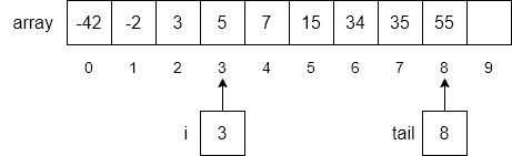
Finally, we will insert our new number, 5, into the array at index 3 and increment tail to 8.

In this operation, if we have $N$ items, we either compare or move all of them, which would require $N$ operations. Of course, this operation runs in order $N$ time.

The same problem occurs when we remove an item from the array. In this case we must perform the following steps:

1. Search the array to find the first occurrence of the desired number to remove,
2. Continue searching until we find the last occurrence of the desired number to remove,
3. Shift each item after the last occurrence of our desired number “up” the array, once for each desired number being removed from the array, and
4. Update the index to the tail of the list.

A More Flexible Approach

Instead of using arrays to try to hold our lists, a more flexible approach is to build our own list data structure that relies on a set of objects that are all linked together through references to each other. In the figure below we have created a list of numbers that are linked to each other. Each object contains both the number as well as a reference to the next number in the list. Using this structure, we can search through each item in the list by starting sequentially from the beginning and performing a linear search much like we did with arrays. However, instead of explicitly keeping track of the end of the list, we use the convention that the reference in the last item of the list is set to 0, which we call null. If a reference is set to null we interpret this to mean that there is no next item in the list. This “linked list” structure also makes inserting items into the middle of the list easier. All we need to do is find the location in the list where we want to insert the item and then adjust the references to include the new item into the list.

The following figure shows a slightly more complex version of a linked list, called a “doubly linked list”. Instead of just having each item in the list reference the next item, it references the previous item in the list as well. The main advantage of doubly linked lists is that we can easily traverse the list in either the forward or backward direction. Doubly linked lists are useful in applications to implement undo and redo functions, and in web browser histories where we want the ability to go forward and backward in the history.

We will investigate each of these approaches in more detail below and will reimplement both our stack and queue operations using linked lists instead of arrays.

Doubly Linked Lists

With singly linked lists, each node in the list had a pointer to the next node in the list. This structure allowed us to grow and shrink the list as needed and gave us the ability to insert and delete nodes at the front, middle, or end of the list. However, we often had to use two pointers when manipulating the list to allow us to access the previous node in the list as well as the current node. One way to solve this problem and make our list even more flexible is to allow a node to point at both the previous node in the list as well as the next node in the list. We call this a doubly linked list.

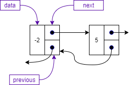
The concept of a doubly linked list is shown below. Here, each node in the list has a link to the next node and a link to the previous node. If there is no previous or next node, we set the pointers to null.

Doubly Linked Node

A doubly linked list node is the same as a singly linked list node with the addition of the previous attribute that points to the previous node in the list as shown below.

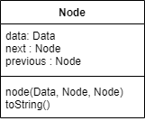
The class representation of a doubly linked list Node is shown below. As discussed above, we have three attributes:

• data, which holds the data of the node,
• next, which is a pointer to the next node, and
• previous, which is a pointer to the previous node.

We also use a constructor and the standard toString operation to create a string for the data stored in the node.

Doubly Linked List

As with our singly linked list, we start off a doubly linked list with a pointer to the first node in the list, which we call head. However, if we also store the pointer to the last node in the list, we can simplify some of our insertion and removal operations as well as reduce the time complexity of operations that insert, remove, or peek at the last node in the list.

The figure below shows a doubly linked list with five nodes. The variable head points to the first node in the list, while the variable tail points to the last node in the list. Each node in the list now has two pointers, next and previous, which point to the appropriate node in the list. Notice that the first node’s previous pointer is null, while the last node’s next pointer is also null.

Doubly Linked List Class

Like we did for our singly linked list, we capture the necessary details for our doubly linked list in a class. The doubly linked list class has four attributes:

• head—the pointer to the first node in the list,
• tail—the pointer to the last node in the list,
• current—the pointer to the current node used by the iterator, and
• size—an integer to keep track of the number of items in the list.

Class DoubleLinkedList 
    Node head
    Node tail
    Node current
    Integer size = 0

List Iterators

An iterator is a set of operations a data structure provides to allow users to access the items in the data structure sequentially, without requiring them to know its underlying representation. There are many reasons users might want to access the data in a list. For instance, users may want to make a copy of their list or count the number of times a piece of data was stored in the list. Or, the user might want to delete all data from a list that matches a certain specification. All of these can be handled by the user using an iterator.

At a minimum, iterators have two operations: reset and getNext. Both of these operations use the list class’s current attribute to keep track of the iterator’s current node.

Reset

The reset operation initializes or reinitializes the current pointer. It is typically used to ensure that the iterator starts at the beginning of the list. All that is required is for the current attribute be set to null.

function reset()
  current = null
end function

Get Next

The main operation of the iterator is the getNext operation. Basically, the getNext operation returns the next available node in the list if one is available. It returns null if the list is empty or if current is pointing at the last node in the list.

Lines 2 and 3 in the getNext operation check to see if we have an empty list, which results in returning the null value. If we have something in the list but current is null, this indicates that the reset operation has just been executed and we should return the data in the first node. Therefore, we set current = head in line 6. Otherwise, we set the current pointer to point to the next node in the list in line 8.

 1function getNext() returns data
 2  if isEmpty()
 3    return null
 4  end if 
 5  if current == null
 6    current = head
 7  else
 8    current = current.next
 9  end if
10  if current == null
11    return null
12  else
13    return current.data
14  end if
15end function

Next we return the appropriate data. If current == null we are at the end of the list and so we return the null value in line 11. If current is not equal to null, then it is pointing at a node in the list, so we simply return current.data in line 13.

Remove current

While not technically part of the basic iterator interface, the removeCurrent operation is an example of operations that can be provided to work hand-in-hand with a list iterator. The removeCurrent operation allows the user to utilize the iterator operations to find a specific piece of data in the list and then remove that data from the list. Other operations that might be provided include being able to replace the data in the current node, or even insert a new piece of data before or after the current node.

The removeCurrent operation starts by checking to make sure that current is really pointing at a node. If it is not, then the condition is caught in line 2 and an exception is raised in line 3. Next, we set the next pointer in the previous node to point to the current node’s next pointer in lines 5 - 9, taking into account whether the current node is the first node in the list. After that, we set the next node’s previous pointer to point back at the previous node in line 10 - 14, considering whether the node is the last node in the list. Finally, we decrement size in line 15.

function removeCurrent()
  if current == null
    raise exception
  end if
  if current.previous != null
    current.previous.next = current.next
  else
    head = current.next
  end
  if current.next != null
    current.next.previous = current.previous
  else
    tail = current.previous
  end if
    current = current.previous
  size – size – 1
end function

Using an Iterator

There are several applications for list iterators. For our example, we will use the case where we need a function to delete all instances of data in the list that match a given piece of data. Our deleteAll function resides outside the list class, so we will have to pass in the list we want to delete the data from. We start the operation by initializing the list iterator in line 2, followed by getting the first piece of data in the list in line 3. Next, we’ll enter a while loop and stay in that loop as long as our copy of the current node in the list, listData, is not null. When it becomes null, we are at the end of the list and we can exit the loop and the function.

function deleteAll(list, data)
  list.reset()
  listData = list.getNext()
  while listData != null
    if listData == data
      list.removeCurrent()
    end if	
    listData = list.getNext()
  end while
end function

Once in the list, it’s a matter of checking if our listData is equal to the data we are trying to match. If it is, we call the list’s removeCurrent operation. Then, at the bottom of the list, we get the next piece of data from the list using the list iterator’s getNext operation.

By using a list iterator and a limited set of operations on the current data in the list, we can allow list users to manipulate the list while ensuring that the integrity of the list remains intact. Since we do not know ahead of time how a list will be used in a given application, an iterator with associated operations can allow the user to use the list in application-specific ways without having to add new operations to the list data structure.

List-Based Queues

Implementing a queue with a doubly linked list is straightforward and efficient. The core queue operations (enqueue, dequeue, isEmpty, and peek) can all be implemented by directly calling list operations that run in constant time. The only other major operation is the toString operation, which is also implemented by directly calling the list toString operation; however, it runs in order $N$ time due to the fact that the list toString operation must iterate through each item in the list.

The key queue operations and their list-based implementations are shown below.

function enqueue (data)
    list.append(data)
end function

function dequeue() returns data
    return removeFirst()
end function

function isEmpty() returns Boolean
    return list.isEmpty()
end function

function peek() returns data
    return list.peek()
end function

function toString() returns data
    return list.toString()
end function

Stacks can be implemented using a similar method - namely adding and removing from the end of the list. This can even be done using a singly-linked list, and is very efficient.

Lists Summary

In this module we looked at the stack data structure. Stacks are a “last in first out” data structure that use two main operations, push and pop, to put data onto the stack and to remove data off of the stack. Stacks are useful in many applications including text editor “undo” and web browser “back” functions.

We also saw the queue data structure. Queues are a “first in first out” data structure that use two main operations, enqueue and dequeue, to put data into the queue and to remove data from the queue. Queues are useful in many applications including the scheduling of tasks, sharing of resources, and processing of messages in the proper order.

Finally, we introduced the concept of a linked list, discussing both singly and doubly linked lists. Both kinds of lists are made up of nodes that hold data as well as references (also known as pointers) to other nodes in the list. Singly linked lists use only a single pointer, next, to connect each node to the next node in the list. While simple, we saw that a singly linked list allowed us to efficiently implement a stack without any artificial bounds on the number of items in the list.

With doubly linked lists, we added a previous pointer that points to the previous node. This makes the list more flexible and makes it easier to insert and remove nodes from the list. We also added a tail pointer to the class, which keeps track of the last node in the list. The tail pointer significantly increased the efficiency of working with nodes at the end of the list. Adding the tail pointer allowed us to implement all the major queue operations in constant time.