Chapter 8
Performance & String Builder
Choosing the correct data structures & writing efficient programs that use strings!
Choosing the correct data structures & writing efficient programs that use strings!
There are several linear data structures that we can use in our programs, including stacks, queues, lists, sets, and hash tables. In this course, we have covered each of these structures in detail. However, as a programmer, one of the most difficult decisions we will make when developing a program is the choice of which data structure to use. Sometimes the choice may be obvious based on the data we plan to store or the algorithms we need to perform, but in practice that happens very rarely. Instead, we are faced with competing tradeoffs between various factors such as ease of use, performance, and simplicity.
In this chapter, we’ll review the various data structures and algorithms we’ve learned about in this course, but this time we’ll add a bit more focus on the decisions a programmer would make when choosing to use a particular data structure or algorithm.
The choice of which data structure to use is often the most consequential choice we make when developing a new piece of software, as it can have a large impact on the overall performance of the program. While there are many different factors to consider, here are three important questions we can ask when choosing a data structure:
By answering the questions above in the order they are presented, we should be able to make good decisions about which data structures would work best in our program. We are purposely putting more focus on writing working and understandable code instead of worrying about performance. This is because many programs are only used with small data sets on powerful modern computers, so performance is not the most important aspect. However, there are instances where performance becomes much more important, and in those cases more focus can be placed on finding the most performant solution as well.
As it turns out, these three questions are very similar to a classic (trilemma)[https://en.wikipedia.org/wiki/Trilemma] from the world of business, as shown in the diagram below.
In the world of software engineering, it is said that the process of developing a new program can only have two of the three factors of “good”, “fast”, and “cheap”. The three questions above form a similar trilemma. Put another way, there will always be competing tradeoffs when selecting a data structure for our programs.
For example, the most performant option may not be as easy to understand, and it may be more difficult to debug and ensure that it works correctly. A great example of this is matrix multiplication, a very common operation in the world of high-performance computing. A simple solution requires just three loops and is very easy to understand. However, the most performant solution requires hundreds of lines of code, assembly instructions, and a deep understanding of the hardware on which the program will be executed. That program will be fast and efficient, but it is much more difficult to understand and debug.
File:Project-triangle.svg. (2020, January 12). Wikimedia Commons, the free media repository. Retrieved 21:09, April 30, 2020 from https://commons.wikimedia.org/w/index.php?title=File:Project-triangle.svg&oldid=386979544. ↩︎
Data structures that are used in our programs can be characterized in terms of two performance attributes: processing time and memory usage.
We will not worry about memory usage at this point, since most of the memory used in these data structures is consumed by the data that we are storing. More technically, we would say that the memory use of a data structure containing N elements is on the order of $N$ size. However, some structures, such as doubly linked lists, must maintain both the next and previous pointers along with each element, so there can be a significant amount of memory overhead. That is something we should keep in mind, but only in cases where we are dealing with a large amount of data and are worried about memory usage.
When evaluating the processing time of a data structure, we are most concerned with the algorithms used to add, remove, access, and find elements in the data structure itself. There are a couple of ways we can evaluate these operations.
Throughout this course, we have included mathematical descriptions of the processing time of most major operations on the data structures we have covered.
One of the best ways to compare data structures is to look at the common operations that they can perform. For this analysis, we’ve chosen to analyze the following four operations:
The following table compares the best- and worst-case processing time for many common data structures and operations, expressed in terms of $N$, the number of elements in the structure.
| Data Structure | Insert Best | Insert Worst | Access Best | Access Worst | Find Best | Find Worst | Delete Best | Delete Worst |
|---|---|---|---|---|---|---|---|---|
| Unsorted Array | $1$ | $1$ | $1$ | $1$ | $N$ | $N$ | $N$ | $N$ |
| Sorted Array | $\text{lg}(N)$ | $N$ | $1$ | $1$ | $\text{lg}(N)$ | $\text{lg}(N)$ | $\text{lg}(N)$ | $N$ |
| Array Stack (LIFO) | $1$ | $1$ | $1$ | $1$ | $N$ | $N$ | $1$ | $1$ |
| Array Queue (FIFO) | $1$ | $1$ | $1$ | $1$ | $N$ | $N$ | $1$ | $1$ |
| Unsorted Linked List | $1$ | $1$ | $N$ | $N$ | $N$ | $N$ | $N$ | $N$ |
| Sorted Linked List | $N$ | $N$ | $N$ | $N$ | $N$ | $N$ | $N$ | $N$ |
| Linked List Stack (LIFO) | $1$ | $1$ | $1$ | $1$ | $N$ | $N$ | $1$ | $1$ |
| Linked List Queue (FIFO) | $1$ | $1$ | $1$ | $1$ | $N$ | $N$ | $1$ | $1$ |
| Hash Table | $1$ | $N$ | $1$ | $N$ | $N$ | $N$ | $1$ | $N$ |
We can also compare these processing times by graphing the equations used to describe them. The graph below shows several of the common orders that we have seen so far.
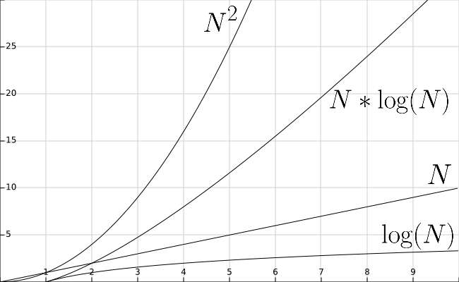
On the next few pages, we will discuss each data structure in brief, using this table to compare the performance of the various data structures we’ve covered in this course.

The next data structure we learned about is the linked list. Specifically, we will look at the doubly linked list in this example, but in most instances the performance of a singly linked list is comparable.
With a linked list, the process of inserting an element at either the beginning or the end is a constant time operation since we maintain both a head and a tail reference. All we must do is create a new node and update a few references and we are good to go.
However, if we would like to access a specific element somewhere in the list, we will have to iterate through the list starting from either the head or the tail until we find the element we need. So, that operation runs in order $N$ time. This is the major difference between linked lists and arrays: with an array, we can directly access items using the array index, but with linked lists we must iterate to get to that element. This becomes important in the next section when we discuss the performance of a sorted linked list.
Similarly, the process of finding an element also requires iterating through the list, which is an operation that runs in order $N$ time.
Finally, if we want to find and delete an element, that also runs in order $N$ time since we must search through the list to find the element. Once we have found the element, the process of deleting that element is a constant time operation. So, if we use our list iterator methods in an efficient manner, the actual run time may be more efficient than this analysis would lead us to believe.

We have not directly analyzed the performance of a sorted linked list in this course, but hopefully the analysis makes sense based on what we have learned before. Since the process of iterating through a linked list runs in order of $N$ time, every operation required to build a sorted linked list is limited by that fact.
For example, if we want to insert an element into a list in sorted order, we must simply iterate through the list to find the correct location to insert it. Once we’ve found it, the process of inserting is actually a constant time operation since we don’t have to shift any elements around, but because we can’t use binary search on a linked list, we don’t have any way to take advantage of the fact that the list is sorted.
The same problem occurs when we want to search for a particular element. Since we cannot use binary search to jump around between various elements in the list, we are limited to a simple linear search process, which runs in order of $N$ time.
Likewise, when we want to search and delete an element from the list, we must once again iterate through the entire list, resulting in an operation that runs in order $N$ time.
So, is there any benefit to sorting a linked list? Based on this analysis, not really! The purpose of sorting a collection is simply to make searching for a particular element faster. However, since we cannot use array indices to jump around a list like we can with an array, we do not see much of an improvement.
However, in the real world, we can improve some of these linear algorithms by “short-circuiting” them. When we “short-circuit” an algorithm, we provide additional code that allows the algorithm to return early if it realizes that it will not succeed.
For example, if we are searching for a particular element in a sorted list, we can add an if statement to check and see if the current element is greater than the element we are searching for. If the list is sorted in ascending order, we know that we have gone past the location where we expected to find our element, so we can just return without checking the rest of the list. While this does not change the mathematical analysis of the running time of this operation, it may improve the real-world empirical analysis of the operation.
We already saw how to use the operations from a linked list to implement both a stack and a queue. Since those data structures restrict the operations we can perform a bit, it turns out that we can use a linked list to implement a stack and a queue with comparable performance to an array implementation.
For example, inserting, accessing, and removing elements in a stack or a queue based on a doubly linked list are all constant time operations, since we can use the head and tail references in a doubly linked list to avoid the need to iterate through the entire list to perform those operations. In fact, the only time we would have to iterate through the entire list is when we want to find a particular element in the stack or the queue. However, since we cannot sort a stack or a queue, finding an element runs in order $N$ time, which is comparable to an array implementation.
By limiting the actions we want to perform with our linked list, we can get a level of performance similar to an array implementation of a stack or a queue. It is a useful outcome that demonstrates the ability of different data structures to achieve similar outcomes.

Analyzing the performance of a hash table is a bit trickier than the other data structures, mainly due to how a hash table tries to use its complex structure to get a “best of both worlds” performance outcome.
For example, consider the insert operation. In the best case, the hash table has a capacity that is large enough to guarantee that there are not any hash collisions. Each entry in the array of the hash table will be an empty list and inserting an element into an empty list is done in constant time, so the whole operation runs in the order of constant time.
The worst case for inserting an item into a hash table would be when every element has the same hash, so every element in the hash table is contained in the same list. In that case, we must iterate through the entire list to make sure the key has not already been used, which would be in the order of $N$ time.
Thankfully, if we properly design our hash table such that the capacity is much larger than our expected size, and the hash function we use to hash our keys results in a properly distributed hash, this worst case scenario should happen very rarely, if ever. Therefore, our expected performance should be closer to constant time.
One important thing to remember, however, is that each operation in a hash table requires computing the hash of the key given as input. Therefore, while some operations may run in constant time, if the action of computing the hash is costly, the overall operation may run very slowly.
The analysis of the operation to access a single element in a hash table based on a given key is similar. If the hash table elements are distributed across the table, then each list should only contain a single element. In that case, we can just compute the hash of the key and determine if that key has been used in a single operation, which runs in the order of constant time.
In the worst case, however, we once again have the situation where all the elements have been placed in the same linked list. We would need to iterate through each element to find the one we are looking for. In that case, the operation would run in the order of $N$ time.
The operation for finding a specific element in a hash table is a bit unique. In this case, we are discussing looking for a particular value, not necessarily a particular key. That operation is discussed in the previous paragraph. For the operation, the only possible way forward is to iterate through each list in the hash table and perform a linear search for the requested value, which will always run in order $N$ time.
Finally, if we want to delete a single element from a hash table based on a given key, the analysis is the same as inserting or finding an element. In the best case, it runs in the order of constant time, but the worst case runs in the order of N time since we must iterate through an entire list of $N$ elements.
Even though a hash table has some very poor performance in the worst case, as discussed earlier those worst case situations are very rare, and as long as we are careful about how we manage the capacity of our hash table and how we compute the hash of our objects, we can expect to see operations running in near constant time during normal usage.
We can examine the performance of the algorithms we use in a similar manner. Once again, we are concerned with both the memory usage and processing time of the algorithm. In this case, we are concerned with the amount of memory required to perform the algorithm that is above and beyond the memory used to store the data in the first place.
When analyzing searching and sorting algorithms, we’ll assume that we are using arrays as our data structure, since they give us the best performance for accessing and swapping random elements quickly.
There are two basic searching algorithms: linear search and binary search.
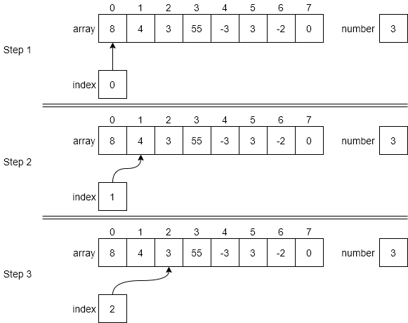
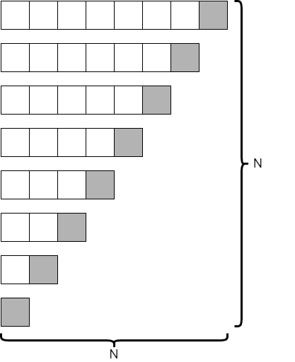
For linear search, we are simply iterating through the entire data structure until we find the desired item. So, while we can stop looking as soon as it is found, in the worst case we will have to look at all the elements in the structure, meaning the algorithm runs in order $N$ time.
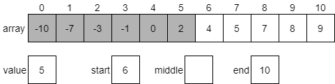
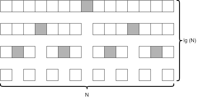
Binary search, on the other hand, takes advantage of a sorted array to jump around quickly. In effect, each element we analyze allows us to eliminate half of the remaining elements in our search. With as few as 8 steps, we can search through an array that contains 64 elements. When we analyze this algorithm, we find that it runs in order $\text{lg}(N)$ time, which is a vast improvement over binary search.
Of course, this only works when we can directly access elements in the middle of our data structure. So, while a linked list gives us several performance improvements over an array, we cannot use binary search effectively on a linked list.
In terms of memory usage, since both linear search and binary search just rely on the original data structures for storing the data, the extra memory usage is constant and consists of just a couple of extra variables, regardless of how many elements are in the data structure.
We have already discussed how much of an improvement binary search is over a linear search. In fact, our analysis showed that performing as few as 7 or 8 linear searches will take more time than sorting the array and using binary search. Therefore, in many cases we may want to sort our data. There are several different algorithms we can use to sort our data, but in this course we explored four of them: selection sort, bubble sort, merge sort, and quicksort.
The selection sort algorithm involves finding the smallest or largest value in an array, then moving that value to the appropriate end, and repeating the process until the entire array is sorted. Each time we iterate through the array, we look at every remaining element. In the module on sorting, we showed (through some clever mathematical analysis) that this algorithm runs in the order of $N^2$ time.
Bubble sort is similar, but instead of finding the smallest or largest element in each iteration, it focuses on just swapping elements that are out of order, and eventually (through repeated iterations) sorting the entire array. While doing so, the largest or smallest elements appear to “bubble” to the appropriate end of the array, which gives the algorithm its name. Once again, because the bubble sort algorithm repeatedly iterates through the entire data structure, it also runs on the order of $N^2$ time.
Both selection sort and bubble sort are inefficient as sorting algorithms go, yet their main value is their simplicity. They are also very nice in that they do not require any additional memory usage to run. They are easy to implement and understand and make a good academic example when learning about algorithms. While they are not used often in practice, later in this module we will discuss a couple of situations where we may consider them useful.
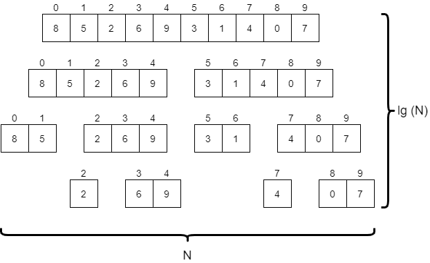
Merge sort is a very powerful divide and conquer algorithm, which splits the array to be sorted into progressively smaller parts until each one contains just one or two elements. Then, once those smaller parts are sorted, it slowly merges them back together until the entire array is sorted. We must look at each element in the array at least once per “level” of the algorithm in the diagram above, so overall this algorithm runs in the order of $N * \text{lg}(N)$ time. This is quite a bit faster than selection sort and bubble sort. However, most implementations of merge sort require at least a second array for storing data as it is merged together, so the additional memory usage is also on the order of $N$.
Quicksort is a very clever algorithm, which involves selecting a “pivot” element from the data, and then dividing the data into two halves, one containing all elements less than the pivot, and another with all items greater than the pivot. Then, the process repeats on each half until the entire structure is sorted. In the ideal scenario, shown in the diagram above, quicksort runs on the order of $N * \text{lg}(N)$ time, similar to merge sort. However, this depends on the choice of the pivot element being close to the median element of the structure, which we cannot always guarantee. Thankfully, in practice, we can just choose a random element (such as the last element in the structure) and we’ll see performance that is close to the $N * \text{lg}(N)$ target.
However, if we choose our pivot element poorly, the worst case scenario shown in the diagram above can occur, causing the run time to be on the order of $N^2$ instead. This means that quicksort has a troublesome, but rare, worst case performance scenario.
There are many different algorithms we can use to sort our data, and some of them can be shown mathematically to be more efficient, even in the worst case. So, how should we choose which algorithm to use?
In practice, it really comes down to a variety of factors, based on the amount of data we expect our program to handle, the randomness of the data, and more. The only way to truly know which algorithm is the best is to empirically test all of them and choose the fastest one, but even that approach relies on us predicting the data that our program will be utilizing.
Instead, here are some general guidelines we can use to help us select a sorting algorithm to use in our program.
Of course, the choice of which sorting algorithm to use is one of the most important decisions a programmer can make, and it is a great example of the fact that there are multiple ways to write a program that performs a particular task. Each possible program comes with various performance and memory considerations, and in many cases, there may not be a correct option. Instead, we must rely on our own knowledge and insight to choose the method that we feel would work best in any given situation.
Throughout this course, we have looked at a few ways we can use the data structures we have already learned to do something useful. In this module, we will look at a few of those examples again, as well as a few more interesting uses of the data structures that we have built.
First and foremost, it is important to understand that we can implement many of the simpler data structures such as stacks, queues and sets using both arrays and linked lists. In fact, from a certain point of view, there are only two commonly used containers for data – the array and the linked list. Nearly all other data structures are a variant of one of those two approaches or a combination of both.
Earlier in this chapter, we discussed some of the performance implications that arise when using arrays or linked lists to implement stacks and queues. In practice, we need to understand how we will be using our data in order to choose between the two approaches.
One unique use of sets appears in the code of compilers and interpreters. In each case, a programming language can only have one instance of a variable with a given name at any one time. So, we can think of the variables in a program as a set. In the code for a compiler or interpreter, we might find many instances of sets that are used to enforce rules that require each variable or function name to be unique.
Of course, this same property becomes important in even larger data storage structures, such as a relational database. For example, a database may include a column for a username or identification number which must be unique, such that no two entries can be the same. Once again, we can use a set to help enforce that restriction.
Hash tables are a great example of a data structure that effectively combines arrays and linked lists to increase performance. The best way to understand this is through the analysis of a set implemented using a hash table instead of a linked list.
When we determine if an element is already contained in a set based on a linked list, we must perform a linear search which runs on the order of $N$ time. The same operation performed on a set based on a hash table runs in constant time in the best case. This is because we can use the result of the hash function to jump directly to the bucket where the item should be stored, if it exists.
This same trick is used in large relational databases. If we have a database with a million rows, we can define an index for a column that allows us to quickly jump to entries without searching the entire database. To look up a particular entry using an index, we can calculate its hash, find the entry in the index, and then use the link in that index element to find the record in the database.
Finally, we can also use hash tables to build efficient indexes for large amounts of text data. Consider a textbook, for example. Most textbooks contain an index in the back that gives the page locations where particular terms are discussed. How can we create that index? We can iterate through each word in the textbook, but for each one we will have to search through the existing words in the index to see if that page is already listed for that word. That can be very slow if we must use a linear search through a linked list. However, if we use a hash table to store the index, the process of updating entries can be done in nearly constant time!
Both Java and Python include standard implementations of each of the data structures we have learned about in this course. While it is very useful and interesting from an academic perspective to build our own linked lists and hash tables, in practice we would rarely do so. In this section, we will briefly introduce the standard library versions of each data structure and provide references to where we can find more information about each one and how to use them.
Python includes many useful data structures as built-in data types. We can use them to build just about any structure we need quickly and efficiently. The Python Tutorial has some great information about data structures in Python and how we can use them.
Python includes several data types that are grouped under the heading of sequence data types, and they all share many operations in common. We’ll look at two of the sequence data types: tuples and lists.
While we have not directly discussed tuples often, it is important to know that Python natively supports tuples as a basic data type. In Python, a tuple is simply a combination of a number of values separated by commas. They are commonly placed within parentheses, but it is not required.
We can directly access elements in a tuple using the same notation we use for arrays, and we can even unpack tuples into multiple variables or return them from functions. Tuples are a great way to pass multiple values as a single variable.
tuple1 = 'a', 'b', 'c'
print(tuple1)  # ('a', 'b', 'c')

tuple2 = (1, 2, 3, 4)
print(tuple2)  # (1, 2, 3, 4)
print(tuple2[0]) # 1
a, b, c, d = tuple2
print(d) # 4Python’s default data structure for sequences of data is the list. In fact, throughout this course, we have been using Python lists as a stand-in for the arrays that are supported by most other languages. Thankfully, lists in Python are much more flexible, since they can be dynamically resized, sliced, and iterated very easily. In terms of performance, a Python list is roughly equivalent to an array in other languages. We can access elements in constant time when the index is known, but inserting and removing from the beginning of the list runs in order of $N$ time since elements must be shifted backwards. This makes them a poor choice for queues and stacks, where elements must be added and removed from both ends of the list.
list1 = ['a', 'b', 'c']
print(list1) # ['a', 'b', 'c']
print(list1[1:2]) # ['b', 'c']The Python Collections library contains a special class called a deque (pronounced “deck”, and short for “double ended queue”) that is a linked list-style implementation that provides much faster constant time inserts and removals from either end of the container. In Python, it is recommended to use the deque data structure when implementing stacks and queues.
In a deque, the ends are referred to as “right” and “left”, so there are methods append() and pop() that impact the right side of the container, and appendleft() and popleft() that modify the left side. We can use a combination of those methods to implement both a Stack and a Queue using a deque in Python.
from collections import deque

# Stack
stack = deque()
stack.append(1)
stack.append(2)
print(stack[-1]) # 2 (peek right side)
print(stack.pop()) # 2
print(stack.pop()) # 1

# Queue
queue = deque()
queue.append(1)
queue.append(2)
print(queue[0]) # 1 (peek left side)
print(queue.popleft()) # 1
print(queue.popleft()) # 2Python also implements a version of the class Map data structure, called a dictionary. In Python, a dictionary stores key-value pairs, very similarly to how associative arrays work in other languages. Behind the scenes, it uses a hashing function to efficiently store and retrieve elements, making most operations run in near constant time.
The one limitation with Python dictionaries is that only hashable data types can be used as keys. We cannot use a list or a dictionary as the key for a dictionary in Python. Thankfully, strings, numbers, and most objects that implement a __hash__() and __eq__() method can be used.
dict = {'name': 123, 'test': 321}
print(dict['name']) # 123 (get a value)
dict['date'] = 456 # (add a new entry)
print('name' in dict) # True (search for entry)Python also includes a built in data type to represent a set. Just like we saw with our analysis, Python also uses a hash-based implementation to allow us to quickly find elements in the set, and therefore does not keep track of any ordering between the elements. We can easily add or remove elements, and Python uniquely allows us to use the binary operators to compute several set operations such as union and intersection.
set1 = {1, 3, 5, 7, 9}
set2 = {2, 3, 5, 7}
print(2 in set1) # False (check for membership)
print(2 in set2) # True (check for membership)

print(set1 – set2) # {1, 9} (set difference)
print(set1 | set2) # {1, 3, 5, 7, 9, 2} (union)
print(set1 & set2) # {3, 5, 7} (intersection)This video was created as part of another course. We have moved this content into CC 310 as a great example of a data structure that exists purely for performance reasons
In CC 310 we covered various data structures: stacks, sets, lists, queues, and hash tables. When we looked at these structures, we considered how to access elements within the structures, how we would create our own implementation of the structure, and tasks that these structures would be fitting for as well as ill fitting. Throughout this course we will introduce and implement a variety of data structures as we did in CC 310.
We begin this course with an often overlooked structure: strings. By the end of this chapter, we will understand how strings are data structures, how we access elements, what types of tasks are appropriate for strings, and how we can improve on strings in our code.
In many data science positions, programmers often work with text-based data. Some examples of text-based data include biology for DNA sequencing, social media for sentiment classification, online libraries for citation networks, and many other types of businesses for data analytics. Currently, strings are often used for word embeddings, which determine how similar or dissimilar words are to one another. An industry leading software for this application is Tensorflow for Python, which generated the image below.
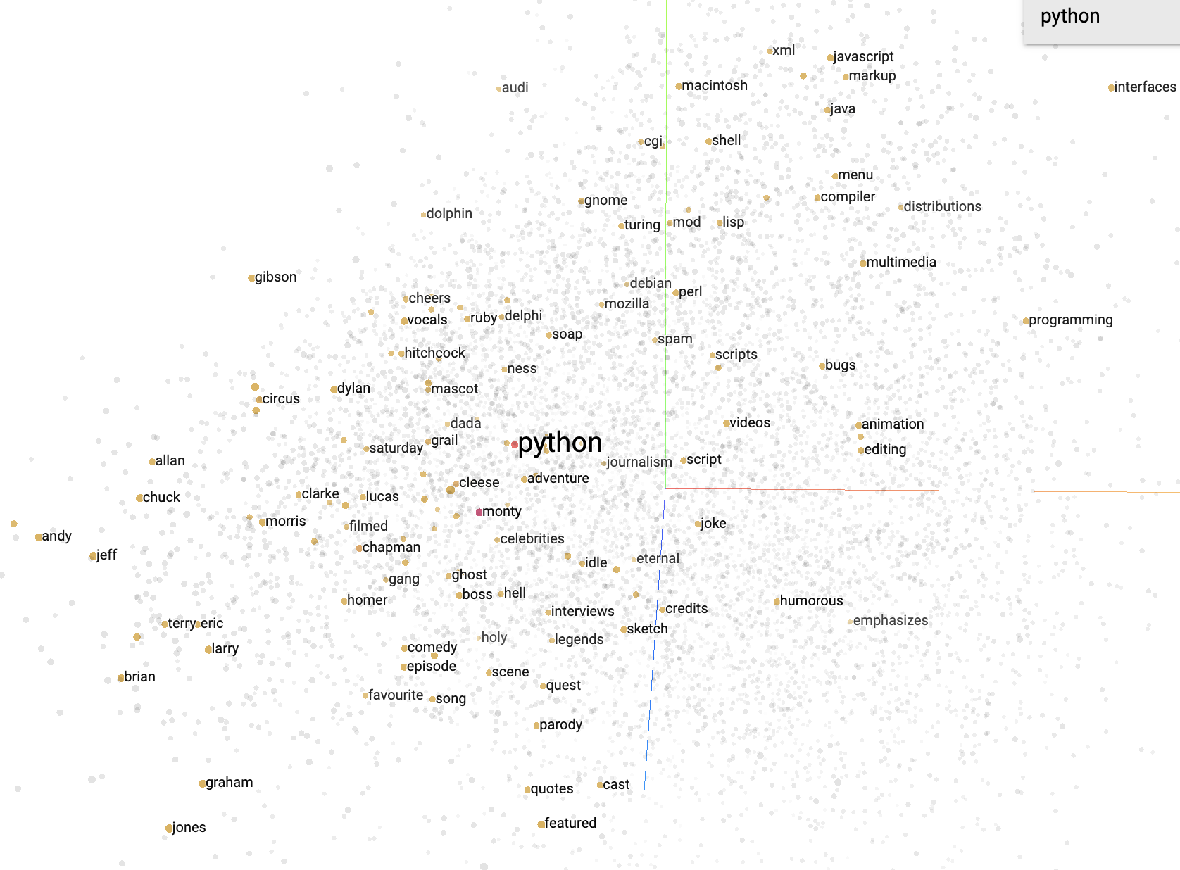
In an immense oversimplification, the process used for word embeddings is to read in a large amount of text and then use machine learning algorithms to determine similarity by using the words around each word. This impacts general users like us in search engines, streaming services, dating applications, and much more! For example, if you were to search Python topics in your search results may appear referring to the coding language, the reptile, the comedy troupe, and many more. When we use machine learning to determine word meanings, it is important that the data is first parsed correctly and stored in efficient ways so that we can access elements as needed. Understanding how to work with strings and problems that can arise with them is important to utilizing text successfully.
Reference: https://projector.tensorflow.org/
Strings are data structures which store an ordered set of characters. Recall that a character can be a: letter, number, symbol, punctuation mark, or white space. Strings can contain any number and any combination of these. As such, strings can be single characters, words, sentences, and even more.
Let’s refresh ourselves on how strings work, starting with the example string: s = "Go Cats!".
| Character | G | o | C | a | t | s | ! | |
| Index | 0 | 1 | 2 | 3 | 4 | 5 | 6 | 7 |
As with other data structures, we can access elements within the string itself. Using the example above, s[0] would contain the character ‘G’, s[1] would contain the character ‘o’, s[2] would contain the character ’ ‘, and so on.
We can determine the size of a string by using length functions; in our example, the length of s would be 8. It is also important to note that when dealing with strings, null is not equivalent to “”. For string s = "", the length of s would be 0. However for string s = null, accessing the length of s would return an error that null has no length property.
We can also add to strings or append on a surface level; though it is not that simple behind the scenes. The String class is immutable. This means that changes will not happen directly to the string; when appending or inserting, code will create a new string to hold that value. More concisely, the state of an immutable object cannot change.
We cannot assign elements of the string directly and more broadly for any immutable object. For example, if we wanted the string from our example to be ‘Go Cat!!’, we cannot assign the element through s[6] = '!'. This would result in an item assignment error.
For an example, consider string s = ‘abc’. If we then state in code s = s + ‘123’, this will create a new place in memory for the new definition of s. We can verify this in code by using the id() function.
string s = 'abc'
id(s)
Output: 140240213073680 #may be different on your personal device

string s = s + '123'
id(s)
Output: 140239945470168
While on the surface it appears that we are working with the same variable, our code will actually refer to a different one. There are many other immutable data types as well as mutable data types.
On the topic of immutable, we can also discuss the converse: mutable objects. Being a mutable object means that the state of the object can change. In CC310, we often worked with arrays to implement various data structures. Arrays are mutable, so as we add, change, or remove elements from an array, the array changes its state to accommodate the change rather than creating a new location in memory.
| Data Type | Immutable? |
|---|---|
| Lists | ☐ |
| Sets | ☐ |
| Byte Arrays | ☐ |
| Dictionaries | ☐ |
| Strings | ☑ |
| Ints | ☑ |
| Floats | ☑ |
| Booleans | ☑ |
Reference: http://people.cs.ksu.edu/~rhowell/DataStructures/strings/strings.html
Consider the following block of pseudocode:
1. function APPENDER(NUMBER, BASE)
2.     RESULT = ""
3.     loop I from 1 to NUMBER
4.         RESULT = RESULT + BASE
5.         if I MOD 2 = 0
6.             RESULT = RESULT + " "
7.         else
8.             RESULT = RESULT + ", "
9.     end loop
10.    return RESULT
11. end function
Lets step through the function call with APPENDER(4,'abc') and analyze the memory that the code takes.
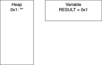
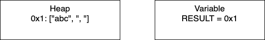
Recall that strings are reference variables. As such, string variables hold pointers to values and the value is stored in memory. For the following example, the HEAP refers to what is currently stored in memory and VARIABLE shows the current value of the variable RESULT.
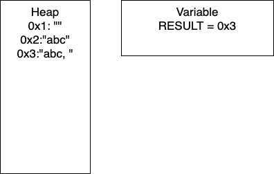
Initialization: In line two, we initialize RESULT as an empty string. In the heap, we have the empty string at memory location 0x1. Thus, RESULT is holding the pointer 0x1.
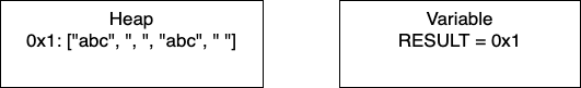
I = 1: Now we have entered the loop and on line 4, we add more characters to our string. At this point, we would have entry 0x2 in our heap and our variable RESULT would have the pointer 0x2. Continuing through the code, line 5 determines if I is divisible by 2. In this iteration I = 1, so we take the else branch. We again add characters to our string, resulting in a new entry in 0x3 and our variable RESULT containing the pointer 0x3. In total, we have written 8 characters. We then increment I and move to the next iteration.
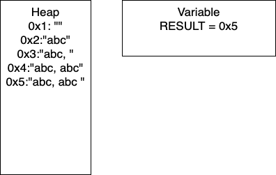
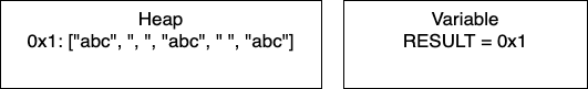
I = 2: We continue the loop and on line 4, we add more characters to our string. At this point, we would have entry 0x4 in our heap and our variable RESULT would have the pointer 0x4. Continuing through the code, line 5 determines if I is divisible by 2. In this iteration I = 2, so we take the if branch. We again add characters to our string, resulting in a new entry in 0x5 and our variable RESULT containing the pointer 0x5. In this iteration, we have written 17 characters. We then increment I and move to the next iteration of the loop.
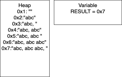
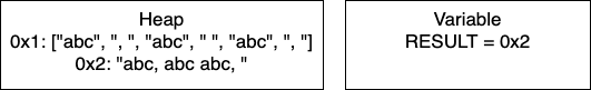
I = 3: We continue the loop and on line 4, we add more characters to our string. At this point, we would have entry 0x6 in our heap and our variable RESULT would have the pointer 0x6. Continuing through the code, line 5 determines if I is divisible by 2. In this iteration I = 3, so we take the if branch. We again add characters to our string, resulting in a new entry in 0x7 and our variable RESULT containing the pointer 0x7. In this iteration, we have written 26 characters. We then increment I and thus I = 4 breaking out of the loop.
We can do some further analysis of the memory that is required for this particular block.
| Iteration | Memory Entries | Total Character Copies |
|---|---|---|
| 1 | 3 | 8 |
| 2 | 5 | 8 + 17 = 25 |
| 3 | 7 | 25 + 26 = 51 |
| 4 | 9 | 51 + 35 = 86 |
| . | . | . |
| n | 2n + 1 | (9n2 + 7n)/2 |
You need not worry about creating the equations! Based on this generalization, if the user wanted to do 100K iterations, say for gene sequencing, there would be (2x100,000 - 1) = 200,001 memory entries and (9x100,0002 + 7x100,000)/2 = 45 billion character copies. This behavior is not exclusive to strings; this will occur for any immutable type.
While this example is contrived, it is not too far off the mark. Another caveat to this analysis is that, depending on our programming language, there will be a periodic ‘memory collection’; there wont be 200K memory addresses occupied at one time. Writing to memory in this way can be costly in terms of time, which in industry is money.
As a result of being immutable, strings can be cumbersome to work with in certain applications. When working with long strings or strings that we are continually appending to, such as in the memory example, we end up creating a lot of sizable copies.
Recall from the memory example the block of pseudocode.
1. function APPENDER(NUMBER, BASE)
2.     RESULT = ""
3.     loop I from 1 to NUMBER
4.         RESULT = RESULT + BASE
5.         if I MOD 2 = 0
6.             RESULT = RESULT + " "
7.         else
8.             RESULT = RESULT + ", "
9.     end loop
10.    return RESULT
11. end function
In this example, what if we changed RESULT to a mutable type, such as a StringBuilder in Java. Once the loop is done, we can cast RESULT to a string. By changing just the one aspect of the code, we would make only one copy of RESULT and have far less character copies.
Java specifically has a StringBuilder class which was created for this precise reason.
Consider the following, and note the slight changes on lines 2, 4, 6, 8 and the additional line 10.
1. function APPENDER_LIST(NUMBER, BASE)
2.     RESULT = []
3.     loop I from 1 to NUMBER
4.         RESULT.APPEND(BASE)
5.         if I MOD 2 = 0
6.             RESULT.APPEND(" ")
7.         else
8.             RESULT.APPEND(", ")
9.     end loop
10.    RESULT = "".JOIN(RESULT)
11.    return RESULT
12. end function
Now consider APPENDER_LIST(4,‘abc’)
Initialization: We start by initializing the empty array. RESULT will hold the pointer 0x1.
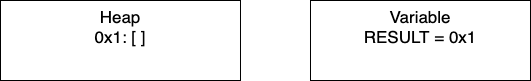
I = 1: Now we have entered the loop and on line 4, we add more characters to our array. At this point, we would have only entry 0x1 in our heap and our variable RESULT would have the pointer 0x1. Continuing through the code, line 5 determines if I is divisible by 2. In this iteration I = 1, so we take the else branch. We again add characters to our array. In total, we have written 5 characters. We then increment I and move to the next iteration.
I = 2: We continue the loop and on line 4, we add more characters to our array. We still have just one entry in memory and our pointer is still 0x1. In this iteration, we have written 4 characters. We then increment I and move to the next iteration of the loop.
I = 3: We continue the loop and on line 4, we add more characters to our array. In this iteration, we have written 5 characters. We then increment I and thus I = 4 breaking out of the loop.
Post-Loop: Once the loop breaks, we join the array to create the final string. This creates a new place in memory and changes RESULT to contain the pointer 0x2.
We can do some further analysis of the memory that is required for this particular block.
| Iteration | Memory Entries | Character Copies |
|---|---|---|
| 1 | 2 | 8 |
| 2 | 2 | 17 |
| 3 | 2 | 26 |
| 4 | 2 | 35 |
| . | . | . |
| n | 2 | 9n - 1 |
Again, you need not worry about creating these equations for this course. To illustrate the improvement even more explicitly, let’s consider our previous example with 100K iterations. For APPENDER there were (2x100,000 - 1) = 200,001 memory entries and (9x100,0002 + 7x100,000)/2 = 45 billion character copies. For APPENDER_LIST we now have just 2 memory entries and (9x100,000 - 1) = 899,999 character copies. This dramatic improvement was a result of changing our data structure ever so slightly.
Reference: http://people.cs.ksu.edu/~rhowell/DataStructures/strings/stringbuilders.html
In this module, we reviewed each of the data structures we have explored in this class. Most importantly, we looked at how they compare in terms of performance and discussed some of the best and most efficient ways to use them in our programs.
Using that information, we introduced the standard collection libraries for both Java and Python, and saw how those professional implementations closely follow the same ideas and analysis that we saw in our own structures. While the professional structures may have many more features and more complex code, at the core they still work just like the structures we learned how to build from scratch.
One of the best traits of a good programmer is knowing how to most effectively use the tools made available to us through the programming languages and libraries we have chosen to use. The goal of this class is to give us the background we need to understand how the various collection data structures we can choose from work, so that we can use them in the most effective way to build useful and efficient programs.
YouTube VideoTo start this course, we have looked into strings. They are a very natural way to represent data, especially in real world applications. Often though, the datapoints can be very large and require multiple modifications. We also examined how strings work: element access, retrieving the size, and modifying them. We looked into some alternatives which included StringBuilders for Java and character arrays for Python.
To really understand this point, we have included a comparison. We have implemented the APPENDER and APPENDER_LIST functions in both Python and Java. For the Java implementation, we utilized StringBuilders.
1. function APPENDER(NUMBER, BASE)
2.     RESULT = ""
3.     loop I from 1 to NUMBER
4.         RESULT = RESULT + BASE
5.         if I MOD 2 = 0
6.             RESULT = RESULT + " "
7.         else
8.             RESULT = RESULT + ", "
9.     end loop
10.    return RESULT
11. end function
1. function APPENDER_LIST(NUMBER, BASE)
2. RESULT = []
3. loop I from 1 to NUMBER
4. RESULT.APPEND(BASE)
5. if I MOD 2 = 0
6. RESULT.APPEND(" ")
7. else
8. RESULT.APPEND(", ")
9. end loop
10. RESULT = "".JOIN(RESULT)
11. return RESULT
12. end functionFor the tests of 108 and 109 in Java, the string implementation took over 24 hours and the StringBuilder implementation ran out of memory. For these reasons, they are omitted from the figure.
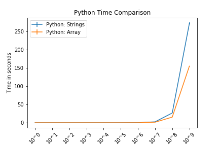
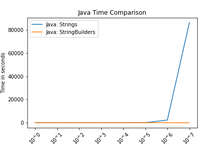
These figures compare Strings and lists for Python and Strings and StringBuilders for Java. The intention of these is not to compare Python and Java.
In both languages, we see that the string function and the respective alternative performed comparably until approximately 106 (1,000,000 characters). Again, these are somewhat contrived examples with the intention of understanding side effects of using strings.
As we have discussed, modern coding languages will have clean up protocols and memory management strategies. With the intention of this class in mind, we will not discuss the memory analysis in practice.
When modifying strings we need to be cognizant of how often we will be making changes and how large those changes will be. If we are just accessing particular elements or only doing a few modifications then using plain strings is a reasonable solution. However, if we are looking to build our own DNA sequence this is not a good way to go as strings are immutable.
