Chapter 11
Graph Algorithms
Algorithms for working with graphs!
Algorithms for working with graphs!
In the previous modules, we have introduced graphs and two implementations. This module will cover the traversals through graphs as well as path search techniques.
As we have discussed previously, graphs can have many applications. Based on that, there are many things that we may want to infer from graphs. For example, if we have a graph that depicts a railroad or electrical network, we could determine what maximum flow of the network. The standard approach for this task is the Ford-Fulkerson Algorithm. In short, given a graph with edge weights that represent capacities the algorithm will determine the maximum flow throughout the graph.
From the matrix graph module, we used the following distribution network as an example.

Conceptually, we would want to determine the maximum number of units that could leave the distribution center without having excess laying around stores. Using the maximum flow algorithm, we would determine that the maximum number of units would be 15.

The driving force in the Ford-Fulkerson algorithm, as well as other maximum flow algorithms, is the ability to find a path from a source to a target. Specifically, these algorithms use breadth first and depth first searches to discover possible paths.
To get to introducing the searches, we will first discuss the basis of them. Those are the depth first traversal and the breadth first traversal. We will outline the premise of these traversals and then discuss how we can modify their algorithms for various tasks, such as path searches.
We can perform these traversals on any type of graph. Conceptually, it will help to have a tree-like structure in mind to differentiate between depth first and breadth first.

First we will discuss Depth First Traversal. We can define the depth first traversal in two ways, iteratively or recursively. For this course, we will define it iteratively.
In the iterative algorithm, we will initialize an empty stack and an empty set. The stack will determine which node we search next and the set will track which nodes we have already searched.
Recall that a stack is a ‘Last In First Out’ (LIFO) structure. Based on this, the depth first traversal will traverse a nodes descendants before its siblings.
To do the traversal, we must pick a starting node; this can be an arbitrary node in our graph. If we were doing the traversal on a tree, we would typically select the root at a starting point. We start a while loop to go through the stack which we will be pushing and popping from. We get the top element of the stack, if the node has not been visited yet then we will add it to the set to note that we have now visited it. Then we get the neighbors of the node and put them onto the stack and continue the process until the stack is empty.
function DEPTHFIRST(GRAPH,SRC)
    STACK = empty array
    DISCOVERED = empty set
    append SRC to STACK
    while STACK is not empty
        CURR = top of the stack
        if CURR not in DISCOVERED
            add CURR to DISCOVERED
            NEIGHS = neighbors of CURR
            for EDGE in NEIGHS
                NODE = first entry in EDGE
                append NODE to STACK
Since the order of the neighbors is not guaranteed, the traversal on the same graph with the same starting node can find nodes in different orders.
We can also perform a breadth first traversal either iteratively or recursively. As with the depth first traversal, we will define it iteratively.
In the iterative algorithm, we initialize an empty queue and an empty set. Like depth first traversal, the set will track which nodes we have discovered. We now use a queue to track which node we will search next.
Recall that a queue is a ‘First In First Out’ (FIFO) structure. Based on this, the breadth first traversal will traverse a nodes siblings before its descendants.
Again, we must pick a starting node; this can be an arbitrary node in our graph. We add the starting node to our queue and the set of discovered nodes. We start a while loop to go through the queue which we will be enqueue and dequeue from. We get the first element of the queue, then get the neighbors of the current node. We loop through each edge adding the neighbor to the discovered set and the queue if it has not already been discovered. We continue this process until the queue is empty.
function BREADTHFIRST(GRAPH,SRC)
    QUEUE = empty queue
    DISCOVERED = empty set
    add SRC to DISCOVERED
    add SRC to QUEUE
    while QUEUE is not empty
        CURR = first element in QUEUE
        NEIGHS = neighbors of CURR
        for EDGE in NEIGHS
            NODE = first entry in EDGE
            if NODE is not in DISCOVERED
                add NODE to DISCOVERED
append NODE to QUEUEIt is important to remember in these implementations that a stack is used for depth first and a queue is used for a breadth first. The stack, being a LIFO structure, will proceed with the newest entry which will put us farther away from the source. The queue, being a FIFO structure, will proceed with oldest entry which will focus the algorithm more on the adjacent nodes. If we were to use say a queue for a depth first search, we would be traversing neighbors before descendants.
When introducing graphs, we discussed how the components of a graph didn’t have to all be connected. If our goal is to visit each node, like in the searches, then we will need to perform the search from every node.
For example, the graph below has two separate components. Lets walk through which nodes we will discover by calling the traversals from each node.

| Start | Visited (in alphabetical order) |
|---|---|
| A | {A, D, H} |
| B | {B, E, H, I} |
| C | {C} |
| D | {D} |
| E | {E, H, I} |
| F | {C, F} |
| G | {C, G} |
| H | {H} |
| I | {I} |
| J | {C, F, G, J} |
In this example, we would need to call either traversal on nodes A, B and J in order to visit all of the nodes.
An important application for these traversals is the ability to find a path between two nodes. This has many applications in railroad networks as well as electrical wiring. With some modifications to the traversals, we can determine if electricity can flow from a source to a target. We will modify depth first and breadth first traversals in similar ways.
There are three cases that can happen when we search for a path between nodes:
With these searches, we are not guaranteed to return the same path if there are multiple paths.
We will call these Depth First Search (DFS) and Breadth First Search (BFS). In both traversals, we have added the following extra lines: 4, 9-16, and 22 through the end.
First, we have the addition of PARENT_MAP which will be a dictionary to keep track of how we get from one node to another. We will use the convention of having the key be the child and the value be the parent. While we use the terms child and parent, this is not exclusive to trees.
The ending portion starting at line 22, will add entries to our dictionary. If we haven’t already found an edge to NODE, then we will add the edge that we are currently on.
The other addition is the block of code from line 9 to 16. We will enter this if block if the node that we are currently at is the target. This means that we have finally found a path from the source node to the target node. The process in this segment of code will backtrack through the path and build the path.
 1function DEPTHFIRSTSEARCH(GRAPH,SRC,TAR)
 2    STACK = empty array
 3    DISCOVERED = empty set
 4    PARENT_MAP = empty dictionary
 5    append SRC to STACK
 6    while STACK is not empty
 7        CURR = top of the stack
 8        if CURR not in DISCOVERED
 9            if CURR is TAR
10                 PATH = empty array
11                 TRACE = TAR
12                 while TRACE is not SRC
13                     append TRACE to PATH
14                     set TRACE equal to PARENT_MAP[TRACE]
15                 reverse the order of PATH
16                 return PATH
17            add CURR to DISCOVERED
18            NEIGHS = neighbors of CURR
19            for EDGE in NEIGHS
20                NODE = first entry in EDGE
21                append NODE to STACK
22                if PARENT_MAP does not have key NODE
23                    in the PARENT_MAP dictionary set key NODE with value CURR
24    return nothing
 1function BREADTHFIRSTSEARCH(GRAPH,SRC,TAR)
 2    QUEUE = empty queue
 3    DISCOVERED = empty set
 4    PARENT_MAP = empty dictionary
 5    add SRC to DISCOVERED
 6    add SRC to QUEUE
 7    while QUEUE is not empty
 8        CURR = first element in QUEUE
 9        if CURR is TAR
10            PATH = empty list
11            TRACE = TAR
12            while TRACE is not SRC
13                    append TRACE to PATH
14                    set TRACE equal to PARENT_MAP[TRACE]
15                reverse the order of PATH
16                return PATH
17        NEIGHS = neighbors of CURR
18        for EDGE in NEIGHS
19            NODE = first entry in EDGE
20            if NODE is not in DISCOVERED
21                add NODE to DISCOVERED
22                if PARENT_MAP does not have key NODE
23                    in the PARENT_MAP dictionary set key NODE with value CURR
24                append NODE to QUEUE
25    return nothing
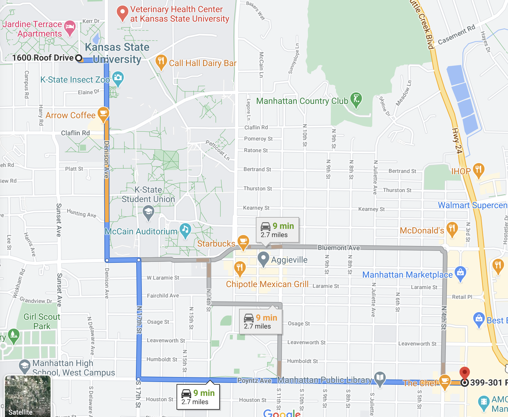
Finding a path in a graph is a very common application in many fields. One application that we benefit from in our day to day lives is traveling. Programs like Google Maps calculate various paths from point A to point B.
In the context of graph data structures, we can think of each intersection as a node and each road as an edge. Google Maps, however, tracks more features of edges than we have discussed. Not only do they track the distance between intersections, they also track time, tolls, construction, road surface and much more. In the next module, we will discuss more details of how we can find the shortest path.
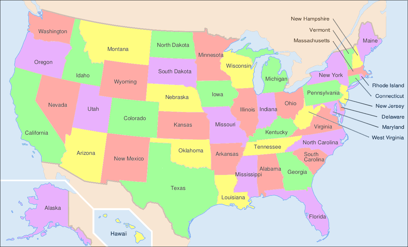
Another application of the general searches is coloring maps. The premise is that we don’t want two adjacent territories to have the coloring. These territories could be states, like in the United States map below, counties, provinces, countries, and much more.
The following was generated for this course using the breadth first search and MyMatrixGraph class that we have implemented in this course. To create the visual rendering, the Python library NetworkX^[https://networkx.github.io/] was used. In this rendering, the starting node was Utah. If we were to start from say Alabama or Florida, we would not have a valid four coloring scheme once we got to Nevada. Since Hawaii and Alaska have no land border with any of the states, they can be any color.
We will continue to work with graph algorithms in this module, specifically with finding minimum spanning trees (MST). MSTs have many real world applications such as:
Suppose we were building an apartment complex and wanted to determine the most cost-effective wiring schema. Below, we have the possible construction costs for wiring apartment to apartment. Wiring vertically adjacent apartments is cheaper than wiring horizontally adjacent units and those closest to the power closet have lower costs as well.

To find the best possible solution, we would find the MST. The final wiring schema may look something like the figure below.

Determining a MST can result in lower costs and time used in many applications, especially logistics. To properly define a minimum spanning tree, we will first introduce the concept of a spanning tree.
A spanning tree for a graph is a subset of the graphs edges such that each node is visited once, no cycles are present, and there are no disconnected components.
Let’s look at this graph as an example. We have five nodes and seven edges.

Below, we have valid examples of spanning trees. In each of the examples, we visit each node and there are no cycles. Recall that a cycle is a path in which the starting node and ending node are the same.

To be a spanning tree of a graph, it must:
Further, we can imagine selecting a node in a spanning tree as the root and letting gravity take effect. This gives us a visual motivation as to why they are called spanning trees. In these examples, we have selected node A for the root for each of the spanning trees above.

Below, we have invalid examples of spanning trees. In the left column, the examples are where all of the nodes are not connected in the same component. In the right column, the examples contain cycles. For example in the top right, we have the cycle B->C->D->E->B

Now that we have an understanding of general spanning trees, we will introduce the concept of minimum spanning trees. First let’s introduce the concept of the cost of a tree.
The cost that is associated with a tree, is the sum of its edges weights. Let’s look at this spanning tree which is from the previous page. The cost associated with this spanning tree is: 2+6+10+14=32.

A minimum spanning tree is a spanning tree that has the smallest cost. Recall the graph from the previous page.
Below on the left is a minimum spanning tree for the graph above. On the right is an example of a spanning tree, though it does not have the minimum cost.

In this small example, it is rather straightforward to find the minimum spanning tree. We can use a bit of trial and error to determine if we have the minimum spanning tree or not. However, once the graphs start to get more nodes and more edges it quickly becomes more complicated.

There are two algorithms that we will introduce to give us a methodical way of finding the minimum spanning tree. The first that we will look at is Kruskal’s algorithm and then we will look at Prim’s algorithm.
As graphs get larger, it is important to go about finding the MST in a methodical way. In the mid 1950’s, there was a desire to form an algorithmic approach for solving the ’traveling salesperson’ problem^[We will describe this problem in a future section of this module]. Joseph Kruskal first published this algorithm in 1956 in the Proceedings of the American Mathematical Society1. The algorithms prior to this were, as Kruskal said, “unnecessarily elaborate” thus the need for a more succinct algorithm arose.
In his original work, Kruskal outlined three different yet similar algorithms to finding a minimum spanning tree. The Kruskal Algorithm that we use is as follows:
u and v are connected by the edge and they are not in the same set yet, then join the two sets and add the edge to your set of edges

function KRUSKAL(GRAPH)
    MST = GRAPH without the edges attribute(s)
    ALLSETS = an empty list which will contain the sets
    for NODE in GRAPH NODES
        SET = a set with element NODE
        add SET to ALLSETS
    EDGES = list of GRAPH's edges
    SORTEDEDGES = EDGES sorted by edge weight, smallest to largest
    for EDGE in SORTEDEDGES
        SRC = source node of EDGE
        TAR = target node of EDGE
        SRCSET = the set from SETS in which SRC is contained
        TARSET = the set form SETS in which TAR is contained
        if SRCSET not equal TARSET
            UNIONSET = SRCSET union TARSET
            add UNIONSET to ALLSETS
            remove SRCSET from ALLSETS
            remove TARSET from ALLSETS
            add EDGE to MST as undirected edge
return MSTThe history of Prim's Algorithm is not as straight forward as Kruskal’s. While we often call it Prim's Algorithm, it was originally developed in 1930 by Vojtěch Jarník. Robert Prim later rediscovered and republished this algorithm in 1957, one year after Kruskals. To add to the naming confusion, Edsger Dijkstra also published this work again in 1959. Because of this, the algorithm can go by many names: Jarkík's Algorithm, Jarník-Prim's Algorithm, Prim-Dijkstra's Algorithm, and DJP Algorithm.
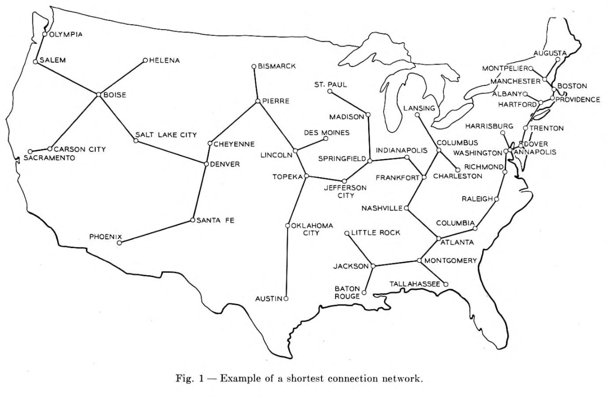
Prim cited “large-scale communication” as the motivation for this algorithm, specifically the “Bell System leased-line”1. Leased lines were used primarily in a commercial setting which connected business offices that were geographically distant (IE in different cities or even states). Companies would want all offices to be connected but wanted to avoid having to lay an excessive amount of wire. Below is a figure which Prim used to motivate the need for the algorithm. This image depicts the minimum spanning tree which connect each of the US continental state capitals along with Washington D.C.
The basis of the algorithm is to start with only the nodes of the graph, then we do the following

Uniqueness
You may have noticed that the minimum spanning tree that resulted from Kruskal’s algorithm differed from Prim’s algorithm. We have displaying them both below for reference.
| Kruskal | Prim |
|---|---|
|
|
|
While these are different, they are both valid. The trees both have cost 16. The MST of a graph will be unique, meaning there is only one, if none of the edges of the graph have the same weight.
function PRIM(GRAPH, START)
    MST = GRAPH without the edges attribute(s)
    VISITED = empty set
    add START to VISITED
    AVAILEDGES = list of edges where START is the source
    sort AVAILEDGES
    while VISITED is not all of the nodes
        SMLEDGE = smallest edge in AVAILEDGES
        SRC = source of SMLEDGE
        TAR = target of SMLEDGE
        if TAR not in VISITED
            add SMLEDGE to MST as undirected edge
            add TAR to VISITED
            add the edges where TAR is the source to AVAILEDGES
        remove SMLEDGE from AVAILEDGES
        sort AVAILEDGES
    return MST
R.C. Prim, May 8, 1957 Shortest Connection Networks And Some Generalizations https://archive.org/details/bstj36-6-1389 ↩︎
While we won’t outline algorithms suited for solving the traveling salesperson problem (TSP), we will outline the premise of the problem. This problem was first posed in 1832, almost a two centuries ago, and is still quite prevalent. It is applicable to traveling routes, distribution networks, computer architecture and much more. The TSP is a seminal problem that has motivated many research breakthroughs, including Kruskal’s algorithm!
The motivation of the TSP is this: given a set of locations, what is the shortest path such that we can visit each location and end back where started?
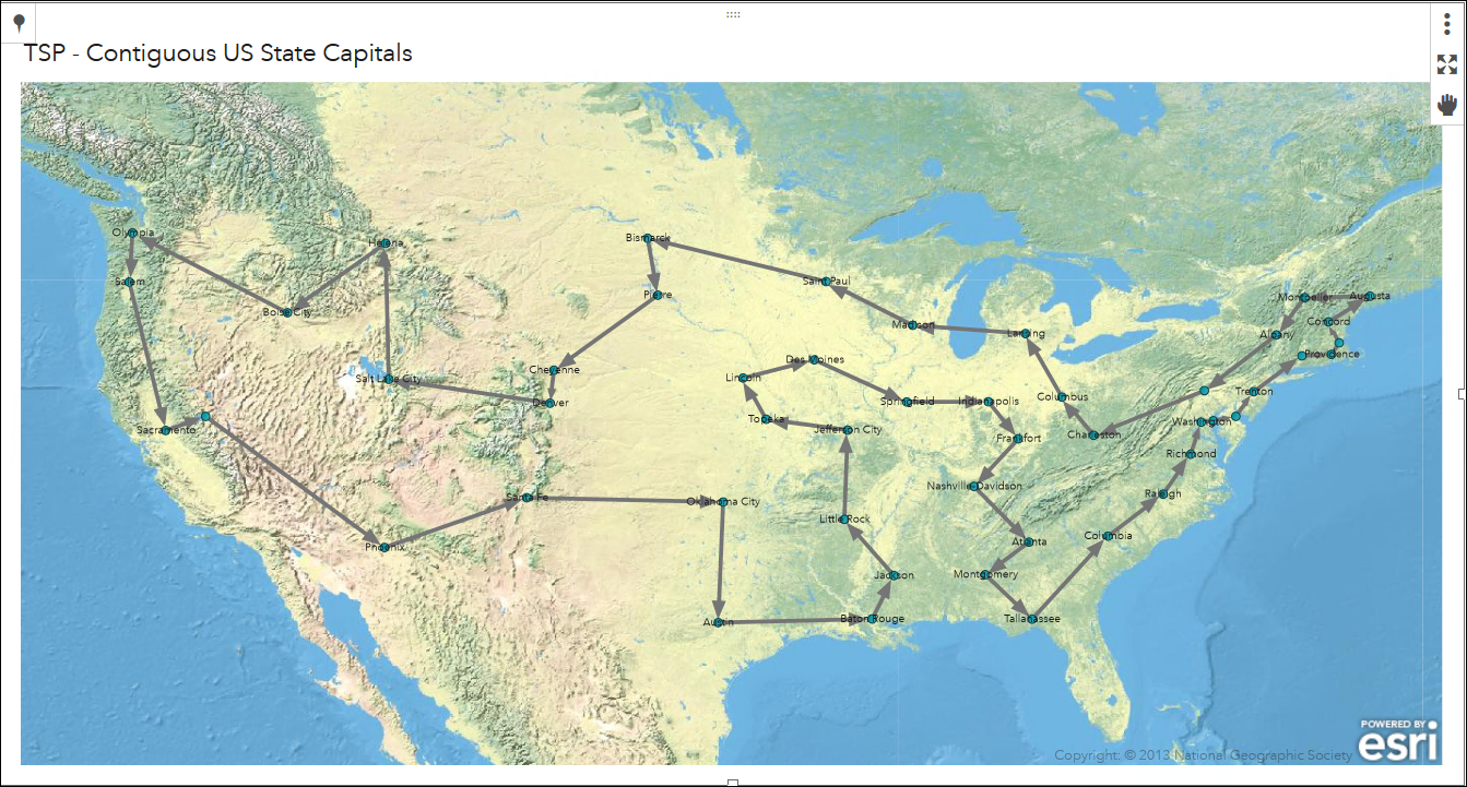
Suppose we wanted to take a road trip with friends to every state capital in the continental US as well as Washington D.C. To save money and time, we would want to minimize the distance that we travel. Since we are taking a road trip, we would want to avoid frivolous driving. For example, if we start in Sacremento, CA we would not want to end the trip in Boston, MA. The trip should start and end at the same location for efficiency.
The figure below shows the shortest trip that visits each state capital and Washington D.C. once. In this example, we can start where ever we like and will end up where we started.
In this problem, it is easy to get overwhelmed by all of the possibilities. Since there are 49 cities to visit, there are over 6.2*10^60 possibilities. For reference, 10^12 is equivalent to one trillion! Thus, we need an algorithmic approach to solve this problem as opposed to a brute force method.