Welcome!
This page is the main page for Performance
This page is the main page for Performance
There are several linear data structures that we can use in our programs, including stacks, queues, lists, sets, and hash tables. In this course, we have covered each of these structures in detail. However, as a programmer, one of the most difficult decisions we will make when developing a program is the choice of which data structure to use. Sometimes the choice may be obvious based on the data we plan to store or the algorithms we need to perform, but in practice that happens very rarely. Instead, we are faced with competing tradeoffs between various factors such as ease of use, performance, and simplicity.
In this chapter, we’ll review the various data structures and algorithms we’ve learned about in this course, but this time we’ll add a bit more focus on the decisions a programmer would make when choosing to use a particular data structure or algorithm.
The choice of which data structure to use is often the most consequential choice we make when developing a new piece of software, as it can have a large impact on the overall performance of the program. While there are many different factors to consider, here are three important questions we can ask when choosing a data structure:
By answering the questions above in the order they are presented, we should be able to make good decisions about which data structures would work best in our program. We are purposely putting more focus on writing working and understandable code instead of worrying about performance. This is because many programs are only used with small data sets on powerful modern computers, so performance is not the most important aspect. However, there are instances where performance becomes much more important, and in those cases more focus can be placed on finding the most performant solution as well.
As it turns out, these three questions are very similar to a classic (trilemma)[https://en.wikipedia.org/wiki/Trilemma] from the world of business, as shown in the diagram below.
 ^[File:Project-triangle.svg. (2020, January 12). Wikimedia Commons, the free media repository. Retrieved 21:09, April 30, 2020 from https://commons.wikimedia.org/w/index.php?title=File:Project-triangle.svg&oldid=386979544.]
In the world of software engineering, it is said that the process of developing a new program can only have two of the three factors of “good”, “fast”, and “cheap”. The three questions above form a similar trilemma. Put another way, there will always be competing tradeoffs when selecting a data structure for our programs.
For example, the most performant option may not be as easy to understand, and it may be more difficult to debug and ensure that it works correctly. A great example of this is matrix multiplication, a very common operation in the world of high-performance computing. A simple solution requires just three loops and is very easy to understand. However, the most performant solution requires hundreds of lines of code, assembly instructions, and a deep understanding of the hardware on which the program will be executed. That program will be fast and efficient, but it is much more difficult to understand and debug.
Data structures that are used in our programs can be characterized in terms of two performance attributes: processing time and memory usage.
We will not worry about memory usage at this point, since most of the memory used in these data structures is consumed by the data that we are storing. More technically, we would say that the memory use of a data structure containing N elements is on the order of $N$ size. However, some structures, such as doubly linked lists, must maintain both the next and previous pointers along with each element, so there can be a significant amount of memory overhead. That is something we should keep in mind, but only in cases where we are dealing with a large amount of data and are worried about memory usage.
When evaluating the processing time of a data structure, we are most concerned with the algorithms used to add, remove, access, and find elements in the data structure itself. There are a couple of ways we can evaluate these operations.
Throughout this course, we have included mathematical descriptions of the processing time of most major operations on the data structures we have covered.
One of the best ways to compare data structures is to look at the common operations that they can perform. For this analysis, we’ve chosen to analyze the following four operations:
The following table compares the best- and worst-case processing time for many common data structures and operations, expressed in terms of $N$, the number of elements in the structure.
| Data Structure | Insert Best | Insert Worst | Access Best | Access Worst | Find Best | Find Worst | Delete Best | Delete Worst |
|---|---|---|---|---|---|---|---|---|
| Unsorted Array | $1$ | $1$ | $1$ | $1$ | $N$ | $N$ | $N$ | $N$ |
| Sorted Array | $\text{lg}(N)$ | $N$ | $1$ | $1$ | $\text{lg}(N)$ | $\text{lg}(N)$ | $\text{lg}(N)$ | $N$ |
| Array Stack (LIFO) | $1$ | $1$ | $1$ | $1$ | $N$ | $N$ | $1$ | $1$ |
| Array Queue (FIFO) | $1$ | $1$ | $1$ | $1$ | $N$ | $N$ | $1$ | $1$ |
| Unsorted Linked List | $1$ | $1$ | $N$ | $N$ | $N$ | $N$ | $N$ | $N$ |
| Sorted Linked List | $N$ | $N$ | $N$ | $N$ | $N$ | $N$ | $N$ | $N$ |
| Linked List Stack (LIFO) | $1$ | $1$ | $1$ | $1$ | $N$ | $N$ | $1$ | $1$ |
| Linked List Queue (FIFO) | $1$ | $1$ | $1$ | $1$ | $N$ | $N$ | $1$ | $1$ |
| Hash Table | $1$ | $N$ | $1$ | $N$ | $N$ | $N$ | $1$ | $N$ |
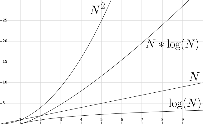
We can also compare these processing times by graphing the equations used to describe them. The graph below shows several of the common orders that we have seen so far.
On the next few pages, we will discuss each data structure in brief, using this table to compare the performance of the various data structures we’ve covered in this course.
An unsorted array is the most basic data structure, and it is supported by nearly every programming language available. Inserting elements into the array is always a constant time operation since we can simply place it at the end of the array. Of course, this assumes that the array is large enough to hold all our data without needing to be resized. Since we are not worried about memory usage, this is a safe assumption.
Likewise, since an array allows us to access elements directly by index, we can say that the time it takes to access any single element is also a constant time operation.
Unfortunately, searching for an element is much more difficult. Since the array is unsorted, we would have to look through each element in the array to find a specific element, making the search operation run on the order of $N$ time.
Likewise, the process to find and delete a specific item from the list is also on the order of $N$ time, since we’d have to iterate through the list to find the element, remove it, and then shift all remaining elements forward one space in the array.
Unsorted arrays work best when we simply need to store and access data quickly, but we are not really concerned with finding a specific element each time. Iterating across an entire array takes the same amount of time as finding a specific element, so arrays are great data structures to use when looping through data. As we saw in a previous module, we can probably search linearly through the array for a specific item as many as 7 times before it becomes more efficient to sort it first.
We can improve on some aspects of the performance of an unsorted array by sorting it. Thankfully, we can make it easier by just sorting the data as we insert it into the array! However, by doing so, our insert operation now runs in the order of $\text{lg}(N)$ time in the best case. This is because it must use a binary search process to figure out where to insert the data into the array. However, in the worst case, it must also shift all the elements after the inserted element back one space, which will make the insert operation run in the order of $N$ time.
Thankfully, since the data is being stored in an array, we can still use array indexes to access single elements directly, making that operation constant time. In addition, now that the array is sorted, the process of finding a specific element is reduced to the order of $\text{lg}(N)$ time, a vast improvement over the performance of an unsorted array.
Finally, the process of finding and deleting a specific item can be improved to order of $\text{lg}(N)$ time in the best case, but the worst case once again involves shifting all of the elements in the array, which is on the order of $N$ time.
So, while having a sorted array allows us to improve the performance of finding specific elements, many of the other operations still have poor worst-case performance. Therefore, one of the important things we must consider when choosing whether to store data in a sorted or unsorted array is the number of times we’ll be searching for specific elements vs. the number of times we’ll just be inserting or iterating across the entire array. If we do more iterating, we may want to just use an unsorted array, but if we need to search for items repeatedly, a sorted array may be a better choice from a performance standpoint.
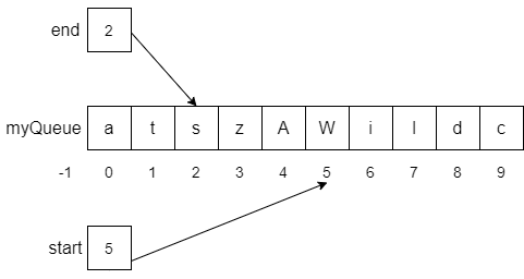
Our array-based implementations of a stack and a queue are very performant examples of data structures based on arrays, simply because we can limit the operations that we perform to the most efficient ones possible.
For example, since we are only inserting in one position, the insert operation always runs in constant time. While the position may be different depending on the implementation, each data structure simply keeps track of the array index where the next one should be placed, eliminating the need to shift elements around.
Likewise, since we are only allowed to remove elements from one position in the array, we can once again avoid the need to shift elements around. Therefore, that operation also runs in constant time for both stacks and queues.
We can also use the peek operation to access the next element in the stack or queue in constant time. Since it is array based, those operations only require the index of the element in the array to be known, which is a great advantage here.
However, the find operation still runs in order $N$ time, since it must iterate through each element in the array to determine if the desired element exists in the structure. Thankfully, that operation is not used very often with stacks and queues since we are usually concerned only with the next element to be taken from the structure.

The next data structure we learned about is the linked list. Specifically, we will look at the doubly linked list in this example, but in most instances the performance of a singly linked list is comparable.
With a linked list, the process of inserting an element at either the beginning or the end is a constant time operation since we maintain both a head and a tail reference. All we must do is create a new node and update a few references and we are good to go.
However, if we would like to access a specific element somewhere in the list, we will have to iterate through the list starting from either the head or the tail until we find the element we need. So, that operation runs in order $N$ time. This is the major difference between linked lists and arrays: with an array, we can directly access items using the array index, but with linked lists we must iterate to get to that element. This becomes important in the next section when we discuss the performance of a sorted linked list.
Similarly, the process of finding an element also requires iterating through the list, which is an operation that runs in order $N$ time.
Finally, if we want to find and delete an element, that also runs in order $N$ time since we must search through the list to find the element. Once we have found the element, the process of deleting that element is a constant time operation. So, if we use our list iterator methods in an efficient manner, the actual run time may be more efficient than this analysis would lead us to believe.

We have not directly analyzed the performance of a sorted linked list in this course, but hopefully the analysis makes sense based on what we have learned before. Since the process of iterating through a linked list runs in order of $N$ time, every operation required to build a sorted linked list is limited by that fact.
For example, if we want to insert an element into a list in sorted order, we must simply iterate through the list to find the correct location to insert it. Once we’ve found it, the process of inserting is actually a constant time operation since we don’t have to shift any elements around, but because we can’t use binary search on a linked list, we don’t have any way to take advantage of the fact that the list is sorted.
The same problem occurs when we want to search for a particular element. Since we cannot use binary search to jump around between various elements in the list, we are limited to a simple linear search process, which runs in order of $N$ time.
Likewise, when we want to search and delete an element from the list, we must once again iterate through the entire list, resulting in an operation that runs in order $N$ time.
So, is there any benefit to sorting a linked list? Based on this analysis, not really! The purpose of sorting a collection is simply to make searching for a particular element faster. However, since we cannot use array indices to jump around a list like we can with an array, we do not see much of an improvement.
However, in the real world, we can improve some of these linear algorithms by “short-circuiting” them. When we “short-circuit” an algorithm, we provide additional code that allows the algorithm to return early if it realizes that it will not succeed.
For example, if we are searching for a particular element in a sorted list, we can add an if statement to check and see if the current element is greater than the element we are searching for. If the list is sorted in ascending order, we know that we have gone past the location where we expected to find our element, so we can just return without checking the rest of the list. While this does not change the mathematical analysis of the running time of this operation, it may improve the real-world empirical analysis of the operation.
We already saw how to use the operations from a linked list to implement both a stack and a queue. Since those data structures restrict the operations we can perform a bit, it turns out that we can use a linked list to implement a stack and a queue with comparable performance to an array implementation.
For example, inserting, accessing, and removing elements in a stack or a queue based on a doubly linked list are all constant time operations, since we can use the head and tail references in a doubly linked list to avoid the need to iterate through the entire list to perform those operations. In fact, the only time we would have to iterate through the entire list is when we want to find a particular element in the stack or the queue. However, since we cannot sort a stack or a queue, finding an element runs in order $N$ time, which is comparable to an array implementation.
By limiting the actions we want to perform with our linked list, we can get a level of performance similar to an array implementation of a stack or a queue. It is a useful outcome that demonstrates the ability of different data structures to achieve similar outcomes.

Analyzing the performance of a hash table is a bit trickier than the other data structures, mainly due to how a hash table tries to use its complex structure to get a “best of both worlds” performance outcome.
For example, consider the insert operation. In the best case, the hash table has a capacity that is large enough to guarantee that there are not any hash collisions. Each entry in the array of the hash table will be an empty list and inserting an element into an empty list is done in constant time, so the whole operation runs in the order of constant time.
The worst case for inserting an item into a hash table would be when every element has the same hash, so every element in the hash table is contained in the same list. In that case, we must iterate through the entire list to make sure the key has not already been used, which would be in the order of $N$ time.
Thankfully, if we properly design our hash table such that the capacity is much larger than our expected size, and the hash function we use to hash our keys results in a properly distributed hash, this worst case scenario should happen very rarely, if ever. Therefore, our expected performance should be closer to constant time.
One important thing to remember, however, is that each operation in a hash table requires computing the hash of the key given as input. Therefore, while some operations may run in constant time, if the action of computing the hash is costly, the overall operation may run very slowly.
The analysis of the operation to access a single element in a hash table based on a given key is similar. If the hash table elements are distributed across the table, then each list should only contain a single element. In that case, we can just compute the hash of the key and determine if that key has been used in a single operation, which runs in the order of constant time.
In the worst case, however, we once again have the situation where all the elements have been placed in the same linked list. We would need to iterate through each element to find the one we are looking for. In that case, the operation would run in the order of $N$ time.
The operation for finding a specific element in a hash table is a bit unique. In this case, we are discussing looking for a particular value, not necessarily a particular key. That operation is discussed in the previous paragraph. For the operation, the only possible way forward is to iterate through each list in the hash table and perform a linear search for the requested value, which will always run in order $N$ time.
Finally, if we want to delete a single element from a hash table based on a given key, the analysis is the same as inserting or finding an element. In the best case, it runs in the order of constant time, but the worst case runs in the order of N time since we must iterate through an entire list of $N$ elements.
Even though a hash table has some very poor performance in the worst case, as discussed earlier those worst case situations are very rare, and as long as we are careful about how we manage the capacity of our hash table and how we compute the hash of our objects, we can expect to see operations running in near constant time during normal usage.
We can examine the performance of the algorithms we use in a similar manner. Once again, we are concerned with both the memory usage and processing time of the algorithm. In this case, we are concerned with the amount of memory required to perform the algorithm that is above and beyond the memory used to store the data in the first place.
When analyzing searching and sorting algorithms, we’ll assume that we are using arrays as our data structure, since they give us the best performance for accessing and swapping random elements quickly.
There are two basic searching algorithms: linear search and binary search.
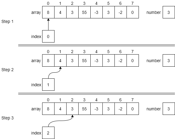
For linear search, we are simply iterating through the entire data structure until we find the desired item. So, while we can stop looking as soon as it is found, in the worst case we will have to look at all the elements in the structure, meaning the algorithm runs in order $N$ time.
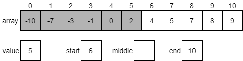
Binary search, on the other hand, takes advantage of a sorted array to jump around quickly. In effect, each element we analyze allows us to eliminate half of the remaining elements in our search. With as few as 8 steps, we can search through an array that contains 64 elements. When we analyze this algorithm, we find that it runs in order $\text{lg}(N)$ time, which is a vast improvement over binary search.
Of course, this only works when we can directly access elements in the middle of our data structure. So, while a linked list gives us several performance improvements over an array, we cannot use binary search effectively on a linked list.
In terms of memory usage, since both linear search and binary search just rely on the original data structures for storing the data, the extra memory usage is constant and consists of just a couple of extra variables, regardless of how many elements are in the data structure.
We have already discussed how much of an improvement binary search is over a linear search. In fact, our analysis showed that performing as few as 7 or 8 linear searches will take more time than sorting the array and using binary search. Therefore, in many cases we may want to sort our data. There are several different algorithms we can use to sort our data, but in this course we explored four of them: selection sort, bubble sort, merge sort, and quicksort.
The selection sort algorithm involves finding the smallest or largest value in an array, then moving that value to the appropriate end, and repeating the process until the entire array is sorted. Each time we iterate through the array, we look at every remaining element. In the module on sorting, we showed (through some clever mathematical analysis) that this algorithm runs in the order of $N^2$ time.
Bubble sort is similar, but instead of finding the smallest or largest element in each iteration, it focuses on just swapping elements that are out of order, and eventually (through repeated iterations) sorting the entire array. While doing so, the largest or smallest elements appear to “bubble” to the appropriate end of the array, which gives the algorithm its name. Once again, because the bubble sort algorithm repeatedly iterates through the entire data structure, it also runs on the order of $N^2$ time.
Both selection sort and bubble sort are inefficient as sorting algorithms go, yet their main value is their simplicity. They are also very nice in that they do not require any additional memory usage to run. They are easy to implement and understand and make a good academic example when learning about algorithms. While they are not used often in practice, later in this module we will discuss a couple of situations where we may consider them useful.
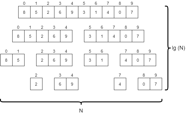
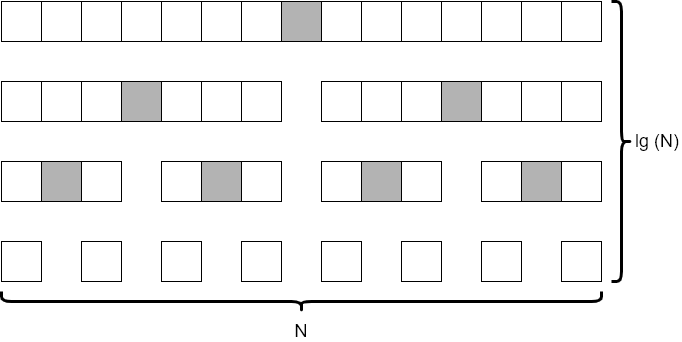
Merge sort is a very powerful divide and conquer algorithm, which splits the array to be sorted into progressively smaller parts until each one contains just one or two elements. Then, once those smaller parts are sorted, it slowly merges them back together until the entire array is sorted. We must look at each element in the array at least once per “level” of the algorithm in the diagram above, so overall this algorithm runs in the order of $N * \text{lg}(N)$ time. This is quite a bit faster than selection sort and bubble sort. However, most implementations of merge sort require at least a second array for storing data as it is merged together, so the additional memory usage is also on the order of $N$.
Quicksort is a very clever algorithm, which involves selecting a “pivot” element from the data, and then dividing the data into two halves, one containing all elements less than the pivot, and another with all items greater than the pivot. Then, the process repeats on each half until the entire structure is sorted. In the ideal scenario, shown in the diagram above, quicksort runs on the order of $N * \text{lg}(N)$ time, similar to merge sort. However, this depends on the choice of the pivot element being close to the median element of the structure, which we cannot always guarantee. Thankfully, in practice, we can just choose a random element (such as the last element in the structure) and we’ll see performance that is close to the $N * \text{lg}(N)$ target.
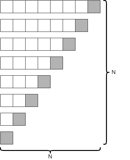
However, if we choose our pivot element poorly, the worst case scenario shown in the diagram above can occur, causing the run time to be on the order of $N^2$ instead. This means that quicksort has a troublesome, but rare, worst case performance scenario.
There are many different algorithms we can use to sort our data, and some of them can be shown mathematically to be more efficient, even in the worst case. So, how should we choose which algorithm to use?
In practice, it really comes down to a variety of factors, based on the amount of data we expect our program to handle, the randomness of the data, and more. The only way to truly know which algorithm is the best is to empirically test all of them and choose the fastest one, but even that approach relies on us predicting the data that our program will be utilizing.
Instead, here are some general guidelines we can use to help us select a sorting algorithm to use in our program.
Of course, the choice of which sorting algorithm to use is one of the most important decisions a programmer can make, and it is a great example of the fact that there are multiple ways to write a program that performs a particular task. Each possible program comes with various performance and memory considerations, and in many cases, there may not be a correct option. Instead, we must rely on our own knowledge and insight to choose the method that we feel would work best in any given situation.
Throughout this course, we have looked at a few ways we can use the data structures we have already learned to do something useful. In this module, we will look at a few of those examples again, as well as a few more interesting uses of the data structures that we have built.
First and foremost, it is important to understand that we can implement many of the simpler data structures such as stacks, queues and sets using both arrays and linked lists. In fact, from a certain point of view, there are only two commonly used containers for data – the array and the linked list. Nearly all other data structures are a variant of one of those two approaches or a combination of both.
Earlier in this chapter, we discussed some of the performance implications that arise when using arrays or linked lists to implement stacks and queues. In practice, we need to understand how we will be using our data in order to choose between the two approaches.
One unique use of sets appears in the code of compilers and interpreters. In each case, a programming language can only have one instance of a variable with a given name at any one time. So, we can think of the variables in a program as a set. In the code for a compiler or interpreter, we might find many instances of sets that are used to enforce rules that require each variable or function name to be unique.
Of course, this same property becomes important in even larger data storage structures, such as a relational database. For example, a database may include a column for a username or identification number which must be unique, such that no two entries can be the same. Once again, we can use a set to help enforce that restriction.
Hash tables are a great example of a data structure that effectively combines arrays and linked lists to increase performance. The best way to understand this is through the analysis of a set implemented using a hash table instead of a linked list.
When we determine if an element is already contained in a set based on a linked list, we must perform a linear search which runs on the order of $N$ time. The same operation performed on a set based on a hash table runs in constant time in the best case. This is because we can use the result of the hash function to jump directly to the bucket where the item should be stored, if it exists.
This same trick is used in large relational databases. If we have a database with a million rows, we can define an index for a column that allows us to quickly jump to entries without searching the entire database. To look up a particular entry using an index, we can calculate its hash, find the entry in the index, and then use the link in that index element to find the record in the database.
Finally, we can also use hash tables to build efficient indexes for large amounts of text data. Consider a textbook, for example. Most textbooks contain an index in the back that gives the page locations where particular terms are discussed. How can we create that index? We can iterate through each word in the textbook, but for each one we will have to search through the existing words in the index to see if that page is already listed for that word. That can be very slow if we must use a linear search through a linked list. However, if we use a hash table to store the index, the process of updating entries can be done in nearly constant time!
This page is the main page for Java Libraries
Both Java and Python include standard implementations of each of the data structures we have learned about in this course. While it is very useful and interesting from an academic perspective to build our own linked lists and hash tables, in practice we would rarely do so. In this section, we will briefly introduce the standard library versions of each data structure and provide references to where we can find more information about each one and how to use them.
In Java, most common data structures are part of the Java Collections Framework. It includes interfaces, implementations, and a variety of algorithms that can be used to do almost any common operation with data structures. You can find more information on the Java Tutorials website.
The most useful Java collection is the ArrayList . It performs very similarly to an array in most ways. Accessing an element in an ArrayList with an index runs in constant time, and adding new elements to the end of the container can also be done very quickly. In fact, most commonly used list operations run in constant time, and the memory and performance overhead that comes with using an ArrayList is very small.
ArrayLists in Java also support Generics
, which is a fancy way of saying that we can define the data types our collection should store and return, instead of just using Objects like we did in this course. We place this in angled brackets <> when we declare and instantiate the structure. This helps make our code easier to understand and can make it much easier to detect and correct type errors when we accidentally try to store an incorrect type in an ArrayList.
import java.util.ArrayList;

public class AList{
	public static void main(String[] args){
        ArrayList<Integer> alist = new ArrayList<Integer>();
        alist.add(1);
        alist.add(2);
        System.out.println(alist.get(0) + alist.get(1));
	}
}Java also includes an implementation of a LinkedList data structure. This structure also performs very similarly to the one we built in this class. Inserting or removing elements from the beginning and the end are constant time, as well as removing items from the middle of the list, provided we are using an iterator to find them.
LinkedLists in Java are also the ideal choice for implementing both Stacks and Queues because of the constant time operations for inserting and removing elements from the beginning and end of the list. In fact, it even includes the push(), pop() and peek() methods to simulate a stack, and uses offer() and poll() in place of enqueue() and dequeue() for queues.
LinkedLists in Java also support Generics . According to the Java documentation, when faced with a choice between ArrayList and LinkedList implementations of a particular container, in most cases the ArrayList implementation may be more performant. The exception would be when working with stacks and queues, in which case a LinkedList may work a bit better. When in doubt, they suggest trying the program with both structures and seeing which one performs better.
import java.util.LinkedList;

public class LList{
	public static void main(String[] args){
        LinkedList<Integer> llist = new LinkedList<Integer>();

        //Stack
        llist.push(new Integer(1));
        llist.push(new Integer(2));
        System.out.println(llist.peek());
        llist.pop();
        System.out.println(llist.pop());

        //Queue
        llist.offer(new Integer(1));
        llist.offer (new Integer(2));
        System.out.println(llist.peek());
        llist.poll();
        System.out.println(llist.poll());
    }
}Java includes three different implementations of the generic Map data structure, which stores a key-value pair. Two of them offer the ability to sort the keys or keep track of the order that elements were added to the structure, but we won’t review those here. The fastest is the HashMap , which doesn’t guarantee anything about the ordering of the keys or values but will give the best performance overall.
HashMaps in Java once again have support for Generics , which allows us to define the data type for both the keys and the values stored in the HashMap. This also simplifies things since we do not have to manage the creation of tuples outside of the collection. Instead, it is all handled internally.
import java.util.HashMap;

public class HMap{
	public static void main(String[] args){
        HashMap<String, Integer> hmap = new HashMap<String, Integer>();
        hmap.put(“Test”, new Integer(123));
        hmap.put(“Name”, new Integer(321));
        System.out.println(hmap.get(“Test”));
        hmap.remove(“Name”);
        System.out.println(hmap.containsKey(“Name”));
    }
}Java also includes a very fast implementation of the Set data structure called HashSet . It uses hashing to guarantee that each element is unique, and does not guarantee any particular ordering of the elements in the set. In fact, behind the scenes, the HashSet data structure uses a HashMap to store the data!
Unfortunately, the Set data structures in Java do not include straightforward implementations of many of the set operations, such as union, intersection, and subset. However, we can use a few of the included methods such as retainAll() and removeAll() to simulate those operations.
As with all the other Java data structures, HashSets also supports Generics , so we can define the data type it should be storing when we create it.
import java.util.HashSet;

public class HSet{
	public static void main(String[] args){
        HashSet<String> hset = new HashSet<String>();
        hset.add(“Test);
        hset.add(“Name”);
        System.out.println(hset.contains(“Name”));
        hset.remove(“Name”);
        System.out.println(hset.containsKey(“Name”));
    }
}Finally, we should also review the Java Collections class. It contains many static methods that we can use to work with the various collections we discussed above. For example, the Collections class includes methods for sorting a collection, finding the minimum or maximum value, determining if two collections are disjoint, and more.
Many of them are described in detail on the Algorithms page of the Collections tutorial.
Java also includes a special Arrays class that contains methods for manipulating raw arrays in a similar way.
Both of these classes are very useful to work with, since they help us avoid “reinventing the wheel” when we want to perform many common operations with our data.
This page is the main page for Python Libraries
Both Java and Python include standard implementations of each of the data structures we have learned about in this course. While it is very useful and interesting from an academic perspective to build our own linked lists and hash tables, in practice we would rarely do so. In this section, we will briefly introduce the standard library versions of each data structure and provide references to where we can find more information about each one and how to use them.
Python includes many useful data structures as built-in data types. We can use them to build just about any structure we need quickly and efficiently. The Python Tutorial has some great information about data structures in Python and how we can use them.
Python includes several data types that are grouped under the heading of sequence data types , and they all share many operations in common. We’ll look at two of the sequence data types: tuples and lists.
While we have not directly discussed tuples often, it is important to know that Python natively supports tuples as a basic data type. In Python, a tuple is simply a combination of a number of values separated by commas. They are commonly placed within parentheses, but it is not required.
We can directly access elements in a tuple using the same notation we use for arrays, and we can even unpack tuples into multiple variables or return them from functions. Tuples are a great way to pass multiple values as a single variable.
tuple1 = ‘a', ‘b', ‘c'
print(tuple1)  # (‘a', ‘b', ‘c')

tuple2 = (1, 2, 3, 4)
print(tuple2)  # (1, 2, 3, 4)
print(tuple2[0]) # 1
a, b, c, d = tuple2
print(d) # 4Python’s default data structure for sequences of data is the list . In fact, throughout this course, we have been using Python lists as a stand-in for the arrays that are supported by most other languages. Thankfully, lists in Python are much more flexible, since they can be dynamically resized, sliced, and iterated very easily. In terms of performance, a Python list is roughly equivalent to an array in other languages. We can access elements in constant time when the index is known, but inserting and removing from the beginning of the list runs in order of $N$ time since elements must be shifted backwards. This makes them a poor choice for queues and stacks, where elements must be added and removed from both ends of the list.
list1 = [‘a', ‘b', ‘c']
print(list1) # [‘a', ‘b', ‘c']
print(list1[1:2]) # [‘b', ‘c']The Python Collections library contains a special class called a deque (pronounced “deck”, and short for “double ended queue”) that is a linked list-style implementation that provides much faster constant time inserts and removals from either end of the container. In Python, it is recommended to use the deque data structure when implementing stacks and queues.
In a deque, the ends are referred to as “right” and “left”, so there are methods append() and pop() that impact the right side of the container, and appendleft() and popleft() that modify the left side. We can use a combination of those methods to implement both a Stack and a Queue using a deque in Python.
from collections import deque

# Stack
stack = deque()
stack.append(1)
stack.append(2)
print(stack[-1]) # 2 (peek right side)
print(stack.pop()) # 2
print(stack.pop()) # 1

# Queue
queue = deque()
queue.append(1)
queue.append(2)
print(queue[0]) # 1 (peek left side)
print(queue.popleft()) # 1
print(queue.popleft()) # 2Python also implements a version of the class Map data structure, called a dictionary . In Python, a dictionary stores key-value pairs, very similarly to how associative arrays work in other languages. Behind the scenes, it uses a hashing function to efficiently store and retrieve elements, making most operations run in near constant time.
The one limitation with Python dictionaries is that only hashable data types can be used as keys. We cannot use a list or a dictionary as the key for a dictionary in Python. Thankfully, strings, numbers, and most objects that implement a __hash__() and __eq__() method can be used.
dict = {‘name': 123, ‘test': 321}
print(dict[‘name']) # 123 (get a value)
dict[‘date'] = 456 # (add a new entry)
print(‘name' in dict) # True (search for entry)Python also includes a built in data type to represent a set . Just like we saw with our analysis, Python also uses a hash-based implementation to allow us to quickly find elements in the set, and therefore does not keep track of any ordering between the elements. We can easily add or remove elements, and Python uniquely allows us to use the binary operators to compute several set operations such as union and intersection.
set1 = {1, 3, 5, 7, 9}
set2 = {2, 3, 5, 7}
print(2 in set1) # False (check for membership)
print(2 in set2) # True (check for membership)

print(set1 – set2) # {1, 9} (set difference)
print(set1 | set2) # {1, 3, 5, 7, 9, 2} (union)
print(set1 & set2) # {3, 5, 7} (intersection)In this module, we reviewed each of the data structures we have explored in this class. Most importantly, we looked at how they compare in terms of performance and discussed some of the best and most efficient ways to use them in our programs.
Using that information, we introduced the standard collection libraries for both Java and Python, and saw how those professional implementations closely follow the same ideas and analysis that we saw in our own structures. While the professional structures may have many more features and more complex code, at the core they still work just like the structures we learned how to build from scratch.
One of the best traits of a good programmer is knowing how to most effectively use the tools made available to us through the programming languages and libraries we have chosen to use. The goal of this class is to give us the background we need to understand how the various collection data structures we can choose from work, so that we can use them in the most effective way to build useful and efficient programs.