Introducing Recursion

YouTube Video

We are now used to using functions in our programs that allow us to decompose complex problems into smaller problems that are easier to solve. Now, we will look at a slight wrinkle in how we use functions. Instead of simply having functions call other functions, we now allow for the fact that a function can actually call itself! When a function calls itself, we call it recursion.

Using recursion often allows us to solve complex problems elegantly—with only a few lines of code. Recursion is an alternative to using loops and, theoretically, any function that can be solved with loops can be solved with recursion and vice versa.

Example: Palindromes

So why would a function want to call itself? When we use recursive functions, we are typically trying to break the problem down into smaller versions of itself. For example, suppose we want to check to see if a word is a palindrome (i.e., it is spelled the same way forwards and backwards). How would we do this recursively? Typically, we would check to see if the first and last characters were the same. If so, we would check the rest of the word between the first and last characters. We would do this over and over until we got down to the 0 or 1 characters in the middle of the word. Let’s look at what this might look like in pseudocode.

function isPalindrome (String S) returns Boolean
    if length of S < 2 then
        return true
    else
        return (first character in S == last character in S) and 
                isPalindrome(substring of S without first and last character)
    end if
end function

First, we’ll look at the else part of the if statement. Essentially, this statement determines if the first and last characters of S match, and then calls itself recursively to check the rest of the word S. Of course, if the first and last characters of S match and the rest of the string is a palindrome, the function will return true. However, we can’t keep calling isPalindrome recursively forever. At some point we have to stop. That is what the if part of the statement does. We call this our base case. When we get to the point where the length of the string we are checking is 0 or 1 (i.e., < 2), we know we have reached the middle of the word. Since all strings of length 0 or 1 are, by definition, palindromes, we return true.

Key Idea: Break Up the Problem

The key idea of recursion is to break the problem into simpler subproblems until you get to the point where the solution to the problem is trivial and can be solved directly; this is the base case. The algorithm design technique is a form of divide-and-conquer called decrease-and-conquer. In decrease-and-conquer, we reduce our problem into smaller versions of the larger problem.

A recursive program is broken into two parts:

• a base case—a simple version of the problem that can be solved directly, and
• a recursive case—a general solution to the problem that uses smaller versions of the problem to compute the solution to the larger problem.

The base case is generally the final case we consider in a recursive function and serves to both end the recursive calls and to start the process of returning the final answer to our problem. To avoid endless cycles of recursive calls, it is imperative that we check to ensure that:

1. a base case exists where no further recursive calls are made, and
2. it is possible to reach the base case; the recursive case must ensure that we are moving closer to the base case with each recursive call.

Example: Reversing a String

Suppose we must write a program that reads in a sequence of keyboard characters and prints them in reverse order. The user ends the sequence by typing an asterisk character *.

We could solve this problem using an array, but since we do not know how many characters might be entered before the *, we could not be sure the program would actually work. However, we can use a recursive function since its ability to save the input data is not limited by a predefined array size.

Our solution would look something like this. We’ve also numbered the lines to make the following discussion easier to understand.

function REVERSE()			    (1)
    read CHARACTER			    (2)
    if CHARACTER == `*` then	(3)
        return			        (4)
    else				        (5)
        REVERSE()			    (6)
        print CHARACTER		    (7)
        return			        (8)
    end if 				        (9)
end function				    (10)

Base Case

The function first reads a single character from the keyboard and stores it in CHARACTER. Then, in line 3 it checks to see if the user typed the * character. If so, we simply return, knowing that we have reached the end of the input and need to start printing out the characters we’ve read in reverse order. This is the base case for this recursive function.

Recursive Case

If the CHARACTER we read in was not an *, line 6 will recursively call REVERSE to continue reading characters. Once the function returns (meaning that we have gotten an * character and started the return process) the function prints the CHARACTER in line 7 and then returns itself.

Behind the Scenes

Now let’s look at what happens within the computer when we run REVERSE. Let’s say the program user wants to enter the three characters from the keyboard: n, o, and w followed by the * character. The following figure illustrates the basic concept of what is going on in the computer.

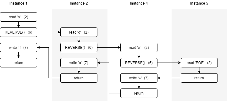
The arrows in the figure represent the order of execution of the statements in the computer. Each time we execute the recursive call to REVERSE in line 6, we create a new instance of the function, which starts its execution back at the beginning of the function (line 2). Then, when the function executes return, control reverts back to the next statement to be executed (line 7) in the calling instance of the function.

It’s important to understand that each instance of the function has its own set of variables whose values are unique to that instance. When we read n into the CHARACTER variable in the first instance of REVERSE it is not affected by anything that happens in the second instance of REVERSE. Therefore, reading the o into CHARACTER in the second instance of REVERSE does not affect the value of CHARACTER in the first instance of REVERSE.

During the execution of the first instance of REVERSE, the user enters the character n so the if condition is false and we execute the else part of the statement, which calls the REVERSE function. (Note that before we actually start the second instance of REVERSE, the operating system stores the statement where we will pick up execution once the called function returns.) When the second instance of REVERSE is started, a new copy of all variables is created as well to ensure we do not overwrite the values from the first instance.

The execution of the second instance of REVERSE runs exactly like the first instance except that the user enters the character o instead of n. Again, the else part of the if statement is executed, which calls the REVERSE function. When the third instance of REVERSE is executed, the user now inputs w, which again causes a new instance of REVERSE to be called.

Finally, in the fourth instance of REVERSE, the user inputs the * character, which causes the if part of the statement to execute, which performs our return statement. Once the return from the base case of our recursive function is performed, it starts the process of ending all the instances of the REVERSE function and creating the solution. When instance 4 of the REVERSE function returns, execution starts at the write statement (line 7) of instance 3. Here the character w is printed, and the function returns to instance 2. The same process is carried out in instance 2, which prints the o character and returns. Likewise, instance 1 prints its character n and then returns. The screen should now show the full output of the original call to REVERSE , which is “won”.

Recursion has allowed us to create a very simple and elegant solution to the problem of reversing an arbitrary number of characters. While you can do this in a non-recursive way using loops, the solution is not that simple. If you don’t believe us, just try it! (Yes, that is a challenge.)

Implementing Recursion

YouTube Video

function REVERSE2()			    (1)
    read CHARACTER			    (2)
    if CHARACTER == `*` then	(3)
        return			        (4)
    else				        (5)
        print CHARACTER		    (6a)
        REVERSE2()			    (7a)
        return			        (8)
    end if 				        (9)
end function				    (10)

The REVERSE2 function in the previous quiz actually prints the characters entered by the user in the same order in which they are typed. Notice how this small variation in the instruction order significantly changed the outcome of the function. To get a better understanding of why this occurs, we will delve into the order of execution in a little more depth.

Head and Tail Recursion

From the output of our original REVERSE function, we could argue that recursive function calls are carried out in a LIFO (last in, first out) order. Conversely, the output of the second version of the function REVERSE2, would lead us to believe that recursive function calls are carried out in FIFO (first in, first out) order. However, the ordering of the output is really based on how we structure our code within the recursive function itself, not the order of execution of the recursive functions.

To produce a LIFO ordering, we use a method called head recursion, which causes the function to make a recursive call first, then calculates the results once the recursive call returns. To produce a FIFO ordering, we use a method called tail recursion, which is when the function makes all of its necessary calculations before making a recursive call. With the REVERSE and REVERSE2 functions, this is simply a matter of swapping lines 6 and 7.

While some functions require the use of either head or tail recursion, many times we have the choice of which one to use. The choice is not necessarily just a matter of style, as we shall see next.

Tracing Program Execution

Before we finish our discussion of head and tail recursion, we need to make sure we understand how a recursive function actually works in the computer. To do this, we will use a new example. Let’s assume we want to print all numbers from 0 to $N$, where $N$ is provided as a parameter. A recursive solution to this problem is shown below.

function OUTPUT(integer N)			        (1)
    if N == 0 then					        (2)
        print N					            (3)
    else						            (4)
        print "Calling to OUTPUT " N-1		(5)
        OUTPUT(N-1)					        (6)
        print "Returning from OUTPUT " N-1	(7)
        print N					            (8)
    end if 						            (9)
    return						            (10)
end function							    (11)

Notice that we have added some extra print statements (lines 5 and 7) to the function just to help us keep track of when we have called OUTPUT and when that call has returned. This function is very similar to the REVERSE function above, we just don’t have to worry about reading a character each time the function runs. Now, if we call OUTPUT with an initial parameter of 3, we get the following output. We’ve also marked these lines with letters to make the following discussion simpler.

Calling to OUTPUT 2			(a)
Calling to OUTPUT 1			(b)
Calling to OUTPUT 0			(c)
0					        (d)
Returning from OUTPUT 0		(e)
1					        (f)
Returning from OUTPUT 1		(g)
2					        (h)
Returning from OUTPUT 2		(i)
3					        (j)

Lines a, b, and c show how the function makes all the recursive calls before any output or computation is performed. Thus, this is an example of head recursion which produces a LIFO ordering.

Once we get to the call of OUTPUT(0), the function prints out 0 (line d) and we start the return process. When we return from the call to OUTPUT(0) we immediately print out N, which is 1 and return. We continue this return process from lines g through j and eventually return from the original call to OUTPUT having completed the task.

Looking Under the Covers

Now that we have seen how recursion works in practice, we will pull back the covers and take a quick look at what is going on underneath. To be able to call the same function over and over, we need to be able to store the appropriate data related to each function call to ensure we can treat it as a unique instance of the function. While we do not make copies of the code, we do need to make copies of other data. Specifically, when function A calls function B, we must save the following information:

• the memory address of the current parameters,
• the address of the statement in function A to be executed when B returns (called the return address),
• the address of the memory location that will contain the value returned by the function (the value address), and
• all the local variables of function B.

We call this information the activation record for function A. When a call to B is made, this information is stored in a stack data structure known as the activation stack, and execution begins at the first instruction in function B. Upon completion of function B, the following steps are performed.

1. The return address is read from the activation stack.
2. The information stored about function B is removed from the activation stack, leaving the information stored for function A on top of the stack.
3. Execution begins at the return address in function A.

Next, we will look at how we use the activation stack to implement recursion. For this we will use a simple MAIN program that calls our simplified OUTPUT function (where we have removed all the print statements used to track our progress).

function MAIN()
    OUTPUT(3) 					(1)
    print ("Done")				(2)
end function

function OUTPUT(integer N)
    if N == 0 then				(1)
        print N					(2)
    else						(3)
        OUTPUT(N-1)				(4)
        print N					(5)
    end if 						(6)
    return						(7)
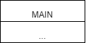
end function

When we run MAIN, the only record on the activation stack is the record for MAIN. Since it has not been “called” from another function, it does not contain a return address. It also has no local variables, so the record is basically empty as shown below.

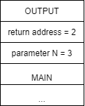
However, when we execute line 1 in MAIN, we call the function OUTPUT with a parameter of 3. This causes the creation of a new function activation record with the return address of line 3 in the calling MAIN function and a parameter for N, which is 3. Again, there are no local variables in OUTPUT. The stack activation is shown in figure a below.

a	b	c	d

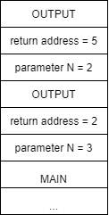
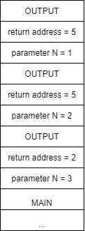
Following the execution for OUTPUT, we will eventually make our recursive call to OUTPUT in line 4, which creates a new activation record on the stack as shown above in b. This time, the return address will be line 5 and the parameter N is 2.

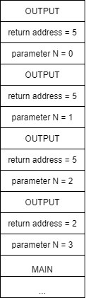
Execution of the second instance of OUTPUT will follow the first instance, eventually resulting in another recursive call to OUTPUT and a new activation record as shown in c above. Here the return address is again 5 but now the value of parameter N is 1. Execution of the third instance of OUTPUT yields similar results, giving us another activation record on the stack d with the value of parameter N being 0.

Finally, the execution of the fourth instance of OUTPUT will reach our base case of N == 0. Here we will write 0 in line 2 and then return. This return will cause us to start execution back in the third instance of OUTPUT at the line indicated by the return value, or in this case, 5. The stack activation will now look like e in the figure below.

e	f	g	h

When execution begins in the third instance of OUTPUT at line 5, we again write the current value of N, which is 1, and we then return. We follow this same process, returning to the second instance of OUTPUT, then the first instance of OUTPUT. Once the initial instance of OUTPUT completes, it returns to line 2 in MAIN, where the print("Done") statement is executed and MAIN ends.

Performance

While recursion is a very powerful technique, its expressive power has an associated cost in terms of both time and space. Anytime we call a function, a certain amount of memory space is needed to store information on the activation stack. In addition, the process of calling a function takes extra time since we must store parameter values and the return address, etc. before restarting execution. In the general case, a recursive function will take more time and more memory than a similar function computed using loops.

Recursion Versus Iteration

It is possible to demonstrate that any function with a recursive structure can be transformed into an iterative function that uses loops and vice versa. It is also important to know how to use both mechanisms because there are advantages and disadvantages for both iterative and recursive solutions. While we’ve discussed the fact that loops are typically faster and take less memory than similar recursive solutions, it is also true that recursive solutions are generally more elegant and easier to understand. Recursive functions can also allow us to find solutions to problems that are complex to write using loops.

Example: Factorials

The most popular example of using recursion is calculating the factorial of a positive integer $N$. The factorial of a positive integer $N$ is just the product of all the integers from $1$ to $N$. For example, the factorial of $5$, written as $5!$, is calculated as $5 * 4 * 3 * 2 * 1 = 120$. The definition of the factorial function itself is recursive. $$ \text{fact}(N) = N * \text{fact}(N - 1) $$ The corresponding pseudocode is shown below.

function FACT(N)
    if N == 1
        return 1
    else
        return N * FACT(N-1)
    end if
end function

The recursive version of the factorial is slower than the iterative version, especially for high values of $N$. However, the recursive version is simpler to program and more elegant, which typically results in programs that are easier to maintain over their lifetimes.

Tree Recursion

YouTube Video

In the previous examples we saw recursive functions that call themselves one time within the code. This type of recursion is called linear recursion, where head and tail recursion are two specific types of linear recursion.

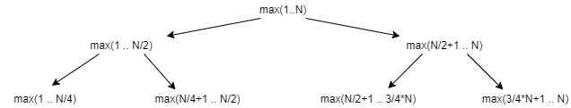
In this section we will investigate another type of recursion called tree recursion, which occurs when a function calls itself two or more times to solve a single problem. To illustrate tree recursion, we will use a simple recursive function MAX, which finds the maximum of $N$ elements in an array. To calculate the maximum of $N$ elements we will use the following recursive algorithm.

1. Compute the maximum of the first $N/2$ elements and store in MAX1.
2. Compute the maximum of the last $N/2$ elements and store in MAX2.
3. Compare MAX1 and MAX2 to find the maximum of all elements.

Our process recursively decomposes the problem by searching for the maximum in the first $N/2$ elements and the second $N/2$ elements until we reach the base case. In this problem, the base case is when we either have 1 or 2 elements in the array. If we just have 1, we return that value. If we have 2, we return the larger of those two values. An overview of the process is shown below.

The pseudocode for the algorithm is shown below.

function MAX(VALUES, START, END)
    print "Called MAX with start = " + START + ", end = " + END
    if END – START = 0
        return VALUES[START]
    else if END – START = 1
        if VALUES(START) > VALUES(END)
            return VALUES[START]
        else
            return VALUES[END]
        end if
    else
        MIDDLE = ROUND((END – START) / 2) 
        MAX1 = MAX(VALUES, START, START + MIDDLE – 1)
        MAX2 = MAX(VALUES, START + MIDDLE, END)
        if MAX1 > MAX2
            return MAX1
        else
            return MAX2
        end if
    end if
end function

The following block shows the output from the print line in the MAX function above. The initial call to the function is MAX(VALUES, 0, 15).

Called MAX with start = 0, end = 7
Called MAX with start = 0, end = 3
Called MAX with start = 0, end = 1
Called MAX with start = 2, end = 3
Called MAX with start = 4, end = 7
Called MAX with start = 4, end = 5
Called MAX with start = 6, end = 7
Called MAX with start = 8, end = 15
Called MAX with start = 8, end = 11
Called MAX with start = 8, end = 9
Called MAX with start = 10, end = 11
Called MAX with start = 12, end = 15
Called MAX with start = 12, end = 13
Called MAX with start = 14, end = 15

As you can see, MAX decomposes the array each time it is called, resulting in 14 instances of the MAX function being called. If we had performed head or tail recursion to compare each value in the array, we would have to have called MAX 16 times. While this may not seem like a huge savings, as the value of $N$ grows, so do the savings.

Example: Fibonacci Numbers

YouTube Video

Next, we will look at calculating Fibonacci numbers using a tree recursive algorithm. Fibonacci numbers are given by the following recursive formula. $$ f_n = f_{n-1} + f_{n-2} $$ Notice that Fibonacci numbers are defined recursively, so they should be a perfect application of tree recursion! However, there are cases where recursive functions are too inefficient compared to an iterative version to be of practical use. This typically happens when the recursive solutions to a problem end up solving the same subproblems multiple times. Fibonacci numbers are a great example of this phenomenon.

Calculating Fibonacci Numbers

To complete the definition, we need to specify the base case, which includes two values for the first two Fibonacci numbers: FIB(0) = 0 and FIB(1) = 1. The first Fibonacci numbers are $0, 1, 1, 2, 3, 5, 8, 13, 21 …$.

Producing the code for finding Fibonacci numbers is very easy from its definition. The extremely simple and elegant solution to computing Fibonacci numbers recursively is shown below.

function FIB(N)
    if N == 0
        return 0
    else if N == 1
        return 1
    else
        return FIB(N-1) + FIB(N-2)
    end if
end function

The following pseudocode performs the same calculations for the iterative version.

function FIBIT(N)
    FIB1 = 1
    FIB2 = 0
    for (I = 2 to N)
        FIB = FIB1 + FIB2
        FIB2 = FIB1
        FIB1 = FIB
    end loop
end function

While this function is not terribly difficult to understand, there is still quite a bit of mental gymnastics required to see how this implements the computation of Fibonacci numbers and even more to prove that it does so correctly. However, as we will see later, the performance improvements of the iterative solution are worth it.

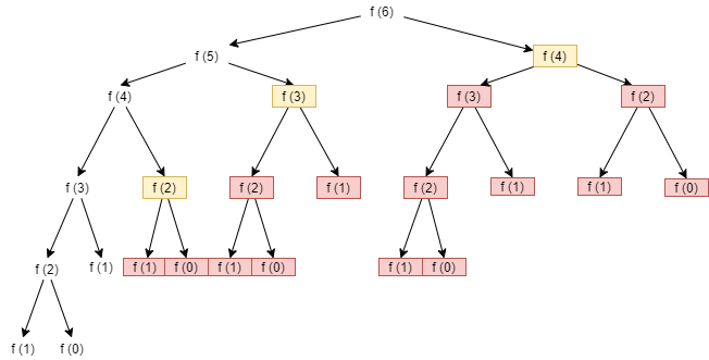
If we analyze the computation required for the 6th Fibonacci number in both the iterative and recursive algorithms, the truth becomes evident. The recursive algorithm calculates the 5th Fibonacci number by recursively calling FIB(4) and FIB(3). In turn, FIB(4) calls FIB(3) and FIB(2). Notice that FIB(3) is actually calculated twice! This is a problem. If we calculate the 36th Fibonacci number, the values of many Fibonacci numbers are calculated repeatedly, over and over.

Tracing the Program

To clarify our ideas further, we can consider the recursive tree resulting from the trace of the program to calculate the 6th Fibonacci number. Each of the computations highlighted in the diagram will have been computed previously.

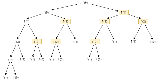
If we count the recomputations, we can see how we calculate the 4th Fibonacci number twice, the 3rd Fibonacci number three times, and the 2nd Fibonacci five times. All of this is due to the fact the we do not consider the work done by other recursive calls. Furthermore, the higher our initial number, the worse the situation grows, and at a very rapid pace.

Memoization

To avoid recomputing the same Fibonacci number multiple times, we can save the results of various calculations and reuse them directly instead of recomputing them. This technique is called memoization, which can be used to optimize some functions that use tree recursion.

To implement memoization, we simply store the values the first time we compute them in an array. The following pseudocode shows an efficient algorithm that uses an array, called FA, to store and reuse Fibonacci numbers.

function FIBOPT(N)
    if N == 0
        return 0
    else if N == 1
        return 1
    else if FA[N] == -1
        FA[N] = FIBOPT(N-1) + FIBOPT(N-2)
        return FA[N]
    else
        return FA[N]
    end if
end function

We assume that each element in FA has been initialized to -1. We also assume that N is greater than 0 and that the length of FA is larger than the Fibonacci number N that we are trying to compute. (Of course, we would normally put these assumptions in our precondition; however, since we are focusing on the recursive nature of the function, we will not explicitly show this for now.) The cases where N == 0 and N == 1 are the same as we saw in our previous FIB function. There is no need to store these values in the array when we can return them directly, since storing them in the array takes additional time. The interesting cases are the last two. First, we check to see if FA[N] == -1, which would indicate that we have not computed the Fibonacci number for N yet. If we have not yet computed N’s Fibonacci number, we recursively call FIBOPT(N-1) and FIBOPT(N-2) to compute its value and then store it in the array and return it. If, however, we have already computed the Fibonacci for N (i.e., if FA[N] is not equal to -1), then we simply return the value stored in the array, FA[N].

As shown in our original call tree below, using the FIBOPT function, none of the function calls in red will be made at all. While the function calls in yellow will be made, they will simply return a precomputed value from the FA array. Notice that for N = 6, we save 14 of the original 25 function calls required for the FIB function, or a $56%$ savings. As N increases, the savings grow even more.

Example: Tower of Hanoi

There are some problems where an iterative solution is difficult to implement and is not always immediately intuitive, while a recursive solution is simple, concise and easy to understand. A classic example is the problem of the Tower of Hanoi .

The Tower of Hanoi is a game that lends itself to a recursive solution. Suppose we have three towers on which we can put discs. The three towers are indicated by a letter, A, B, or C.

Now, suppose we have $N$ discs all of different sizes. The discs are stacked on tower A based on their size, smaller discs on top. The problem is to move all the discs from one tower to another by observing the following rules:

1. we can move only one disc at a time, and we must move the disc that is at the top of a tower first, and
2. a larger disc can never be put on top of a smaller disc.

To try to solve the problem let’s start by considering a simple case: we want to move two discs from tower A to tower C. As a convenience, suppose we number the discs in ascending order by assigning the number 1 to the larger disc. The solution in this case is simple and consists of the following steps:

1. move disc 2 from tower A to tower B,
2. move disc 1 from tower A to tower C, and
3. move disc 2 from Tower B to tower C.

The following figure shows how the algorithm works.

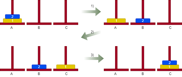
It is a little more difficult with three discs, but after a few tries the proper algorithm emerges. With our knowledge of recursion, we can come up with a simple and concise solution. Since we already know how to move two discs from one place to another, we can solve the problem recursively.

1. Move discs 3 and 2 from tower A to B.
2. Move disc 1 from tower A to C.
3. Move discs 3 and 2 from tower B to C.

In formulating our solution, we assumed that we could move two discs from one tower to another, since we have already solved that part of the problem above. In step 1, we use this solution to move the top two discs from tower A to B. Then, in step 3, we again use that solution to move two discs from tower B to C. This process can now easily be generalized to the case of N discs as described below.

1. Move the first N-1 discs from tower A to B.
2. Move disc 1 from tower A to C.
3. Move N -1 discs from tower B to C.

The algorithm is captured in the following pseudocode. Here N is the total number of discs, ORIGIN is the tower where the discs are currently located, and DESTINATION is the tower where they need to be moved. Finally, TEMP is a temporary tower we can use to help with the move. All the parameters are integers.

function HANOI(N, ORIGIN, DESTINATION, TEMP)
    if N >= 0
        HANOI(N-1, ORIGIN, TEMP, DESTINATION)
        Move disc N from ORIGIN to DESTINATION
        HANOI(N-1, TEMP, DESTINATION, ORIGIN)
    end if
    return
end function

The function moves the $N$ discs from the source tower to the destination tower using a temporary tower. To do this, it calls itself to move the first $N-1$ discs from the source tower to the temporary tower. It then moves the bottom disc from the source tower to the destination tower. The function then moves the $N-1$ discs present in the temporary tower into the destination tower.

The list of movements to solve the three-disc problem is shown below.

1. move disc 3 from ORIGIN to DESTINATION
2. move disc 2 from ORIGIN to TEMP
3. move disc 3 from DESTINATION to TEMP
4. move disc 1 from ORIGIN to DESTINATION
5. move disc 3 from TEMP to ORIGIN
6. move disc 2 from TEMP to DESTINATION

Iterative solutions to the Tower of Hanoi problem do exist, but it took many researchers several years to find an efficient solution. The simplicity of finding the recursive solution presented here should convince you that recursion is an approach you should definitely keep in your bag of tricks!

Converting Recursion to Iteration

Iteration and recursion have the same expressive power, which means that any problem that has a recursive solution also has an iterative solution and vice versa. There are also standard techniques that allow you to transform a recursive program into an equivalent iterative version. The simplest case is for tail recursion, where the recursive call is the last step in the function. There are two cases of tail recursion to consider when converting to an iterative version.

1. If the recursive function does not have any parameters or the parameters are passed by reference, the conversion is very simple. We just use a simple while loop.
2. If the recursive function uses parameters passed by value, the conversion is a little more complicated. In general, if the last statement a function f(x) executes is a call to itself, f(y) with parameter y, the recursive call can be replaced by an assignment statement, x = y, and by looping back to the beginning of function f.

The approach above only solves the conversion problem in the case of tail recursion. However, as an example, consider our original FACT function and its iterative version FACT2. Notice that in FACT2 we had to add a variable fact to keep track of the actual computation.

function FACT(N)
    if N == 1
        return 1
    else
        return N * FACT(N-1)
    end if
end function

function FACT2(N)
   fact = 1 
   while N > 0
       fact = fact * N
       N = N - 1
   end while
   return fact
end function

The conversion of non-tail recursive functions typically uses two loops to iterate through the process, effectively replacing recursive calls. The first loop executes statements before the original recursive call, while the second loop executes the statements after the original recursive call. The process also requires that we use a stack to save the parameter and local variable values each time through the loop. Within the first loop, all the statements that precede the recursive call are executed, and then, before the loop terminates, the values of interest are pushed onto the stack. The second loop starts by popping the values saved on the stack and then executing the remaining statements that come after the original recursive call. This is typically much more difficult than the conversion process for tail recursion.

Recursion Summary

In this module, we explored the use of recursion to write concise solutions for a variety of problems. Recursion allows us to call a function from within itself, using either head recursion, tail recursion or tree recursion to solve smaller instances of the original problem.

Recursion requires a base case, which tells our function when to stop calling itself and start returning values, and a recursive case to handle reducing the problem’s size and calling the function again, sometimes multiple times.

We can use recursion in many different ways, and any problem that can be solved iteratively can also be solved recursively. The power in recursion comes from its simplicity in code—some problems are much easier to solve recursively than iteratively.

Unfortunately, in general a recursive solution requires more computation time and memory than an iterative solution. We can use techniques such as memoization to greatly improve the time it takes for a recursive function to execute, especially in the case of calculating Fibonacci numbers where subproblems are overlapped.