Quicksort Time Complexity

To wrap up our analysis of the quicksort algorithm, let’s take a look at the time complexity of the algorithm. Quicksort is a very difficult algorithm to analyze, especially since the selection of the pivot value is random and can greatly affect the performance of the algorithm. So, we’ll talk about quicksort’s time complexity in terms of two cases, the worst case and the average case. Let’s look at the average case first

Average case complexity

What would the average case of quicksort look like? This is a difficult question to answer and requires a bit of intuition and making a few assumptions. The key really lies in how we choose our pivot value.

First, let’s assume that the data in our array is equally distributed. This means that the values are evenly spread between the lowest value and the highest value, with no large clusters of similar values anywhere. While this may not always be the case in the real world, often we can assume that our data is somewhat equally distributed.

Second, we can also assume that our chosen pivot value is close to the average value in the array. If the array is equally distributed and we choose a value at random, we have a $50%$ chance of that value being closer to the average than either the minimum or the maximum value, so this is a pretty safe assumption.

With those two assumptions in hand, we see that something interesting happens. If we choose the average value as our pivot value, quicksort will perfectly partition the array into two equal sized halves! This is a great result, because it means that each recursive call to the function will be working with data that is half the initial array.

If we consider an array that initially contains $15$ elements, and make sure that we always choose the average element as our pivot point, we’d end up with a tree of recursive calls that resembles the diagram below.

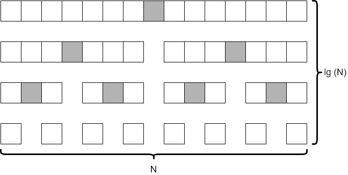
In this diagram, we see that each level of the tree looks at around $N$ elements. (It is actually fewer, but not by a significant amount so we can just round up to $N$ each time). We also notice that there are 4 levels to the tree, which is closely approximated by $\text{lg}(N)$. This is the same result we observed when analyzing the merge sort algorithm earlier in this module.

So, in the average case, we’d say that quicksort runs in the order of $N * \text{lg}(N)$ time.

Worst case complexity

To consider the worst-case situation for quicksort, we must come up with a way to define what the worst-case input would be. It turns out that the selection of our pivot value is the key here.

Consider the situation where the pivot value is chosen to be the maximum value in the array. What would happen in that case?

Looking at the code, we would see that each recursive call would contain one empty partition, and the other partition would be just one less than the size of the original array. So, if our original array only contained 8 elements, our tree recursion diagram would look similar to the following.

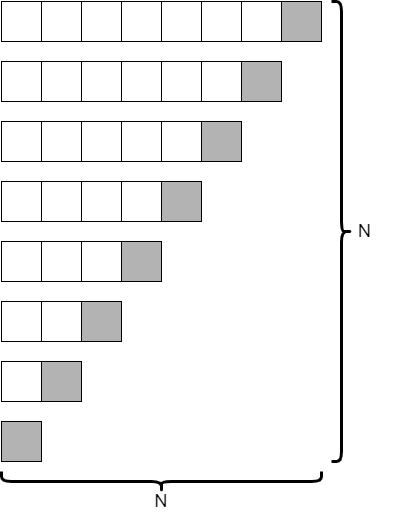
This is an entirely different result! In this case, since we are only reducing the size of our array by 1 at each level, it would take $N$ recursive calls to complete. However, at each level, we are looking at one fewer element. Is this better or worse than the average case?

It turns out that it is much worse. As we learned in our analysis of selection sort and bubble sort, the series

$$ N + (N – 1) + (N – 2) + … + 2 + 1 $$

is best approximated by $N^2$. So, we would say that quicksort runs in the order of $N^2$ time in the worst case. This is just as slow as selection sort and bubble sort! Why would we ever call it “quicksort” if it isn’t any faster?

Thankfully, in practice, it is very rare to run into this worst-case performance with quicksort, and in fact most research shows that quicksort is often the fastest of the four sorting algorithms we’ve discussed so far. In the next section, we’ll discuss these performance characteristics a bit more.

This result highlights why it is important to consider both the worst case and average case performance of our algorithms. Many times we’ll write an algorithm that runs well most of the time, but is susceptible to poor performance when given a particular worst-case input.