Welcome!
This page is the main page for Searching and Sorting
This page is the main page for Searching and Sorting
In this course, we are learning about many different ways we can store data in our programs, using arrays, queues, stacks, lists, maps, and more. We’ve already covered a few of these data structures, and we’ll learn about the others in upcoming modules. Before we get there, we should also look at a couple of the most important operations we can perform on those data structures.
Consider the classic example of a data structure containing information about students in a school. In the simplest case, we could use an array to store objects created from a Student class, each one representing a single student in the school.
As we’ve seen before, we can easily create those objects and store them in our array. We can even iterate through the array to find the maximum age or minimum GPA of all the students in our school. However, what if we want to just find a single student’s information? To do that, we’ll need to discuss one of the most commonly used data structure operations: searching.
Searching typically involves finding a piece of information, or a value stored in a data structure or calculated within a specific domain. For example, we might want to find out if a specific word is found in an array of character strings. We might also want to find an integer that meets a specific criterion, such as finding an integer that is the sum of the two preceding integers. For this module, we will focus on finding values in data structures.
In general, we can search for
The data structure can be thought of more generally as a container, which can be
For the examples in this module, we’ll generally use a simple finite array as our container. However, it shouldn’t be too difficult to figure out how to expand these examples to work with a larger variety of data structures. In fact, as we introduce more complex data structures in this course, we’ll keep revisiting the concept of searching and see how it applies to the new structure.
In general, containers can be either ordered or unordered. In many cases, we may also use the term sorted to refer to an ordered container, but technically an ordered container just enforces an ordering on values, but they may not be in a sorted order. As long as we understand what the ordering is, we can use that to our advantage, as we’ll see later.
Searches in an unordered container generally require a linear search, where every value in the container must be compared against our search value. On the other hand, search algorithms on ordered containers can take advantage of this ordering to make their searches more efficient. A good example of this is binary search. Let’s begin by looking at the simplest case, linear search.
When searching for a number in an unordered array, our search algorithms are typically designed as functions that take two parameters:
Our search functions then return an index to the number within the array.
In this module, we will develop a couple of examples of searching an array for a specific number.
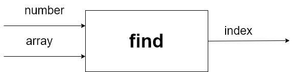
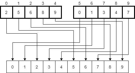
Finding the first occurrence of a number in an unordered array is a fairly straightforward process. A black box depiction of this function is shown below. There are two inputs–array and number–and a single output, the index of the first occurrence of the number in array.
We can also include the search function as a method inside of the container itself. In that case, we don’t have to accept the container as a parameter, since the method will know to refer to the object it is part of.
Of course, when we begin designing an algorithm for our function we should think about two items immediately: the preconditions and the postconditions of the function. For this function, they are fairly simple.
The precondition for find is that the number provided as input is compatible with the type of data held by the provided array. In this case, we have no real stipulations on array. It does not need to actually have any data in it, nor does it have to be ordered or unordered.
Our postcondition is also straightforward. The function should return the index of number if it exists in the array. However, if number is not found in the array, then -1 is returned. Depending on how we wish to implement this function, it could also return another default index or throw an exception if the desired value is not found. However, most searching algorithms follow the convention of returning an invalid index of -1 when the value is not found in the array, so that’s what we’ll use in our examples.
Preconditions:
Postconditions:
To search for a single number in our array, we will use a loop to search each location in the array until we find the number. The general idea is to iterate over all the elements in the array until we either find the number we are searching for or there are no other elements in the array.
function FIND(NUMBER, ARRAY)						(1)
    loop INDEX from 0 to size of ARRAY - 1 			(2)
        if ARRAY[INDEX] == NUMBER					(3)
            return INDEX							(4)
        end if								        (5)
    end for									        (6)
    return -1								        (7)
end function									    (8)
As we can see in line 1, the function takes both a number and array parameter. We then enter a for loop in line 2 to loop through each location in the array. We keep track of the current location in the array using the index variable. For each location, we compare number against the value in the array at location index. If we find the number, we simply return the value of index in line 4. If we do not find the number anywhere in the array, the loop will exit, and the function will return -1 in line 8.
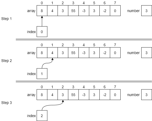
Below is an example of how to execute this algorithm on example data. Step 1 shows the initial state of the variables in the function the first time through the loop. Both array and number are passed to the function but we do not modify either of them in the function. The index variable is the for loop variable, which is initially set to 0 the first time through the loop. In line 3, the function compares the number in array[index] against the value of number. In this step, since index is 0, we use array[0], which is 8. Since 8 is not equal to the value of number, which is 3, we do nothing in the if statement and fall to the end for statement in line 6. Of course, this just sends us back to the for statement in line 2.
The second time through the for loop is shown as Step 2 in the figure. We follow the same logic as above and compare array[1], or 4, against number, which is still 3. Since these values are not equal, we skip the rest of the if statement and move on to Step 3.
In Step 3, index is incremented to 2, thus pointing at array[2], whose value is 3. Since this value is equal to the value of number, we carry out the if part of the statement. Line 4 returns the value of 2, which is the first location in array that holds the value of number.
Our find algorithm above will find the first instance of number in the array and return the index of that instance. However, we might also be interested in finding the last instance of number in array. Looking at our original find algorithm, it should be easy to find the last value by simply searching the array in reverse order, as shown in the following figure.
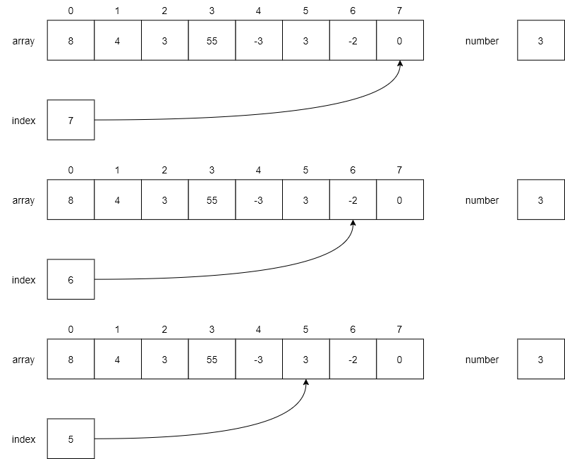
We will use the same example as above, except we will start searching backwards from the end of the array. In Step 1, we see that index is initialized to 7 and we compare array[7] against number, which are not the same. Thus, we continue to Step 2, where we decrement index to 6. Here array[6] is still not equal to number, so we continue in the loop. Finally, in Step 3, we decrement index to 5. Now array[5] contains the number 3, which is equal to our number and we return the current index value.
Luckily for us, we can change our for loop index to decrement from the end of the array (size of array - 1) to the beginning (0). Thus, by simply changing line 3 in our original function, we can create a new function that searches for the last instance of number in array. The new function is shown below.
function REVERSEFIND(NUMBER, ARRAY)					   (1)
    loop INDEX from size of ARRAY – 1 to 0 step -1	   (2)
        if ARRAY[INDEX] == NUMBER					   (3)
            return INDEX							   (4)
        end if								           (5)
    end for									           (6)
    return -1								           (7)
end function									       (8)
Obviously, the for loop in line 2 holds the key to searching our array in reverse order. We start at the end of the array by using the index size of array - 1 and then decrement the value of index (via the step -1 qualifier) each time through the loop until we reach 0. The remainder of the function works exactly like the find function.
We looked at an iterative version of the find function above. But what would it take to turn that function into a recursive function? While for this particular function, there is not a lot to be gained from the recursive version, it is still instructive to see how we would do it. We will find recursive functions more useful later on in the module.
In this case, to implement a recursive version of the function, we need to add a third parameter, index, to tell us where to check in the array. We assume that at the beginning of a search, index begins at 0. Then, if number is not in location index in the array, index will be incremented before making another recursive call. Of course, if number is in location index, we will return the number of index. The pseudocode for the findR function is shown below.
function FINDR (NUMBER, ARRAY, INDEX) 		       (1)
    if INDEX >= size of ARRAY then				   (2)
        return -1								   (3)
    else if ARRAY[INDEX] == NUMBER				   (4)
        return INDEX							   (5)
    else									       (6)
        return FINDR (NUMBER, ARRAY, INDEX + 1)	   (7)
    end if									       (8)
end function									   (9)
First, we check to see if index has moved beyond the bounds of the array, which would indicate that we have searched all the locations in array for number. If that is the case, then we return -1 in line 3 indicating that we did not find number in array. Next, we check to see if number is found in array[index] in line 4. If it is, the we are successful and return the index. However, if we are not finished searching and we have not found number, then we recursively call findR and increment index by 1 to search the next location.
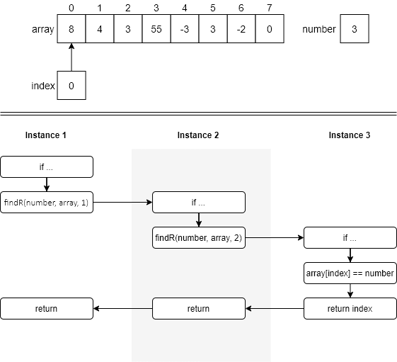
An example of using the findR function is shown below. The top half of the figure shows the state of the data in the initial call to the findR function (instance 1). The bottom half of the figure shows the recursive path through the function. The beginning of instance 1 shows the if statement in line 2. In instance 1, since we have not searched the entire array (line 2) and array[0] is not equal to number (line 4), we fall down to the else part function and execute line 7, the recursive call. Since index is 0 in instance 1, we call instance 2 of the function with an index of 1.
In instance 2, the same thing happens as in instance 1 and we fall down to the else part of the if statement. Once again, we call a new instance of findR, this time with index set at 2. Now, in instance 3, array[index] is equal to number in line 4 and so we execute the return index statement in line 5. The value of index (2) is returned to instance 2, which, in line 7, simply returns the value of 2 to instance 1. Again, in line 7, instance 1 returns that same value (2) to the original calling function.
Notice that the actual process of searching the array is the same for both the iterative and recursive functions. It is only the implementation of that process that is different between the two.
We may also want to search through a data structure to find an item with a specific property. For example, we could search for the student with the maximum age, or the minimum GPA. For this example, let’s consider the case where we’d like to find the minimum value in an array of integers.
Searching for the minimum number in an unordered array is a different problem than searching for a specific number. First of all, we do not know what number we are searching for. And, since the array is not ordered, we will have to check each and every number in the array.
The input parameters of our new function will be different from the find function above, since we do not have a number to search for. In this case, we only have an array of numbers as an input parameter. The output parameter, however, is the same. We still want to return the index of the minimum number in the array. In this case, we will return -1 if there is no minimum number, which can only happen if there is no data in the array when we begin.
Preconditions:
Postconditions:
Our preconditions and postconditions are also simple. Our precondition is simply that we have an array whose data can be sorted. This is important, because it means that we can compare two elements in the array and determine which one has a smaller value. Otherwise, we couldn’t determine the minimum value at all!
Our postcondition is that we return the minimum number of the data in the array, or -1 if the array is empty.
The function findMin is shown below. First, we check to see if the array is empty. If it is, we simply return -1 in line 3. If not, we assume the location 0 contains the minimum number in the array, and set min equal to 0 in line 5. Then we loop through each location in the array (starting with 1) in line 6 and set min equal to the minimum of the array data at the current index and the data at min. (Note: if the array only has a single number in it, the for loop will not actually execute since index will be initialized to 1, which is already larger than the size of the array – 1, which is 0.) Once we complete the loop, we will be guaranteed that we have the index of the minimum number in the array.
function FINDMIN(ARRAY) (1)
if ARRAY is empty then (2)
return -1 (3)
end if (4)
MIN = 0 (5)
loop INDEX from 1 to size of ARRAY - 1 (6)
if ARRAY[INDEX] < ARRAY[MIN] (7)
MIN = INDEX (8)
end if (9)
end for (10)
return MIN (11)
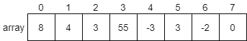
end function (12)Next, we will walk through the algorithm using our example array in the figure below. Step 1 shows the initial time through the loop. In line 5, min is set to 0 by default and in line 6, index is set equal to 1. Line 7 then computes whether array[1] < array[0]. In this case, it is and we set min = 1 (which is reflected in the next step where min has the value 1).
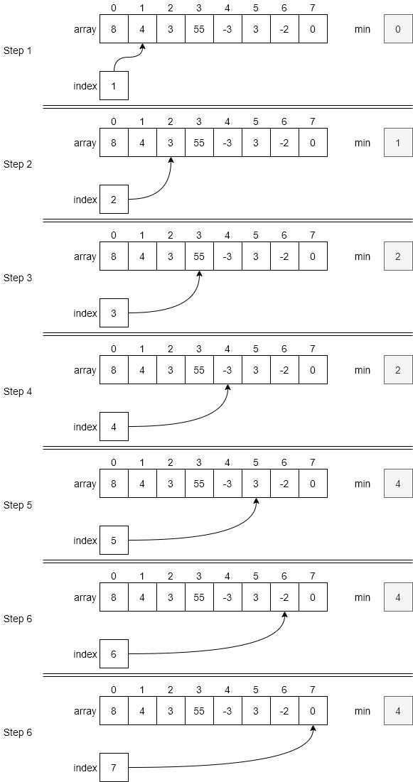
Step 2 will end up comparing array[2] < array[1], since min is now 1 and index has been incremented to 2 via the for loop. In this case, array[2] is less than array[1] so we update min again, this time to 2.
Step 3 follows the same process; however, this time the value in array[3] is 55, which is greater than the current minimum of 3 in array[2]. Therefore, min is not updated. Step 4 finds the minimum value in the array of -3 at index 4 and so updates min to 4. However, steps 5, 6, and 7 do not find new minimum values. Thus, when the loop exits after Step 6, min is set to 4 and this value is returned to the calling program in line 11.
We’ve examined many different versions of a linear search algorithm. We can find the first occurrence of a number in an array, the last occurrence of that number, or a value with a particular property, such as the minimum value. Each of these are examples of a linear search, since we look at each element in the container sequentially until we find what we are looking for.
So, what would be the time complexity of this process? To understand that, we must consider what the worst-case input would be. For this discussion, we’ll just look at the find function, but the results are similar for many other forms of linear search. The pseudocode for find is included below for reference.
function FIND(NUMBER, ARRAY)						(1)
    loop INDEX from 0 to size of ARRAY - 1 			(2)
        if ARRAY[INDEX] == NUMBER					(3)
            return INDEX							(4)
        end if								        (5)
    end for									        (6)
    return -1								        (7)
end function									    (8)
How would we determine what the worst-case input for this function would be? In this case, we want to come up with the input that would require the most steps to find the answer, regardless of the size of the container. Obviously, it would take more steps to find a value in a larger container, but that doesn’t really tell us what the worst-case input would be.
Therefore, the time complexity for a linear search algorithm is clearly proportional to the number of items that we need to search through, in this case the size of our array. Whether we use an iterative algorithm or a recursive algorithm, we still need to search the array one item at a time. We’ll refer to the size of the array as $N$.
Here’s the key: when searching for minimum or maximum values, the search will always take exactly $N$ comparisons since we have to check each value. However, if we are searching for a specific value, the actual number of comparisons required may be fewer than $N$.
To build a worst-case input for the find function, we would search for the situation where the value to find is either the last value in the array, or it is not present at all. For example, consider the array we’ve been using to explore each linear search algorithm so far.
What if we are trying to find the value 55 in this array? In that case, we’ll end up looking at 4 of the 8 elements in the array. This would take $N/2$ steps. Can we think of another input that would be worse?
Consider the case where we try to find 0 instead. Will that be worse? In that case, we’ll need to look at all 8 elements in the array before we find it. That requires $N$ steps!
What if we are asked to find 1 in the array? Since 1 is not in the array, we’ll have to look at every single element before we know that it can’t be found. Once again, that requires $N$ steps.
We could say that in the worst-case, a linear search algorithm requires “on the order of $N$” time to find an answer. Put another way, if we double the size of the array, we would also need to double the expected number of steps required to find an item in the worst case. We sometimes call this linear time, since the number of steps required grows at the same rate as the size of the input.
Our question now becomes, “Is a search that takes on the order of $N$ time really all that bad?”. Actually, it depends. Obviously, if $N$ is a small number (less than 1000 or so) it may not be a big deal, if you only do a single search. However, what if we need to do many searches? Is there something we can do to make the process of searching for elements even easier?
 ^[File:FileStack retouched.jpg. (2019, January 17). Wikimedia Commons, the free media repository. Retrieved 22:12, March 23, 2020 from https://commons.wikimedia.org/w/index.php?title=File:FileStack_retouched.jpg&oldid=335159723.]
Let’s consider the real world once again for some insights. For example, think of a pile of loose papers on the floor. If we wanted to find a specific paper, how would we do it?
In most cases, we would simply have to perform a linear search, picking up each paper one at a time and seeing if it is the one we need. This is pretty inefficient, especially if the pile of papers is large.
 ^[File:Istituto agronomico per l’oltremare, int., biblioteca, schedario 05.JPG. (2016, May 1). Wikimedia Commons, the free media repository. Retrieved 22:11, March 23, 2020 from https://commons.wikimedia.org/w/index.php?title=File:Istituto_agronomico_per_l%27oltremare,_int.,_biblioteca,_schedario_05.JPG&oldid=194959053.]
What if we stored the papers in a filing cabinet and organized them somehow? For example, could we sort the papers by title in alphabetical order? Then, when we want to find a particular paper, we can just skip to the section that contains files with the desired first letter and go from there. In fact, we could even do this for the second and third letter, continuing to jump forward in the filing cabinet until we found the paper we need.
This seems like a much more efficient way to go about searching for things. In fact, we do this naturally without even realizing it. Most computers have a way to sort files alphabetically when viewing the file system, and anyone who has a collection of items has probably spent time organizing and alphabetizing the collection to make it easier to find specific items.
Therefore, if we can come up with a way to organize the elements in our array, we may be able to make the process of finding a particular item much more efficient. In the next section, we’ll look at how we can use various sorting algorithms to do just that.
Sorting is the process we use to organize an ordered container in a way that we understand what the ordering of the values represents. Recall that an ordered container just enforces an ordering between values, but that ordering may appear to be random. By sorting an ordered container, we can enforce a specific ordering on the elements in the container, allowing us to more quickly find specific elements as we’ll see later in this chapter.
In most cases, we sort values in either ascending or descending order. Ascending order means that the smallest value will be first, and then each value will get progressively larger until the largest value, which is at the end of the container. Descending order is the opposite—the largest value will be first, and then values will get progressively smaller until the smallest value is last.
We can also define this mathematically. Assume that we have a container called array and two indexes in that container, a and b. If the container is sorted in ascending order, we would say that if a is less than b (that is, the element at index a comes before the element at index b), then the element at index a is less than or equal to the element at index b. More succinctly:
$$ a < b \implies \text{array}[a] \leq \text{array}[b] $$
Likewise, if the container is sorted in descending order, we would know that if a is less than b, then the element at index a would be greater than or equal to the element at index b. Or:
$$ a < b \implies \text{array}[a] \geq \text{array}[b] $$
These facts will be important later when we discuss the precondition, postconditions, and loop invariants of algorithms in this section.
To sort a collection of data, we can use one of many sorting algorithms to perform that action. While there are many different algorithms out there for sorting, there are a few commonly used algorithms for this process, each one with its own pros, cons, and time complexity. These algorithms are studied extensively by programmers, and nearly every programmer learns how to write and use these algorithms as part of their learning process. In this module, we’ll introduce you to the 4 most commonly used sorting algorithms:
The first sorting algorithm we’ll learn about is selection sort. The basic idea behind selection sort is to search for the minimum value in the whole container, and place it in the first index. Then, repeat the process for the second smallest value and the second index, and so on until the container is sorted.
Wikipedia includes a great animation that shows this process:
 ^[File:Selection-Sort-Animation.gif. (2016, February 12). Wikimedia Commons, the free media repository. Retrieved 22:22, March 23, 2020 from https://commons.wikimedia.org/w/index.php?title=File:Selection-Sort-Animation.gif&oldid=187411773.]
In this animation, the element highlighted in blue is the element currently being considered. The red element shows the value that is the minimum value considered, and the yellow elements are the sorted portion of the list.
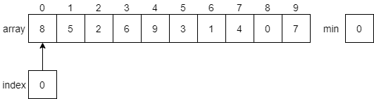
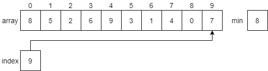
Let’s look at a few steps in this process to see how it works. First, the algorithm will search through the array to find the minimum value. It will start by looking at index 0 as shown in the figure below.
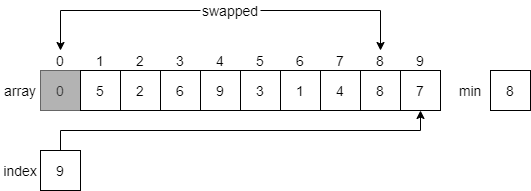
Once it reaches the end of the array, it will find that the smallest value 0 is at index 8.
Then, it will swap the minimum item with the item at index 0 of the array, placing the smallest item first. That item will now be part of the sorted array, so we’ll shade it in since we don’t want to move it again.
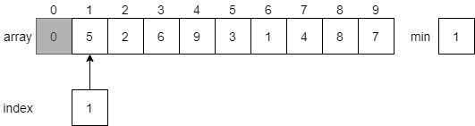
Next, it will reset index to 1, and start searching for the next smallest element in the array. Notice that this time it will not look at the element at index 0, which is part of the sorted array. Each time the algorithm resets, it will start looking at the element directly after the sorted portion of the array.
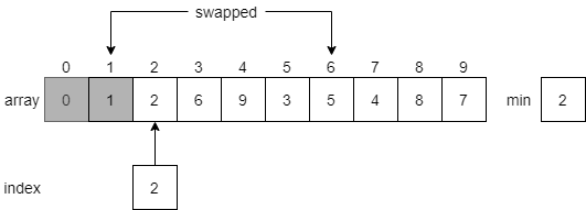
Once again, it will search through the array to find the smallest value, which will be the value 1 at index 6.
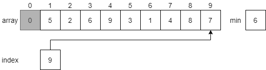
Then, it will swap the element at index 1 with the minimum element, this time at index 6. Just like before, we’ll shade in the first element since it is now part of the sorted list, and reset the index to begin at index 2
This process will repeat until the entire array is sorted in ascending order.
To describe our selection sort algorithm, we can start with these basic preconditions and postconditions.
Preconditions:
Postconditions:
We can then represent this algorithm using the following pseudocode.
function SELECTIONSORT(ARRAY)					        (1)
    loop INDEX from 0 to size of ARRAY – 2			    (2)
	  MININDEX = 0						                (3)
        # find minimum index
        loop INDEX2 from INDEX to size of ARRAY – 1		(4)
            if ARRAY[INDEX2] < ARRAY[MININDEX] then		(5)
                MININDEX = INDEX					    (6)
            end if							            (7)
        end loop							            (8)
        # swap elements
        TEMP = ARRAY[MININDEX]					        (9)
        ARRAY[MININDEX] = ARRAY[INDEX]				    (10)
        ARRAY[INDEX] = TEMP					            (11)
    end loop								            (12)
end function								            (13)
In this code, we begin by looping through every element in the array except the last one, as seen on line 2. We don’t include this one because if the rest of the array is sorted properly, then the last element must be the maximum value.
Lines 3 through 8 are basically the same as what we saw in our findMin function earlier. It will find the index of the minimum value starting at INDEX through the end of the array. Notice that we are starting at INDEX instead of the beginning. As the outer loop moves through the array, the inner loop will consider fewer and fewer elements. This is because the front of the array contains our sorted elements, and we don’t want to change them once they are in place.
Lines 9 through 11 will then swap the elements at INDEX and MININDEX, putting the smallest element left in the array at the position pointed to by index.
We can describe the invariant of our outer loop as follows:
index is sorted in ascending order.The second part of the loop invariant is very important. Without that distinction, we could simply place new values into the array before index and satisfy the first part of the invariant. It is always important to specify that the array itself still contains the same elements as before.
Let’s look at the time complexity of the selection sort algorithm, just so we can get a feel for how much time this operation takes.
First, we must determine if there is a worst-case input for selection sort. Can we think of any particular input which would require more steps to complete?
In this case, each iteration of selection sort will look at the same number of elements, no matter what they are. So there isn’t a particular input that would be considered worst-case. We can proceed with just the general case.
In each iteration of the algorithm we need to search for the minimum value of the remaining elements in the container. If the container has $N$ elements, we would follow the steps below.
This process continues until we have sorted all of the elements in the array. The number of steps will be:
$$ N + (N – 1) + (N – 2) + … + 2 + 1 $$
While it takes a bit of math to figure out exactly what that means, we can use some intuition to determine an approximate value. For example we could pair up the values like this:
$$ N + [(N – 1) + 1] + [(N – 2) + 2] + … $$
When we do that, we’ll see that we can create around $N / 2$ pairs, each one with the value of $N$. So a rough approximation of this value is $N * (N / 2)$, which is $N^2 / 2$. When analyzing time complexity, we would say that this is “on the order of $N^2$” time. Put another way, if the size of $N$ doubles, we would expect the number of steps to go up by a factor of $4$, since $(2 * N)^2 = 4N$.
Later on, we’ll come back to this and compare the time complexity of each sorting algorithm and searching algorithm to see how they stack up against each other.
Next, let’s look at another sorting algorithm, bubble sort. The basic idea behind bubble sort is to continuously iterate through the array and swap adjacent elements that are out of order. As a side effect of this process, the largest element in the array will be “bubbled” to the end of the array after the first iteration. Subsequent iterations will do the same for each of the next largest elements, until eventually the entire list is sorted.
Wikipedia includes a great animation that shows this process:
 ^[File:Bubble-sort-example-300px.gif. (2019, June 12). Wikimedia Commons, the free media repository. Retrieved 22:36, March 23, 2020 from https://commons.wikimedia.org/w/index.php?title=File:Bubble-sort-example-300px.gif&oldid=354097364.
]
In this animation, the two red boxes slowly move through the array, comparing adjacent elements. If the elements are not in the correct order (that is, the first element is larger than the second element), then it will swap them. Once it reaches the end, the largest element, 8, will be placed at the end and locked in place.
^[File:Bubble-sort-example-300px.gif. (2019, June 12). Wikimedia Commons, the free media repository. Retrieved 22:36, March 23, 2020 from https://commons.wikimedia.org/w/index.php?title=File:Bubble-sort-example-300px.gif&oldid=354097364.
]
In this animation, the two red boxes slowly move through the array, comparing adjacent elements. If the elements are not in the correct order (that is, the first element is larger than the second element), then it will swap them. Once it reaches the end, the largest element, 8, will be placed at the end and locked in place.
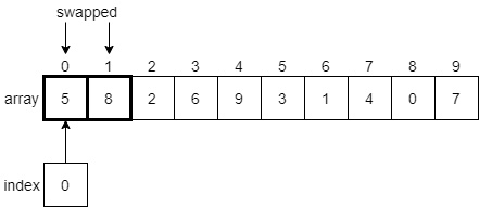
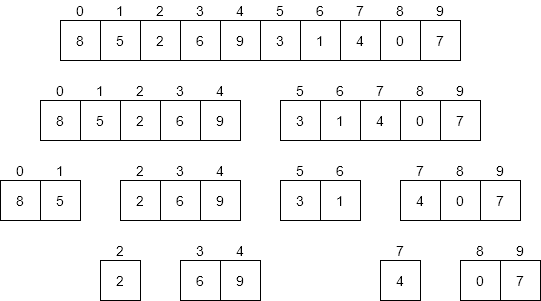
Let’s walk through a few steps of this process and see how it works. We’ll use the array we used previously for selection sort, just to keep things simple. At first, the array will look like the diagram below.
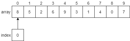
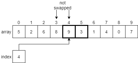
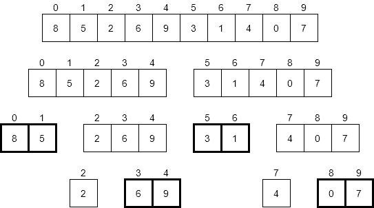
We’ll begin with the index variable pointing at index 0. Our algorithm should compare the values at index 0 and index 1 and see if they need to be swapped. We’ll put a bold border around the elements we are currently comparing in the figure below.
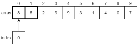
Since the element at index 0 is 8, and the element at index 1 is 5, we know that they must be swapped since 8 is greater than 5. We need to swap those two elements in the array, as shown below.
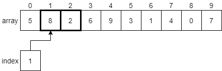
Once those two elements have been swapped, the index variable will be incremented by 1, and we’ll look at the elements at indexes 1 and 2 next.
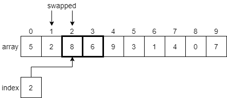
Since 8 is greater than 2, we’ll swap these two elements before incrementing index to 2 and comparing the next two elements.
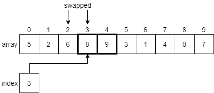
Again, we’ll find that 8 is greater than 6, so we’ll swap these two elements and move on to index 3.
Now we are looking at the element at index 3, which is 8, and the element at index 4, which is 9. In this case, 8 is less than 9, so we don’t need to swap anything. We’ll just increment index by 1 and look at the elements at indexes 4 and 5.
As we’ve done before, we’ll find that 9 is greater than 3, so we’ll need to swap those two items. In fact, as we continue to move through the array, we’ll find that 9 is the largest item in the entire array, so we’ll end up swapping it with every element down to the end of the array. At that point, it will be in its final position, so we’ll lock it and restart the process again.
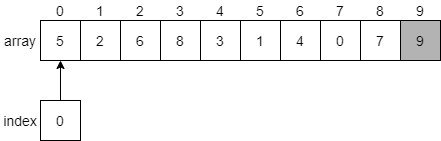
After making a second pass through the array, swapping elements that must be swapped as we find them, we’ll eventually get to the end and find that 8 should be placed at index 8 since it is the next largest value in the array.
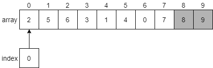
We can then continue this process until we have locked each element in place at the end of the array.
To describe our bubble algorithm, we can start with these basic preconditions and postconditions.
Preconditions:
Postconditions:
We can then represent this algorithm using the following pseudocode.
function BUBBLESORT(ARRAY)							            (1)
    # loop through the array multiple times
    loop INDEX from 0 to size of ARRAY – 1					    (2)
        # consider every pair of elements except the sorted ones
        loop INDEX2 from 0 to size of ARRAY – 2 – INDEX			(3)
            if ARRAY[INDEX2] > ARRAY[INDEX2 + 1] then			(4)
                # swap elements if they are out of order
                TEMP = ARRAY[INDEX2]						    (5)
                ARRAY[INDEX2] = ARRAY[INDEX2 + 1]				(6)
                ARRAY[INDEX2 + 1] = TEMP					    (7)
            end if
        end loop
    end loop
end function
In this code, we begin by looping through every element in the array, as seen on line 2. Each time we run this outer loop, we’ll lock one additional element in place at the end of the array. Therefore, we need to run it once for each element in the array.
On line 3, we’ll start at the beginning of the array and loop to the place where the sorted portion of the array begins. We know that after each iteration of the outer loop, the value index will represent the number of locked elements at the end of the array. We can subtract that value from the end of the array to find where we want to stop.
Line 4 is a comparison between two adjacent elements in the array starting at the index index2. If they are out of order, we use lines 5 through 7 to swap them. That’s really all it takes to do a bubble sort!
Looking at this code, we can describe the invariant of our outer loop as follows:
index elements in the array are in sorted order, andNotice how this differs from selection sort, since it places the sorted elements at the beginning of the array instead of the end. However, the result is the same, and by the end of the program we can show that each algorithm has fully sorted the array.
Once again, let’s look at the time complexity of the bubble sort algorithm and see how it compares to selection sort.
Bubble sort is a bit trickier to analyze than selection sort, because there are really two parts to the algorithm:
Let’s look at each one individually. First, is there a way to reduce the number of comparisons made by this algorithm just by changing the input? As it turns out, there isn’t anything we can do to change that based on how it is written. The number of comparisons only depends on the size of the array. In fact, the analysis is exactly the same as selection sort, since each iteration of the outer loop does one fewer comparison. Therefore, we can say that bubble sort has time complexity on the order of $N^2$ time when it comes to comparisons.
What about swaps? This is where it gets a bit tricky. What would be the worst-case input for the bubble sort algorithm, which would result in the largest number of swaps made?
Consider a case where the input is sorted in descending order. The largest element will be first, and the smallest element will be last. If we want the result to be sorted in ascending order, we would end up making $N - 1$ swaps to get the first element to the end of the array, then $N - 2$ swaps for the second element, and so on. So, once again we end up with the same series as before:
$$ (N – 1) + (N – 2) + … + 2 + 1. $$
In the worst-case, we’ll also end up doing on the order of $N^2$ swaps, so bubble sort has a time complexity on the order of $N^2$ time when it comes to swaps as well.
It seems that both bubble sort and selection sort are in the same order of time complexity, meaning that each one will take roughly the same amount of time to sort the same array. Does that tell us anything about the process of sorting an array?
Here’s one way to think about it: what if we decided to compare each element in an array to every other element? How many comparisons would that take? We can use our intuition to know that each element in an array of $N$ elements would require $N – 1$ comparisons, so the total number of comparisons would be $N * (N – 1)$, which is very close to $N^2$.
Of course, once we’ve compared each element to every other element, we’d know exactly where to place them in a sorted array. One possible conclusion we could make is that there isn’t any way to sort an array that runs much faster than an algorithm that runs in the order of $N^2$ time.
Thankfully, that conclusion is incorrect! There are several other sorting algorithms we can use that allow us to sort an array much more quickly than $N^2$ time. Let’s take a look at those algorithms and see how they work!
Another commonly used sorting algorithm is merge sort. Merge sort uses a recursive, divide and conquer approach to sorting, which makes it very powerful. It was actually developed to handle sorting data sets that were so large that they couldn’t fit on a single memory device, way back in the early days of computing.
The basic idea of the merge sort algorithm is as follows:
Once again, Wikipedia has a great animation showing this process:
 ^[File:Merge-sort-example-300px.gif. (2020, February 22). Wikimedia Commons, the free media repository. Retrieved 00:06, March 24, 2020 from https://commons.wikimedia.org/w/index.php?title=File:Merge-sort-example-300px.gif&oldid=397192885.]
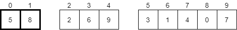
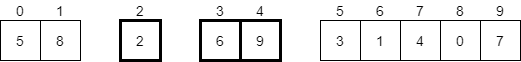
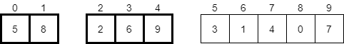
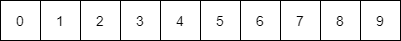
Let’s walk through a simple example and see how it works. First, we’ll start with the same initial array as before, shown in the figure below. To help us keep track, we’ll refer to this function call using the array indexes it covers. It will be mergeSort(0, 9).

Since this array contains more than 2 elements, we won’t be able to sort it quickly. Instead, we’ll divide it in half, and sort each half using merge sort again. Let’s continue the process with the first half of the array. We’ll use a thick outline to show the current portion of the array we are sorting, but we’ll retain the original array indexes to help keep track of everything.

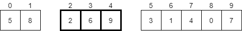
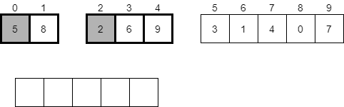
Now we are in the first recursive call, mergeSort(0, 4),which is looking at the first half of the original array. Once again, we have more than 2 elements, so we’ll split it in half and recursively call mergeSort(0, 1) first.

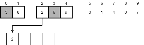
At this point, we now have an array with just 2 elements. We can use one of our base cases to sort that array by swapping the two elements, if needed. In this case, we should swap them, so we’ll get the result shown below.
Now that the first half of the smaller array has been sorted, our recursive call mergeSort(0, 1) will return and we’ll look at the second half of the smaller array in the second recursive call, mergeSort(2, 4), as highlighted below.
As we’ve seen before, this array has more than 2 elements, so we’ll need to divide it in half and recursively call the function again. First, we’ll call mergeSort(2, 2).
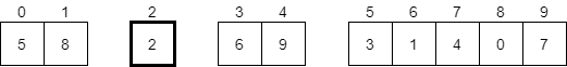
In this case, the current array we are considering contains a single element, so it is already sorted. Therefore, the recursive call to mergeSort(2, 2) will return quickly, and we’ll consider the second part of the smaller array in mergeSort(3, 4), highlighted below.
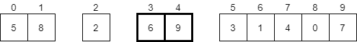
Here, we have 2 elements, and this time they are already sorted. So, we don’t need to do anything, and our recursive call to mergeSort(3, 4) will return. At this point, we will be back in our call to mergeSort(2, 4), and both halves of that array have been sorted. We’re back to looking at the highlighted elements below.
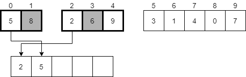
Now we have to merge these two arrays together. Thankfully, since they are sorted, we can follow this simple process:
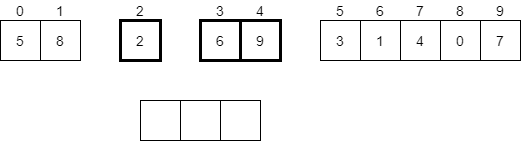
Let’s take a look at what that process would look like. First, we’ll create a new temporary array to store the result.
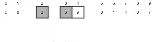
Next, we will look at the first element in each of the two sorted halves of the original array. In this case, we’ll compare 2 and 6, which are highlighted below.
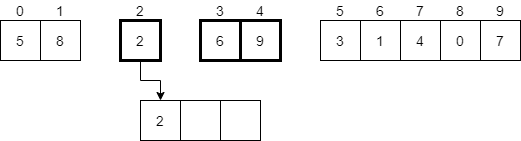
Now we should pick the smaller of those two values, which will be 2. That value will be placed in the new temporary array at the very beginning.
Next, we should look at the remaining halves of the array. Since the first half is empty, we can just place the remaining elements from the second half into the temporary array.
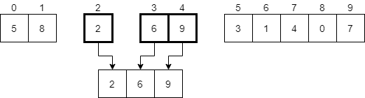
Finally, we should replace the portion of the original array that we are looking at in this recursive call with the temporary array. In most cases, we’ll just copy these elements into the correct places in the original array. In the diagram, we’ll just replace them.

There we go! We’ve now completed the recursive call mergeSort(2, 4). We can return from that recursive call and go back to mergeSort(0, 4).
Since both halves of the array in mergeSort(0, 4) are sorted, we must do the merge process again. We’ll start with a new temporary array and compare the first element in each half.
At this point, we’ll see that 2 is the smaller of those elements, so we’ll place it in the first slot in the temporary array and consider the next element in the second half.
Next, we’ll compare the values 5 and 6, and see that 5 is smaller. It should be placed in the next available element in our temporary array and we should continue onward.
We’ll repeat this process again, placing the 6 in the temporary array, then the 8, then finally the 9. After completing the merge process, we’ll have the following temporary array.
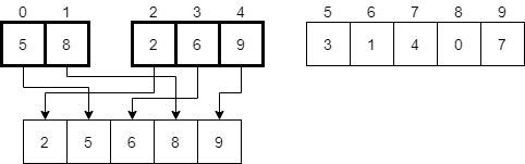
Finally, we’ll replace the original elements with the now merged elements in the temporary array.
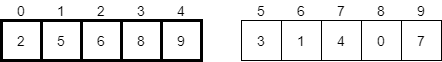
There we go! We’ve now completed the process in the mergeSort(0, 4) recursive call. Once that returns, we’ll be back in our original call to mergeSort(0, 9). In that function, we’ll recursively call the process again on the second half of the array using mergeSort(5, 9).
Hopefully by now we understand that it will work just like we intended, so by the time that recursive call returns, we’ll now have the second half of the array sorted as well.
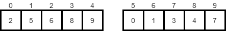
The last step in the original mergeSort(0, 9) function call is to merge these two halves together. So, once again, we’ll follow that same process as before, creating a new temporary array and moving through the elements in each half, placing the smaller of the two in the new array. Once we are done, we’ll end up with a temporary array that has been populated as shown below.
Finally, we’ll replace the elements in the original array with the ones in the temporary array, resulting in a completely sorted result.
Now that we’ve seen how merge sort works by going through an example, let’s look at the pseudocode of a merge sort function.
function MERGESORT(ARRAY, START, END)			(1)
    # base case size == 1
    if END - START + 1 == 1 then				(2)
        return						            (3)
    end if							            (4)
    # base case size == 2
    if END - START + 1 == 2 then				(5)
        # check if elements are out of order
        if ARRAY[START] > ARRAY[END] then		(6)
            # swap if so
            TEMP = ARRAY[START]				    (7)
            ARRAY[START] = ARRAY[END]			(8)
            ARRAY[END] = TEMP				    (9)
        end if						            (10)
        return						            (11)
    end if							            (12)
    # find midpoint
    HALF = int((START + END) / 2)			    (13)
    # sort first half
    MERGESORT(ARRAY, START, HALF)			    (14)
    # sort second half
    MERGESORT(ARRAY, HALF + 1, END)			    (15)
    # merge halves
    MERGE(ARRAY, START, HALF, END)			    (16)
end function							        (17)
This function is a recursive function which has two base cases. The first base case is shown in lines 2 through 4, where the size of the array is exactly 1. In that case, the array is already sorted, so we just return on line 3 without doing anything.
The other base case is shown in lines 5 through 11. In this case, the element contains just two elements. We can use the if statement on line 6 to check if those two elements are in the correct order. If not, we can use lines 7 through 9 to swap them, before returning on line 11.
If neither of the base cases occurs, then we reach the recursive case starting on line 13. First, we’ll need to determine the midpoint of the array , which is just the average of the start and end variables. We’ll need to remember to make sure that value is an integer by truncating it if needed.
Then, on lines 14 and 15 we make two recursive calls, each one focusing on a different half of the array. Once each of those calls returns, we can assume that each half of the array is now sorted.
Finally, in line 16 we call a helper function known as merge to merge the two halves together. The pseudocode for that process is below.
function MERGE(ARRAY, START, HALF, END)			    (1)
    TEMPARRAY = new array[END – START + 1]			(2)
    INDEX1 = START							        (3)
    INDEX2 = HALF + 1						        (4)
    NEWINDEX = 0							        (5)
    loop while INDEX1 <= HALF and INDEX2 <= END		(6)
        if ARRAY[INDEX1] < ARRAY[INDEX2] then		(7)
            TEMPARRAY[NEWINDEX] = ARRAY[INDEX1]		(8)
            INDEX1 = INDEX1 + 1					    (9)
        else								        (10)
            TEMPARRAY[NEWINDEX] = ARRAY[INDEX2]		(11)
            INDEX2 = INDEX2 + 1					    (12)
        end if							            (13)
        NEWINDEX = NEWINDEX + 1					    (14)
    end loop								        (15)
    loop while INDEX1 <= HALF					    (16)
        TEMPARRAY[NEWINDEX] = ARRAY[INDEX1]			(17)
        INDEX1 = INDEX1 + 1					        (18)
        NEWINDEX = NEWINDEX + 1					    (19)
    end loop								        (20)
    loop while INDEX2 <= END					    (21)
        TEMPARRAY[NEWINDEX] = ARRAY[INDEX2]			(22)
        INDEX2 = INDEX2 + 1					        (23)
        NEWINDEX = NEWINDEX + 1					    (24)
    end loop								        (25)
    loop INDEX from 0 to size of TEMPARRAY – 1		(26)
        ARRAY[START + INDEX] = TEMPARRAY[INDEX]		(27)
    end loop								        (28)
end function								        (29)
The merge function begins by creating some variables. The tempArray will hold the newly merged array. Index1 refers to the element in the first half that is being considered, while index2 refers to the element in the second half. Finally, newIndex keeps track of our position in the new array.
The first loop starting on line 6 will continue operating until one half or the other has been completely added to the temporary array. It starts by comparing the first element in each half of the array. Then, depending on which one is smaller, it will place the smaller of the two in the new array and increment the indexes.
Once the first loop has completed, there are two more loops starting on lines 16 and 21. However, only one of those loops will actually execute, since only one half of the array will have any elements left in it to be considered. These loops will simply copy the remaining elements to the end of the temporary array.
Finally, the last loop starting on line 26 will copy the elements from the temporary array back into the source array. At this point, they will be properly merged in sorted order.
Now that we’ve reviewed the pseudocode for the merge sort algorithm, let’s see if we can analyze the time it takes to complete. Analyzing a recursive algorithm requires quite a bit of math and understanding to do it properly, but we can get a pretty close answer using a bit of intuition about what it does.
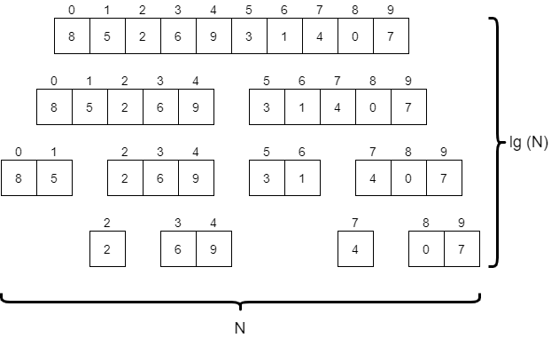
For starters, let’s consider a diagram that shows all of the different recursive calls made by merge sort, as shown below.
The first thing we should do is consider the worst-case input for merge sort. What would that look like? Put another way, would the values or the ordering of those values change anything about how merge sort operates?
The only real impact that the input would have is on the number of swaps made by merge sort. If we had an input that caused each of the base cases with exactly two elements to swap them, that would be a few more steps than any other input. Consider the highlighted entries below.
If each of those pairs were reversed, we’d end up doing that many swaps. So, how many swaps would that be? As it turns out, a good estimate would be $N / 2$ times. If we have an array with exactly 16 elements, there are at most 8 swaps we could make. With 10 elements, we can make at most 4. So, the number of swaps is on the order of N time complexity.
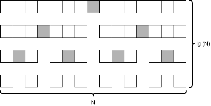
What about the merge operation? How many steps does that take? This is a bit trickier to answer, but let’s look at each row of the diagram above. Across all of the calls to merge sort on each row, we’ll end up merging all $N$ elements in the original array at least once. Therefore, we know that it would take around $N$ steps for each row in the diagram. We’ll just need to figure out how many rows there are.
A better way to phrase that question might be “how many times can we recursively divide an array of $N$ elements in half?” As it turns out, the answer to that question lies in the use of the logarithm.
The logarithm is the inverse of exponentiation. For example, we could have the exponentiation formula:
$$ \text{base}^{\text{exponent}} = \text{power} $$
The inverse of that would be the logarithm $$ \text{log}_{\text{base}}(\text{power}) = \text{exponent} $$
So, if we know a value and base, we can determine the exponent required to raise that base to the given value.
In this case, we would need to use the logarithm with base $2$, since we are dividing the array in half each time. So, we would say that the number of rows in that diagram, or the number of levels in our tree would be on the order of $\text{log}_2(N)$. In computer science, we typically write $\text{log}_2$ as $\text{lg}$, so we’ll say it is on the order of $\text{lg}(N)$.
To get an idea of how that works, consider the case where the array contains exactly $16$ elements. In that case, the value $\text{lg}(16)$ is $4$, since $2^4 = 16$. If we use the diagram above as a model, we can draw a similar diagram for an array containing $16$ elements and find that it indeed has $4$ levels.
If we double the size of the array, we’ll now have $32$ elements. However, even by doubling the size of the array, the value of $\text{lg}(32)$ is just $5$, so it has only increased by $1$. In fact, each time we double the size of the array, the value of $\text{lg}(N)$ will only go up by $1$.
With that in mind, we can say that the merge operation runs on the order of $N * \text{lg}(N)$ time. That is because there are ${\text{lg}(N)}$ levels in the tree, and each level of the tree performs $N$ operations to merge various parts of the array together. The diagram below gives a good graphical representation of how we can come to that conclusion.
Putting it all together, we have $N/2$ swaps, and $N * \text{lg}(N)$ steps for the merge. Since the value $N * \text{lg}(N)$ is larger than $N$, we would say that total running time of merge sort is on the order of $N * \text{lg}(N)$.
Later on in this chapter we’ll discuss how that compares to the running time of selection sort and bubble sort and how that impacts our programs.
The last sorting algorithm we will review in this module is quicksort. Quicksort is another example of a recursive, divide and conquer sorting algorithm, and at first glance it may look very similar to merge sort. However, quicksort uses a different process for dividing the array, and that can produce some very interesting results.
The basic idea of quicksort is as follows:
pivotValue. This value could be any random value in the array. In our implementation, we’ll simply use the last value.pivotValuepivotValuepivotValue in between those two parts. We’ll call the index of pivotValue the pivotIndex.pivotIndex – 1pivotIndex + 1 to the endAs with all of the other examples we’ve looked at in this module, Wikipedia provides yet another excellent animation showing this process.
 ^[File:Sorting quicksort anim.gif. (2019, July 30). Wikimedia Commons, the free media repository. Retrieved 01:14, March 24, 2020 from https://commons.wikimedia.org/w/index.php?title=File:Sorting_quicksort_anim.gif&oldid=359998181.]
Let’s look at an example of the quicksort algorithm in action to see how it works. Unlike the other sorting algorithms we’ve seen, this one may appear to be just randomly swapping elements around at first glance. However, as we move through the example, we should start to see how it achieves a sorted result, usually very quickly!
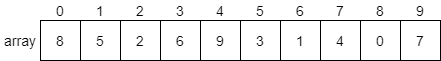
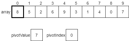
We can start with our same initial array, shown below.
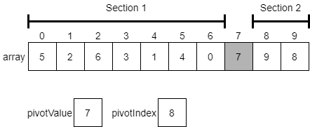
The first step is to choose a pivot value. As we discussed above, we can choose any random value in the array. However, to make it simple, we’ll just use the last value. We will create two variables, pivotValue and pivotIndex, to help us keep track of things. We’ll set pivotValue to the last value in the array, and pivotIndex will initially be set to 0. We’ll see why in a few steps.
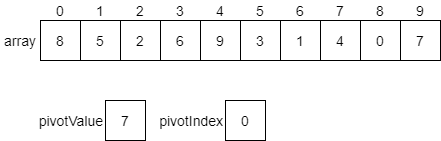
Now, the algorithm will iterate across each element in the array, comparing it with the value in pivotValue. If that value is less than or equal to the pivotValue, we should swap the element at pivotIndex with the value we are looking at in the array. Let’s see how this would work.
We’d start by looking at the value at index 0 of the array, which is 8. Since that value is greater than the pivotValue, we do nothing and just look at the next item.
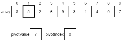
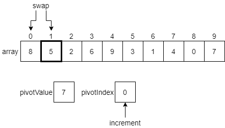
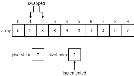
Here, we are considering the value 5, which is at index 1 in the array. In this case, that value is less than or equal to the pivotValue. So, we want to swap the current element with the element at our pivotIndex, which is currently 0. Once we do that, we’ll also increment our pivotIndex by 1. The diagram below shows these changes before they happen.
Once we make those changes, our array should look like the following diagram, and we’ll be ready to examine the value at index 2.
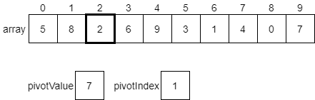
Once again, the value 2 at index 2 of the array is less than or equal to the pivot value. So, we’ll swap them, increment pivotValue, and move to the next element.
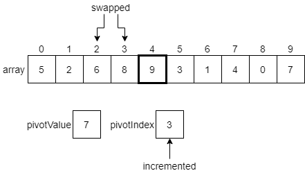
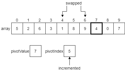
We’ll continue this process, comparing the next element in the array with the pivotValue, and then swapping that element and the element at the pivotIndex if needed, incrementing the pivotIndex after each swap. The diagrams below show the next few steps. First, since 6 is less than or equal to our pivotValue, we’ll swap it with the pivot index and increment.
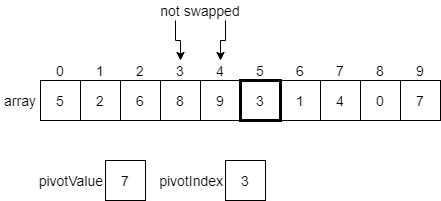
However, since 9 is greater than the pivot index, we’ll just leave it as is for now and move to the next element.
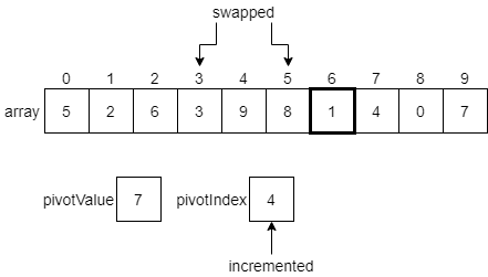
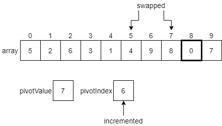
3 is less than or equal to the pivot value, so we’ll swap the element at index 3 with the 3 at index 5.
We’ll see that the elements at indexes 6, 7 and 8 are all less than or equal to the pivot value. So, we’ll end up making some swaps until we reach the end of the list.
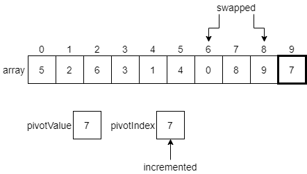
Finally, we have reached the end of the array, which contains our pivotValue in the last element. Thankfully, we can just continue our process one more step. Since the pivotValue is less than or equal to itself, we swap it with the element at the pivotIndex, and increment that index one last time.
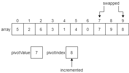
At this point, we have partitioned the initial array into two sections. The first section contains all of the values which are less than or equal to the pivot value, and the second section contains all values greater than the pivot value.
This demonstrates the powerful way that quicksort can quickly partition an array based on a pivot value! With just a single pass through the array, we have created our two halves and done at least some preliminary sorting. The last step is to make two recursive calls to quicksort, one that sorts the items from the beginning of the array through the element right before the pivotValue. The other will sort the elements starting after the pivotValue through the end of the array.
Once each of those recursive calls is complete, the entire array will be sorted!
Now that we’ve seen an example of how quicksort works, let’s walk through the pseudocode of a quicksort function. The function itself is very simple, as shown below.
function QUICKSORT(ARRAY, START, END)			(1)
    # base case size <= 1
    if START >= END then					    (2)
        return						            (3)
    end if							            (4)
    PIVOTINDEX = PARTITION(ARRAY, START, END)	(5)
    QUICKSORT(ARRAY, START, PIVOTINDEX – 1)		(6)
    QUICKSORT(ARRAY, PIVOTINDEX + 1, END)		(7)
end function							        (8)
This implementation of quicksort uses a simple base case on lines 2 through 4 to check if the array is either empty, or contains one element. It does so by checking if the START index is greater than or equal to the END index. If so, it can assume the array is sorted and just return it without any additional changes.
The recursive case is shown on lines 5 – 7. It simply uses a helper function called partition on line 5 to partition the array based on a pivot value. That function returns the location of the pivot value, which is stored in pivotIndex. Then, on lines 6 and 7, the quicksort function is called recursively on the two partitions of the array, before and after the pivotIndex. That’s really all there is to it!
Let’s look at one way we could implement the partition function, shown below in pseudocode.
function PARTITION(ARRAY, START, END)			(1)
    PIVOTVALUE = ARRAY[END]				        (2)
    PIVOTINDEX = START					        (3)
    loop INDEX from START to END				(4)
        if ARRAY[INDEX] <= PIVOTVALUE			(5)
            TEMP = ARRAY[INDEX]        		    (6)
            ARRAY[INDEX] = ARRAY[PIVOTINDEX]	(7)
            ARRAY[PIVOTINDEX] = TEMP			(8)
            PIVOTINDEX = PIVOTINDEX + 1		    (9)
        end if						            (10)
    end loop							        (11)
    return PIVOTINDEX – 1					    (12)
This function begins on lines 2 and 3 by setting initial values for the pivotValue by choosing the last element in the array, and then setting the pivotIndex to 0. Then, the loop on lines 4 through 11 will look at each element in the array, determine if it is less than or equal to pivotValue, and swap that element with the element at pivotIndex if so, incrementing pivotIndex after each swap.
At the end, the value that was originally at the end of the array will be at location pivotIndex – 1, so we will return that value back to the quicksort function so it can split the array into two parts based on that value.
To wrap up our analysis of the quicksort algorithm, let’s take a look at the time complexity of the algorithm. Quicksort is a very difficult algorithm to analyze, especially since the selection of the pivot value is random and can greatly affect the performance of the algorithm. So, we’ll talk about quicksort’s time complexity in terms of two cases, the worst case and the average case. Let’s look at the average case first
What would the average case of quicksort look like? This is a difficult question to answer and requires a bit of intuition and making a few assumptions. The key really lies in how we choose our pivot value.
First, let’s assume that the data in our array is equally distributed. This means that the values are evenly spread between the lowest value and the highest value, with no large clusters of similar values anywhere. While this may not always be the case in the real world, often we can assume that our data is somewhat equally distributed.
Second, we can also assume that our chosen pivot value is close to the average value in the array. If the array is equally distributed and we choose a value at random, we have a $50%$ chance of that value being closer to the average than either the minimum or the maximum value, so this is a pretty safe assumption.
With those two assumptions in hand, we see that something interesting happens. If we choose the average value as our pivot value, quicksort will perfectly partition the array into two equal sized halves! This is a great result, because it means that each recursive call to the function will be working with data that is half the initial array.
If we consider an array that initially contains $15$ elements, and make sure that we always choose the average element as our pivot point, we’d end up with a tree of recursive calls that resembles the diagram below.
In this diagram, we see that each level of the tree looks at around $N$ elements. (It is actually fewer, but not by a significant amount so we can just round up to $N$ each time). We also notice that there are 4 levels to the tree, which is closely approximated by $\text{lg}(N)$. This is the same result we observed when analyzing the merge sort algorithm earlier in this module.
So, in the average case, we’d say that quicksort runs in the order of $N * \text{lg}(N)$ time.
To consider the worst-case situation for quicksort, we must come up with a way to define what the worst-case input would be. It turns out that the selection of our pivot value is the key here.
Consider the situation where the pivot value is chosen to be the maximum value in the array. What would happen in that case?
Looking at the code, we would see that each recursive call would contain one empty partition, and the other partition would be just one less than the size of the original array. So, if our original array only contained 8 elements, our tree recursion diagram would look similar to the following.
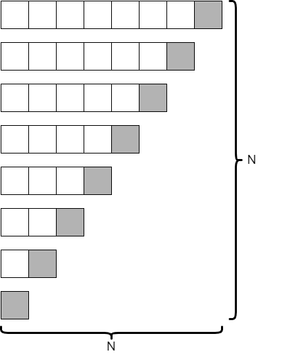
This is an entirely different result! In this case, since we are only reducing the size of our array by 1 at each level, it would take $N$ recursive calls to complete. However, at each level, we are looking at one fewer element. Is this better or worse than the average case?
It turns out that it is much worse. As we learned in our analysis of selection sort and bubble sort, the series
$$ N + (N – 1) + (N – 2) + … + 2 + 1 $$
is best approximated by $N^2$. So, we would say that quicksort runs in the order of $N^2$ time in the worst case. This is just as slow as selection sort and bubble sort! Why would we ever call it “quicksort” if it isn’t any faster?
Thankfully, in practice, it is very rare to run into this worst-case performance with quicksort, and in fact most research shows that quicksort is often the fastest of the four sorting algorithms we’ve discussed so far. In the next section, we’ll discuss these performance characteristics a bit more.
This result highlights why it is important to consider both the worst case and average case performance of our algorithms. Many times we’ll write an algorithm that runs well most of the time, but is susceptible to poor performance when given a particular worst-case input.
We introduced four sorting algorithms in this chapter: selection sort, bubble sort, merge sort, and quicksort. In addition, we performed a basic analysis of the time complexity of each algorithm. In this section, we’ll revisit that topic and compare sorting algorithms based on their performance, helping us understand what algorithm to choose based on the situation.
The list below shows the overall result of our time complexity analysis for each algorithm.
We have expressed the amount of time each algorithm takes to complete in terms of the size of the original input $N$. But how does $N^2$ compare to $N * \text{lg}(N)$?
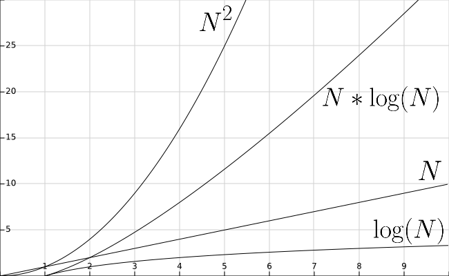
One of the easiest ways to compare two functions is to graph them, just like we’ve learned to do in our math classes. The diagram below shows a graph containing the functions $N$, $N^2$, and $N * \text{lg}(N)$.
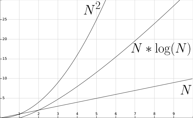
First, notice that the scale along the X axis (representing values of $N$) goes from 0 to 10, while the Y axis (representing the function outputs) goes from 0 to 30. This graph has been adjusted a bit to better show the relationship between these functions, but in actuality they have a much steeper slope than is shown here.
As we can see, the value of $N^2$ at any particular place on the X axis is almost always larger than $N * \text{lg}(N)$, while that function’s output is almost always larger than $N$ itself. We can infer from this that functions which run in the order of $N^2$ time will take much longer to complete than functions which run in the order of $N * \text{lg}(N)$ time. Likewise, the functions which run in the order of $N * \text{lg}(N)$ time themselves are much slower than functions which run in linear time, or in the order of $N$ time.
Based on that assessment alone, we might conclude that we should always use merge sort! It is guaranteed to run in $N * \text{lg}(N)$ time, with no troublesome worst-case scenarios to consider, right? Unfortunately, as with many things in the real world, it isn’t that simple.
The choice of which sorting algorithm to use in our programs largely comes down to what we know about the data we have, and how that information can impact the performance of the algorithm. This is true for many other algorithms we will write in this class. Many times there are multiple methods to perform a task, such as sorting, and the choice of which method we use largely depends on what we expect our input data to be.
For example, consider the case where our input data is nearly sorted. In that instance, most of the items are in the correct order, but a few of them, maybe less than $10%$, are slightly out of order. In that case, what if we used a version of bubble sort that was optimized to stop sorting as soon as it makes a pass through the array without swapping any elements? Since only a few elements are out of order, it may only take a few passes with bubble sort to get them back in the correct places. So even though bubble sort runs in $N^2$ time, the actual time may be much quicker.
Likewise, if we know that our data is random and uniformly distributed, we might want to choose quicksort. Even though quicksort has very slow performance in the worst case, if our data is properly random and distributed, research shows that it will have better real-world performance than most other sorting algorithms in that instance.
Finally, what if we know nothing about our input data? In that case, we might want to choose merge sort as the safe bet. It is guaranteed to be no worse than $N * \text{lg}(N)$ time, even if the input is truly bad. While it might not be as fast as quicksort if the input is random, it won’t run the risk of being slow, either.
Now that we’ve learned how to sort the data in our container, let’s go back and revisit the concept of searching once again. Does our approach change when we know the data has been sorted?
Our intuition tells us that it should. Recall that we discussed how much easier it would be to find a particular paper in a sorted filing cabinet rather than just searching through a random pile of papers on the floor. The same concept applies to data in our programs.
The most commonly used searching algorithm when dealing with sorted data is binary search. The idea of the algorithm is to compare the value in the middle of the container with the value we are looking for. In this case, let’s assume the container is sorted in ascending order, so the smaller elements are before the larger ones. If we compare our desired value with the middle value, there are three possible outcomes:
Once an occurrence of the desired value is found, we can also look at the values before it to see if there any more of the desired values in the container. Since it is sorted, they should all be grouped together. If we want our algorithm to return the index of the first occurrence of the desired value, we can simply move toward the front of the array until we find that first occurrence.
Let’s work through a quick example of the binary search algorithm to see how it works in practice. Let’s assume we have the array shown in the diagram below, which is already sorted in ascending order. We wish to find out if the array contains the value 5. So, we’ll store that in our value variable. We also have variables start and end representing the first and last index in the array that we are considering.
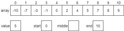
First, we must calculate the middle index of the array. To do that, we can use the following formula.
$$ \text{int}((\text{start} + \text{end}) / 2) $$
In this case, we’ll find that the middle index is 5.

Next, we’ll compare our desired value with the element at the middle index, which is 2. Since our desired value 5 is greater than 2, we know that 5 must be present in the second half of the array. We will then update our starting value to be one greater than the middle element and start over. In practice, this could be done either iteratively or recursively. We’ll see both implementations later in this section. The portion of the array we are ignoring has been given a grey background in the diagram below.
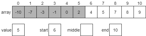
Once again, we’ll start by calculating a new middle index. In this case, it will be 8.

The value at index 8 is 7, which is greater than our desired value 5. So we know that 5 should be in the first half of the array from index 6 through 10. We need to update the end variable to be one less than middle and try once again.
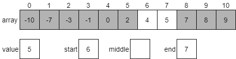
We’ll first calculate the middle index, which will be 6. This is because (6 + 7) / 2 is 6.5, but when we convert it to an integer it will be truncated, resulting in just 6.

Since the value at index 6 is 4, which is less than our desired value 5, we know that we should be looking at the portion of the array which comes after our middle element. Once again, we’ll update our start index to be one greater than the middle and start over.
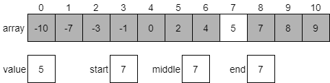
In this case, since both start and end are the same, we know that the middle index will also be 7. We can compare the value at index 7 to our desired value. As it turns out, they are a match, so we’ve found our value! We can just return middle as the index for this value. Of course, if we want to make sure it is the first instance of our desired value, we can quickly check the elements before it until we find one that isn’t our desired value. We won’t worry about that for now, but it is something that can easily be added to our code later.
The binary search algorithm is easily implemented in both an iterative and recursive function. We’ll look at both versions and see how they compare.
The pseudocode for an iterative version of binary search is shown below.
function BINARYSEARCH(ARRAY, VALUE)			    (1)
    START = 0						            (2)
    END = size of ARRAY - 1				        (3)
    loop while START <= END				        (4)
        MIDDLE = INT((START + END) / 2)		    (5)
        if ARRAY[MIDDLE] == VALUE then			(6)
            return MIDDLE					    (7)
        else if ARRAY[MIDDLE] > VALUE then		(8)
            END = MIDDLE – 1				    (9)
        else if ARRAY[MIDDLE] < VALUE then		(10)
            START = MIDDLE + 1				    (11)
        end if						            (12)
    end loop							        (13)
    return -1						            (14)
end function							        (15)
This function starts by setting the initial values of start and end on lines 2 and 3 to the first and last indexes in the array, respectively. Then, the loop starting on line 4 will repeat while the start index is less than or equal to the end index. If we reach an instance where start is greater than end, then we have searched the entire array and haven’t found our desired value. At that point the loop will end and we will return -1 on line 14.
Inside of the loop, we first calculate the middle index on line 5. Then on line 6 we check to see if the middle element is our desired value. If so, we should just return the middle index and stop. It is important to note that this function will return the index to an instance of value in the array, but it may not be the first instance. If we wanted to find the first instance, we’d add a loop at line 7 to move forward in the array until we were sure we were at the first instance of value before returning.
If we didn’t find our element, then the if statements on lines 8 and 10 determine which half of the array we should look at. Those statements update either end or start as needed, and then the loop repeats.
The recursive implementation of binary search is very similar to the iterative approach. However, this time we also include both start and end as parameters, which we update at each recursive call. The pseudocode for a recursive binary search is shown below.
function BINARYSEARCHRECURSE(ARRAY, VALUE, START, END)			       (1)
    # base case
    if START > END then								                   (2)
        return -1									                   (3)
    end if										                       (4)
    MIDDLE = INT((START + END) / 2)						               (5)
    if ARRAY[MIDDLE] == VALUE then						               (6)
        return MIDDLE								                   (7)
    else if ARRAY[MIDDLE] > VALUE then						           (8)
        return BINARYSEARCHRECURSE(ARRAY, VALUE, START, MIDDLE – 1)	   (9)
    else if ARRAY[MIDDLE] < VALUE then						           (10)
        return BINARYSEARCHRECURSE(ARRAY, VALUE, MIDDLE + 1, END)	   (11)
    end if										                       (12)
end function										                   (13)
The recursive version moves the loop’s termination condition to the base case, ensuring that it returns -1 if the start index is greater than the end index. Otherwise, it performs the same process of calculating the middle index and checking to see if it contains the desired value. If not, it uses the recursive calls on lines 9 and 11 to search the first half or second half of the array, whichever is appropriate.
Analyzing the time complexity of binary search is similar to the analysis done with merge sort. In essence, we must determine how many times it must check the middle element of the array.
In the worst case, it will continue to do this until it has determined that the value is not present in the array at all. Any time that our array doesn’t contain our desired value would be our worst-case input.
In that instance, how many times do we look at the middle element in the array? That is hard to measure. However, it might be easier to measure how many elements are in the array each time and go from there.
Consider the situation where we start with 15 elements in the array. How many times can we divide the array in half before we are down to just a single element? The diagram below shows what this might look like.
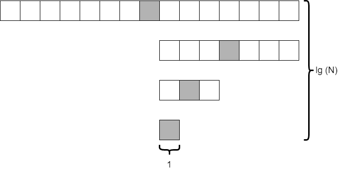
As it turns out, this is similar to the analysis we did on merge sort and quick sort. If we divide the array in half each time, we will do this $\text{lg}(N)$ times. The only difference is that we are only looking at a single element, the shaded element, at each level. So the overall time complexity of binary search is on the order of $\text{lg}(N)$. That’s pretty fast!
Let’s go back and look at the performance of our sorting algorithms, now that we know how quickly binary search can find a particular value in an array. Let’s add the function $\text{lg}(N)$ to our graph from earlier, shown below.
As we can see, the function $\text{lg}(N)$ is even smaller than $N$. So performing a binary search is much faster than a linear search, which we already know runs in the order of $N$ time.
However, performing a single linear search is still faster than any of the sorting algorithms we’ve reviewed. So when does it become advantageous to sort our data?
This is a difficult question to answer since it depends on many factors. However, a good rule of thumb is to remember that the larger the data set, or the more times we need to search for a value, the better off we are to sort the data before we search.
In the graph below, the topmost line colored in red shows the approximate running time of $10$ linear search operations, while the bottom line in black shows the running time of performing a merge sort before $10$ binary search operations.
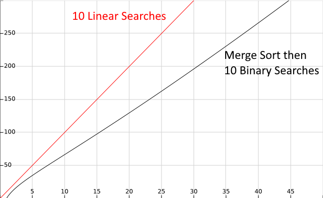
As we can see, it is more efficient to perform a merge sort, which runs in $N * \text{lg}(N)$ time, then perform $10$ binary searches running in $\text{lg}(N)$ time, than it is to perform $10$ linear searches running in $N$ time. The savings become more pronounced as the size of the input gets larger, as indicated by the X axis on the graph.
In fact, this analysis suggests that it may only take as few as 7 searches to see this benefit, even on smaller data sets. So, if we are writing a program that needs to search for a specific value in an array more than about 7 times, it is probably a good idea to sort the array before doing our searches, at least from a performance standpoint.
So far we’ve looked at sorting algorithms that run in $N * \text{lg}(N)$ time. However, what if we try to sort the data as we add it to the array? In a later course, we’ll learn how we can use an advanced data structure known as a heap to create a sorted array in nearly linear time (with some important caveats, of course)!
In this chapter, we learned how to search for values in an array using a linear search method. Then, we explored four different sorting algorithms, and compared them based on their time complexity. Finally, we learned how we can use a sorted array to perform a faster binary search and saw how we can increase our performance by sorting our array before searching in certain situations.
Searching and sorting are two of the most common operations performed in computer programs, and it is very important to have a deep understanding of how they work. Many times the performance of a program can be improved simply by using the correct searching and sorting algorithms to fit the program’s needs, and understanding when you might run into a particularly bad worst-case input.
The project in this module will involve implementing several of these algorithms in the language of your choice. As we learn about more data structures, we’ll revisit these algorithms again to discuss how they can be improved or adapted to take advantage of different structures.
Mergesort iterative without a stack
Quicksort iterative with a stack
Bubble sort recursive