What is a List?

YouTube Video

A list is a data structure that holds a sequence of data, such as the shopping list shown below. Each list has a head item and a tail item, with all other items placed linearly between the head and the tail. As we pick up items in the store, we will remove them, or cross them off the list. Likewise, if we get a text from our housemate to get some cookies, we can add them to the list as well.

^[Source: https://www.agclassroom.org/teacher/matrix/lessonplan.cfm?lpid=367]

Lists are actually very general structures that we can use for a variety of purposes. One common example is the history section of a web browser. The web browser actually creates a list of past web pages we have visited, and each time we visit a new web page it is added to the list. That way, when we check our history, we can see all the web pages we have visited recently in the order we visited them. The list also allows us to scroll through the list and select one to revisit or select another one to remove from the history altogether.

Of course, we have already seen several instances of lists so far in programming, including arrays, stacks, and queues. However, lists are much more flexible than the arrays, stacks, and queues we have studied so far. Lists allow us to add or remove items from the head, tail, or anywhere in between. We will see how we can actually implement stacks and queues using lists later in this module.

Lists in the Real World

Most of us see and use lists every day. We have a list for shopping as we saw above, but we may also have a “to do” list, a list of homework assignments, or a list of movies we want to watch. Some of us are list-makers and some are not, but we all know a list when we see it.

^[Source: https://wiki.videolan.org/index.php?title=File:Basic_playlist_default.png&oldid=59730]

However, there are other lists in the real world that we might not even think of as a list. For instance, a playlist on our favorite music app is an example of a list. A music app lets us move forward or backward in a list or choose a song randomly from a list. We can even reorder our list whenever we want.

All the examples we’ve seen for stacks and queues can be thought of as lists as well. Stacks of chairs or moving boxes, railroad trains, and cars going through a tollbooth are all examples of special types of lists.

Lists in Code

The Problem With Arrays

To this point, we have been using arrays as our underlying data structures for implementing linear data structures such as stacks and queues. Given that with stacks and queues we only put items into the array and remove from either the start or end of the data structure, we have been able to make arrays work. However, there are some drawbacks to using arrays for stacks and queues as well as for more general data structures.

1. We can run out of room in our array for our stacks or queues.
2. There is no good way to use memory efficiently. We have to use expensive “double” and “halve” capacity operations for stacks and queues when we need to use more or less memory.
3. Inserting an item into the middle of a sorted list will be very costly in memory. In an array, we will have to move several items to keep the list in order.

While drawbacks 1 and 2 above can be overcome (albeit rather awkwardly) when using arrays for stacks and queues, drawback 3 becomes a real problem when trying to use more general list structures. If we insert an item into the middle of an array, we must move several other items “down” the array to make room.

If for example, if we want to insert the number 5 into the sorted array shown below, we have to carry out several steps:

1. Find the index of the first item whose value is greater than the number we want to insert into the array. We will call this index i,
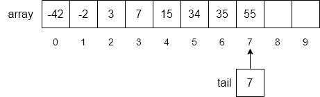
2. Shift each item from index i to the end of the list down one place location in the array,
3. Insert the new item into the array at index i, and
4. Update the index to the tail of the list.

In our example, step 1 will loop through each item of the array until we find the first number in the array greater than 5. As shown below, the number 7 is found in index 3.

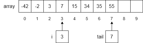
Next, we will use another loop to move each item from index i to the end of the array down by one index number as shown below.

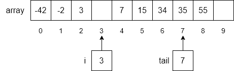
Finally, we will insert our new number, 5, into the array at index 3 and increment tail to 8.

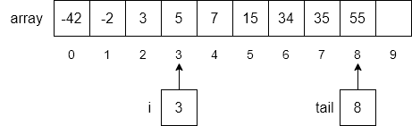
In this operation, if we have $N$ items, we either compare or move all of them, which would require $N$ operations. Of course, this operation runs in order $N$ time.

The same problem occurs when we remove an item from the array. In this case we must perform the following steps:

1. Search the array to find the first occurrence of the desired number to remove,
2. Continue searching until we find the last occurrence of the desired number to remove,
3. Shift each item after the last occurrence of our desired number “up” the array, once for each desired number being removed from the array, and
4. Update the index to the tail of the list.

A More Flexible Approach

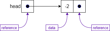
Instead of using arrays to try to hold our lists, a more flexible approach is to build our own list data structure that relies on a set of objects that are all linked together through references to each other. In the figure below we have created a list of numbers that are linked to each other. Each object contains both the number as well as a reference to the next number in the list. Using this structure, we can search through each item in the list by starting sequentially from the beginning and performing a linear search much like we did with arrays. However, instead of explicitly keeping track of the end of the list, we use the convention that the reference in the last item of the list is set to 0, which we call null. If a reference is set to null we interpret this to mean that there is no next item in the list. This “linked list” structure also makes inserting items into the middle of the list easier. All we need to do is find the location in the list where we want to insert the item and then adjust the references to include the new item into the list.

The following figure shows a slightly more complex version of a linked list, called a “doubly linked list”. Instead of just having each item in the list reference the next item, it references the previous item in the list as well. The main advantage of doubly linked lists is that we can easily traverse the list in either the forward or backward direction. Doubly linked lists are useful in applications to implement undo and redo functions, and in web browser histories where we want the ability to go forward and backward in the history.

We will investigate each of these approaches in more detail below and will reimplement both our stack and queue operations using linked lists instead of arrays.

Singly Linked Lists

YouTube Video

Linked Node

To solve the disadvantages of arrays, we need a data structure that allows us to insert and remove items in an ordered collection in constant time, independently from the number of items in the data structure.

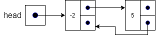
The solution lies in creating our own specialized data structure where each node contains the data of interest as well as a reference, or pointer to the next node in the list. Of course, we would also need to have a pointer to the first node in the list, which we call the head.

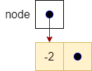
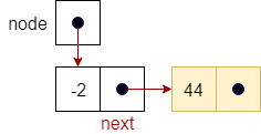
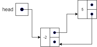
The figure below shows how we can construct a linked list data structure. The head entity shown in the figure is a variable that contains a pointer to the first node in the list, in this case the node containing -2. Each node in the list is an object that has two main parts: the data that it holds, and a pointer to the next item in the list.

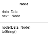
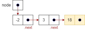
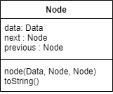
The class representation of a singly linked list Node is shown below. As discussed above, we have two attributes: data, which holds the data of the node, and next, which is a reference or pointer to the next node. We also use a constructor and a standard toString operation to appropriately create a string representation for the data stored in the node.

Linked List

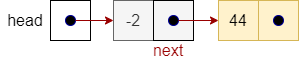
A list is represented by a special variable head that contains a pointer to the first item in the list. If the head is null (equal to 0), then we have an empty list, which is a list with no items in it.

However, if we have items in the list, head will point to a node as shown in the figure below. This node has some data (in this case -2) and its own pointer that points to the next node in the list. As we can see in our example, head points to a sequence of five nodes that makes up our list. The node with the data 67 in it is the last item in the list since its pointer is null. We often refer to this condition as having a null pointer.

While we will not show them explicitly in this module, each pointer is actually an address in memory. If we have a pointer to node X in our node, that means that we actually store the address of X in memory in our node.

Linked List Class

To capture the necessary details for a singly linked list, we put everything into a class. The singly linked list class has two attributes:

• list—the pointer to the first node in the list, and
• size—an integer to keep track of the number of items in the list.

Class SingleLinkedList 
    Node head
    Integer size = 0

While we would normally create getter and setter methods for each attribute in the class, to simplify and clarify our pseudocode below we use “dot notation” to refer directly to the attributes in the node. The following table illustrates our usage in this module.

Use	Meaning
node
node.next
node.next.next
head
head.next

Singly Linked Lists - Insertion

YouTube Video

Given the structure of our linked list, we can easily insert a new node at any location in the list. However, for our purposes we are generally interested in inserting new nodes at the beginning of the list, at some specific location in the list, or in the appropriate order if the list is sorted.

Inserting at the Beginning

Inserting a node at the beginning of a list is straightforward. We just have to be careful about the order we use when swapping pointers. In the prepend code below, line 1 creates the new node to be stored in the list. Next, line 2 assigns the pointer in the new node to point to the pointer held by the head. If there was an item already in the list, head will point to the previous first item in the list. If the list was empty, head will have been null and thus the node.next will become null as well. Line 3 assigns head to point to the new node and line 4 increments our size variable.

function prepend(data)
    node = new Node(data)	(1) 
	node.next = head 	    (2)
	head = node			    (3)
	size = size + 1		    (4)
end function

We show this process in the following example. The figure below shows the initial state as we enter the prepend operation. Our list has three items in it, an “a”, “W”, and “Q” and we want to add the new node “M” in front of item “a”.

The figure below shows the effect of the first step of the operation. This step creates a new node for “M” and changes next to point at the same node as the pointer held by head, which is the address of the first item in the list, “a”.

The result of performing line 3 in the operation is shown below. In line 3 we simply change head to point to our new node, instead of node “a”. Notice now that the new node has been fully inserted into the list.

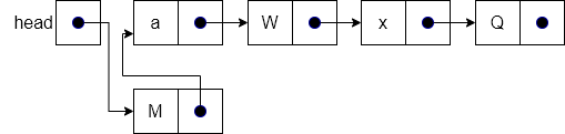
And, if we redraw our diagram a bit, we get a nice neat list!

Since there are no loops in the prepend operation, prepend runs in constant time.

Inserting in the Middle

Inserting a node at a given index in the linked list is a little more difficult than inserting a node at the beginning of the list. First, we have to find the proper location to insert the new node before we can actually insert it. However, since we are given an index number, we simply need to follow the linked list to the appropriate index and then perform the insertion.

We do have a precondition to meet before we proceed, however. We need to make sure that the index provided to the operation is not less than 0 and that it is not greater than the size of the list, which is checked in line 2. If the precondition is not satisfied, we raise an exception in line 3.

function insertAt(data, index)	        (1)
		if index < 0 or index > size	(2)
			raise exception	            (3)
		elseif index == 0	            (4)
			prepend(data)		        (5)
		else
			curr = head.next	        (6)
			prev = head		            (7)
			node = new Node(data)	    (8)
		for i = 1 to index – 1	        (9)
			prev = curr	                (10)
			curr = curr.next	        (11)
		end for			                (12)
		prev.next = node	            (13)
		node.next = curr	            (14)
		size = size + 1	                (15)
	end if
end function

Lines 4 and 5 check to see if the index is 0, which means that we want to insert it as the first item in the list. Since this is the same as the prepend operation we’ve already defined, we simply call that operation. While this may not seem like a big deal, it is actually more efficient and helps us to simplify the code in the rest of the operation.

The operation uses curr to keep track of which node in the list we are currently looking at, thus we initialize curr to point at the first node in the list in line 6. To allow us to swap pointers once we find the appropriate place in the list, we keep track of the node previous to curr as well by using the variable pre. This variable is initialized to head in line 7, and line 8 creates the new node we will insert into our list. After line 8, our list, node, and previous pointers would look like the following (assuming the index passed in was 2).

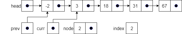
At this point we start our walk through the list using the for loop in lines 9 - 12. Specifically, with an index of 2 we will actually go through the loop exactly one time, from 1 to 1. Each time through the loop, lines 10 and 11 will cause curr and prev to point at the next nodes in the list. At the end of one time through our loop, our example will be as shown below.

Now, the only thing left to do is update the next pointer of node “3” to point at node (line 13), and node.next to point at curr node (line 14), while line 15 increments the size attribute. The updated list is shown below.

The insertAt operation, while being quite flexible and useful, can potentially loop through each node in the list. Therefore, it runs in order $N$ time.

Inserting in Order

When we want to insert an item into an ordered list, we need to find the right place in the list to actually insert the new node. Essentially, we need to search the list to find two adjacent nodes where the first node’s data is less than or equal to data and the second node’s data is greater than data. This process requires a linear search of the list.

function insertOrdered(data) 
		curr = head			                (1)
	index = 0				                (2)
	while curr != NULL AND curr.data < data	(3) 
		index = index + 1	                (4)
		curr = curr.next	                (5)
	end while
	insertAt(data, index)	                (6)
end function

Notice that we do not have a precondition since we will search the list for the appropriate place to insert the new node, even if the list is currently empty. In line 1, we create a curr variable to point to the current node we are checking in the list, while in line 2 we initialize an index variable to keep track of the index of curr in the list.

Next, lines 3 – 5 implement a loop that searches through the list to find a node where the data in that node is greater than or equal to the data we are trying to put into the list. We also check to see if we are at the end of the list. Inside the loop, we increment index and point curr to the next node in the list.

Once we find the appropriate place in the list, we simply call the insertAt operation to perform the actual insertion. Using the insertAt operation provides a nice, easy to understand operation. However, we do suffer a little in efficiency since both operations loop through the list to the location where we want to insert the new data node. However, since the insertAt call is not embedded within the loop, our insertOrdered operation still runs in order $N$ time.

Since the previous example inserts the number 2 into the list (which falls between -1 and 3), the results of running the insertOrdered operation will be the same output as the result of the insertAt operation as shown above.

Singly Linked Lists - Removal

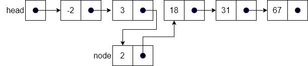
The process of removing a node from a linked list is fairly straightforward. First, we find the node we want to remove from the list and then change the next pointer from the previous node in the list to the next node in the list. This effectively bypasses the node we want to remove. For instance, if we want to remove node “3” from the following list,

we simply change the next pointer in the “-2” node to point to node “18” instead of node “3”. Since no other nodes are pointing at node “3” it is effectively removed from our list as shown below. We then return the data in that node to the requesting function. Eventually, the garbage collector will come along and realize that nothing is referencing node “3” and put it back into available memory.

Removing at the Beginning

Removing an item at the beginning of a list is extremely simple. After checking our precondition in line 1, which ensures that the list is not empty, we create a temporary copy of the data in the first node in line 3 so we can return it later in line 6. However, the actual removal of the first node simply requires us to point head to the second node in the list (line 4), which is found at head.next. This effectively skips over the first node in the list. Finally, we decrement our size variable in line 5 to keep it consistent with the number of nodes now in the list. Since there are no loops, removeFirst runs in constant time.

function removeFirst() returns data
		if size == 0			(1)
			raise exception	    (2)
		end if
		temp = head.data		(3)
	head = head.next 	        (4)
	size = size – 1		        (5)
	return temp			        (6)
end function

Removing in the Middle

Removing a node at a specific index in the list is more difficult than simply removing the first node in the list since we have to walk through the list to find the node we want to remove before we can actually remove it. In addition, while walking through the list, we must keep track of the current node as well as the previous node, since removing a node requires us to change the previous node in the list.

In our removeAt operation below, we first check our precondition in line 1 to ensure that the index provided is a valid index in the list. If it is, we check to see if index is 0 in line 3 and call the removeFirst operation in line 4 if it is.

function removeAt(index) returns data
    if index < 0 OR index > size – 1	(1)
        raise exception	                (2)
    else if index == 0	                (3)
        return removeFirst()            (4)
    else
        curr = head.next	            (5)
        prev = head		                (6)

        for i = 1 to index - 1 	        (7)
            prev = curr	                (8)
            curr = curr.next	        (9)
        end for
        prev.next = curr.next	        (10)
        size = size – 1	                (11)
        return curr.data	            (12)
    end if
end function

Before we start our walk through the list using the for loop in lines 7 - 9, we declare two variables in lines 5 and 6:

• curr points to the current node in our walk, and
• prev points to the node before curr in the list.

Lines 7 – 9 are the for loop that we use to walk through the list to find the node at index. We simply update the values of prev and curr each time through the loop to point to the next node in the list.

Once we complete the for loop, curr is pointing at the node we want to remove and prev points at the previous node. Thus, we simply set prev.next = curr.next to bypass the curr node, decrement our size attribute by 1 to retain consistency, and return the data associated with the curr node.

Like the insertAt operation, the removeAt operation uses a loop and thus runs in order $N$ time.

Removing Instances of a Node

If we want to remove all occurrences of a specific node from the list, we take the data we want to remove from the list and then search all nodes in the list, removing any whose data matches the data from the input node. We will return the number of nodes removed from the list.

function removeData(data)
	curr = head			            (1)
	index = 0				        (2)
	while (curr != null) 	        (3)
		if (curr.data == data) 	    (4)
			removeAt(index)	        (5)
		end if
		index = index + 1	        (6)
		curr = curr.next	        (7)
	end while	
end function

To simplify this operation, we will call the removeAt operation to actually remove the node from the list, leaving this operation to simply find the nodes whose data match the input data. We will use two variables in this operation:

• curr will point to the current node we are checking, and
• index will keep track of the index of the curr node so we can use the removeAt operation.

The main part of the operation is a while loop (lines 3 – 7) that walks through the list, node by node. For each node in the list, we check if its data matches the input data in line 5, and then call removeAt to remove it from the list if it does. Then, each time through the loop, we increment index in line 7 and then point curr to the next node in the list in line 8. When our loop exits, we have removed all the nodes whose data matched the input data.

Since we walk through the entire list, the removeData operation runs in order $N$ time.

Singly Linked Lists - Other Operations

isEmpty

The list isEmpty operation is rather straightforward. We simply need to return the truth of whether head.next has a null pointer. Obviously, isEmpty runs in constant time.

function isEmpty() returns boolean
    return head == NULL       (1)
end function

peek

The peek operation is designed to return the data from the last node inserted into the list, which is the node pointed at by head. This is easy to do; however, we must ensure that we check to see if the list is empty in line 1 before we return the head.data in line 3. Due to its simple structure, the run time of the peek operation is constant.

function peek() returns data
	if isEmpty()			(1)
		raise exception		(2)
	end if
	return head.data		(3)
end function

peekEnd

The peekEnd operation is designed to return the first node inserted into the list, which is now the last node in the list. Like the peek operation, we must ensure the list is not empty in line 1 before actually searching for the end of the list. Lines 3 – 5 walk through the list using a while statement until curr.next is null, signifying that curr is pointing at the last node in the queue. Finally, line 6 simply returns the data in the last node. Since peekEnd must walk through the entire list to find the last node, it runs in order $N$ time.

function peekEnd() returns data
	if isEmpty()			    (1)
		raise exception		    (2)
	end if
    curr = head 			    (3)
    while curr.next != null		(4)
        curr = curr.next		(5)
    end while
    return curr.data			(6)
end function

List-Based Stacks

YouTube Video

If we implement a stack using a singly linked list, we can simplify many things about the implementation. First of all, we can totally remove the isFull, doubleCapacity, and halveCapacity operations since we can grow and shrink our list-based stack as needed. The rest of the operations can be implemented directly with list operations. The front of the list will be the top of the stack since the operations to insert and remove items from the front of list are very efficient.

To implement our stack, we assume we have declared a linked list object named list.

Push

As expected, the push operation is almost trivial. We simply call the list prepend operation to insert the data into the front of the list.

function push(data)
	list.prepend(data)
end function

Pop

Like push, the pop operation is also easily implemented using the removeFirst operation of our linked list. As long as the list is not empty, we simply return the data from the first item when we remove it from the list.

function pop() returns data
	if list.isEmpty() then
		throw exception
	end if
    return list.removeFirst().data
end function

isEmpty

The isEmpty operation is even easier. It is implemented by simply returning the results of the list isEmpty operation.

function isEmpty() return boolean
	return list.isEmpty()
end function

Peek

The stack peek operation is also straightforward. To implement the peek operation we simply return the results from the list peek operation, which returns the data from the first node in the list.

function peek() returns data
    return list.peek()
end function

As we can see, each of the major operations for a stack is implemented easily using list operations that run in constant time. This makes list-based stacks extremely efficient data structures to use.

Doubly Linked Lists

YouTube Video

With singly linked lists, each node in the list had a pointer to the next node in the list. This structure allowed us to grow and shrink the list as needed and gave us the ability to insert and delete nodes at the front, middle, or end of the list. However, we often had to use two pointers when manipulating the list to allow us to access the previous node in the list as well as the current node. One way to solve this problem and make our list even more flexible is to allow a node to point at both the previous node in the list as well as the next node in the list. We call this a doubly linked list.

The concept of a doubly linked list is shown below. Here, each node in the list has a link to the next node and a link to the previous node. If there is no previous or next node, we set the pointers to null.

Doubly Linked Node

A doubly linked list node is the same as a singly linked list node with the addition of the previous attribute that points to the previous node in the list as shown below.

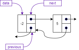
The class representation of a doubly linked list Node is shown below. As discussed above, we have three attributes:

• data, which holds the data of the node,
• next, which is a pointer to the next node, and
• previous, which is a pointer to the previous node.

We also use a constructor and the standard toString operation to create a string for the data stored in the node.

Doubly Linked List

As with our singly linked list, we start off a doubly linked list with a pointer to the first node in the list, which we call head. However, if we also store the pointer to the last node in the list, we can simplify some of our insertion and removal operations as well as reduce the time complexity of operations that insert, remove, or peek at the last node in the list.

The figure below shows a doubly linked list with five nodes. The variable head points to the first node in the list, while the variable tail points to the last node in the list. Each node in the list now has two pointers, next and previous, which point to the appropriate node in the list. Notice that the first node’s previous pointer is null, while the last node’s next pointer is also null.

Doubly Linked List Class

Like we did for our singly linked list, we capture the necessary details for our doubly linked list in a class. The doubly linked list class has four attributes:

• head—the pointer to the first node in the list,
• tail—the pointer to the last node in the list,
• current—the pointer to the current node used by the iterator, and
• size—an integer to keep track of the number of items in the list.

Class DoubleLinkedList 
    Node head
    Node tail
    Node current
    Integer size = 0

Doubly Linked Lists - Insertion

Insertion in doubly linked lists is similar to what we saw in the singly linked list with two exceptions:

1. We must update both the previous and next pointers in all affected nodes.
2. We can use the tail pointer to make the insertion of data at the end of the list very efficient.

Inserting at the Beginning

Inserting at the beginning of a doubly linked list is almost as straightforward as in a singly linked list. We just need to make sure that we update the previous pointer in each affected node. After creating the new node in line 1, we check to see if the list is empty in line 2. If it is empty, then we only have to worry about updating the head and tail pointers to both point at node in lines 3 and 4. If the list is not empty, we have the situation shown below.

To insert a node at the beginning of the list, we set head.previous (the previous pointer in the first node in the list) to point to the new node in line 5.

Next, we set the next pointer in the new node to point to where head is currently pointing in line 6, which is the first node in the list.

Finally, we update head to point to the new node and then increment the size in line 8.

With a little bit of reformatting, we can see that we’ve successfully inserted our new node in the list.

The pseudocode for this operation is given below.

function prepend(data)
	node = new Node(data)	    (1)
	if size == 0	            (2)
		head = node	            (3)
		tail = node	            (4)
	else
		head.previous = node	(5)
		node.next = head	    (6)
		head = node	            (7)
	end 
	size = size + 1	            (8)
end function

Since there are no loops in the prepend code, the code runs in constant time.

Inserting in the Middle

Inserting a new node at some arbitrary index in a doubly linked list is similar to the same operation in a singly linked list with a couple of changes.

1. If the index is at the end of the list, we can use an efficient append operation (defined below) to insert the node at the end of the list.
2. When walking through the list to the correct index, we do not need to keep track of the previous node.
3. We will have to update both the previous and next pointers in all affected nodes.

Lines 1 and 2 in the code check to ensure that the index is a valid number, then we check to see if we are inserting at the beginning or end of the list in lines 2 and 4. If we are, we simply call the appropriate method, either prepend or append.

If none of those conditions exist, then we start the process of walking through the list to find the node at index. To do this, we need to create the new node we want to insert and then create a temporary pointer curr that we will use to point to the current node on our walk.

Lines 10 and 11 form the loop that walks through the list until we get to the desired index. When the loop ends, we will want to insert the new node between curr and curr.next. Thus, we set the appropriate values for the new node’s next and previous pointers in line 12 and 13. Then, we set the previous pointer in node.next to point back to node in line 14 and then set curr.next to point at the new node. Finally, we increment size by 1.

function insertAt(data, index)
	if index < 0 OR index > size	(1)
		raise exception	            (2)
	else if index == 0	            (3)
		prepend(data)	            (4)
	else if index == size	        (5)
		append(data)	            (6)
	else				            (7)
		node = new node(data)	    (8)
		curr = head	                (9)

		for i = 1 to index -1	    (10)
			curr = curr.next	    (11)
		end for

		node.next = curr.next	    (12) 
		node.previous = curr	    (13)
		node.next.previous = node	(14)
		curr.next = node	        (15)
		size = size + 1	            (16)
	end if
end function

Although prepend and append run in constant time, the general case will cause us to walk through the list using a for loop. Therefore, the insertAt operation runs in order $N$ time.

Inserting at the End

Since we have added the tail pointer to the doubly linked list class, we can make adding a node at the end of the list run in constant time instead of order $N$ time. In fact, if you look at the code below for the append operation, it is exactly the same as the constant time prepend operation except we have replaced the head pointer with the tail pointer in lines 5 – 7.

function append(data)
	node = new node(data)	     (1)
	if size == 0	             (2)
		tail = node	             (3)
		head = node	             (4)
	else
		tail.next = node	     (5)
		node.previous = tail 	 (6)
		tail = node	             (7)
	end if
	size = size + 1	             (8)
end function

Doubly Linked Lists - Removal and Peek

The process of removing a node from a doubly linked list is really no more difficult than from a singly linked list. The only difference is that instead of changing just one pointer, we now also need to modify the previous pointer in the node following the node we want to remove. For instance, if we want to remove node “3” from the following list,

we simply modify the next pointer in node “-2” to point to node “23”. Then, we modify the previous pointer in node “23” to point to node “-2”. We then return the data in that node to the requesting function.

Removing at the Beginning

The remove operation removes the first node in the list. First, we check to ensure that there is at least one node in the list in line 1 and raise an exception if there is not. Now, the process is simple. We simply create a temporary pointer temp that points to the node we are going to delete in line 3 and then point head to head.next, which is the second node in the list. Then, in line 5, we check to see if the list is empty (head == null) and set tail to null if it is (it was pointing at the node we just removed). If the list is not empty, we do not need to worry about updating tail; however, we do need to set the previous pointer of the first node in the list to null (it was also pointing at the node we just removed). Finally, we decrement size in line 8 and then return the data in the node we just removed in line 9. Obviously, the operation runs in constant time since there are no loops.

function remove() returns data
	if size == 0	            (1)
		raise exception	        (2)
	end if
	temp = head		            (3)
	head = head.next	        (4)
	if head == null	            (5)
		tail = null	            (6)
	else
		head.previous = null	(7)
	end if
	size = size – 1	            (8)
	return temp.data	        (9)
end function

Removing in the Middle

Removing a node at a specific index is very similar to the way we did it in singly linked lists. First, if we have an invalid index number, we raise an exception in line 2. Otherwise we check for the special cases of removing the first or last node in the list and calling the appropriate operations in lines 3 – 6. If we have no special conditions, we create a temporary pointer curr and then walk through our list in lines 7 – 9. Once we reach the node we want to remove, we simply update the next node’s previous pointer (line 10) and the previous node’s next pointer (line 11) and we have effectively removed the node from the list. We then decrement size in line 12 and return the data from the removed node in line 13.

Since the operation relies on a loop to walk through the list, the operation runs in order $N$ time.

function removeAt(index) returns data
	if index < 0 OR index > size – 1	    (1)
		raise exception	                    (2)
	else if (index == 0)	                (3)
		return remove()	                    (4)
	else if index == size – 1	            (5)
		return removeLast()	                (6)
	else	
		curr = head.next;	                (7)
        for i = 1 to index -1 	            (8)
            curr = curr.next	            (9)
        end for

        curr.next.previous = curr.previous	(10)
        curr.previous.next = curr.next	    (11)
        size = size – 1	                    (12)
        return curr.data	                (13)
    end if
end function

Removing at the End

Since we have added the tail pointer to the doubly linked list class, we can make removing a node at the end of the list run in constant time instead of running in order $N$ time. In fact, if you look at the code below for the removeLast operation, it is almost exactly the same as the constant time removeFirst operation. The only difference is that we have replaced the head pointer with the tail pointer and head.next with tail.previous in lines 3 – 7.

function removeLast() returns data
	if size == 0	        (1)
		raise exception	    (2)
	end if	
	temp = tail		        (3)
	tail = tail.previous	(4)
	if tail == null	        (5)
		head = null	        (6)
	else	
		tail.next = null	(7)
	end if
	size = size – 1	        (8)
	return temp.data	    (9)
end function

PeekEnd

Another operation impacted by the addition of the tail pointer is the peekEnd operation. Since we can access the last node in the list directly, we just need to make sure that the list is not empty, which we do in lines 1 and 2. Then, we can return the tail.data.

function peekEnd() returns data
	if isEmpty()	        (1)
		raise exception 	(2)
	else	
		return tail.data	(3)
	end if
end function

List Iterators

YouTube Video

An iterator is a set of operations a data structure provides to allow users to access the items in the data structure sequentially, without requiring them to know its underlying representation. There are many reasons users might want to access the data in a list. For instance, users may want to make a copy of their list or count the number of times a piece of data was stored in the list. Or, the user might want to delete all data from a list that matches a certain specification. All of these can be handled by the user using an iterator.

At a minimum, iterators have two operations: reset and getNext. Both of these operations use the list class’s current attribute to keep track of the iterator’s current node.

Reset

The reset operation initializes or reinitializes the current pointer. It is typically used to ensure that the iterator starts at the beginning of the list. All that is required is for the current attribute be set to null.

function reset()
	current = null
end function

Get Next

The main operation of the iterator is the getNext operation. Basically, the getNext operation returns the next available node in the list if one is available. It returns null if the list is empty or if current is pointing at the last node in the list.

Lines 1 and 2 in the getNext operation check to see if we have an empty list, which results in returning the null value. If we have something in the list but current is null, this indicates that the reset operation has just been executed and we should return the data in the first node. Therefore, we set current = head in line 4. Otherwise, we set the current pointer to point to the next node in the list in line 5.

function getNext() returns data
	if isEmpty()	            (1)
		return null	            (2)
	end if 
	if current == null	        (3)
		current = head	        (4)
	else
		current = current.next	(5)
	end if
	if current == null	        (6)
		return null	            (7)
	else
		return current.data	    (8)
	end if
end function

Next we return the appropriate data. If current == null we are at the end of the list and so we return the null value in line 7. If current is not equal to null, then it is pointing at a node in the list, so we simply return current.data in line 8.

Remove current

While not technically part of the basic iterator interface, the removeCurrent operation is an example of operations that can be provided to work hand-in-hand with a list iterator. The removeCurrent operation allows the user to utilize the iterator operations to find a specific piece of data in the list and then remove that data from the list. Other operations that might be provided include being able to replace the data in the current node, or even insert a new piece of data before or after the current node.

The removeCurrent operation starts by checking to make sure that current is really pointing at a node. If it is not, then the condition is caught in line 1 and an exception is raised in line 2. Next, we set the next pointer in the previous node to point to the current node’s next pointer in lines 3 – 5, taking into account whether the current node is the first node in the list. After that, we set the next node’s previous pointer to point back at the previous node in line 6 – 8, considering whether the node is the last node in the list. Finally, we decrement size in line 9.

function removeCurrent()
	if current == null		                        (1)
		raise exception	                            (2)
	end if 
	if current.previous != null	                    (3)
		current.previous.next = current.next	    (4)
	else
		head = current.next	                        (5)
	end
	if current.next != null	                        (6)
		current.next.previous = current.previous	(7)
	else
		tail = current.previous	                    (8)
	end if
    current = current.previous                      (9)
	size – size – 1	                                (10)
end function

Using an Iterator

There are several applications for list iterators. For our example, we will use the case where we need a function to delete all instances of data in the list that match a given piece of data. Our deleteAll function resides outside the list class, so we will have to pass in the list we want to delete the data from. We start the operation by initializing the list iterator in line 1, followed by getting the first piece of data in the list in line 2. Next, we’ll enter a while loop and stay in that loop as long as our copy of the current node in the list, listData, is not null. When it becomes null, we are at the end of the list and we can exit the loop and the function.

function deleteAll(list, data)
	list.reset()	                (1)
	listData = list.getNext()	    (2)
	while listData != null	        (3)
		if listData == data	        (4)
			list.removeCurrent()	(5)
		end if	
		listData = list.getNext()	(6)
	end while
end function

Once in the list, it’s a matter of checking if our listData is equal to the data we are trying to match. If it is, we call the list’s removeCurrent operation. Then, at the bottom of the list, we get the next piece of data from the list using the list iterator’s getNext operation.

By using a list iterator and a limited set of operations on the current data in the list, we can allow list users to manipulate the list while ensuring that the integrity of the list remains intact. Since we do not know ahead of time how a list will be used in a given application, an iterator with associated operations can allow the user to use the list in application-specific ways without having to add new operations to the list data structure.

List-Based Queues

YouTube Video

Implementing a queue with a doubly linked list is straightforward and efficient. The core queue operations (enqueue, dequeue, isEmpty, and peek) can all be implemented by directly calling list operations that run in constant time. The only other major operation is the toString operation, which is also implemented by directly calling the list toString operation; however, it runs in order $N$ time due to the fact that the list toString operation must iterate through each item in the list.

The key queue operations and their list-based implementations are shown below.

function enqueue (data)
    list.append(data)
end function

function dequeue() returns data
    return removeFirst()
end function

function isEmpty() returns Boolean
    return list.isEmpty()
end function

function peek() returns data
    return list.peek()
end function

function toString() returns data
    return list.toString()
end function

Lists Summary

In this module, we introduced the concept of a linked list, discussing both singly and doubly linked lists. Both kinds of lists are made up of nodes that hold data as well as references (also known as pointers) to other nodes in the list. Singly linked lists use only a single pointer, next, to connect each node to the next node in the list. While simple, we saw that a singly linked list allowed us to efficiently implement a stack without any artificial bounds on the number of items in the list.

With doubly linked lists, we added a previous pointer that points to the previous node. This makes the list more flexible and makes it easier to insert and remove nodes from the list. We also added a tail pointer to the class, which keeps track of the last node in the list. The tail pointer significantly increased the efficiency of working with nodes at the end of the list. Adding the tail pointer allowed us to implement all the major queue operations in constant time.