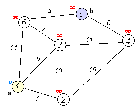
CC 310 Textbook
This is the homepage
This is the homepage
Welcome to CC 310!
Hello and welcome to the Computational Core program!
My name is Russ Feldhausen, and I’ll be one of the instructors for this program. My contact information is shown here, and is also listed on the syllabus
[Slide 2]
There are many other instructors and TAs for this program that you may interact with or see in the tutorial videos. They all have been instrumental in the development of this program. Specifically, I’d like to recognize the work of Nathan Bean, the developer of the CIS 400 course on which this course is based.
[Slide 3]
In this course we will primarily use a KSU email group (cc410-help or cc410-help@ksuemailprod.onmicrosoft.com) to communicate. Email sent to this address is forwarded to all instructors and TAs. Our replies to you will also be shared amongst the instructors and TAs so we all have access to the assistance you have already received. We will respond to you within a business day, so be aware that a question emailed Friday night may not receive an answer before Monday. Please read and adhere to the guidance on Netiquette in the syllabus for all electronic communications.
[Slide 3]
In addition to email and Canvas, we’ll be using the online learning platform Codio for most of the programming tutorials and projects in this program. We’ll also discuss how to use Codio later in this module.
[Slide 5]
The Computational Core program consists of several courses, and each course contains a number of learning modules. In general, there are about 12-15 modules per course. Each module will usually consist of an interactive tutorial using Codio, followed by a quiz through Canvas, and lastly a programming project in Codio. In CC 410, there will also be several guided examples for you to follow and submit. The modules themselves are gated, which means that you much complete each item in the module before continuing. In addition, the modules enforce prerequisite requirements from other modules. For CC 410 you must complete them in order starting with module 0.
You are welcome to work on this course at any time during the week as your schedule allows, provided that you complete each module before the listed due date. There will be roughly one module due each week. Unlike other Computational Core courses, CC 410 does not include many auto-graded assignments. This is primarily due to the open-ended nature of the course. Instead, your code will be reviewed by an instructor or TA and you’ll receive feedback through Canvas and Codio. In some instances, you may be encouraged to redo parts of an assignment for additional credit. We will strive to provide feedback on an assignment within one week of it being submitted.
[Slide 6]
Looking ahead to the rest of this introductory module, you’ll see that there are a few more items to be completed before you can move on. In the next video, I’ll discuss a bit more information about navigating through this course on Canvas and using the Codio learning environment.
[Slide 7]
One thing I highly encourage each of you to do is read the syllabus for this course in its entirety, and let us know if you have any questions. My view is that the syllabus is a contract between me as your teacher and you as a student, defining how each of us should treat each other and what we should expect from each other. We have made a few changes to the standard syllabus template for this program, and those changes are clearly highlighted. Finally, the syllabus itself is subject to change as needed as we adapt this program to meet the needs of its students, and all changes will be clearly communicated to everyone before they take effect.
[Slide 8]
One very important part of the syllabus that every student should read is the late work policy. First off, each module has a due date, and you may work on that module at any time before it is due, provided you have met the prerequisites. As discussed before, you must do all the readings and assignments in a module, preferably in listed order, before moving on, so you cannot jump ahead. A module is considered completed when all items have been completed.
[Slide 9]
For the purposes of grading, we will use the date and time that the confirmation quiz was submitted at the end of each module to determine when the module was completed. This is due to the way that Codio handles grading, as it may resubmit previously graded assignments if an error in the module is corrected, making a previously completed assignment appear to be submitted late.
If a module is completed after the due date, a penalty of 10% of the total points of each assignment will be deducted for each day the assignment is late. Therefore, if an assignment is submitted 3 days late, it will be subject to a 30% penalty of the total number of points possible on that assignment. After 10 days, no points will be awarded for a late submission.
However, even if a module is late, it still must be completed before you can move on to a later module. So, it is very important to avoid getting behind in this course, as it can be very difficult to get back on track. If you ever find that you are struggling to keep up, please don’t be afraid to contact either the instructors or GTAs for assistance. We’d be happy to help you get caught back up quickly.
The grading in this course is very simple. First, 10% of your final grade will depend on the grades you receive from each of the tutorials and quizzes throughout the course. Next, 10% of your grade will come from the interactive examples that precede several projects. The next 40% of your grade will come from the numerous project milestones throughout the course, of which there will be approximately 10. There will also be a couple of “concept quizzes” throughout the semester, which are a bit longer than a normal quiz and will ask you to apply what you’ve learned to a novel situation. Those are worth 15% of your grade. Finally, the last 25% of your grade will come from the final project in the course, which will be discussed in a later video. In this program, the standard “90-80-70-60” grading scale will apply, though I reserve the right to curve grades up to a higher grade level at my discretion. Therefore, you will never be required to get higher than 90% for an A, but you may get an A if you score slightly below 90% if I choose to curve the grades.
[Slide 10]
This is intended to be a completely online, self-paced course. There are no mandatory scheduled course times. All of the content is available online, so you can work whenever and wherever you want. It could be a 3-hour block once a week, or a few minutes here and there between classes. It’s really up to you and your schedule. However, remember that each module may require 12 to 16 or more hours of work to complete, so make sure you have plenty of time available to devote to this course.
In addition, due to the flexible online format of this class, there won’t be any long lecture videos to watch. Instead, each module will consist of a guided tutorial and several short videos, each focused on a particular topic or task. Likewise, there won’t be any textbooks required, since all of the information will be presented in the interactive tutorials through Codio. Finally, since we are using Codio as our learning platform, you won’t have to deal with installing and using a clunky integrated development environment, or IDE, just to learn how to program. Codio helps make learning to program quick and painless by moving everything to the web.
[Slide 11]
What hasn’t changed, though, is the basic concept of a college course. You’ll still be expected to watch or read about 6-9 hours of content to complete each module. In addition to that, each project assignment may require another 6-9 hours of work to complete. If you plan on doing a module each week, that roughly equates to 6 hours of content and 6 hours of homework each week, which is the expected workload from a 3-4 credit hour college course.
From my experience, I can definitely share that the number one reason students struggle in this class is due to poor time management, not the complexity of the material. So, make sure you are planning to dedicate enough time to this course, and strive to start assignments as soon as you receive them so you have lots of time to get help if you get stuck.
[Slide 12]
For this course, the only supplies you’ll need as a student are access to a modern web browser and a broadband internet connection. No other special hardware or software is necessary! However, in this course you will also be able to do some development on your own computer using Visual Studio Code and Ubuntu. We’ll provide some short videos to help you get started if you choose to go that route, but it is not required. Due to the complex nature of this course, we do not recommend using phones, tablets, or Chromebooks if you choose to do development on your own systems.
[Slide 13]
Finally, as you are aware, this course is always subject to change. This is a relatively new program here at K-State, and we’re always working on new and interesting ideas to integrate into the courses. The best advice I have is to look upon this graphic with the words “Don’t Panic” written in large, friendly letters. If you find yourself falling behind, or not understanding seek our help via cc410-help.
[Slide 14]
So, to complete this module, there are a few other things that you’ll need to do. The next step is to watch the video on navigating Canvas and Codio, which will give you a good idea of how to most effectively work through the content in this course.
[Slide 15]
To get to that video, click the “Next” button at the bottom right of this page.
This course makes extensive use of several features of Canvas which you may or may not have worked with before. To give you the best experience in this course, this video will briefly describe those features and the best way to access them.
When you first access the course on Canvas, you will be shown this homepage. It contains quick links to the course syllabus and Piazza discussion boards. This is handy if you just need to jump to a particular area.
Let’s walk through the options in the main menu to the left. The first section is Modules, which is where you’ll primarily interact with the course. You’ll notice that I’ve disabled several of the common menu items in this course, such as Files and Assignments. This is to simplify things for you as students, so you remember that all the course content is available in one place.
When you first arrive at the Modules section, you’ll see all of the content in the course laid out in order. If you like, you can minimize the modules you aren’t working on by clicking the arrow to the left of the module name. I’ll do so, leaving the introductory module open.
As you look at each module, you’ll see that it gives quite a bit of information about the course. At the top of each module is an item telling you what parts of the module you must complete to continue. In this case, it says “Complete All Items.” Likewise, the following modules may list a number of prerequisite modules, which you must complete before you can access it.
Within each module is a set of items, which must be completed in listed order. Under each item you’ll see information about what you must do in order to complete that item. For many of them, it will simply say view, which means you must view the item at least once to continue. Others may say contribute, submit, or give a minimum score required to continue. For assignments, it also helpfully gives the number of points available, and the due date.
Let’s click on the first item, Course Introduction, to get started. You’ve already been to this page by this point. Many course pages will consist of an embedded video, followed by links to any resources used or referenced in the video, including the slides and a downloadable version of the video. Finally, a rough video script will be posted on the page for your quick reference.
While I cannot force you to watch each video in its entirety, I highly recommend doing so. The script on the page may not accurately reflect all of the content in the video, nor can it show how to perform some tasks which are purely visual.
When you are ready to move to the next step in a module, click the Next button at the bottom of the page. Canvas will automatically add Next and Previous buttons to each piece of content which is accessed through the Modules section, which makes it very easy to work through the course content. I’ll click through a couple of items here.
At any point, you may click on the Modules link in the menu to the left to return to the Modules section of the site. You’ll notice that I’ve viewed the first few items in the first module, so I can access more items here. This is handy if you want to go back and review the content you’ve already seen, or if you leave and want to resume where you left off. Canvas will put green checkmarks to the right of items you’ve completed.
Continuing down the menu to the left, you’ll find the usual Canvas links to view your grades in the course, as well as a list of fellow students taking the course.
===
Now, let’s go back to Canvas and load up one of the Codio projects. To load the first Codio projects, click the Next button at the bottom of this page to go to the next part of this module, which is the Codio Introduction tutorial. On that page, there will be a button to click, which opens Codio in a new browser window or tab.
Once Codio loads, it should give you the option to start the Guide for that module. You’ll definitely want to select that option whenever you load a Codio project for the first time.
From there, you can follow the steps in that guide to learn more about the Codio interface. The first page of the guide continues this video. I’ll see you there!
As you work on the materials in this course, you may run into questions or problems and need assistance. This video reviews the various types of help available to you in this course.
First and foremost, anytime you have a questions or need assistance in the Computational Core program, please send an email to the appropriate help group for this course. In this case, it would be cc410-help, or cc410-help@ksuemailprod.onmicrosoft.com. That email goes to the instructors and GTAs, and is your best chance to get a quick response. We’ll respond to your email within one business day.
Beyond email, there are a few resources you should be aware of. First, if you have any issues working with K-State Canvas, K-State IT resources, or any other technology related to the delivery of the course, your first source of help is the K-State IT Helpdesk. They can easily be reached via email at helpdesk@ksu.edu. Beyond them, there are many online resources for using Canvas, all of which are linked in the resources section below the video. As a last resort, you may also want to email the help group, but in most cases we may simply redirect you to the K-State helpdesk for assistance.
Similarly, if you have any issues using the Codio platform, you are welcome to refer to their online documentation. Their support staff offers a quick and easy chat interface where you can ask questions and get feedback within a few minutes.
If you have issues with the technical content of the course, specifically related to completing the tutorials and projects, there are several resources available to you. First and foremost, make sure you consult the vast amount of material available in the course modules, including the links to resources. Usually, most answers you need can be found there.
If you are still stuck or unsure of where to go, the next best thing is to post your question as an email to the help group. As discussed earlier, the instructors and GTAs will do their best to help you as soon as they can.
Of course, as another step you can always exercise your information-gathering skills and use online search tools such as Google to answer your question. While you are not allowed to search online for direct solutions to assignments or projects, you are more than welcome to use Google to access programming resources such as StackOverflow, language documentation, and other tutorials. I can definitely assure you that programmers working in industry are often using Google and other online resources to solve problems, so there is no reason why you shouldn’t start building that skill now.
Next, we have grading and administrative issues. This could include problems or mistakes in the grade you received on a project, missing course resources, or any concerns you have regarding the course and the conduct of myself and your peers. Since this is an online course, you’ll be interacting with us on a variety of online platforms, and sometimes things happen that are inappropriate or offensive. There are lots of resources at K-State to help you with those situations. First and foremost, please email me directly as soon as possible and let me know about your concern, if it is appropriate for me to be involved. If not, or if you’d rather talk with someone other than me about your issue, I encourage you to contact either your academic advisor, the CS department staff, College of Engineering Student Services, or the K-State Office of Student Life. Finally, if you have any concerns that you feel should be reported to K-State, you can do so at https://www.k-state.edu/report/. That site also has links to a large number of resources at K-State that you can use when you need help.
Finally, if you find any errors or omissions in the course content, or have suggestions for additional resources to include in the course, email the help group. There are some extra credit points available for helping to improve the course, so be on the lookout for anything that you feel could be changed or improved.
So, in summary, reviewing the existing course content should always be your first stop when you have a question or run into a problem, since most issues can be solved there. If you are still stuck, email cc410-help to ask for assistance, and we’ll get back to you within a business day. For issues with Canvas or Codio, you are also welcome to refer directly to the resources for those platforms. For grading questions and errors in the course content or any other issues, please email cc410-help or the instructors directly for assistance.
Our goal in this program is to make sure that you have the resources available to you to be successful. Please don’t be afraid to take advantage of them and ask questions whenever you want.
Before we launch into the course itself, I wanted to take a few minutes to share some information with you regarding what we know about how students learn to program. This isn’t just anecdotal evidence from computer science teachers like me, but theories and research from education researchers who study how humans learn new skills and abilities throughout their lives.If I had to summarize all of this information in as few words as possible, I’d simply say “do the work.” Learning to program is difficult, and the only way to really get good at it is through constant practice and learning. However, that greatly oversimplifies the information that I want to share, and I’m hoping that you’ll find some helpful takeaways from this video that you can incorporate into your learning process.
Before I begin, I want go give all the credit to Nathan Bean for developing this information as part of his CIS 400 course. He graciously allowed me to use his hard work here, and I encourage you to check out his original version, which is available at the URL shown on this slide.
The statement “do the work” is a shorter version of a very common quote from educators, which is “the person doing the work is the person doing the learning.” I couldn’t find a solid reference for who said it first, so I’ll just attributed it to various educators throughout time. This really highlights one of the biggest struggles many students run into when learning to program. There are so many guides online, and the answer to many simple problems can be found through a quick Google search. You can just copy and paste the code, and then your program works. However, did you really learn how to write that program and what it does, or just how to find a quick answer? While this may be a useful tactic from time to time, if you rely too much on other people to do your coding, you really won’t learn it yourself. This is just like learning to shoot free throws on a basketball court or beating your best time in a speedrun - you can’t just watch someone do it and expect to do it yourself (believe me, I’ve tried). So, if you aren’t doing the work, you aren’t really learning.
Next, let’s address a major myth in computer science. I’ve heard this many times: “some people are just natural born programmers, and others simply cannot learn to program.” And yes, on the surface, it may appear to be this way. Some students just seem to have a knack for programming, and you may sit and struggle and not really get anywhere. However, there is no innate skill or ability that makes you good at programming.
Instead, let’s reframe what it means to learn programming. At its core, programming is learning to write steps to solve problems in a way that a computer can perform those steps. That’s really what we are doing when we learn programming.
So, we must focus on learning how to write those steps with the proper exactitude and precision so that they make sense, and we must understand how a computer functions to be able to program that computer effectively. So, when you see someone who is good at programming, it’s not because they are good at some esoteric skill that you’ll never have - they just know how to express their steps properly and know enough about how a computer works to make their program do what they want. That’s really it! And, to be honest, after a single semester of learning to program, you’ll have all the skills you need to do both of those things! If you know how to make conditionals, loops, functions, and use simple variables and arrays, that’s really all you need. Everything else that comes after that is just refining those skills to make your programs more powerful and your coding more efficient.
So, how do we learn these skills? Well, there are a couple of important pieces we need to make sure are in the right place first. For starters, we need to have the correct mindset. Many times I’ll see students struggle to learn how to program, and they’ll say things like what you see on this slide. “Its too hard.” “I don’t understand this.” “I give up.” Statements like this are the sign of a “fixed mindset,” and they can be one of the greatest blockers preventing you from really learning to program. Just like learning any other skill, you have to be open to instruction and willing to learn, or else you’ve failed before you even started.
Instead, we want to focus on building a growth mindset. In the TED talk by Carol Dweck that is linked below this video, which I encourage you to watch, she talks about the power of “yet.” We can turn these statements around by simply adding positive power of “yet” - “I don’t understand this yet.” “I love a good challenge.” “I’ll keep trying until I get it.” Going into a programming project with a mindset that is open to growth and change is really an important first steps. When I feel like I’m getting a fixed mindset, I like to think about how difficult it would be to teach a child to tie their shoes if they don’t want to learn. As soon as I realize that, it is pretty easy to recognize that same problem in myself and work to correct it.
So, once we have our growth mindset, how do we actually learn to program? To understand that, let’s dive a bit into the world of educational theory and the work of Jean Piaget. Piaget was a biologist and psychologist who studied how young children acquired new knowledge, and he helped pioneer the concept of Constructivism, one of the most influential philosophies in education. You can read more about Constructivism in the links below this video.
One particular thing that Piaget worked on was a theory of genetic epistemology. Epistemology is the term for the study of human knowledge, so genetic epistemology is the study of the origins, or genesis, of that knowledge. Put more clearly, it’s the study of how humans create new knowledge. This concept was inspired by research done on snails - he was able to prove that two previously distinct species of snails were actually the same by moving snails from one habitat to another and observing how they modified their behaviors and how their shells grew to match the snails in the new habitat. Put clearly, the snails displayed an altered behavior based on their environment. They tried to exist in equilibrium with their environment by adapting their behaviors to fit what they now experienced in the word.
Piaget suspected that something similar happens when humans try to learn something - the brain tries to adapt itself to maintain an equilibrium in its environment, which in this case is the existing knowledge it contains. So, when the brain is exposed to new ideas, it must somehow adjust to account for that new information. Piaget proposed two different mechanisms for how this occurs: assimilation and accommodation. In assimilation, new knowledge can be added to existing structures in the brain. For example, if you are exposed to a new color, such as periwinkle, you can see that it falls somewhere between blue and violet, two colors you already know. So, you can assimilate that new knowledge into the existing knowledge without a major disruption to your mental structure of existing colors. Accommodation, on the other hand, happens when your brain must radically adapt to new information for which no existing structures exist. This can be very difficult, and can lead to a lot of struggle and frustration when trying to get “over the hump” on a new subject. Think about learning algebra or a new language for the first time - you really don’t have anything you can use to help understand this new material, so you just have to keep at it until those new structures are formed in your brain.
Unfortunately, to achieve accommodation, your brain simply has to build brand new structures to store and represent all of this new information, and that process is difficult and takes time. Put another way, it takes significant stimulus, usually in the form of doing homework, struggling with difficult problems and wrestling with the new information to try and understand it all, to create enough disequilibrium in your brain that, coupled with a growth mindset, will allow accommodation to occur. However, when all the pieces are in the right place, and you work hard and have a growth mindset, then…
EUREKA! The structures will form, and you’ll get over that huge hurdle, and things will start falling into place. It may not happen all at once, but it does happen (you’ve probably had it happen to you several times already - think about some eureka moments from your past - were they related to learning a new skill?). Of course, there’s a good chance that your brain might form a few incorrect structures in the process, so you’ll have to overcome those as you continue to learn. I still struggle to spell some words because my brain formed incorrect structures when I was still learning. But, if you continue to work hard and be open to learning, you’ll eventually sort those errors out as well.
Let’s look at one other concept in education, which is called stage theory. Piaget identified four stages that children go through as they learn to reason about the world. Those four stages are shown on this slide. In the sensorimotor stage, the child is just using their senses to interact with the world, without any real understanding of what will happen when they perform an action. This is best represented by babies and toddlers, who touch and taste everything in their surroundings. Next, the preoperational stage is represented in young children as they start to think symbolically about the world, using pictures and words to represent actions and objects. They then progress to the concrete operational stage, where they can begin to think logically and understand how concrete events happen. They can also start to think inductively, building the general principles of the world from their specific experiences. For example, if they observe that cooked spaghetti is better than raw spaghetti, they might reason that other foods like potatoes are better cooked than raw. Finally, the last stage is the formal operational stage. This stage is represented by the ability to work fully with an abstract work, formulating and testing hypotheses to truly understand how the world works and predict how new items will work before experiencing them firsthand.
Many later researchers built upon this model to show that adults learn in much the same way. They also discovered that the stages are not rigid, and you may exhibit behaviors from multiple stages at any given time. This is called the “overlapping waves” model, and is shown here in this diagram. So, as you learn new skills, you may be at the operational stage in some areas, but still at the preoperational stage in other areas. This explains why some concepts may make sense while others don’t for a while - you just have to keep going until it all fits together.
So, how can we apply all of this information to programming? One theory comes from the work of Lister and Teague, who proposed a developmental epistemology of computer programming. Put another way, they applied this theory to computer science education, and gave us a unique way to think about the different stages of learning to program.
At the sensorimotor stage, we’re just getting the basics. So, when given a piece of code and asked to trace what it does, we still make lots of errors and get the answer incorrect. If we want to get a program to work ourselves, it usually involves a lot of trial and error, and many times when it does end up working we don’t even know exactly why it worked that time, but we’re building up a baseline of information that we can use to construct our mental model of how a computer works.
As we progress into the preoperational stage, we become better at tracing code correctly, but we still struggle to understand what the program itself does. We see each line of code as a separate instruction, but not the entire program. A great analogy is reading a recipe that calls for flour, water, salt, and yeast. Will it make bread? Biscuits? Pie crust? We’re not sure yet, but at least we can recognize the ingredients. To solve problems at this stage, we typically will randomly adjust pieces of our code that we don’t quite understand and see what it does, trying to form a better idea of the importance of each line in the code.
Eventually, we’ll get to the concrete operational stage. At this stage, we can construct our own programs, but many times we are simply piecing together parts that we’ve used before and performing some futile patches and bugfixes as we refine the program. We can also work backwards to figure out what a program does from execution results, but we still aren’t very good at deducing the results from the code itself. However, we’re starting to work with abstraction, though we tend to simplify things to a level that we are more comfortable with.
Finally, we’ll reach the formal operational stage. At this stage, we can comfortable read and understand code without executing it, quickly seeing what it does and how it works without fully tracing it ourselves. We can also start to form hypotheses for how to build new programs and code, and reason about whether different approaches would work better or worse than others. This is the goal stage for any programmer! Once you have reached this stage, then you’ll feel totally at home working in code and developing your own programs from scratch.
So, how can we enable ourselves to be the best learners we can be? There is lots of interesting research in that area, best summarized in the book “The New Science of Learning” that is linked below this video. Let’s go through a few of the big concepts.
First, getting ample and regular sleep is important, because it allows your brain to build those knowledge structures we discussed earlier and store the memories from the day in long-term storage. Without enough sleep, your brain is unable to process memories offline and make them ready for retrieval later on, an important step in learning. Also, consuming large amounts of caffeine or alcohol can disrupt your sleep patterns, so keep that in mind before you pour that next cup of coffee or go out partying. You can also take advantage of modern technology to help you track your sleep - most smart watches and smartphones today can help with that!
Likewise, regular exercise is important to both your physical and mental health. When you exercise, especially aerobic exercise that gets your heart rate up, your body releases neurochemicals that help your brain cells communicate. In addition, just getting up and moving around regularly helps keep your body healthy, so take regular breaks, and consider getting a standing desk for some extra benefits.
Research also shows that engaging your senses is an important part in learning. This is why we, as teachers, try to vary our lessons with pictures, videos, activities, and more. It is also the basis of the cognitive apprenticeship style of learning that we use, which you can learn more about in the links below this video. We show you the code we are writing, engaging your sense of vision, while talking about it so you are also listening, and then you are writing your own version, using your sense of touch. You can build upon this by using your senses while you learn by taking notes during a lecture video, building concept maps, and even printing out and writing on your code and these lecture scripts. All of these processes help engage different parts of your brain and make it that much easier to build new knowledge structures.
Looking for patterns is another important way to understand programming. There are many common patterns in computer programs, such as using a for loop to iterate through an array, or an if-else statement to determine if a particular variable is set to a valid value. By recognizing and understanding those patterns, we can more quickly understand new programs that use slightly different versions of the same code. Humans are naturally very good at pattern recognition, and it is one of the reasons why we see the same code structures time and time again - not because they are the only way to accomplish that goal, but because that structure is commonly used across many programs and therefore is easier to understand.
There is quite a bit of research into how memories are formed and how we can adjust our studying habits to take advantage of that. For example, cognitive science shows that the parts of our brain responsible for memory creation are active up to one hour after a learning experience has ended, such as a lecture video or activity. So, instead of jumping to the next task, you may want to take a little while to reflect on what you just did and let it sink in before moving on. Likewise, to build strong memories, it is important to constantly recall the memory or use the skills you’ve learned to strengthen their structures in the brain. This is why teachers like to throw in a few questions from a previous exam or quiz every once in a while - it helps strengthen those structures by forcing you to recall information you’ve learned previously. On the other hand, many students try to “cram” a bunch of information right before an exam, only to forget it soon after because it wasn’t recalled more than once. As you progress further, we’ll continue to come back to concepts you’ve already learned and build upon them, a process called elaboration that helps reinforce what you’ve already learned while building new, related knowledge.
Finally, it is important to remember that we must give our brains the space it needs to focus on the task at hand. Multitasking while learning, such as watching YouTube or Twitch, chatting with friends, or listening to a lecture video while coding can all reduce your brain’s ability to form strong memories and do well. In fact, research shows that individuals who try to multitask tend to make 50% more errors and spend 50% more time on both tasks. So, instead of giving yourself distractions, try to find things that will help you focus better - there are some great playlists online for music without lyrics that can help you focus or code better, and you can easily mute notifications on your phone and on your computer for an hour or so while you work.
So, let’s summarize what we’ve covered here. First, and most importantly, remember that you can learn to program, just like the many students who have done it before you. However, it can be difficult and frustrating at times, and it will take lots of hard work on your part to make it happen. That means that you’ll need to read and write a lot of code before it really starts to make sense. In short, you must do the work to learn to program.
That said, you can help make the process easier by getting good sleep, exercising regularly, and engaging fully with all of the content in the course. That means you’ll need to take your own notes, maybe draw some diagrams, and annotate code you write and code you read to help you understand it. While you are working, try not to multitask so you can focus. If you are given some code to include in your program, don’t copy/paste it - rewrite it, and make sure you completely understand what each line does. Finally, take some time to read code written by others! GitHub is a great place to discover all sorts of code and see how others write code. If you want to write good poetry you have to read lots of good poetry, and the same goes for coding.
With that in mind, I hope you are able to make the best of this course and continue to develop your programming skills. If you are interested in this topic and would like to know more about things you can do to be a better learner, let us know! As you can imagine, teachers like me love to talk about this stuff, so don’t be afraid to ask. Good luck!
Exploration of data structures & related algorithms in computer programming. Basic concepts of complexity analysis. Object-oriented design concepts.
This course introduces simple data structures such as sets, lists, stacks, queues, and maps. Students learn how to create data structures and the algorithms that use them. Students are introduced to algorithm analysis to determine the efficiency of algorithms.
After completing this course, a successful student will be able to:
These courses are being taught 100% online, and each module is self-paced. There may be some bumps in the road as we refine the overall course structure. Students will work at their own pace through a set of modules, with approximately one module being due each week. Material will be provided in the form of recorded videos, online tutorials, links to online resources, and discussion prompts. Each module will include a coding project or assignment, many of which will be graded automatically through Codio. Assignments may also include portions which will be graded manually via Canvas or other tools.
A common axiom in learner-centered teaching is “the person doing the work is the person doing the learning.” What this really means is that students primarily learn through grappling with the concepts and skills of a course while attempting to apply them. Simply seeing a demonstration or hearing a lecture by itself doesn’t do much in terms of learning. This is not to say that they don’t serve an important role - as they set the stage for the learning to come, helping you to recognize the core ideas to focus on as you work. The work itself consists of applying ideas, practicing skills, and putting the concepts into your own words.
There is no shortcut to becoming a great programmer. Only by doing the work will you develop the skills and knowledge to make you a successful computer scientist. This course is built around that principle, and gives you ample opportunity to do the work, with as much support as we can offer.
Tutorials, Quizzes & Examples: Each module will include many tutorial assignments, quizzes, and examples that will take you step-by-step through using a particular concept or technique. The point is not simply to complete the example, but to practice the technique and coding involved. You will be expected to implement these techniques on your own in the milestone assignment of the module - so this practice helps prepare you for those assignments.
Programming Assignments: Throughout the semester you will be building several programming projects that explore the topics, data structures, and algorithms introduced in this class. Each programming project may include multiple tasks and an automated grading system.
In theory, each student begins the course with an A. As you submit work, you can either maintain your A (for good work) or chip away at it (for less adequate or incomplete work). In practice, each student starts with 0 points in the gradebook and works upward toward a final point total earned out of the possible number of points. In this course, each assignment constitutes a portion of the final grade, as detailed below:
Up to 5% of the total grade in the class is available as extra credit. See the Extra Credit - Bug Bounty & Extra Credit - Helping Hands assignments for details.
Letter grades will be assigned following the standard scale:
In this course, all work submitted by a student should be created solely by the student without any outside assistance beyond the instructor and TA/GTAs. Students may seek outside help or tutoring regarding concepts presented in the course, but should not share or receive any answers, source code, program structure, or any other materials related to the course. Learning to debug coding problems is a vital skill, and students should strive to ask good questions and perform their own research instead of just sharing broken source code when asking for assistance.
Read this late work policy very carefully! If you are unsure how to interpret it, please contact the instructors via email. Not understanding the policy does not mean that it won’t apply to you!
Since this course is entirely online, students may work at any time and at their own pace through the modules. However, to keep everyone on track, there will be approximately one module due each week. Each graded item in the module will have a specific due date specified. Any assignment submitted late will have that assignment’s grade reduced by 10% of the total possible points on that project for each day it is late. This penalty will be assessed automatically in the Canvas gradebook. For the purposes of record keeping, a combination of the time of a submission via Canvas and the creation of a release in GitHub will be used to determine if the assignment was submitted on time.
However, even if a module is not submitted on time, it must still be completed before a student is allowed to begin the next module. So, students should take care not to get too far behind, as it may be very difficult to catch up.
Finally, all course work must be submitted on or before the last day of the semester in which the student is enrolled in the course in order for it to be graded on time.
If you have extenuating circumstances, please discuss them with the instructor as soon as they arise so other arrangements can be made. If you find that you are getting behind in the class, you are encouraged to speak to the instructor for options to make up missed work.
Students should strive to complete this course in its entirety before the end of the semester in which they are enrolled. However, since retaking the course would be costly and repetitive for students, we would like to give students a chance to succeed with a little help rather than immediately fail students who are struggling.
If you are unable to complete the course in a timely manner, please contact the instructor to discuss an incomplete grade. Incomplete grades are given solely at the instructor’s discretion. See the official K-State Grading Policy for more information. In general, poor time management alone is not a sufficient reason for an incomplete grade.
Unless otherwise noted in writing on a signed Incomplete Agreement Form, the following stipulations apply to any incomplete grades given in Computational Core courses:
To participate in this course, students must have access to a modern web browser and broadband internet connection. All course materials will be provided via Canvas and Codio. Modules may also contain links to external resources for additional information, such as programming language documentation.
The details in this syllabus are not set in stone. Due to the flexible nature of this class, adjustments may need to be made as the semester progresses, though they will be kept to a minimum. If any changes occur, the changes will be posted on the Canvas page for this course and emailed to all students. All changes may also be posted to Canvas.
The statements below are standard syllabus statements from K-State and our program. The latest versions are available online here.
Kansas State University has an Honor and Integrity System based on personal integrity, which is presumed to be sufficient assurance that, in academic matters, one’s work is performed honestly and without unauthorized assistance. Undergraduate and graduate students, by registration, acknowledge the jurisdiction of the Honor and Integrity System. The policies and procedures of the Honor and Integrity System apply to all full and part-time students enrolled in undergraduate and graduate courses on-campus, off-campus, and via distance learning. A component vital to the Honor and Integrity System is the inclusion of the Honor Pledge which applies to all assignments, examinations, or other course work undertaken by students. The Honor Pledge is implied, whether or not it is stated: “On my honor, as a student, I have neither given nor received unauthorized aid on this academic work.” A grade of XF can result from a breach of academic honesty. The F indicates failure in the course; the X indicates the reason is an Honor Pledge violation.
For this course, a violation of the Honor Pledge will result in sanctions such as a 0 on the assignment or an XF in the course, depending on severity. Actively seeking unauthorized aid, such as posting lab assignments on sites such as Chegg or StackOverflow, or asking another person to complete your work, even if unsuccessful, will result in an immediate XF in the course.
This course assumes that all your course work will be done by you. Use of AI text and code generators such as ChatGPT and GitHub Copilot in any submission for this course is strictly forbidden unless explicitly allowed by your instructor. Any unauthorized use of these tools without proper attribution is a violation of the K-State Honor Pledge.
We reserve the right to use various platforms that can perform automatic plagiarism detection by tracking changes made to files and comparing submitted projects against other students’ submissions and known solutions. That information may be used to determine if plagiarism has taken place.
At K-State it is important that every student has access to course content and the means to demonstrate course mastery. Students with disabilities may benefit from services including accommodations provided by the Student Access Center. Disabilities can include physical, learning, executive functions, and mental health. You may register at the Student Access Center or to learn more contact:
Students already registered with the Student Access Center please request your Letters of Accommodation early in the semester to provide adequate time to arrange your approved academic accommodations. Once SAC approves your Letter of Accommodation it will be e-mailed to you, and your instructor(s) for this course. Please follow up with your instructor to discuss how best to implement the approved accommodations.
All student activities in the University, including this course, are governed by the Student Judicial Conduct Code as outlined in the Student Governing Association By Laws, Article V, Section 3, number 2. Students who engage in behavior that disrupts the learning environment may be asked to leave the class.
At K-State, faculty and staff are committed to creating and maintaining an inclusive and supportive learning environment for students from diverse backgrounds and perspectives. K-State courses, labs, and other virtual and physical learning spaces promote equitable opportunity to learn, participate, contribute, and succeed, regardless of age, race, color, ethnicity, nationality, genetic information, ancestry, disability, socioeconomic status, military or veteran status, immigration status, Indigenous identity, gender identity, gender expression, sexuality, religion, culture, as well as other social identities.
Faculty and staff are committed to promoting equity and believe the success of an inclusive learning environment relies on the participation, support, and understanding of all students. Students are encouraged to share their views and lived experiences as they relate to the course or their course experience, while recognizing they are doing so in a learning environment in which all are expected to engage with respect to honor the rights, safety, and dignity of others in keeping with the K-State Principles of Community.
If you feel uncomfortable because of comments or behavior encountered in this class, you may bring it to the attention of your instructor, advisors, and/or mentors. If you have questions about how to proceed with a confidential process to resolve concerns, please contact the Student Ombudsperson Office. Violations of the student code of conduct can be reported using the Code of Conduct Reporting Form. You can also report discrimination, harassment or sexual harassment, if needed.
This is our personal policy and not a required syllabus statement from K-State. It has been adapted from this statement from K-State Global Campus, and theRecurse Center Manual. We have adapted their ideas to fit this course.
Online communication is inherently different than in-person communication. When speaking in person, many times we can take advantage of the context and body language of the person speaking to better understand what the speaker means, not just what is said. This information is not present when communicating online, so we must be much more careful about what we say and how we say it in order to get our meaning across.
Here are a few general rules to help us all communicate online in this course, especially while using tools such as Canvas or Discord:
As a participant in course discussions, you should also strive to honor the diversity of your classmates by adhering to the K-State Principles of Community.
I am part of the SafeZone community network of trained K-State faculty/staff/students who are available to listen and support you. As a SafeZone Ally, I can help you connect with resources on campus to address problems you face that interfere with your academic success, particularly issues of sexual violence, hateful acts, or concerns faced by individuals due to sexual orientation/gender identity. My goal is to help you be successful and to maintain a safe and equitable campus.
Kansas State University is committed to maintaining academic, housing, and work environments that are free of discrimination, harassment, and sexual harassment. Instructors support the University’s commitment by creating a safe learning environment during this course, free of conduct that would interfere with your academic opportunities. Instructors also have a duty to report any behavior they become aware of that potentially violates the University’s policy prohibiting discrimination, harassment, and sexual harassment, as outlined by PPM 3010.
If a student is subjected to discrimination, harassment, or sexual harassment, they are encouraged to make a non-confidential report to the University’s Office for Institutional Equity (OIE) using the online reporting form. Incident disclosure is not required to receive resources at K-State. Reports that include domestic and dating violence, sexual assault, or stalking, should be considered for reporting by the complainant to the Kansas State University Police Department or the Riley County Police Department. Reports made to law enforcement are separate from reports made to OIE. A complainant can choose to report to one or both entities. Confidential support and advocacy can be found with the K-State Center for Advocacy, Response, and Education (CARE). Confidential mental health services can be found with Lafene Counseling and Psychological Services (CAPS). Academic support can be found with the Office of Student Life (OSL). OSL is a non-confidential resource. OIE also provides a comprehensive list of resources on their website. If you have questions about non-confidential and confidential resources, please contact OIE at equity@ksu.edu or (785) 532–6220.
Kansas State University is a community of students, faculty, and staff who work together to discover new knowledge, create new ideas, and share the results of their scholarly inquiry with the wider public. Although new ideas or research results may be controversial or challenge established views, the health and growth of any society requires frank intellectual exchange. Academic freedom protects this type of free exchange and is thus essential to any university’s mission.
Moreover, academic freedom supports collaborative work in the pursuit of truth and the dissemination of knowledge in an environment of inquiry, respectful debate, and professionalism. Academic freedom is not limited to the classroom or to scientific and scholarly research, but extends to the life of the university as well as to larger social and political questions. It is the right and responsibility of the university community to engage with such issues.
Kansas State University is committed to providing a safe teaching and learning environment for student and faculty members. In order to enhance your safety in the unlikely case of a campus emergency make sure that you know where and how to quickly exit your classroom and how to follow any emergency directives. Current Campus Emergency Information is available at the University’s Advisory webpage.
Kansas State University prohibits the possession of firearms, explosives, and other weapons on any University campus, with certain limited exceptions, including the lawful concealed carrying of handguns, as provided in the University Weapons Policy.
You are encouraged to take the online weapons policy education module to ensure you understand the requirements of the policy, including the requirements related to concealed carrying of handguns on campus. Students possessing a concealed handgun on campus must be lawfully eligible to carry and either at least 21 years of age or a licensed individual who is 18-21 years of age. All carrying requirements of the policy must be observed in this class, including but not limited to the requirement that a concealed handgun be completely hidden from view, securely held in a holster that meets the specifications of the policy, carried without a chambered round of ammunition, and that any external safety be in the “on” position.
If an individual carries a concealed handgun in a personal carrier such as a backpack, purse, or handbag, the carrier must remain within the individual’s exclusive and uninterrupted control. This includes wearing the carrier with a strap, carrying or holding the carrier, or setting the carrier next to or within the immediate reach of the individual.
During this course, you will be required to engage in activities, such as interactive examples or sharing work on the whiteboard, that may require you to separate from your belongings, and thus you should plan accordingly.
Each individual who lawfully possesses a handgun on campus shall be wholly and solely responsible for carrying, storing and using that handgun in a safe manner and in accordance with the law, Board policy and University policy. All reports of suspected violation of the weapons policy are made to the University Police Department by picking up any Emergency Campus Phone or by calling 785-532-6412.
K-State has many resources to help contribute to student success. These resources include accommodations for academics, paying for college, student life, health and safety, and others. Check out the Student Guide to Help and Resources: One Stop Shop for more information.
Student academic creations are subject to Kansas State University and Kansas Board of Regents Intellectual Property Policies. For courses in which students will be creating intellectual property, the K-State policy can be found at University Handbook, Appendix R: Intellectual Property Policy and Institutional Procedures (part I.E.). These policies address ownership and use of student academic creations.
Your mental health and good relationships are vital to your overall well-being. Symptoms of mental health issues may include excessive sadness or worry, thoughts of death or self-harm, inability to concentrate, lack of motivation, or substance abuse. Although problems can occur anytime for anyone, you should pay extra attention to your mental health if you are feeling academic or financial stress, discrimination, or have experienced a traumatic event, such as loss of a friend or family member, sexual assault or other physical or emotional abuse.
If you are struggling with these issues, do not wait to seek assistance.
For Kansas State Salina Campus:
For Global Campus/K-State Online:
K-State has a University Excused Absence policy (Section F62). Class absence(s) will be handled between the instructor and the student unless there are other university offices involved. For university excused absences, instructors shall provide the student the opportunity to make up missed assignments, activities, and/or attendance specific points that contribute to the course grade, unless they decide to excuse those missed assignments from the student’s course grade. Please see the policy for a complete list of university excused absences and how to obtain one. Students are encouraged to contact their instructor regarding their absences.
© The materials in this online course fall under the protection of all intellectual property, copyright and trademark laws of the U.S. The digital materials included here come with the legal permissions and releases of the copyright holders. These course materials should be used for educational purposes only; the contents should not be distributed electronically or otherwise beyond the confines of this online course. The URLs listed here do not suggest endorsement of either the site owners or the contents found at the sites. Likewise, mentioned brands (products and services) do not suggest endorsement. Students own copyright to what they create.
“On my honor, as a student, I have neither given nor received unauthorized aid on this academic work.” - K-State Honor Pledge
Plagiarism is a very serious concern in this course, and something that we do not take lightly. Computer programs and code are especially easy targets for plagiarism due to how easy it is to copy and manipulate code in such a way that it is unrecognizable as the original source but still performs correctly.
At its core, plagiarism is taking someone else’s work and passing it off as your own without giving appropriate credit to the original source. As a student at K-State, you are bound by the K-State Honor Code not to accept any unauthorized aid, and this includes plagiarized code.
When it comes to plagiarism in computer code, there is a fine line between using resources appropriately and copying code. In this program, you should strive to avoid plagiarism issues by doing the following:
In general, copying or adapting small pieces of code to perform auxiliary functions in the assignment is permitted. Copying or adapting code that is the general goal of the assignment should be avoided. For example, if the assignment is to create a bubble sort algorithm, you should write the algorithm from scratch yourself since that is the goal of the assignment. If the assignment is to create a program for displaying data that you feel should be sorted, you may choose to adapt an existing sorting algorithm for your needs (or use one from a library).
If you aren’t sure about whether it is OK to use an online resource or piece of code in this course, please contact the instructors using the course discussion forums or help email address. You will not get in trouble for asking, and it will help you determine what the best course of action is. Plagiarism can really only occur when you submit the assignment for grading, so you are welcome to ask for clarification or a judgement on whether a particular usage is acceptable at any time before you submit the assignment.
Codio has features that will compare your submissions against those of your fellow students. Any submissions with a high degree of similarity may be subjected to additional scrutiny by the instructors to determine if plagiarism has occurred.
In this course, any violation of the K-State Honor Code will result in a 0 on that assignment and a report made to the K-State Honor Council. A second violation will result in an XF in this course, as well as any additional sanctions imposed by the K-State Honor Council.
For more information on the K-State Honor & Integrity system, please visit their website, which is linked in the resources section below this video.
All the stuff you should know already!
Programming is the act of writing source code for a computer program in such a way that a modern computer can understand and perform the steps described in the code. There are many different programming languages that can be used, such as high-level languages like Java and Python.
To run code written in those languages, we can use a compiler to convert the code to a low-level language that can be directly executed by the computer, or we can use an interpreter to read the code and perform the requested operations on the computer.
At this point, we have most likely written some programs already. This chapter will review the important aspects of our chosen programming language, giving us a solid basis to build upon. Hopefully most of this will be review, but there may be a few new terms or concepts introduced here as well.
In this course, we will primarily be learning different ways to store and manipulate data in our programs. Of course, we could do this using the source code of our chosen programming language, but in many cases that would defeat the purpose of learning how to do it ourselves!
Instead, we will use several different ways to represent the steps required to build our programs. Let’s review a couple of them now.
One of the simplest ways to describe a computer program is to simply write what it does using our preferred language, such as English. Of course, natural language can be very ambiguous, so we must be careful to make our written descriptions as precise as possible. So, it is a good idea to limit ourselves to simple, clear sentences that aren’t written as prose. It may seem a bit boring, but this is the best way to make sure our intent is completely understood.
A great example is a recipe for baking. Each step is written clearly and concisely, with enough descriptive words used to allow anyone to read and follow the directions.
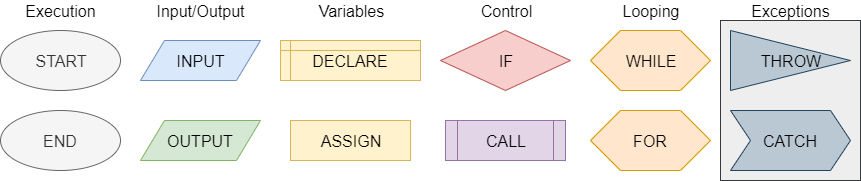
One method of representing computer programs is through the use of flowcharts. A flowchart consists of graphical blocks representing individual operations to be performed, connected with arrows which describe the flow of the program. The image above gives the basic building blocks of the flowcharts that will be used in this course. We will mostly follow the flowchart design used by the Flowgorithm program available online. The following pages in this chapter will introduce and discuss each block in detail.
We can also express our computer programs through the use of pseudocode. Pseudocode is an abstract language that resembles a high-level programming language, but it is written in such a way that it can be easily understood by any programmer who is familiar with any one of several common languages. The pseudocode may not be directly executable as written, but it should contain enough detail to be easily understood and adapted to an actual programming language by a skilled programmer.
There are many standards that exist for pseudocode, each with their own unique features and uses. In this course, we will mostly follow the standards from the International Baccalaureate Organization. In the following pages in this chapter, we’ll also introduce pseudocode for each of the flowchart blocks shown above.
Let’s discuss some of the basic concepts we need to understand about the Python programming language.
To begin, let’s look at a simple Hello World program written in Python:
def main():
    print("Hello World!")


# main guard
if __name__ == "__main__":
    main()
This program contains multiple important parts:
main(). Python does not require us to do this, since we can write our code directly in the file and it will execute. However, since we are going to be building larger programs in this course, it is a good idea to start using functions now.:, and then the code inside of that function comes directly after it. The code contained in the function must be indented a single level. By convention, Python files should use 4 spaces to indent the code. Thankfully, Codio does that for us automatically.main() function to run the program.Of course, this is a very brief overview for the Python programming language. To learn more, feel free to refer to the references listed below, as well as the textbook content for previous courses.
See if you can use the code above to write your own Hello World program a file named HelloWorld.py. We’ll learn how to compile and run that program on the next page.
Now that we’ve written our first Python program, we must run the program to see the fruits of our labors. There are many different ways to do this using the Codio platform. We’ll discuss each of them in detail here.
Codio includes a built-in Linux terminal, which allows us to perform actions directly on a command-line interface just like we would on an actual computer running Linux. We can access the Terminal in many ways:
Additionally, some pages may already open a terminal window for us in the left-hand pane, as this page so helpfully does. As we can see, we’re never very far away from a terminal.
No worries! We’ll give you everything you need to know to run your Python programs in this course.
If you’d like to learn a bit more about the Linux terminal and some of the basic commands, feel free to check out this great video on YouTube:
Let’s go to the terminal window and navigate to our program. When we first open the Terminal window, it should show us a prompt that looks somewhat like this one:
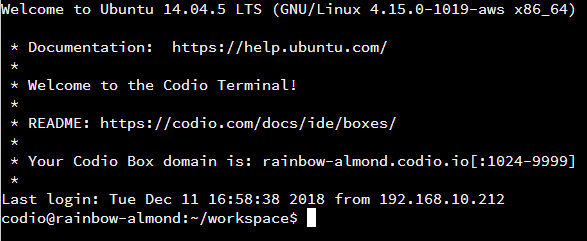
There is quite a bit of information there, but we’re interested in the last little bit of the last line, where it says ~/workspace. That is the current directory, or folder, our terminal is looking at, also known as our working directory. We can always find the full location of our working directory by typing the pwd command, short for “Print Working Directory,” in the terminal. Let’s try it now!
Enter this command in the terminal:
pwdand we should see output similar to this:
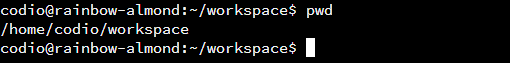
In that output, we’ll see that the full path to our working directory is /home/codio/workspace. This is the default location for all of our content in Codio, and it’s where everything shown in the file tree to the far left is stored. When working in Codio, we’ll always want to store our work in this directory.
Next, let’s use the ls command, short for “LiSt,” to see a list of all of the items in that directory:
ls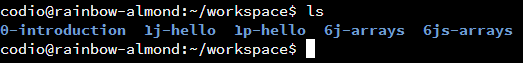
We should see a whole list of items appear in the terminal. Most of them are directories containing examples for the chapters this textbook, including the HelloWorld.py file that we edited in the last page. Thankfully, the directories are named in a very logical way, making it easy for us to find what we need. For example, to find the directory for Chapter 1 that contains examples for Python, look for the directory with the name starting with 1p. In this case, it would be 1p-hello.
Finally, we can use the cd command, short for “Change Directory,” to change the working directory. To change to the 1p-hello directory, type cd into the terminal window, followed by the name of that directory:
cd 1p-hello
We are now in the 1p-hello directory, as we can see by observing the ~/workspace/1p-hello on the current line in the terminal. Finally, we can do the ls command again to see the files in that directory:
ls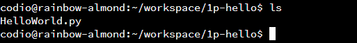
We should see our HelloWorld.py file! If it doesn’t appear, try using this command to get to the correct directory: cd /home/codio/workspace/1p-hello.
Once we’re at the point where we can see the HelloWorld.py file, we can move on to actually running the program.
To run it, we just need to type the following in the terminal:
python3 HelloWorld.py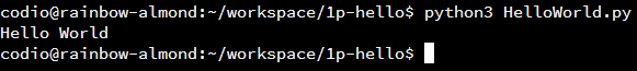
That’s all there is to it! We’ve now successfully run our first Python program. Of course, we can run the program as many times as we want by repeating the previous python3 command. If we make changes to the HelloWorld.py file that instruct the computer to do something different, we should see those changes the next time we run the file..
If the python3 command doesn’t give you any output, or gives you an error message, that most likely means that your code has an error in it. Go back to the previous page and double-check that the contents of HelloWorld.py exactly match what is shown at the bottom of the page. You can also read the error message output by python3 to determine what might be going wrong in your file.
Also, make sure you use the python3 command and not just python. The python3 command references the newer Python 3 interpreter, while the python command is used for the older Python 2 interpreter. In this book, we’ll be using Python 3, so you’ll need to always make sure you use python3 when you run your code.
We’ll cover information about simple debugging steps on the next page as well. If you get stuck, now is a great time to go to the instructors and ask for assistance. You aren’t in this alone!
See if you can change the HelloWorld.py file to print out a different message. Once you’ve changed it, use the python3 command to run the file again. Make sure you see the correct output!
Last, but not least, many of the Codio tutorials and projects in this program will include assessments that we must solve by writing code. Codio can then automatically run the program and check for specific things, such as the correct output, in order to give us a grade. For most of these questions, we’ll be able to make changes to our code as many times as we’d like to get the correct answer.
As we can see, there are many different ways to compile and run our code using Codio. Feel free to use any of these methods throughout this course.
Codio also includes an integrated debugger, which is very helpful when we want to determine if there is an error in our code. We can also use the debugger to see what values are stored in each variable at any point in our program.
To use the debugger, find the Debug Menu at the top of the Codio window. It is to the right of the Run Menu we’ve already been using. On that menu, we should see an option for Python - Debug File. Select that option to run our program in the Codio debugger.
As we build more complex programs in this course, we’ll be able to configure our own debugger configurations that allow us to test multiple files and operations.
The Codio debugger only works with input from a file, not from the terminal. So, to use the debugger, we’ll need to make sure the input we’d like to test is stored in a file, such as input.txt, before debugging. We can then give that file as an argument to our program in our debugger configuration, and write our program to read input from a file if one is provided as an argument.
Learning how to use a debugger is a hands-on process, and is probably best described in a video. You can find more information in the Codio documentation to get up to speed on working in the Codio debugger.
Codio Documentation - Debugger
We can always use the debugger to help us find problems in our code.
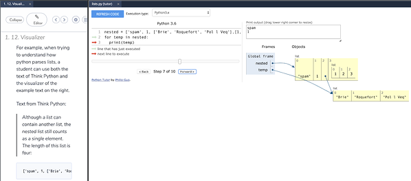
Codio now includes support for Python Tutor, allowing us to visualize what is happening in our code. We can see that output in the second tab that is open to the left.
Unfortunately, students are not able to open the visualizer directly, so it must be configured by an instructor in the Codio lesson. If you find a page in this textbook where you’d like to be able to visualize your code, please let us know!
A variable in a programming language is an abstraction that allows storing one value in each instant of time, but this value can change along with the program execution. A variable can be represented as a box holding a value. If the variable is a container, e.g., a list (or array or vector), a matrix, a tuple, or a set of values, each box in the container contains a single value.
A variable is characterized by:
results, number_of_nodes, number_of_edges. For writing variable names composed of two or more words in Python we can use underscores to separate the words.Depending on the programming language, we could also specify for a variable:
A programming language allows to perform two basic operations with a variable:
+, and subtraction -. They allow performing basic arithmetic operations with numbers.<, and greater than >. Usually, they allow to comparing two operands, each of which could be a variable. The result of the comparison is either the Boolean value true or the Boolean value false.and , or, and not. This operator allows us to relate logical conditions together to create more complex statements.+ to concatenate the strings “Hello” and the string “world” to produce the string “Hello world”. These operators allow us to manipulate strings.a = b.The table below lists the flowchart blocks used to represent variables, as well as the corresponding pseudocode:
| Operation | Flowchart | Pseudocode |
|---|---|---|
| Declare | 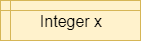
|
X = 0 |
| Assign | 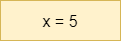
|
X = 5 |
| Declare & Assign | 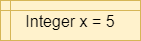
|
X = 5 |
Notice that variables must be assigned a value when declared in pseudocode. By default, most programming languages automatically assign the value $0$ to a new integer variable, so we’ll use that value in our pseudocode as well.
Likewise, variables in a flowchart are given a type, whereas variables in pseudocode are not. Instead, the data type of those variables can be inferred by the values stored in them.
Variables in Python are simply defined by giving them a value. The type of the variable in inferred from the data stored in it at any given time, and a variable’s type may change throughout the program as different values are assigned to it.
To define a variable, we can simply use an assignment statement to give it a value:
x = 5
y = 3.5We can also convert, or cast, data between different types. When we do this, the results may vary a bit due to how computers store and calculate numbers. So, it is always best to fully test any code that casts data between data types to make sure it works as expected.
To cast, we can simply use the new type as a function and place the value to be converted in parentheses:
x = 1.5
y = int(x)
This will convert the floating point value stored in x to an integer value stored in y.
The conditional statement, also known as the If-Then statement, is used to control the program’s flow by checking the value of a Boolean statement and determining if a block of code should be executed based on that value. This is the simplest conditional instruction. If the condition is true, the block enclosed within the statement is executed. If it is false, then the code in the block is skipped.
A more advanced conditional statement, the If-Then-Else or If-Else statement, includes two blocks. The first block will be executed if the Boolean statement is true. If the Boolean statement is false, then the second block of code will be executed instead.
Simple conditions are obtained by means of the relational operators, such as <, >, and ==, which allow you to compare two elements, such as two numbers, or a variable and a number, or two variables. Compound conditions are obtained by composing two or more simple conditions through the logical operators and, or, and not.
Recall that the Boolean logic operators and, or, and not can be used to construct more complex Boolean logic statements.
For example, consider the statement x <= 5. This could be broken down into two statements, combined by the or operation: x < 5 or x == 5. The table below, called a truth table, gives the result of the or operation based on the values of the two operands:
| Operand 1 | Operand 2 | Operand 1 or Operand 2 |
|---|---|---|
| False | False | False |
| False | True | True |
| True | False | True |
| True | True | True |
As shown above, the result of the or operation is True if at least one of the operands is True.
Likewise, to express the mathematical condition 3 < a < 5 we can use the logical operator and by dividing the mathematical condition into two logical conditions: a > 3 and a < 5. The table below gives the result of the and operation based on the values of the two operands:
| Operand 1 | Operand 2 | Operand 1 or Operand 2 |
|---|---|---|
| False | False | False |
| False | True | False |
| True | False | False |
| True | True | True |
As shown above, the result of the and operation is True if both of the operands are True.
Finally, the not logical operator is used to reverse, or invert, the value of a Boolean statement. For example, we can express the logical statement x < 3 as not (x >= 3), using the not operator to invert the value of the statement. The table below gives the result of the not operation based on the value of its operand:
| Operand | not Operand |
|---|---|
| False | True |
| True | False |
In propositional logic, the completeness theorem shows that all other logical operators can be obtained by appropriately combining the and, or and not operators. So, by just understanding these three operators, we can construct any other Boolean logic statement.
The table below lists the flowchart blocks used to represent conditional statements, as well as the corresponding pseudocode:
| Operation | Flowchart | Pseudocode |
|---|---|---|
| If-Then | 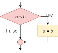
|
|
| If-Then-Else | 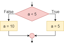
|
|
The mechanism for determining which block an If-Then-Else statement executes is the following:
To understand how a conditional statement works, let’s look at this example of a simple If-Then-Else statement. Consider the following flowchart:
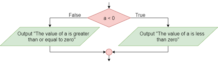
In this case, if a is less than zero, the output message will be “The value of a is less than zero”. Otherwise, if a is not less than zero (that is, if a is greater than or equal to zero), the output message will be “The value of a is greater than or equal to zero”.
We can also nest conditional statements together, making more complex programs.
Consider the following flowchart:
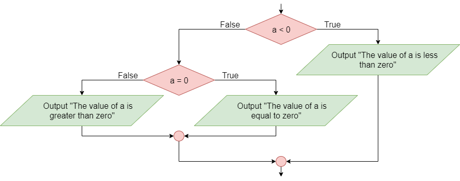
In this case, if a is less than zero the output message will be “The value of a is less than zero”. Otherwise (that is, if a is not less than zero so if a is greater than or equal to zero) the block checks whether a is equal to zero; if so, the output message will be “The value of a is equal to zero”. Otherwise (that is, if the first condition is false, i.e. a >= 0 and the second condition is false, i.e. is nonzero; the two conditions must be both true as if they were bound by a logical and, and they are the same as the condition a > 0) the output message will be “The value of a is greater than zero”.
To see how conditional statements look in Python, let’s recreate them from the flowcharts shown above.
if a < 5:
    a = 5
if a < 5:
    a = 5
else:
    a = 10
if a < 0:
    print("The value of a is less than zero")
elif a == 0:
    print("The value of a is equal to zero")
else:
    print("The value of a is greater than zero")
As we can see in the examples above, we must carefully indent each block of code to help set it apart from the other parts of the program. In addition, each line containing if, elif and else must end in a colon :.
Loops are another way we can control the flow of our program, this time by repeating steps based on a given criteria. A computer is able to repeat the same instructions many times. There are several ways to tell a computer to repeat a sequence of instructions:
while true. This construct is useful in software applications such as servers that will offer a service. The service is supposed to be available forever.Repeat 10 times or for i = 1 to 10. This loop can be used when you know the number of repetitions. There are also loops that allow you to repeat as many times as there are elements of a collection, such as for each item in listwhile loop, which repeats while the condition is true.In repeat while loops, the number of repetitions depends on the occurrence of a condition: the cycle repeats if the condition is true. Loops can also be nested, just like conditional statements.
The table below lists the flowchart blocks used to represent loop statements, as well as the corresponding pseudocode:
| Operation | Flowchart | Pseudocode |
|---|---|---|
| While Loop | 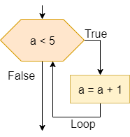
|
|
| For Loop | 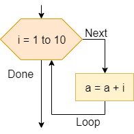
|
|
| For Loop with Step | 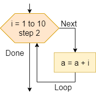
|
|
| For Each Loop | 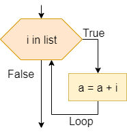
|
|
To see how loops look in Python, let’s recreate them from the flowcharts shown above.
while a < 5:
    a = a + 1
for i in range(1, 11):
    a = a + i
for i in range(1, 11, 2):
    a = a + i
for i in list:
    a = a + i
As we can see in the examples above, we must carefully indent each block of code to help set it apart from the other parts of the program. In addition, each line containing for and while must end in a colon :. Finally, notice that the range() function in Python does not include the second parameter in the output. So, to get the numbers $1$ through $10$, inclusive, we must use range(1, 11) in our code.
 ^[File:USPS Post office boxes 1.jpg. (2017, May 17). Wikimedia Commons, the free media repository. Retrieved 18:17, November 5, 2018 from https://commons.wikimedia.org/w/index.php?title=File:USPS_Post_office_boxes_1.jpg&oldid=244476438.]
Arrays allow us to store multiple values in the same variable, using an index to determine which value we wish to store or retrieve from the array. We can think of arrays like a set of post office boxes. Each one has the same physical address, the post office, but within the post office we can find an individual box based on its own box number.
Some programming languages, such as Java, use arrays that are statically sized when they are first created, and those arrays cannot be resized later. In addition, many languages that require variables to be declared with a type only allow a single variable type to be stored in an array.
Other languages, such as Python, use lists in place of arrays. List can be resized, and in untyped languages such as Python they can store different data types within the same list.
The table below lists the flowchart blocks used to represent arrays, as well as the corresponding pseudocode:
| Operation | Flowchart | Pseudocode |
|---|---|---|
| Declare Array | 
|
|
| Store Item | 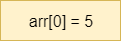
|
|
| Retrieve Item | 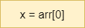
|
|
Let’s review the syntax for working with lists in Python.
To define a list in Python, we can simply place values inside of a set of square brackets [], separated by commas ,:
arr = [1, 2]
arr2 = [1.2, 3.4]
We can also create an empty list by simply omitting any items inside the square brackets
arr3 = []Once we’ve created a list in Python, we can add items to the end of the list using the append() method:
arr4 = []
arr4.append(1)
arr4.append(2)
arr4.append(3)Once the list is created, we can access individual items in the list by placing the index in square brackets [] after the list’s variable name:
x = arr[2]
arr[1] = 5Python lists can also be created with multiple dimensions, simply by appending lists as elements in a base list.
two_dim_arr = []
two_dim_arr.append([1, 2, 3])
two_dim_arr.append([4, 5, 6])
They can also be created through the use of lists as individual elements in a list when it is defined:
another_arr = [[1, 2, 3], [4, 5, 6]]To access elements in a multidimensional list, simply include additional sets of square brackets containing an index [] for each dimenison:
another_arr = [[1, 2, 3], [4, 5, 6]]
x = another_arr[1, 2]
another_arr[0, 1] = 5There are several operations that can be performed on lists in Python as well:
arr = [1, 2, 3, 4, 5]

# list length
length = len(arr)

# concatenation
arr2 = [6, 7]
arr3 = arr + arr2  # [1, 2, 3, 4, 5, 6, 7]

# slicing
b = arr[2:4] # [3, 4]Finally, we can use a special form of loop, called a For Each loop, to iterate through items in a list in Python:
arr = [1, 2, 3, 4 5]

for i in arr:
    print(i)
Once important thing to note is that lists accessed within a For Each loop are read only. So, we cannot change the values stored in the list using this loop, but we can access them. If we want to change them, we should use a standard For loop to iterate through the indices of the list:
arr = [1, 2, 3, 4, 5]

for i in range(0, len(arr)):
arr[i] = arr[i] + 5Variables in our programs can be used in a variety of different roles. The simplest role for any variable is to store a value that does not change throughout the entire program. Most variables, however, fit into one of several roles throughout the program.
To help us understand these roles, let’s review them in detail here. As we move forward in this course, we’ll see many different data structures that use variables in these ways, so it helps to know each of them early on!
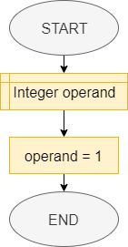
OPERAND = 1In this role, the variable is used to hold a value. This value can be changed during the program execution. In the example:
operand of type Integer is declared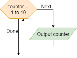
loop COUNTER from 1 to 10
    print COUNTER
end loop
In this role, variables are used to hold a sequence of values known beforehand. In the example, the variable counter holds values from 1 to 10 and these values are conveyed to the user.
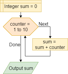
SUM = 0
loop COUNTER from 1 to 10
    SUM = SUM + COUNTER
end loop
print SUM
In this role, the variable is used to hold a value that aggregates, summarizes, and synthesize multiple values by means of an operation such as sum, product, mean, geometric mean, or median. In the example, we calculate the sum of the first ten numbers in the accumulator variable sum.
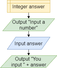
ANSWER = 0
print "Input a number"
input ANSWER
print "You input " + ANSWER
In this role, the variable answer contains the last value encountered so far in a data series, such as the last value that the program receives from the user.
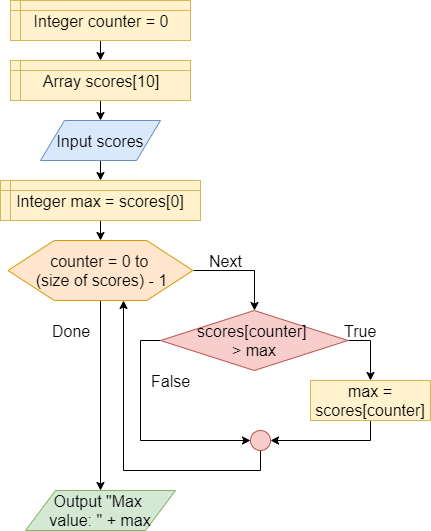
COUNTER = 0
SCORES = new array[10]
input SCORES
MAX = SCORES[0]
loop COUNTER from 0 to (size of SCORES) - 1
    if SCORES[COUNTER] > MAX
        MAX = SCORES[COUNTER]
    end if
end loop
print "Max value: " + MAX
In this role, the variable contains the value that is most appropriate for the purpose of the program, e.g. the minimum or the maximum. The instruction scores[counter] > max checks if the list item under observation is greater than the maximum. If the condition is true the value of the maximum variable is changed.
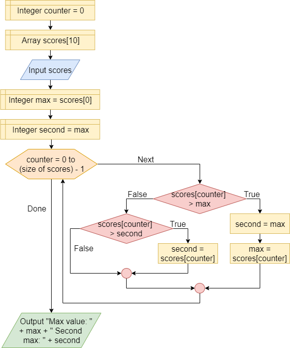
COUNTER = 0
SCORES = new array[10]
input SCORES
MAX = SCORES[0]
SECOND = MAX
loop COUNTER from 0 to (size of SCORES) - 1
    if SCORES[COUNTER] > MAX
        SECOND = MAX
        MAX = SCORES[COUNTER]
    else if SCORES[COUNTER] > SECOND
        SECOND = SCORES[COUNTER]
    end if
end loop
print "Max value: " + MAX + " Second max: " + SECOND
A variable, such as second, to which you assign the value of another variable that will be changed immediately after. In the example, the second variable contains the second largest value in a list.
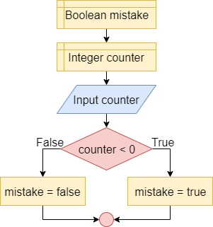
MISTAKE = false
COUNTER = 0
input COUNTER
if COUNTER < 0
    MISTAKE = true
else
    MISTAKE = false
end if
A flag variable is used to report the occurrence or not of a particular condition, e.g. the occurrence of an error, the first execution, etc..
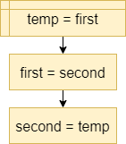
TEMP = FIRST
FIRST = SECOND
SECOND = TEMP
A variable used to hold a temporary value. For example, to exchange two variables, you must have a temporary variable temp to store a value before it is replaced.
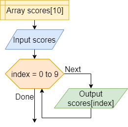
SCORES = new array[10]
input SCORES
loop INDEX from 0 to 9
    print SCORES[INDEX]
end loop
A variable used to indicate the position of the current item in a set of elements, such as the current item in an array of elements. The index variable here is a great example.
Strings are another very important data type in programming. A string is simply a set of characters that represent text in our programs. We can then write programs that use and manipulate strings in a variety of ways, allowing us to easily work with textual data.
The table below lists the flowchart blocks used to represent strings, as well as the corresponding pseudocode:
| Operation | Flowchart | Pseudocode |
|---|---|---|
| Create String | 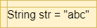
|
|
| Access Character | 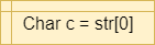
|
|
| String Length | 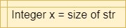
|
|
Let’s review the syntax for working with strings in Python.
Strings in Python are declared just like any other variable:
s = "abc123"Notice that strings are enclosed in double quotations marks ". Since Python does not have a data type for a single character, we can do the same for single character strings as well:
c = "a"There are several special characters we can include in our strings. Here are a few of the more common ones:
\' - Single Quotation Mark (usually not required)\" - Double Quotation Mark\n - New Line\t - TabMost of the time, we will need to be able to parse strings in order to read input from the user. This is easily done using Python. Let’s refer to the skeleton code given in an exercise:
# Load required modules
import sys


def main(argv):

    # create a file reader for terminal input
    reader = sys.stdin

    # read a single integer from the terminal
    x = int(reader.readline())

    # -=-=-=-=- MORE CODE GOES HERE -=-=-=-=-


# main guard
if __name__ == "__main__":
    main(sys.argv)
This code will initialize a variable called reader to read input from the terminal, or sys.stdin in Python.
Once we have a reader initialized, we can read a line of data from the input as follows:
line = reader.readline()If we know that line will contain a single item of a different data type, such as an integer, we can also convert that input using the appropriate method:
x = int(reader.readline())Finally, if we have read an entire string of input consisting of multiple parts, we can use the split method to split the string in to tokens that are separated by a special delimiter. When we do this, we’ll have to use special methods to convert the strings to other primitive data types. Here’s an example:
line = "This 1 is 2.0 true"
parts = line.split(" ")
first = parts[0]
second = int(parts[1])
third = parts[2]
fourth = float(parts[3])
fifth = bool(parts[4])
In this example, we are able to split the first string variable into $5$ parts, each one separated by a space in the original string. Then, we can use methods such as int() to convert each individual string token into the desired data type.
When reading an unknown number of lines of input, we can use a loop in Python such as the following example:
for line in reader:
    line = line.strip()
    if not line or len(line) == 0:
        break

    # parse the input
This will read input until either a blank line is received (usually via the terminal), or there is no more input available to read (from a file).
There are also several operations we can perform on strings in Python:
s1 = "This"
s2 = "That"

# string length
x = len(s1)

# string comparison
# can use standard comparison operators
b1 = s1 == s2
b2 = s1 < s2

# concatenation
s3 = s1 + " " + s2
Additional methods can be found on the Python Built-In Types: str and Python Common String Operations pages
Strings can also be used to create formatted output in Python through the use of f-strings. Here’s a short example:
sum = 123
avg = 1.23
name = "Student"

print(f"{name}: Your score is {sum} with an average of {avg}.")
When we run this program, the output will be:
Student: Your score is 123 with an average of 1.23.Each item in the formatted output can also be given additional attributes such as width and precision. More details can be found on the Python Format String Syntax page.
An exception is an error that a program encounters when it is running. While some errors cannot be dealt with directly by the program, many of these exceptions can be caught and handled directly in our programs.
There isn’t really a standard way to display exceptions in flowcharts and pseudocode, but we can easily create a system that works well for our needs. Below are the flowchart blocks and pseudocode examples we’ll use in this course to represent exceptions and exception handling:
| Operation | Flowchart | Pseudocode |
|---|---|---|
| Throw Exception | 
|
|
| Catch Exception | 
|
|
| Try-Catch Example | 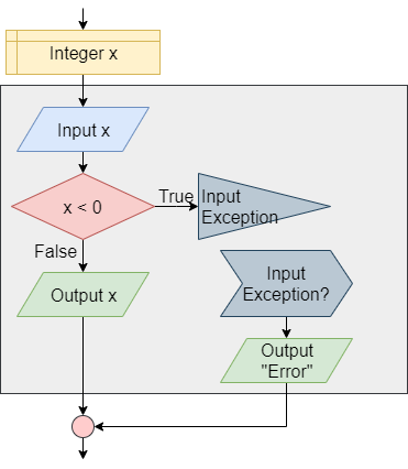
|
|
Let’s review the syntax for working with exceptions in Python.
In Python, we can use a Try-Except statement to detect and handle exceptions in our code:
# Load required modules
import sys

try:
    reader = open(sys.argv[1])
    x = int(reader.readline())
    print(x)

except Exception as e:
    print("Error!")
In this example, the program will try to open a file using the first command-line argument as a file name. There are several exceptions that could occur in this code, such as a ValueError, a IndexError, a FileNotFoundError, and more. They can also be handled individually:
# Load required modules
import sys

try:
    reader = open(sys.argv[1])
    x = int(reader.readline())
    print(x)

except IndexError as e:
    print("Error: Invalid Array Index!")
except FileNotFoundError as e:
    print("Error: File Not Found!")
except ValueError as e:
    print("Error: Input Does Not Match Expected Format!")
except OSError as e:
print("Error: OS Exception!")If desired, we can also raise our own exceptions in Python:
if y == 0:
    raise ValueError("Cannot divide by zero")
else:
    z = x / y
    print(z)
This will cause an exception to be thrown if the value of y is equal to $0.0$.
We can also add Else and Finally blocks at the end of each Try-Except block. A Finally block will be executed whenever the control exits the Try-Except block, even through the use of a return statement to return from a method. The Else block will be executed if the entire Try-Except block completes without any exceptions being raised:
# Load required modules
import sys

try:
    reader = open(sys.argv[1])
    x = int(reader.readline())
    print(x)

except Exception as e:
    print("Error!")
else:
    print("No Errors!")
finally:
print("Finally Block")When working with resources such as files in Python, we can also use a With block to ensure that those resources are properly closed when we are done with them. In addition, a With block will automatically catch and suppress any exceptions that result from trying to close the resource after an exception has occurred, preventing us from being bombarded by unavoidable exceptions. Here’s an example:
import sys

try:
    with open(sys.argv[1]) as reader:
        x = int(reader.readline())
        print(x)

except IndexError as e:
    print("Error: Invalid Array Index!")
except ValueError as e:
    print("ValueError: {}".format(e))
except FileNotFoundError as e:
    print("FileNotFoundError: {}".format(e))
In this example, we are opening a file using the open() method inside of the With statement. That file will automatically be closed once the program leaves the With statement.
One of the major features of a modern computer is the ability to store and retrieve data from the computer’s file system. So, we need to be able to access the file system in our code in order to build useful programs. Thankfully, most modern programming languages include a way to do this.
Most operations working with files in code take the form of method calls. So, we will primarily use the call block to represent operations on files:
| Operation | Flowchart | Pseudocode |
|---|---|---|
| Open File | 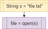
|
|
| Read from File | 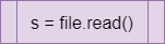
|
|
| Write to File | 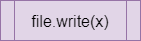
|
|
Let’s review the syntax for working with files in Python.
To open a file in Python, we can simply use the open() method. Here is an example:
import sys

try:
    reader = open(sys.argv[1])
except FileNotFoundError as e:
    print("FileNotFoundError: {}".format(e))
    sys.exit()
except IndexError as e:
    print("IndexError: {}".format(e))
    reader = sys.stdin

with reader:
    # -=-=-=-=- MORE CODE GOES HERE -=-=-=-=-
In this example, the program will try to open a file provided as the first command-line argument. If no argument is provided, it will automatically read from standard input instead. However, if an argument is provided, it will try to open it as a file. In addition, we can use a With statement to make sure the file is properly closed once it is open.
Once we have opened the file, we can read the file just like we would any other input:
for line in reader:
    line = line.strip()
    if not line or len(line) == 0:
        break
# use line variableTo write to a file, we must open it a different way. In Python, we must provide an optional "w" argument to the open() method call to make the file writable:
import sys

try:
    with open(sys.argv[1], "w") as writer:
        writer.write("Hello World")
        writer.write("\n")

except IndexError as e:
    # no arguments provided
    print("IndexError: {}".format(e))
    sys.exit()
except IOError as e:
    # unable to write to the file
    print("IOError: {}".format(e))
    sys.exit()
except Exception as e:
    # unknown exception
    print("Exception: {}".format(e))
    sys.exit()
This example shows to how to open a file for writing using the open() method inside of a With statement. It also lists several of the common exceptions and their cause.
It is important both to easily grasp the design choice and the code structure of a project even long after it has been completed. The documentation process starts by commenting the code. Code comments are usually intended for software developers and aim at clarifying the code by giving details of how it works. They are usually performed using inline or multiple lines comments using the language syntax.
As we’ve seen before, we can add single-line comments to our Python programs using a hash symbol # before a line in our source file:
# this is a comment
x = 5

# this is also a comment
b = TrueFinally, Python also includes a secondary type of comment that spans multiple lines, specifically for creating documentation. A docstring is usually the first line of text inside of a class or method definition, and is surrounded by three double quotes """ with one set of three on each end.
These comments are specifically designed to provide information about classes and methods in our code. Here’s a quick example using a simple class:
class IntTuple:
  """ Represents a tuple containing two integer values

  This class is an adaptation of a class developed for Java
  that mimics the built-in tuples in Python

  Attributes
  ----------
  first : int
      the first element in the tuple
  second : int
      the second element in the tuple
  """

  def __init__(self, one, two):
    """ Initializes a new IntTuple object

    Parameters
    ----------
    one : int
        the first element in the new tuple
    two : int
        the second element in the new tuple
    """
    self.first = one
    self.second = two
Unfortunately, Python does not enforce a particular style for these docstrings, so there are many different formats used in practice. To learn more, we can consult the following references.
To make your code easier to read, many textbooks and companies use a style guide that defines some of the formating rules that you should follow in your source code. In Python, these rules are very important, as the structure of your code is defined by the layout. We’ll learn more about that in a later module.
For this book, most of the examples will be presented using the guidelines in the Style Guide for Python. However, by default Codio used to use 2 spaces for an indentation level instead of 4, so that is the format that will be used in some examples in this book.
Google also provides a comprehensive style guide that is recommended reading if you’d like to learn more about how to format your source code.
That’s a quick overview of the basics we’ll need to know before starting the new content in this course. The next module will provide a quick review of object-oriented programming concepts as well as the model-view-controller or MVC architecture, both of which will be used heavily in this course.
Review Object-Oriented Programming in Python
Object-oriented programming uses the idea of objects and classes to provide many improvements over other programming paradigms. The key concept of object-oriented programming - encapsulation - allows our data and the operations that manipulate that data to be bundled together within a single object.
File:CPT-OOP-inheritance.svg. (2014, June 26). Wikimedia Commons, the free media repository. Retrieved 01:22, January 14, 2020 from https://commons.wikimedia.org/w/index.php?title=File:CPT-OOP-inheritance.svg&oldid=127549650. ↩︎
Functions are small pieces of reusable code that allow you to divide complex programs into smaller subprograms. Ideally, functions perform a single task and return a single value. (It should be noted that some programming languages allow for procedures, which are similar to functions but return no values. Except for the return value, it is safe to group them with functions in our discussion below.)
Functions can be thought of as black boxes. When we talk about black boxes we mean that users cannot look inside the box to see how it actually works. A good example of a black box is a soda machine. We all use them and know how to operate them, but very few of actually know how they work inside. Nor do we really want to know. We are happy to simply use them machine and have it give a nice cold soda when we are thirst!
To be able to reuse functions easily, it is important to define what a function does and how it should be called.
Before we can call a function, we must know the function’s signature. A function’s signature includes the following.
While a signature will allow us to actually call the function in code. Of course to use functions effectively, we must also know exactly what the function is supposed to do. We will talk more about how we do this in the next module on programming by contract. For now we can assume that we just have a good description of what the function does.
While we do not need to know exactly how a function actually performs its task, the algorithm used to implement the function is vitally important as well. We will spend a significant amount of time in this course designing such algorithms.
The lifecycle of a function is as follows.
When the function is called, the arguments, or actual parameters, are copied to the function’s formal parameters and program execution jumps from the “call” statement to the function. When the function finishes execution, execution resumes at the statement following the “call” statement.
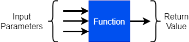
In general, parameters are passed to functions by value, which means that the value of the calling program’s actual parameter is copied into the function’s formal parameter. This allows the function to modify the value of the formal parameter without affecting the actual parameter in the calling program.
However, when passing complex data structures such as objects, the parameters are passed by reference instead of by value. In this case, a pointer to the parameter is passed instead of a copy of the parameter value. By passing a pointer to the parameter, this allows the function to actually make changes to the calling program’s actual parameter.
As you might guess from its name, object-oriented programming languages are made to create and manipulate entities called objects. But what exactly are these objects? Objects were created to help decompose large complex programs with a lot of complex data into manageable parts.
An object is a programming entity that contains related data and behavior.
A good example of an object is dog. But not just any dog, or all dogs, but a specific dog. Each dog has specific characteristics that are captured as data such as their name, their height, their weight, their breed, their age, etc. We call these characteristics attributes and all dogs have the same type of attributes, although the values of those attributes may be unique. And generally, all dogs exhibit the same behaviors, or methods. Almost all dogs can walk, run, bark, eat, etc.
So, how do we define the basic attributes and behaviors of a dog? We probably start with some kind of idea of what a dog is. How do we describe dogs in general. In object orientation we do that through classes.
A class is a blueprint for an object.
What do we use blueprints for? Well, when we are building a physical structure such as a home or office building, an architect first creates a blueprint that tells the builder what to build and how everything should fit together. That is essentially what a class does. A class describes the types of attributes and methods that an object of that class will have.
Then to create objects, we say we create an instance of a class by calling the class’s constructor method, which creates an object instance in memory and makes sure it’s attributes are properly created. Once the object has been created, the methods defined by the class can be used to manipulate the attributes and internal data of the object.
Two of the most powerful concepts in object orientation are encapsulation and information hiding.
Encapsulation enables information hiding, and information hiding allows us to simplify the interface used to interact with an object. Instead of needing to know everything about a particular class of objects in order to use or interact with those objects. This will make our programs less complex and easier to implement and test. It also makes it easier for you to change the internal implementations of methods without affecting the rest of your program. As long as the method behaves in the same way (i.e., produces the same outputs given a given set of inputs), the rest of your program will not be affected. Thus, we see two key parts of any class:
Encapsulation and information hiding are actually all around us. Take for example, a soda vending machine. There are many internal parts to the machine. However, as a user, we care little about how the machine works or what it does inside. We need to simply know how to insert money or swipe our card and press a couple of buttons to get the soda we desire. If a repair is needed and an internal motor is replaced, we don’t care whether they replaced the motor with the exact same type of motor or the new model. As long as we can still get our soda by manipulating the same payment mechanisms and buttons, we are happy. You and I care only about the interface to the machine, not the implementation hiding inside.
To implement information hiding in our classes, we use visibility. In general, attributes and methods can either be public or private. If we want and attribute or method to be part of the class interface, we define them as public. If we want to hide a attribute or method from external objects, we defined them as private. An external object may access public attributes and call public methods, which is similar to using the payment mechanism or the buttons on a soda machine. However, the internals of how the object works is hidden by private attributes and methods, which are equivalent to the internal workings of the soda machine.
To implement information hiding, we recommend that you declare all attributes of a class as private. Any attribute whose value should be able to be read or changed by an external object should create special “getter” and “setter” methods that access those private variables. This way, you can make changes to the implementation of the attributes without changing how it is accessed in the external object.
Polymorphsim is a concept that describes the fact that similar objects tend to behave in similar ways, even if they are not exactly alike. For example, if we might have a set of shapes such as a square, a circle, and a rhombus. While each shape shares certain attributes like having an area and a perimeter. However, each shape is also unique and may have differing number of sides and angles between those sides, or in the case of a circle, a diameter. We describe this relationship by saying a circle (or rectangle, or rhombus) “is a” shape as shown in the figure below.
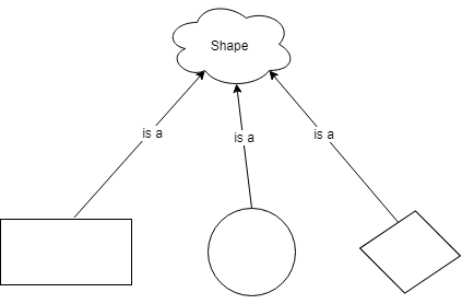
Inheritance is a mechanism that captures polymorphism by allowing classes to inherit the methods and attributes from another class. The basic purpose of inheritance to to reuse code in a principled and organized manner. We generally call the inheriting class the subclass or child class, while the class it inherits from is called the superclass or parent class.
Basically, when class ‘A’ inherits from class ‘B’, all the methods and attributes of class ‘A’ are automatically copied to class ‘B’. Class ‘B’ can then add additional methods or attributes to extend class ‘A’, or overwrite the implementations of methods in class ‘A’ to specialize it.
When programming, we use inheritance to implement polymorphism. In our shape example, we would have a generic (or abstract) Shape class, which is inherited by a set of more specific shape classes (or specializations) as shown below.
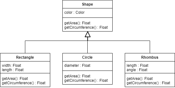
In this example, the Shape class defines the ‘color’ attribute and the ‘getArea’ and ‘getCircumference’ methods, which are inherited by the Rectangle, Circle, and Rhombus classes. Each of the subclasses define additional attributes that are unique to the definition of each shape type.
Notice that although the Shape class defines the signatures for the ‘getArea’ and ‘getCircumference’ methods, it cannot define the implementation of the methods, since this is unique to each subclass shape. Thus, each subclass shape will specialize the Shape class by implementing their own ‘getArea’ and ‘getCircumference’ methods.
So far, we have discussed Single inheritance, which occurs when a class has only one superclass. However, theoretically, a class may inherit from more than one superclass, which is termed multiple inheritance. While a powerful mechanism, multiple inheritance also introduces complexity into understanding and implementing programs. And, there is always the possibility that attributes and methods from the various superclasses contradict each other in the subclass.
For object a to be able to call a method in object b, object a must have a reference (a pointer, or the address of) object b. In many cases, objects a and b will be in a long-term relationship so that one or both objects will need to store the reference to the other in an attribute. When an object holds a reference to another object in an attribute, we call this a link. Examples of such relationships include a driver owning a car, a person living at an address, or a worker being employed by a company.
As we discussed earlier, objects are instances of classes. To represent this in a UML class diagram, we use the notion of an association, which is shown as a line connecting to two classes. More precisely, a link is an instance of an association. The figure belows shows three examples of an association between class A and class B.
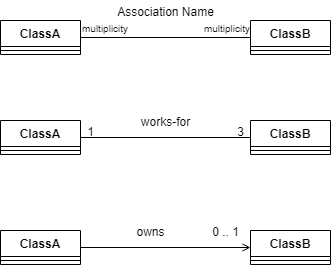
The top example shows the basic layout of an association in UML. The line between the two classes denotes the association itself. The diagram specifies that ClassA is associated with ClassB and vice versa. We can name the association as well as place multiplicities on the relationships. The multiplicities show exactly how many links an object of one class must have to objects of the associated class. The general form a multiplicity is n .. m, which means that an object must store at least n, but no more than m references to other objects of the associated class; if only one number is given such as n, then the object must store exactly n references to objects in the associated class.
There are two basic types of associations.
The middle example shows a two-way association between ClassA and ClassB. Furthermore, each object of ClassA must have a link to exactly three objects of ClassB, while each ClassB object must have a link with exactly one ClassA object. (Note that the multiplicity that constrains ClassA is located next to ClassB, while the multiplicity that constrains ClassB is located next to ClassA.)
The bottom example shows a one-way association between ClassA and ClassB. In this case, ClassA must have links to either zero or one objects of ClassB. Since it is a one-way association, ClassB will have no links to objects of ClassA.
In Python, we can break our programs up into individual functions, which are individual routines that we can call in our code. Let’s review how to create functions in Python.
The table below lists the flowchart blocks used to represent functions, as well as the corresponding pseudocode:
| Operation | Flowchart | Pseudocode |
|---|---|---|
| Declare Function | 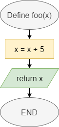
|
|
| Call Function | 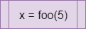
|
|
In general, a function definition in Python needs a few elements. Let’s start at the simplest case:
def foo():
  print("Foo")
  return
Let’s break this example function definition down to see how it works:
def at the beginning of this function definition. That keyword tells Python that we’d like to define a new function. We’ll need to include it at the beginning of each function definition.foo. We can name a function using any valid identifier in Python. In general, function names in Python always start with a lowercase letter, and use underscores between the words in the function name if it contains multiple words.() that list the parameters for this function. Since there is nothing included in this example, the function foo does not require any parameters.: indicating that the indented block of code below this definition is contained within the function. In this case, the function will simply print Foo to the terminal.return keyword. Since we aren’t returning a value, we aren’t required to include a return keyword in the function. However, it is helpful to know that we may use that keyword to exit the function at any time.Once that function is created, we can call it using the following code:
foo()In a more complex case, we can declare a function that accepts parameters and returns a value, as in this example:
def count_letters(input, letter):
  output = 0
  for i in range(0, len(input)):
    if input[i] == letter:
      output += 1
  return output
In this example, the function accepts two parameters: input, which could be a string, and letter, which could be a single character. However, since Python does not enforce a type on these parameters, they could actually be any value. We could add additional code to this function that checks the type of each parameter and raises a TypeError if they are not the expected type.
We can use the parameters just like any other variable in our code. To return a value, we use the return keyword, followed by the value or variable containing the value we’d like to return.
To call a function that requires parameters, we can include values as arguments in the parentheses of the function call:
sum += count_letters("The quick brown fox jumped over the lazy dog", "e")Python allows us to specify default values for parameters in a function definition. In that way, if those parameters are not provided, the default value will be used instead. So, it may appear that there are multiple functions with the same name that accept a different number of parameters. This is called function overloading.
For example, we could create a function named max() that could take either two or three parameters:
def main():
  max(2, 3)
  max(3, 4, 5)

def max(x, y, z=None):
  if z is not None:
    if x >= y:
      if x >= z:
        print(x)
      else:
        print(z)
    else:
      if y >= z:
        print(y)
      else:
        print(z)
  else:
    if x >= y:
      print(x)
    else:
      print(y)

# main guard
if __name__ == "__main__":
  main()
In this example, we are calling max() with both 2 and 3 arguments from main(). When we only provide 2 arguments, the third parameter will be given the default value None, which is a special value in Python showing that the variable is empty. Then, we can use if z is not None as part of an If-Then statement to see if we need to take that variable into account in our code.
This example also introduces a new keyword, is. The is keyword in Python is used to determine if two variables are exactly the same object, not just the same value. In this case, we want to check that z is exactly the same object as None, not just that it has the same value. In Python, it is common to use the is keyword when checking to see if an optional parameter is given the value None. We’ll see this keyword again in a later chapter as we start dealing with objects.
Python also allows us to specify function arguments using keywords that match the name of the parameter in the function. In that way, we can specify the arguments we need, and the function can use default values for any unspecified parameters. Here’s a quick example:
def main():
  args(1)             # 6
  args(1, 5)          # 9
  args(1, c=5)        # 8
  args(b=7, a=2)      # 12
  args(c=5, a=2, b=3) # 10

def args(a, b=2, c=3):
  print(str(a + b + c))

# main guard
if __name__ == "__main__":
  main()
In this example, the args() method has one required parameter, a. It can either be provided as the first argument, known as a positional argument, or as a keyword argument like a=2. The other parameters, b and c, can either be provided as positional arguments or keyword arguments, but they are not required since they have default values.
Also, we can see that when we use keyword arguments we do not have to provide the arguments in the order they are defined in the function’s definition. However, any arguments provided without keywords must be placed at the beginning of the function call, and will be matched positionally with the first parameters defined in the function.
Finally, Python allows us to define a single parameter that is a variable length parameter. In essence, it will allow us to accept anywhere from 0 to many arguments for that single parameter, which will then be stored in a list. Let’s look at an example:
def main():
  max(2, 3)
  max(3, 4, 5)
  max(5, 6, 7, 8)
  max(10, 11, 12, 13, 14, 15, 16)

def max(*values):
  if len(values) > 0:
    max = values[0]
    for value in values:
      if value > max:
        max = value
    print(max)

# main guard
if __name__ == "__main__":
  main()
Here, we have defined a function named max() that accepts a single variable length parameter. To show a parameter is variable length we use an asterisk * before variable name. We must respect two rules when creating a variable length parameter:
So, when we run this program, we see that we can call the max() function with any number of arguments, and it will be able to determine the maximum of those values. Inside of the function itself, values can be treated just like a list.
In programming, a class describes an individual entity or part of the program. In many cases, the class can be used to describe an actual thing, such as a person, a vehicle, or a game board, or a more abstract thing such as a set of rules for a game, or even an artificial intelligence engine for making business decisions.
In object-oriented programming, a class is the basic building block of a larger program. Typically each part of the program is contained within a class, representing either the main logic of the program or the individual entities or things that the program will use.
We can represent the contents of a class in a UML Class Diagram. Below is an example of a class called Person:
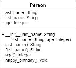
Throughout the next few pages, we will realize the design of this class in code.
To create a class in Python, we can simply use the class keyword at the beginning of our file:
class Person:
    pass
As we’ve already learned, each class declaration in Python includes these parts:
class - this keyword says that we are declaring a new class.Person - this is an identifier that gives us the name of the class we are declaring.Following the declaration, we see a colon : marking the start of a new block, inside of which will be all of the fields and methods stored in this class. We’ll need to indent all items inside of this class, just like we do with other blocks in Python.
In order for Python to allow this code to run, we cannot have an empty block inside of a class declaration. So, we can add the keyword pass to the block inside of the class so that it is not empty.
By convention, we would typically store this class in a file called Person.py.
Of course, our classes are not very useful at this point because they don’t include any attributes or methods. Including attributes in a class is one of the simplest uses of classes, so let’s start there.
To add an attribute to a class, we can simply declare a variable inside of our class declaration:
class Person:
    last_name = "Person"
    first_name = "Test"
    age = 25
That’s really all there is to it! These are static attributes or class attributes that are shared among all instances of the class. On the next page, we’ll see how we can create instance attributes within the class’s constructor.
Finally, we can make these attributes private by adding two underscores to the variable’s name. We denote this on our UML diagram by placing a minus - before the attribute or method’s name. Otherwise, a + indicates that it should be public. In the diagram above, each attribute is private, so we’ll do that in our code:
class Person:
    __last_name = "Person"
    __first_name = "Test"
    __age = 25
Unfortunately, Python does have a way to get around these restrictions as well. Instead of referencing __last_name, we can instead reference _Person__last_name to find that value, as in this example:
ellie = Person("Jonson", "Ellie", 29)
ellie._Person__last_name = "Jameson"
print(ellie.last_name) # Jameson
Behind the scenes, Python adds an underscore _ followed by the name of the class to the beginning of any class attribute or method that is prefixed with two underscores __. So, knowing that, we can still access those attributes and methods if we want to. Thankfully, it’d be hard to do this accidentally, so it provides some small level of security for our data.
We can also add methods to our classes. These methods are used either to modify the attributes of the class or to perform actions based on the attributes stored in the class. Finally, we can even use those methods to perform actions on data provided as arguments. In essence, the sky is the limit with methods in classes, so we’ll be able to do just about anything we need to do in these methods. Let’s see how we can add methods to our classes.
A constructor is a special method that is called whenever a new instance of a class is created. It is used to set the initial values of attributes in the class. We can even accept parameters as part of a constructor, and then use those parameters to populate attributes in the class.
Let’s go back to the Person class example we’ve been working on and add a simple constructor to that class:
class Person:
    __last_name = "Person"
    __first_name = "Test"
    __age = 25

    def __init__(self, last_name, first_name, age):
        self.__last_name = last_name
        self.__first_name = first_name
        self.__age = age
Since the constructor is an instance method, we need to add a parameter to the function at the very beginning of our list of parameters, typically named self. This parameter is automatically added by Python whenever we call an instance method, and it is a reference to the current instance on which the method is being called. We’ll learn more about this later.
Inside that constructor, notice that we use each parameter to set the corresponding attribute, using the self keyword once again to refer to the current object.
Also, since we are now defining the attributes as instance attributes in the constructor, we can remove them from the class definition itself:
class Person:

    def __init__(self, last_name, first_name, age):
        self.__last_name = last_name
        self.__first_name = first_name
self.__age = ageWe’ve already discussed variable scope earlier in this course. Recall that two different functions may use the same local variable names without affecting each other because they are in different scopes.
The same applies to classes. A class may have an attribute named age, but a method inside of the class may also use a local variable named age. Therefore, we must be careful to make sure that we access the correct variable, using the self reference if we intend to access the attribute’s value in the current instance. Here’s a short example:
class Test:
  age = 15

  def foo(self):
    age = 12
    print(age)      # 12
    print(self.age) # 15

  def bar(self):
    print(self.age) # 15
    print(age)      # NameError
As we can see, in the method foo() we must be careful to use self.age to refer to the attribute, since there is another variable named age declared in that method. However, in the method bar() we see that age itself causes a NameError since there is no other variable named age defined in that scope. We have to use self.age to reference the attribute.
So, we should always get in the habit of using self to refer to any attributes, just to avoid any unintended problems later on.
In Python, we can use a special decorator @property to define special methods, called getters and setters, that can be used to access and update the value of private attributes.
In Python, a getter method is a method that can be used to access the value of a private attribute. To mark a getter method, we use the @property decorator, as in the following example:
class Person:

    def __init__(self, last_name, first_name, age):
        self.__last_name = last_name
        self.__first_name = first_name
        self.__age = age

    @property
    def last_name(self):
        return self.__last_name

    @property
    def first_name(self):
        return self.__first_name

    @property
    def age(self):
return self.__ageSimilarly, we can create another method that can be used to update the value of the age attribute:
class Person:

    def __init__(self, last_name, first_name, age):
        self.__last_name = last_name
        self.__first_name = first_name
        self.__age = age

    @property
    def last_name(self):
        return self.__last_name

    @property
    def first_name(self):
        return self.__first_name

    @property
    def age(self):
        return self.__age
    @age.setter
    def age(self, value):
        self.__age = value
However, this method is not required in the UML diagram, so we can omit it.
To add a method to our class, we can simply add a function declaration inside of our class.
class Person:

    def __init__(self, last_name, first_name, age):
        self.__last_name = last_name
        self.__first_name = first_name
        self.__age = age

    @property
    def last_name(self):
        return self.__last_name

    @property
    def first_name(self):
        return self.__first_name

    @property
    def age(self):
        return self.__age

    def happy_birthday(self):
        self.__age = self.age + 1
Notice that once again we must remember to add the self parameter as the first parameter. This method will update the private age attribute by one year.
Now that we have fully constructed our class, we can use it elsewhere in our code through the process of instantiation. In Python, we can simply call the name of the class as a method to create a new instance, which calls the constructor, and then we can use dot-notation to access any attributes or methods inside of that object.
from Person import *

john = Person("Smith", "John", 25)
print(john.last_name)
john.happy_birthday()
Notice that we don’t have to provide a value for the self parameter when we use any methods. This parameter is added automatically by Python based on the value of the object we are calling the methods from.
We can also build classes that inherit attributes and methods from another class. This allows us to build more complex structures in our code, better representing the relationships between real world objects.
As we learned earlier in this chapter, we can represent an inheritance relationship with an open arrow in our UML diagrams, as shown below:
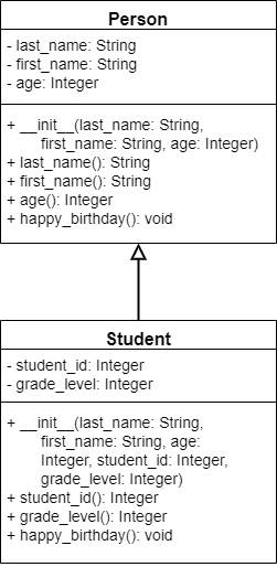
In this diagram, the Student class inherits from, or is a subclass of, the Person class.
To show inheritance in Python, we place the parent class inside of parentheses directly after the name of the subclass when it is defined:
from Person import *

class Student(Person):
    pass
From there, we can quickly implement the code for each property and getter method in the new class:
from Person import *

class Student(Person):

    @property
    def student_id(self):
        return self.__student_id

    @property
    def grade_level(self):
return self.__grade_levelSince the subclass Student also includes a definition for the method happy_birthday(), we say that that method has been overridden in the subclass. We can do this by simply creating the new method in the Student class, making sure it accepts the same number of parameters as the original:
from Person import *

class Student(Person):

    @property
    def student_id(self):
        return self.__student_id

    @property
    def grade_level(self):
        return self.__grade_level

    def happy_birthday(self):
        super().happy_birthday()
        self.__grade_level += 1
Here, we are using the function super() to refer to our parent class. In that way, we can still call the happy_birthday() method as defined in Person, but extend it by adding our own code as well.
In addition, we can use the super() method to call our parent class’s constructor.
from Person import *

class Student(Person):

    @property
    def student_id(self):
        return self.__student_id

    @property
    def grade_level(self):
        return self.__grade_level

    def __init__(self, last_name, first_name, age, student_id, grade_level):
        super().__init__(last_name, first_name, age)
        self.__student_id = student_id
        self.__grade_level = grade_level

    def happy_birthday(self):
        super().happy_birthday()
self.__grade_level += 1In addition to private and public attributes and methods, UML also includes the concept of protected methods. This modifier is used to indicate that the attribute or method should not be accessed outside of the class, but will allow any subclasses to access them. Python does not enforce this restriction; it is simply convention. In a UML diagram, the protected keyword is denoted by a hash symbol # in front of the attribute or method. In Python, we then prefix those attributes or methods with a single underscore _.
Inheritance allows us to make use of polymorphism in our code. Loosely polymorphism allows us to treat an instance of a class within the data type of any of its parent classes. By doing so, we can only access the methods and attributes defined by the data type, but any overriden methods will use the implementation from the child class.
Here’s a quick example:
steve_student = new Student("Jones", "Steve", "19", "123456", "13")

# We can now treat steve_student as a Person object
steve_person = steve_student
print(steve_person.first_name)

# We can call happy_birthday(), and it will use
# the code from the Student class, even if we
# think that steve_student is a Person object
steve_person.happy_birthday()

# We can still treat it as a Student object as well
print(steve_person.grade_level) # 14
Polymorphism is a very powerful tool in programming, and we’ll use it throughout this course as we develop complex data structures.
Many programming languages include a special keyword static. In essence, a static attribute or method is part of the class in which it is declared instead of part of objects instantiated from that class. If we think about it, the word static means “lacking in change”, and that’s sort of a good way to think about it.
In a UML diagram, static attributes and methods are denoted by underlining them.
In Python, any attributes declared outside of a method are class attributes, but they can be considered the same as static attributes until they are overwritten by an instance. Here’s an example:
class Stat:
    x = 5     # class or static attribute

    def __init__(self, an_y):
        self.y = an_y # instance attribute
In this class, we’ve created a class attribute named x, and a normal attribute named y. Here’s a main() method that will help us explore how the static keyword operates:
from Stat import *

class Main:

    def main():
        some_stat = Stat(7)
        another_stat = Stat(8)

        print(some_stat.x)     # 5
        print(some_stat.y)     # 7
        print(another_stat.x)  # 5
        print(another_stat.y)  # 8

        Stat.x = 25           # change class attribute for all instances

        print(some_stat.x)     # 25
        print(some_stat.y)     # 7
        print(another_stat.x)  # 25
        print(another_stat.y)  # 8

        some_stat.x = 10      # overwrites class attribute in instance

        print(some_stat.x)     # 10 (now an instance attribute)
        print(some_stat.y)     # 7
        print(another_stat.x)  # 25 (still class attribute)
        print(another_stat.y)  # 8

if __name__ == "__main__":
    Main.main()
First, we can see that the attribute x is set to 5 as its default value, so both objects some_stat and another_stat contain that same value. Interestingly, since the attribute x is static, we can access it directly from the class Stat, without even having to instantiate an object. So, we can update the value in that way to 25, and it will take effect in any objects instantiated from Stat.
Below that, we can update the value of x attached to some_stat to 10, and we’ll see that it now creates an instance attribute for that object that contains 10, overwriting the previous class attribute. The value attached to another_stat is unchanged.
Python also allows us to create static methods that work in a similar way:
class Stat:
    x = 5     # class or static attribute

    def __init__(self, an_y):
        self.y = an_y # instance attribute

    @staticmethod
    def sum(a):
        return Stat.x + a
We have now added a static method sum() to our Stat class. To create a static method, we place the @staticmethod decorator above the method declaration. We haven’t learned about decorators yet, but they allow us to tell Python some important information about the code below the decorator.
In addition, it is important to remember that a static method cannot access any non-static attributes or methods, since it doesn’t have access to an instantiated object in the self parameter.
As a tradeoff, we can call a static method without instantiating the class either, as in this example:
from Stat import *

class Main:

    @staticmethod
    def main():
        # other code omitted
        Stat.x = 25

        moreStat = Stat(7)
        print(moreStat.sum(5))  # 30
        print(Stat.sum(5))      # 30

if __name__ == "__main__":
    Main.main()
This becomes extremely useful in our main() method. Since we aren’t instantiating our Main class, we can use the decorator @staticmethod above the method to clearly mark that it should be considered a static method.
Another major feature of class inheritance is the ability to define a method in a parent class, but not provide any code that implements that function. In effect, we are saying that all objects of that type must include that method, but it is up to the child classes to provide the code. These methods are called abstract methods, and the classes that contain them are abstract classes. Let’s look at how they work!
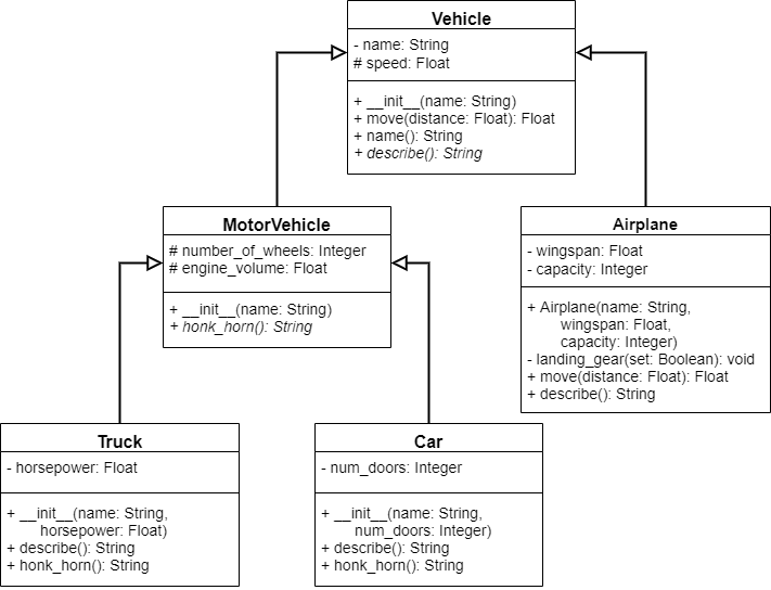
In the UML diagram above, we see that the describe() method in the Vehicle class is printed in italics. That means that the method should be abstract, without any code provided. To do this in Python, we simply inherit from a special class called ABC, short for “Abstract Base Class,” and then use the @abstractmethod decorator:
from abc import ABC, abstractmethod

class Vehicle(ABC):

    def __init__(self, name):
        self.__name = name
        self._speed = 1.0

    @property
    def name(self):
        return self.__name

    def move(self, distance):
        print("Moving");
        return distance / self._speed;

    @abstractmethod
    def describe(self):
        pass
Notice that we must first import both the ABC class and the @abstractmethod decorator from a library helpfully called ABC. Then, we can use ABC as the parent class of our class, and update each method using the @abstractmethod decorator before the method, similar to how we’ve already used @staticmethod in an earlier module.
In addition, since we have declared the method describe() to be abstract, we can either add some code to that method that can be called using super().describe() from a child class, or we can simply choose to use the pass keyword to avoid including any code in the method.
Now, any class that inherits from the Vehicle class must provide an implementation for the describe() method. If it does not, that class must also be declared to be abstract. So, for example, in the UML diagram above, we see that the MotorVehicle class does not include an implementation for describe(), so we’ll also have to make it abstract.
Of course, that means that we’ll have to inherit from both Vehicle and ABC. In Python, we can do that by simply including both classes in parentheses after the subclass name, separated by a comma.
This chapter covered the rest of the programming basics we’ll need to know before starting on the new content of this course. By now we should be pretty familiar with the basic syntax of the language we’ve chosen, as well as the concepts of classes, objects, inheritance, and polymorphism in object-oriented programming. Finally, we’ve explored the Model-View-Controller (MVC) architecture, which will be used extensively in this course.
The big introduction to new content!
One way to look at a computer program is to think of it as a list of instructions that the computer should follow. However, in another sense, many computer programs are simply ways to manipulate data to achieve a desired result. We’ve already written many programs that do this, from calculating the minimum and maximum values of a list of numbers, to storing and retrieving data about students and teachers in a school.
As we start to consider our programs as simply ways to manipulate data, we may quickly realize that we are performing the same actions over and over again, or even treating data in many similar ways. Over time, these ideas have become the basis for several common data structures that we may use in our programs.
Broadly speaking, a data structure is any part of our program that stores data using a particular format or method. Typically data structures define how the data is arranged, how it is added to the structure, how it can be removed, and how it can be accessed.
Data structures can give us very useful ways to look at how our data is organized. In addition, a data structure may greatly impact how easy, or difficult, it can be to perform certain actions with the data. Finally, data structures also impose performance limitations on our code. Some structures may be better at performing a particular operation than others, so we may have to consider that as well when choosing a data structure for our program.
In this class, we’ll spend the majority of our time learning about these common data structures, as well as algorithmic techniques that work well with each one. By formalizing these structures and techniques, we are able to build a common set of building blocks that every programmer is familiar with, making it much easier to build programs that others can understand and reuse.
First, let’s review some of these common data structures and see how they could be useful in our programs.
File:Binary tree.svg. (2019, September 14). Wikimedia Commons, the free media repository. Retrieved 22:18, February 7, 2020 from https://commons.wikimedia.org/w/index.php?title=File:Binary_tree.svg&oldid=365739199. ↩︎

First, we can broadly separate the data structures we’re going to learn about into two types, linear and non-linear data structures.
A linear data structure typically stores data in a single dimension, just like an array. By using a linear data structure, we would know that a particular element in the data structure comes before another element or vice-versa, but that’s about it. A great example is seen in the image above. We have a list of numbers, and each element in the list comes before another element, as indicated by the arrows.
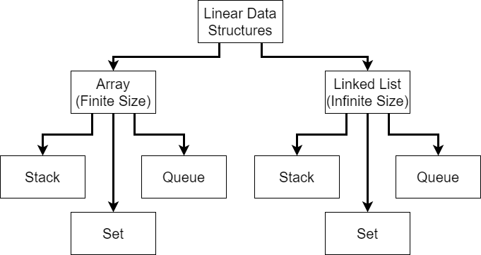
Linear data structures can further be divided into two types: arrays, which are typically finite sized; and linked lists, which can be infinitely sized. We’ve already worked with arrays extensively by this point, but linked lists are most likely a new concept. That’s fine! We’ll explore how to build our own later in this course.
Using either arrays or linked lists, we can build the three most commonly used linear data structures: stacks, queues, and sets. However, before we learn about each of those, let’s review a bit more about what the list data structure itself looks like.
The list data structure is the simplest form of a linear data structure. As we can guess from the definition, a list is simply a grouping of data that is presented in a given order. With lists, not only do the elements in the list matter, but the order matters as well. It’s not simply enough to state that elements $8$, $6$ and $7$ are in the list, but generally we also know that $8$ comes before $6$, which comes before $7$.
We’ve already learned about arrays, which are perfect examples of lists in programming. In fact, Python uses the data type list in the same way most other programming languages use arrays. Other programming languages, such as Java, provide a list data structure through their standard libraries.
One important way to classify data structures is by the operations they can perform on the data. Since a list is the simplest version of a linear data structure, it has several important operations it can perform:
For example, let’s look at the insert operation. Assume we have the list shown in the following diagram:
Then, we decide we’d like to add the element $4$ at index $3$ in this list. So, we can think of this like trying to place the element in the list as shown below:
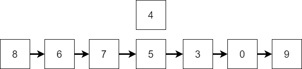
Once we insert that element, we then shift all of the other elements back one position, making the list one element larger. The final version is shown below:

Lists are a very powerful data structure, and one of the most commonly used in a variety of programs. While arrays may seem very flexible, their static size and limited operations can sometimes make them more difficult to use than they are worth. Many programmers choose to use the more flexible list data structure instead.
When deciding which data structure to use, lists are best when we might be adding or removing data from anywhere in the list, but we want to maintain the ordering between elements. As we’ll see on the later pages, we can have more specific types of structures for particular ways we intend to add and remove data from our structure, but lists are a great choice if neither of those are a good fit.
The next two data structures we’ll look at are stacks and queues. They are both very similar to lists in most respects, but each one puts a specific limitation on how the data structure operates that make them very useful in certain situations.
A stack is one special version of a list. Specifically, a stack is a Last In, First Out or LIFO data structure.
So, what does that mean? Basically, we can only add elements to the end, or top of the stack. Then, when we want to get an element from the stack, we can only take the one from the top–the one that was most recently added.
A great way to think of a stack is like a stack of plates, such as the one pictured below:
When we want to add a new plate to the stack, we can just set it on top. Likewise, if we need a plate, we’ll just take the top one off and use it.
A stack supports three major unique operations:
Many stacks also include additional operations such as size and find as well.
A queue is another special version of a list, this time representing a First In, First Out or FIFO data structure.
As seen in the diagram above, new items are added to the back of the queue. But, when we need to take an item from a queue, we’ll take the item that is in the front, which is the one that was added first.
Where have we seen this before? A great example is waiting our turn in line at the train station,
In many parts of the world, the term queueing is commonly used to refer to the act of standing in line. So, it makes perfect sense to use that same word to refer to a data structure.
As we can probably guess, we would definitely want to use a stack if we need our data structure to follow the last in, first out, or LIFO ordering. Similarly, we’d use a queue if we need first in, first out or FIFO ordering.
If we can’t be sure that one or the other of those orderings will work for us, then we can’t really use a stack or a queue in our program.
Of course, one of the biggest questions that comes from this is “why not just use lists for everything?” Indeed, lists can be used as both a queue and a stack, simply by consistently inserting and removing elements from either the beginning or the end of the list as needed. So why do we need to have separate data structures for a queue and a stack?
There are two important reasons. First, if we know that we only need to access the most recently added element, or the element added first, it makes sense to have a special data structure for just that usage. In this way, it is clear to anyone else reading our program that we will only be using the data in that specific way. Behind the scenes, of course, we can just use a list to represent a queue or a stack, but in our design documents and in our code, it might be very helpful to know if we should think of it like a stack or a queue.
The other reason has to do with performance. By knowing exactly how we need to use the data, we can design data structures that are specifically created to perform certain operations very quickly and efficiently. A generic list data structure may not be as fast or memory efficient as a structure specifically designed to be used as a stack, for example.
As we learn about each of these data structures throughout this course, we’ll explore how each data structure works in terms of runtime performance and memory efficiency.
File:Lifo stack.png. (2017, August 7). Wikimedia Commons, the free media repository. Retrieved 23:14, February 7, 2020 from https://commons.wikimedia.org/w/index.php?title=File:Lifo_stack.png&oldid=254596945. ↩︎
File:Tallrik - Ystad-2018.jpg. (2019, December 31). Wikimedia Commons, the free media repository. Retrieved 23:17, February 7, 2020 from https://commons.wikimedia.org/w/index.php?title=File:Tallrik_-_Ystad-2018.jpg&oldid=384552503. ↩︎
File:Data Queue.svg. (2014, August 15). Wikimedia Commons, the free media repository. Retrieved 23:21, February 7, 2020 from https://commons.wikimedia.org/w/index.php?title=File:Data_Queue.svg&oldid=131660203. ↩︎
File:People waiting a train of Line 13 to come 02.JPG. (2016, November 28). Wikimedia Commons, the free media repository. Retrieved 23:23, February 7, 2020 from https://commons.wikimedia.org/w/index.php?title=File:People_waiting_a_train_of_Line_13_to_come_02.JPG&oldid=223382692. ↩︎
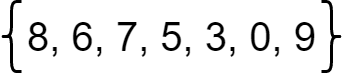
Another linear data structure is known as a set. A set is very similar to a list, but with two major differences:
In fact, the term set comes from mathematics. We’ve probably seen sets already in a math class.
Beyond the typical operations to add and remove elements from a set, there are several operations unique to sets:
Again, many of these operations may be familiar from their use in various math classes.
In addition, we can easily think of set operations as boolean logic operators. For example, the set operation union is very similar to the boolean operator or, as seen in the diagram below.
As long as an item is contained in one set or the other, it is included in the union of the sets.
Similarly, the same comparison works for the set operation intersection and the boolean and operator.
Once again, if an item is contained in the first set and the second set, it is contained in the intersection of those sets.
A set is a great choice when we know that our program should prevent duplicate items from being added to a data structure. Likewise, if we know we’ll be using some of the specific operations that are unique to sets, then a set is an excellent choice.
Of course, if we aren’t sure that our data structure will only store unique items, we won’t be able to use a set.
File:Venn0111.svg. (2019, November 15). Wikimedia Commons, the free media repository. Retrieved 02:37, February 8, 2020 from https://commons.wikimedia.org/w/index.php?title=File:Venn0111.svg&oldid=375571745. ↩︎
File:Venn0001.svg. (2019, November 15). Wikimedia Commons, the free media repository. Retrieved 02:37, February 8, 2020 from https://commons.wikimedia.org/w/index.php?title=File:Venn0001.svg&oldid=375571733. ↩︎
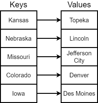
The last of the linear data structures may seem linear from the outside, but inside it can be quite a bit more complex.
The map data structure is an example of a key-value data structure, also known as a dictionary or associative array. In the simplest case, a map data structure keeps track of a key that uniquely identifies a particular value, and stores that value along with the key in the data structure.
Then, to retrieve that value, the program must simply provide the same key that was used to store it.
In a way, this is very similar to how we use an array, since we provide an array index to store and retrieve items from an array. The only difference is that the key in a map can be any data type! So it is a much more powerful data structure.
In fact, this data structure is one of the key ideas behind modern databases, allowing us to store and retrieve database records based on a unique primary key attached to each row in the database.
A map data structure should support the following operations:
Later in this course, we’ll devote an entire module to learning how to build our own map data structures and explore these operations in more detail.
One of the most common ways to implement the map data structure is through the use of a hash table. A hash table uses an array to store the values in the map, and uses a special function called a hash function to convert the given key to a simple number. This number represents the array index for the value. In that way, the same key will always find the value that was given.
But what if we have two keys that produce the same array index? In that case, we’ll have to add some additional logic to our map to handle that situation.
Maps are great data structures when we need to store and retrieve data using a specific key. Just like we would store data in a database or put items in a numbered box to retrieve later, we can use a map as a general purpose storage and retrieval data structure.
Of course, if our data items don’t have unique keys assigned to them, then using a map may not be the best choice of data structure. Likewise, if each key is a sequential integer, we may be able to use an array just as easily.
File:Hash table 3 1 1 0 1 0 0 SP.svg. (2019, August 21). Wikimedia Commons, the free media repository. Retrieved 02:46, February 8, 2020 from https://commons.wikimedia.org/w/index.php?title=File:Hash_table_3_1_1_0_1_0_0_SP.svg&oldid=362787583. ↩︎
The other type of data structure we can use in our programs is the non-linear data structure.
Broadly speaking, non-linear data structures allow us to store data across multiple dimensions, and there may be multiple paths through the data to get from one item to another. In fact, much of the information stored in the data structure has to do with the paths between elements more than the elements themselves.
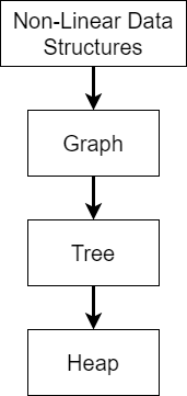
Just like linear data structures, there are several different types of non-linear data structures. In this case, each one is a more specialized version of the previous one, hence the hierarchy shown above. On the next few pages, we’ll explore each one just a bit to see what they look like.
File:6n-graf.svg. (2020, January 12). Wikimedia Commons, the free media repository. Retrieved 02:53, February 8, 2020 from https://commons.wikimedia.org/w/index.php?title=File:6n-graf.svg&oldid=386942400. ↩︎
The most general version of a non-linear data structure is the graph, as shown in the diagram above. A graph is a set of nodes that contain data, as well as a set of edges that link two nodes together. Edges themselves may also contain data.
Graphs are great for storing and visualizing not just data, but also the relationships between data. For example, each node in the graph could represent a city on the map, with the edges representing the travel time between the two cities. Or we could use the nodes in a graph to represent the people in a social network, and the edges represent connections or friendships between two people. There are many possibilities!
Graphs are a great choice when we need to store data and relationships between the data, but we aren’t sure exactly what structures or limitations are present in the data. Since a graph is the most general and flexible non-linear data type, it has the most ability to represent data in a wide variety of ways.
File:Directed acyclic graph 2.svg. (2016, May 3). Wikimedia Commons, the free media repository. Retrieved 03:05, February 8, 2020 from https://commons.wikimedia.org/w/index.php?title=File:Directed_acyclic_graph_2.svg&oldid=195167720. ↩︎
 [^1]
[^1]
File:Tree (computer science).svg. (2019, October 20). Wikimedia Commons, the free media repository. Retrieved 03:13, February 8, 2020 from https://commons.wikimedia.org/w/index.php?title=File:Tree_(computer_science).svg&oldid=371240902.
A tree is a more constrained version of a graph data structure. Specifically, a tree is a graph that can be shown as a hierarchical structure, where each node in the tree is itself the root of a smaller tree. Each node in the tree can have one or more child nodes and exactly one parent node, except for the topmost node or root node, which has no parent nodes.
A tree is very useful for representing data in a hierarchical or sorted format. For example, one common use of a tree data structure is to represent knowledge and decisions that can be made to find particular items. The popular children’s game 20 Questions can be represented as a tree with 20 levels of nodes. Each node represents a particular question that can be asked, and the children of that node represent the possible answers. If the tree only contains yes and no questions, it can still represent up to $2^{20} = 1,408,576$ items!
Another commonly used tree data structure is the trie, which is a special type of tree used to represent textual data. Ever wonder how a computer can store an entire dictionary and quickly spell-check every single word in the language? It actually uses a trie!
Below is a small example of a trie data structure:
This trie contains the words “to”, “tea”, “ted”, “ten”, “i”, “in”, “inn” and “A” in just a few nodes and edges. Imagine creating a trie that could store the entire English language! While it might be large, we can hopefully see how it would be much more efficient to search and store that data in a trie instead of a linear data structure.
A tree is a great choice for a data structure when there is an inherent hierarchy in our data, such that some nodes or elements are naturally “parents” of other elements. Likewise, if we know that each element may only have one parent but many children, a tree becomes an excellent choice. Trees contain several limitations that graphs do not, but they are also very powerful data structures.
File:Trie example.svg. (2014, March 2). Wikimedia Commons, the free media repository. Retrieved 03:22, February 8, 2020 from https://commons.wikimedia.org/w/index.php?title=File:Trie_example.svg&oldid=117843653. ↩︎
The last non-linear data structure we’ll talk about is the heap, which is a specialized version of a tree. In a heap, we try to accomplish a few goals:
If we follow those three guidelines, a heap becomes the most efficient data structure for managing a set of data where we always want to get the maximum or minimum value each time we remove an element. These are typically called priority queues, since we remove items based on their priority instead of the order they entered the queue.
Because of this, heaps are very important in creating efficient algorithms that deal with ordered data.
As discussed above, a heap is an excellent data structure for when we need to store elements and then always be able to quickly retrieve either the smallest or largest element in the data structure. Heaps are a very specific version of a tree that specialize in efficiency over everything else, so they are only really good for a few specific uses.
File:Max-Heap.svg. (2014, December 28). Wikimedia Commons, the free media repository. Retrieved 03:25, February 8, 2020 from https://commons.wikimedia.org/w/index.php?title=File:Max-Heap.svg&oldid=144372033. ↩︎
The other major topic covered in this course is the use of algorithms to manipulate the data stored in our data structures.
An algorithm is best defined as a finite list of specific instructions for performing a task. In the real world, we see algorithms all the time. A recipe for cooking your favorite dish, instructions for how to fix a broken car, or a method for solving a complex mathematical equation can all be considered examples of an algorithm. The flowchart above shows Euclid’s Algorithm for finding the greatest common divisor of two numbers.
In this course, however, we’re going to look specifically at the algorithms and algorithmic techniques that are most commonly used with data structures in computer programming.
An algorithmic technique, sometimes referred to as a methodology or paradigm, is a particular way to design an algorithm. While there are a few commonly used algorithms across different data structures, many times each program may need a unique algorithm, or at least an adaptation of an existing algorithm. to perform its work.
To make these numerous algorithms easier to understand, we can loosely categorize them based on the techniques they use to solve the problem. On the next few pages, we’ll introduce some of the more commonly used algorithmic techniques in this course. Throughout this course, we will learn how to apply many of these techniques when designing algorithms that work with various data structures to accomplish a goal.
File:Euclid flowchart.svg. (2019, January 8). Wikimedia Commons, the free media repository. Retrieved 21:43, February 8, 2020 from https://commons.wikimedia.org/w/index.php?title=File:Euclid_flowchart.svg&oldid=334007111. ↩︎
The first algorithmic technique we’ll use is the brute force technique. This is the algorithmic technique that most of us are most familiar with, even if we don’t realize it.
Simply put, a brute force algorithm will try all possible solutions to the problem, only stopping when it finds one that is the actual solution. A great example of a brute force algorithm in action is plugging in a USB cable. Many times, we will try one way, and if that doesn’t work, flip it over and try the other. Likewise, if we have a large number of keys but are unsure which one fits in a particular lock, we can just try each key until one works. That’s the essence of the brute force approach to algorithmic design.
A great example of a brute force algorithm is finding the closest pair of points in a multidimensional space. This could be as simple as finding the two closest cities on a map, or the two closest stars in a galaxy.
To find the answer, a brute force approach would be to simply calculate the distance between each individual pair of points, and then keep track of the minimum distance found. A pseudocode version of this algorithm would be similar to the following.
MINIMUM = infinity
POINT1 = none
POINT2 = none
loop each POINTA in POINTS
    loop each POINTB in POINTS
        if POINTA != POINTB
            DISTANCE = COMPUTE_DISTANCE(POINTA, POINTB)
            if DISTANCE < MINIMUM
                MINIMUM = DISTANCE
                POINT1 = POINTA
                POINT2 = POINTB
            end if
        end if
    end loop
end loop
Looking at this code, if we have $N$ points, it would take $N^2$ steps to solve the problem! That’s not very efficient, event for a small data set. However, the code itself is really simple, and it is guaranteed to find exactly the best answer, provided we have enough time and a powerful enough computer to run the program.
In the project for this module, we’ll implement a few different brute-force algorithms to solve simple problems. This will help us gain more experience with this particular technique.
File:Closest pair of points.svg. (2018, October 20). Wikimedia Commons, the free media repository. Retrieved 22:29, February 8, 2020 from https://commons.wikimedia.org/w/index.php?title=File:Closest_pair_of_points.svg&oldid=324759130. ↩︎
The next most common algorithmic technique is divide and conquer. A divide and conquer algorithm works just like it sounds. First, it will divide the problem into at least two or more smaller problems, and then it will try to solve each of those problems individually. It might even try to subdivide those smaller problems again and again to finally get to a small enough problem that it is easy to solve.
A great real-world example of using a divide and conquer approach to solving a problem is when we need to look for something that we’ve lost around the house. Instead of trying to search the entire house, we can subdivide the problem into smaller parts by looking in each room separately. Then, within each room, we can even further subdivide the problem by looking at each piece of furniture individually. By reducing the problem’s size and complexity, it becomes easier to search through each individual piece of furniture in the house, either finding our lost object or eliminating that area as the likely location it will be found.

One great example of a divide and conquer algorithm is the binary search algorithm. If we have a list of data that has already been sorted, as seen in the figure above, we can easily find any item in the list using a divide and conquer process.
For example, let’s say we want to find the value $19$ in that list. First, we can look at the item in the middle of the list, which is $23$. Is it our desired number? Unfortunately, it is not. So, we need to figure out how we can use it to divide our input into a smaller problem. Thankfully, we know the list is sorted, so we can use that to our advantage. If our desired number is less than the middle number, we know that it must exist in the first half of the list. Likewise, if it is greater than the middle number, it must be in the second half. In this case, since $19$ is less than $23$, we must only look at the first half of the list.
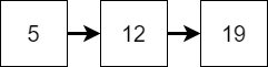
Now we can just repeat that process, this time using only the first half of the original list. This is the powerful feature of a divide and conquer algorithm. Once we’ve figured out how to divide our data, we can usually follow the same steps again to solve the smaller problems as well.
Once again, we ask ourselves if $12$, the centermost number in the list, is the one we are looking for. Once again, it is not, but we know that $19$ is greater than $12$, so we’ll need to look in the second half of the list.

Finally, we have reduced our problem to the simplest, or base case of the problem. Here, we simply need to determine if the single item in the list is the number we are looking for. In this case, it is! So, we can return that our original list did indeed include the number $19$.
We’ll explore many ways of using divide and conquer algorithms in this course, especially when we learn to sort and search through lists of values.
Another algorithmic technique that we’ll learn about is the greedy technique. In a greedy algorithm, the program tries to build a solution one piece at a time. At each step, it will act “greedy” by choosing the piece that it thinks is the best choice for the solution based on the available information. Instead of trying every possible solution like a brute force algorithm or dividing the problem into smaller parts like the divide and conquer approach, a greedy algorithm will just try to construct the one best answer it can.
For example, we can use a greedy algorithm to determine the fewest number of coins needed to give change, as shown in the example above. If the customer is owed $36$ cents, and we have coins worth $20$ cents, $10$ cents, $5$ cents and $1$ cent, how many coins are needed to reach $36$ cents?
In a greedy solution, we could choose the coin with the highest value that is less than the change required, give that to the customer, and subtract its value from the remaining change. In this case, it will indeed produce the optimal solution.
In fact, both the United States dollar and the European euro have a system of coins that will always produce the minimum number of coins with a greedy algorithm. So that’s very helpful!
However, does it always work? What if we have a system that has coins worth $30$ cents, $18$ cents $4$ cents, and $1$ cent. Would a greedy algorithm produce the result with the minimum number of coins when making change for $36$ cents?
Let’s try it and see. First, we see that we can use a $30$ cent coin, leaving us with $6$ cents left. Then, we can use a single $4$ cent coin, as well as two $1$ cent coins for a total of $4$ coins: $30 + 4 + 1 + 1 = 36$.
Is that the minimum number of coins?
It turns out that this system includes a coin worth $18$ cents. So, to make $36$ cents, we really only need $2$ coins: $18 + 18 = 36$!
This is the biggest weakness of the greedy approach to algorithm design. A greedy algorithm will find a possible solution, but it is not guaranteed to be the best possible solution. Sometimes it will work just fine, but other times it may produce solutions that are not very good at all. So we always must consider that when creating an algorithm using a greedy technique.
File:Greedy algorithm 36 cents.svg. (2019, April 27). Wikimedia Commons, the free media repository. Retrieved 23:19, February 8, 2020 from https://commons.wikimedia.org/w/index.php?title=File:Greedy_algorithm_36_cents.svg&oldid=347456702. ↩︎
The next algorithmic technique we’ll discuss is recursion. Recursion is closely related to the divide and conquer method we discussed earlier. However, recursion itself is a very complicated term to understand. It usually presents one of the most difficult challenges for a novice programmer to overcome when learning to write more advanced programs. Don’t worry! We’ll spend an entire module on recursion later in this course.
There are many different ways to define recursion. In one sense, recursion is a problem solving technique where the solution to a problem depends on solutions to smaller versions of the problem, very similar to the divide and conquer approach.
However, to most programmers, the term recursion is used to describe a function or method that calls itself inside of its own code. It may seem strange at first, but there are many instances in programming where a method can actually call itself again to help solve a difficult problem. However, writing recursive programs can be tricky at first, since there are many ways to make simple errors using recursion that cause our programs to break.
Mastering recursion takes quite a bit of time and practice, and nearly every programmer has a strong memory of the first time recursion made sense in their minds. So, it is important to make sure we understand it! In fact, it is so notable, that when we search for “recursion” on Google, it helpfully prompts us if we want to search for “recursion” instead, as seen at the top of this page.
A great example of a recursive method is calculating the factorial of a number. We may recall from mathematics that the factorial of a number is the product of each integer from 1 up to and including that number. For example, the factorial of $5$, written as $5!$, is calculated as $5 * 4 * 3 * 2 * 1 = 120$
We can easily write a traditional method to calculate the factorial of a number as follows.
function ITERATIVE_FACTORIAL(N)
    RESULT = 1
    loop I from 1 to N:
        RESULT = RESULT * I
    end loop
    return RESULT
end function
However, we may also realize that the value of $5!$ is the same as $4! * 5$. If we already know how to find the factorial of $4$, we can just multiply that result by $5$ to find the factorial of $5$. As it turns out, there are many problems in the real world that work just like this, and, in fact, many of the data structures we’ll learn about are built in a similar way.
We can rewrite this iterative function to be a recursive function instead.
function RECURSIVE_FACTORIAL(N)
    if N == 1
        return 1
    else
        return N * RECURSIVE_FACTORIAL(N - 1)
    end if
end function
As we can see, a recursive function includes two important elements, the base case and a recursive case. We need to include the base case so we can stop calling our recursive function over and over again, and actually reach a solution. This is similar to the termination condition of a for loop or while loop. If we forget to include the base case, our program will recurse infinitely!
The second part, the recursive case, is used to reduce the problem to a smaller version of the same problem. In this case, we reduce $N!$ to $N * (N - 1)!$. Then, we can just call our function again to solve the problem $(N - 1)!$, and multiply the result by $N$ to find the solution to $N!$.
So, if we have a problem that can be reduced to a smaller instance of itself, we may be able to use recursion to solve it!
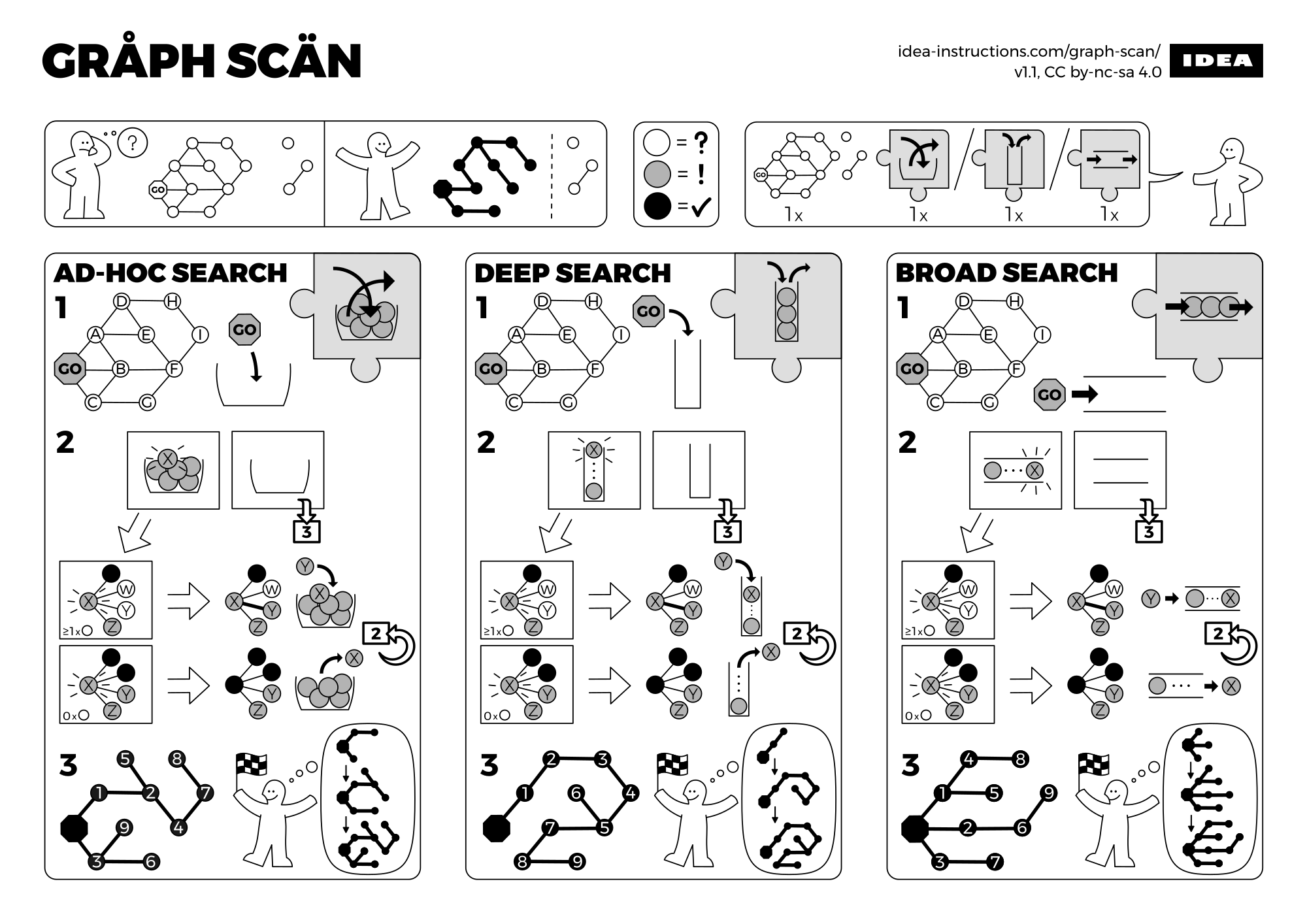
Beyond the algorithmic techniques we’ve introduced so far, there are a number of techniques that deal specifically with data stored in non-linear data structures based on graphs. Generally speaking, we can group all of these algorithms under the heading graph traversal algorithms.
A graph traversal algorithm constructs an answer to a problem by moving between nodes in a graph using the graph’s edges, thereby traversing the graph. For example, a graph traversal algorithm could be used by a mapping program to construct a route from one city to another on a map, or to determine friends in common on a social networking website.
A great example of a graph traversal algorithm is Dijkstra’s Algorithm, which can be used to find the shortest path between two selected nodes in a graph. In the image above, we can see the process of running Dijkstra’s Algorithm on a graph that contains just a few nodes.
Of course, we can use the same approach on any open space, as seen in this animation. Starting at the lower left corner, the algorithm slowly works toward the goal node, but it eventually runs into an obstacle. So, it must find a way around the obstacle while still finding the shortest path to the goal.
Algorithms such as Dijkstra’s Algorithm, and a more refined version called the A* Algorithm are used in many different computer programs to help find a path between two points, especially in video games.
File:Dijkstra Animation.gif. (2018, November 24). Wikimedia Commons, the free media repository. Retrieved 01:45, February 9, 2020 from https://commons.wikimedia.org/w/index.php?title=File:Dijkstra_Animation.gif&oldid=329177321. ↩︎ ↩︎
In this course, we will learn how to develop several different data structures, and then use those data structures in programs that implement several different types of algorithms. However, one of the most difficult parts of programming is clearly explaining what a program should do and how it should perform.
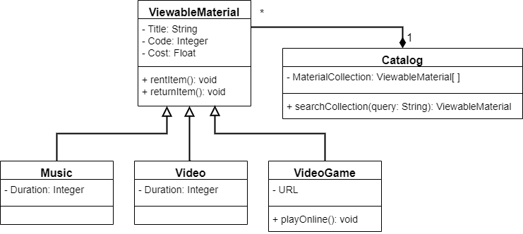
So far, we’ve used UML class diagrams to discuss the structure of a program. It can give us information about the classes, attributes, and methods that our program will contain, as well as the overall relationships between the classes. We can even learn if attributes and methods are private or public, and more.
However, to describe what each method does, we have simply relied on descriptions in plain language up to this point, with no specific format at all. In this module, we’ll introduce the concept of programming by contract to help us provide more specific information about what each method should do and the expectations we can count on based on the inputs and outputs of the method.
Specifically, we’ll learn about the preconditions that are applied to the parameters of a method to make sure they are valid, the postconditions that the method will guarantee if the preconditions are met, and the invariants that a loop or data structure will maintain.
Finally, we can put all of that information together to discuss how to prove that an algorithm correctly performs the task it was meant to, and how to make sure that it works correctly in all possible cases.
First, let’s discuss preconditions. A precondition is an expectation applied to any parameters and existing variables when a method or function is called. Phrased a different way, the preconditions should all be true before the method is called. If all of the preconditions are met, the function can proceed and is expected to function properly. However, if any one of the preconditions are not met, the function may either reach an exception, prompt the user to correct the issue, or produce invalid output, depending on how it is written.
Let’s consider an example method to see how we can define the preconditions applied to that method. In this example, we’re going to write a method triangleArea(side1, side2, side3) that will calculate the area of a triangle, given the lengths of the sides of the triangle.
So, to determine what the preconditions of that method should be, we must think about what we know about a triangle and what sort of data we expect to receive.
For example, we know that the length of each side should be a number. In addition, those lengths should all be positive, so each one must be strictly greater than $0$.
We can also determine if we expect the length to be whole numbers or floating-point numbers. To make this example simpler, let’s just work with whole numbers.
When looking at preconditions, determining the types and expected range of values of each parameter is a major first step. However, sometimes we must also look at the relationship between the parameters to find additional preconditions that we must consider.
For example, the triangle inequality states that the longest side of a triangle must be strictly shorter than the sum of the other two sides. Otherwise, those sides will not create a triangle. So, another precondition must state that the sides satisfy the triangle inequality.
All together, we’ve found the following preconditions for our method triangleArea(side1, side2, side3):
side1, side2 and side3 each must each be an integer that is strictly greater than $0$side1, side2 and side3 must satisfy the triangle inequalityWhat if our method is called and provided a set of parameters that do not meet the preconditions described above? As a programmer, there are several actions we can take in our code to deal with the situation.
One of the most common ways to handle precondition failures is to simply throw or raise exceptions from our method as soon as it determines that the preconditions are not met. In this way, we can quickly indicate that the program is unable to perform the requested operation, and leave it up to the code that called that method to either handle the exception or ignore it and allow the program to crash.
This method is best used within the model portions of a program written using the Model-View-Controller or MVC architecture. By doing so, this allows our controller to react to problems quickly, usually by requesting additional input from the user using the view portion of the program.
In simpler programs, it is common for the code to simply handle the precondition failure by asking the user for new input. This is commonly done in programs that are small enough to fit in a single class, instead of being developed using MVC architecture.
Of course, we could choose to simply ignore these precondition failures and allow our code to continue running. IN that case, if the preconditions are not met, then the answer we receive may be completely invalid. On the next page, we’ll discuss how failed preconditions affect whether we can trust our method’s output.
File:TriangleInequality.svg. (2015, July 10). Wikimedia Commons, the free media repository. Retrieved 23:22, January 21, 2020 from https://commons.wikimedia.org/w/index.php?title=File:TriangleInequality.svg&oldid=165448754. ↩︎
Next, we can discuss postconditions. A postcondition is a statement that is guaranteed to be true after a method is executed, provided all of the preconditions were met. If any one of the preconditions were not met, then we can’t count on the postcondition being true either. This is the most important concept surrounding preconditions and postconditions.
If the preconditions of a method are all true when a method is called, then we may assume the postconditions are true after the method is complete, provided it is written correctly.
On the last page, we discussed the preconditions for a method triangleArea(side1, side2, side3) that will calculate the area of a triangle given the lengths of its sides. Those preconditions are:
side1, side2 and side3 each must each be an integer that is strictly greater than $0$side1, side2 and side3 must satisfy the triangle inequalitySo, once the method completes, what should our postcondition be? In this case, we want to find a statement that would be always true if all of the preconditions are met.
Since the method will be calculating the area of the triangle, the strongest postcondition we can use is the most obvious one:
side1, side2 and side3That’s really it!
Of course, there are a few other postconditions that we could consider, especially when we start working with data structures and objects. For example, one of the most powerful postconditions is the statement:
When we call a method that accepts an array or object as a parameter, we know that we can modify the values stored in that array or object because the parameter is handled in a call-by-reference fashion in most languages. So, if we don’t state that this postcondition applies, we can’t guarantee that the method did not change the values in the array or object we provided as a parameter.
So, what if the preconditions are not met? Then what happens?
As we discussed on the previous page, if the preconditions are not met, then we cannot guarantee that the postcondition will be true once the method executes. In fact, it may be decidedly incorrect, depending on how we implement the method.
For example, the simplest way to find the area of a triangle given the lengths of all three sides is Heron’s formula, which can be written mathematically as:
$$ A = 1/4 \sqrt{(a + b + c)(-a + b + c)(a - b + c)(a + b - c)} $$Since this is a mathematical formula, it is always possible to get a result from it, even if all of the preconditions are not met. For example, the inputs could be floating-point values instead of integers, or they may not satisfy the triangle inequality. In that case, the function may still produce a result, but it will not represent the actual area of the triangle described, mainly because the parameters provided describe a triangle that cannot exist in the real world. So, we must always be careful not to assume that a method will always provide the correct output unless we provide parameters that make all of its preconditions true.
File:Triangle with notations 2 without points.svg. (2018, December 5). Wikimedia Commons, the free media repository. Retrieved 00:03, January 22, 2020 from https://commons.wikimedia.org/w/index.php?title=File:Triangle_with_notations_2_without_points.svg&oldid=330397605. ↩︎
Once we’ve written a program, how can we verify that it works correctly? There are many ways to do this, but one of the most common is unit testing.
Unit testing a program involves writing code that actually runs the program and verifies that it works correctly. In addition, many unit tests will also check that the program produces appropriate errors when given bad input, or even that it won’t crash when given invalid input.
For example, a simple unit test for the maximum() method would be:
function MAXIMUMTEST()
    ARRAY = new array[5]
    ARRAY[0] = 5
    ARRAY[1] = 25
    ARRAY[2] = 10
    ARRAY[3] = 15
    ARRAY[4] = 0
    RESULT = MAXIMUM(ARRAY)
    if RESULT == 25:
        print "Test Passed"
    end if
end function
This code will simply create an array that we know the maximum value of, and then confirm that our own maximum() method will find the correct result.
Of course, this is a very simplistic unit test, and it would take several more unit tests to fully confirm that the maximum() method works completely correctly.
However, it is important to understand how this test relates to the preconditions and postconditions that were established on previous pages. Here, the unit tests creates a variable ARRAY which is an array of at least one numerical value. Therefore, it has met the preconditions for the maximum() method, so we can assume that if maximum() is written correctly, then the postconditions will be true once it is has executed. This is the key assumption behind unit tests.
In this course, you will be asked to build several data structures and implement algorithms that use those data structures. In the assignment descriptions, we may describe these methods using the preconditions and postconditions applied to them. Similarly, we’ll learn about structural invariants of data structures, which help us ensure that your data structures are always valid.
Then, to grade your work, we use an autograder that contains several unit tests. Those unit tests are used to confirm that you code works correctly, and they do so by providing input that either satisfies the preconditions, meaning that the test expects that the postconditions will be true, or by providing invalid input and testing how your code reacts to those situations.
You’ll see these concepts throughout this course, so it is important to be familiar with them now.
In this chapter, we introduced a number of different data structures that we can use in our programs. In addition, we explored several algorithmic techniques we can use to develop algorithms that manipulate these data structures to allow us to solve complex problems in our code.
Throughout the rest of this course, as well as a subsequent course, we’ll explore many of these data structures and techniques in detail. We hope that introducing them all at the same time here will allow us to compare and contrast each one as we learn more about it, while still keeping in mind that there are many different structures and techniques that will be available to us in the future.
Lists, Stacks, Queues, and Double-Ended Queues (Deques)
A stack is a data structure with two main operations that are simple in concept. One is the push operation that lets you put data into the data structure and the other is the pop operation that lets you get data out of the structure.
Why do we call it a stack? Think about a stack of boxes. When you stack boxes, you can do one of two things: put boxes onto the stack and take boxes off of the stack. And here is the key. You can only put boxes on the top of the stack, and you can only take boxes off the top of the stack. That’s how stacks work in programming as well!

A stack is what we call a “Last In First Out”, or LIFO, data structure. That means that when we pop a piece of data off the stack, we get the last piece of data we put on the stack.

So, where do we see stacks in the real world? A great example is repairing an automobile. It is much easier to put a car back together if we put the pieces back on in the reverse order we took them off. Thus, as we take parts off a car, it is highly recommended that we lay them out in a line. Then, when we are ready to put things back together, we can just start at the last piece we took off and work our way back. This operation is exactly how a stack works.
Another example is a stack of chairs. Often in schools or in places that hold different types of events, chairs are stacked in large piles to make moving the chairs easier and to make their storage more efficient. Once again, however, if we are going to put chairs onto the stack or remove chairs from the stack, we are going to have to do it from the top.
How do we implement stacks in code? One way would be to use something we already understand, an array. Remember that arrays allow us to store multiple items, where each entry in the array has a unique index number. This is a great way to implement stacks. We can store items directly in the array and use a special top variable to hold the index of the top of the stack.
The following figure shows how we might implement a stack with an array. First, we define our array myStack to be an array that can hold 10 numbers, with an index of 0 to 9. Then we create a top variable that keeps track of the index at the top of the array.
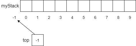
Notice that since we have not put any items onto the stack, we initialize top to be -1. Although this is not a legal index into the array, we can use it to recognize when the stack is empty, and it makes manipulating items in the array much simpler. When we want to push an item onto the stack, we follow a simple procedure as shown below. Of course, since our array has a fixed size, we need to make sure that we don’t try to put an item in a full array. Thus, the precondition is that the array cannot be full. Enforcing this precondition is the function of the if statement at the beginning of the function. If the array is already full, then we’ll throw an exception and let the user handle the situation. Next, we increment the top variable to point to the next available location to store our data. Then it is just a matter of storing the item into the array at the index stored in top.
function PUSH(ITEM)
    if MYSTACK is full then
        throw exception
    end if
    TOP = TOP + 1
    MYSTACK[TOP] = ITEM
end function
If we call the function push(a) and follow the pseudocode above, we will get an array with a stored in myStack[0] and top will have the value 0 as shown below.
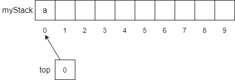
As we push items onto the stack, we continue to increment top and store the items on the stack. The figure below shows how the stack would look if we performed the following push operations.
push("b")
push("c")
push("d")
push("e")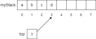
Although we are implementing our stack with an array, we often show stacks vertically instead of horizontally as shown below. In this way the semantics of top makes more sense.
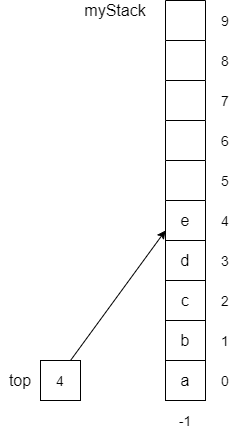
Of course, the next question you might ask is “how do we get items off the stack?”. As discussed above, we have a special operation called pop to take care of that for us. The pseudocode for the pop operation is shown below and is similar in structure to the push operation.
function POP
    if TOP == -1 then
        throw exception
    end if
    TOP = TOP - 1
    return MYSTACK[TOP + 1]
end function
However, instead of checking to see if the stack is full, we need to check if the stack is empty. Thus, our precondition is that the stack is not empty, which we evaluate by checking if top is equal to -1. If it is, we simply throw an exception and let the user handle it. If myStack is not empty, then we can go ahead and perform the pop function. We simply decrement the value of top and return the value stored in myStack[top+1].
Now, if we perform three straight pop operations, we get the following stack.

The following table shows an example of how to use the above operations to create and manipulate a stack. It assumes the steps are performed sequentially and the result of the operation is shown.
| Step | Operation | Effect |
|---|---|---|
| 1 | Constructor | Creates an empty stack. 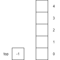
|
| 2 | isFull() |
Returns false since top is not equal to the capacity of the stack.
|
| 3 | isEmpty() |
Returns true since top is equal to -1
|
| 4 | push(1) |
Increments top by 1 and then places item $1$ onto the top of the stack 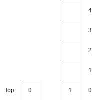
|
| 5 | push(2) |
Increments top by 1 and then places item $2$ onto the top of the stack 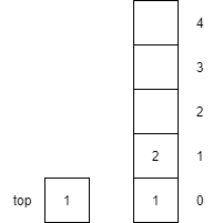
|
| 6 | push(3) |
Increments top by 1 and then places item $3$ onto the top of the stack 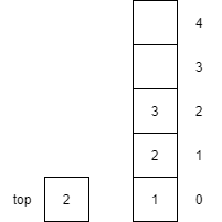
|
| 7 | peek() |
Returns the item $3$ on the top of the stack but does not remove the item from the stack. top is unaffected by peek
|
| 8 | pop() |
Returns the item $3$ from the top of the stack and removes the item from the stack. top is decremented by 1.
|
| 9 | pop() |
Returns the item $2$ from the top of the stack and removes the item from the stack. top is decremented by 1.
|
| 10 | pop() |
Returns the item $1$ from the top of the stack and removes the item from the stack. top is decremented by 1.
|
| 11 | isEmpty() |
Returns true since top is equal to -1
|
Stacks are useful in many applications. Classic real-world software that uses stacks includes the undo feature in a text editor, or the forward and back features of web browsers. In a text editor, each user action is pushed onto the stack as it is performed. Then, if the user wants to undo an action, the text editor simply pops the stack to get the last action performed, and then undoes the action. The redo command can be implemented as a second stack. In this case, when actions are popped from the stack in order to undo them, they are pushed onto the redo stack.
Another example is a maze exploration application. In this application, we are given a maze, a starting location, and an ending location. Our first goal is to find a path from the start location to the end location. Once we’ve arrived at the end location, our goal becomes returning to the start location in the most direct manner.
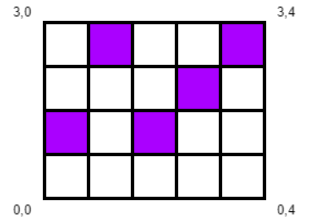
We can do this simply with a stack. We will have to search the maze to find the path from the starting location to the ending location. Each time we take a step forward, we push that move onto a stack. If we run into a dead end, we can simply retrace our steps by popping moves off the list and looking for an alternative path. Once we reach the end state, we will have our path stored in the stack. At this point it becomes easy to follow our path backward by popping each move off the top of the stack and performing it. There is no searching involved.
We start with a maze, a startCell, a goalCell, and a stack as shown below. In this case our startCell is 0,0 and our end goal is 1,1. We will store each location on the stack as we move to that location. We will also keep track of the direction we are headed: up, right, down, or left, which we’ll abbreviate as u,r,d,and l.
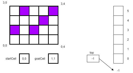
In our first step, we will store our location and direction 0,0,u on the stack.

For the second step, we will try to move “up”, or to location 1,0. However, that square in the maze is blocked. So, we change our direction to r as shown below.
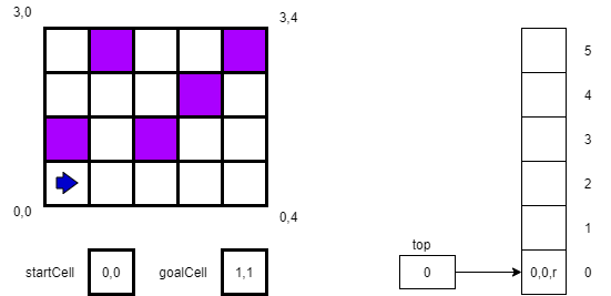
After turning right, we attempt to move in that direction to square 0,1, which is successful. Thus, we create a new location 0,1,u and push it on the stack. (Here we always assume we point up when we enter a new square.) The new state of the maze and our stack are shown below.
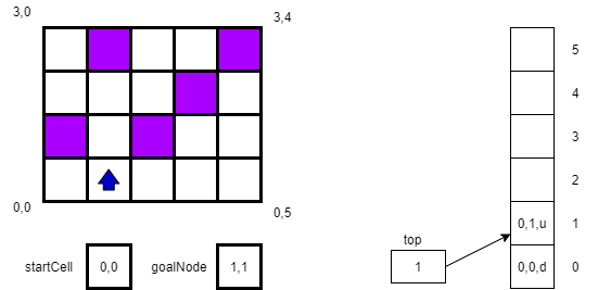
Next, we try to move to 1,1, which again is successful. We again push our new location 1,1,u onto the stack. And, since our current location matches our goalCell location (ignoring the direction indicator) we recognize that we have reached our goal.
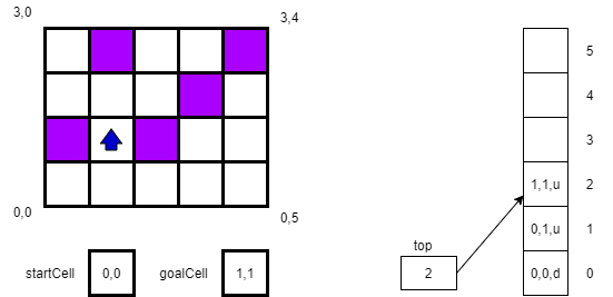
Of course, it’s one thing to find our goal cell, but it’s another thing to get back to our starting position. However, we already know the path back given our wise choice of data structures. Since we stored the path in a stack, we can now simply reverse our path and move back to the start cell. All we need to do is pop the top location off of the stack and move to that location over and over again until the stack is empty. The pseudocode for following the path back home is simple.
loop while !MYSTACK.ISEMPTY()
	NEXTLOCATION = MYSTACK.POP()
	MOVETO(NEXTLOCATION)
end while
The pseudocode for finding the initial path using the stack is shown below. We assume the enclosing class has already defined a stack called myStack and the datatype called Cell, which represents the squares in the maze. The algorithm also uses three helper functions as described below:
getNextCell(maze, topCell): computes the next cell based on our current cell’s location and direction;incrementDirection(topCell): increments a cell’s direction attribute following the clockwise sequence of up, right, down, left, and then finally done, which means that we’ve tried all directions; andvalid(nextCell): determines if a cell is valid. A cell is invalid if it is “blocked”, is outside the boundaries of the maze, or is in the current path (i.e., if it exists in the stack).The parameters of findPath are a 2-dimensional array called maze, the startCell and the endCell. The algorithm begins by pushing the startCell onto myStack. The cell at the top of the stack will always represent our current cell, while the remaining cells in the stack represent the path of cells taken to reach the current cell.
Next, we enter a loop, where we will do the bulk of the work. We peek at the cell on the top of the stack in order to use it in our computations. If the topCell is equal to our goalCell, then we are done and return true indicating that we have found a path to the goal.
If we are not at our goal, we check to see if we have searched all directions from the current cell. If that is the case, then the direction attribute of the topCell will have been set to done. If the direction attribute of topCell is equal to done, then we pop the topCell of the stack, effectively leaving that cell and returning to the next cell in the stack. This is an algorithmic technique called backtracking.
function FINDPATH(MAZE, STARTCELL, GOALCELL)
    MYSTACK.PUSH(STARTCELL);
	loop while !MYSTACK.ISEMPTY()
        TOPCELL = MYSTACK.PEEK()
		if TOPCELL equals GOALCELL
			return true
		if TOPCELL.GETDIRECTION() = done then
            MYSTACK.POP()
		else
            NEXTCELL = GETNEXTCELL(MAZE, TOPCELL)
            INCREMENTDIRECTION(TOPCELL)
			if VALID(MAZE, NEXTCELL) then
				if MYSTACK.ISFULL() then
                    MYSTACK.DOUBLECAPACITY();
				end if
                MYSTACK.PUSH(NEXTCELL)
			end if
		end if
	end while
	return false
end function
However, if we have not searched in all directions from topCell, we will try to explore a new cell (nextCell) adjacent to the topCell. Specifically, nextCell will be the adjacent cell in the direction stored by the direction attribute. We then increment the direction attribute of the topCell so if we end up backtracking, we will know which direction to try next.
Before we push the nextCell onto the stack, we must first check to see if it’s a valid cell by calling the helper function valid. A cell is valid if it is open to be explored. A cell is invalid if it is “blocked,” is outside the boundaries of the maze, or is in the current path (i.e., if it exists in the stack). To help us determine if a cell is in the stack, we will need to extend our stack operations to include a find operation that searches the stack while leaving its contents intact. You will get to implement this operation in your project.
If nextCell is valid, we then check to make sure that the stack is not already full. If it is, we simply call doubleCapacity and continue on our way. Then we push nextCell onto myStack so it will become our next topCell on the next pass through the loop.
After we have explored all possible paths through the maze, the loop will eventually end, and the operation will return false indicating no path was found. While this is not the most efficient path finding algorithm, it is a good example of using stacks for backtracking. Also, if we do find a path and return, the path will be saved in the stack. We can then use the previous pseudocode for retracing our steps and going back to the startCell.
A queue (pronounced like the letter “q”) data structure organizes data in a First In, First Out (FIFO) order: the first piece of data put into the queue is the first piece of data available to remove from the queue. A queue functions just like the line you would get into to go into a ballgame, movie, or concert: the person that arrives first is the first to get into the venue.
You might be thinking that this sounds a lot like the stack structure we studied a few modules back, with the exception that the stack was a Last in, First Out (LIFO) structure. If so, you are correct. The real difference between a stack and a queue is how we take data out of the data structure. In a stack, we put data onto the top of the stack and removed it from the top as well. With a queue, we put data onto the end (or rear) of the queue and remove it from the start (or front) of the queue.
The name for queues comes the word in British English used to describe a line of people. Instead of forming lines to wait for some service, British form queues. Thus, when we think of queues, often the first picture to come to mind is a group of people standing in a line. Of course, this is exactly how a computer queue operates as well. The first person in line gets served first. If I get into line before you do, then I will be served before you do.
Of course, there are other examples of queues besides lines of people. You can think of a train as a long line of railway cars. They are all connected and move together as the train engine pulls them. A line of cars waiting to go through a toll booth or to cross a border is another good example of a queue. The first car in line will be the first car to get through the toll booth. In the picture below, there are actually several lines.
File:BNSF GE Dash-9 C44-9W Kennewick - Wishram WA.jpg. (2019, July 1). Wikimedia Commons, the free media repository. Retrieved 19:30, March 30, 2020 from https://commons.wikimedia.org/w/index.php?title=File:BNSF_GE_Dash-9_C44-9W_Kennewick_-_Wishram_WA.jpg&oldid=356754103. ↩︎
File:El Paso Ysleta Port of Entry.jpg. (2018, April 9). Wikimedia Commons, the free media repository. Retrieved 19:30, March 30, 2020 from https://commons.wikimedia.org/w/index.php?title=File:El_Paso_Ysleta_Port_of_Entry.jpg&oldid=296388002. ↩︎
How do we implement queues in code? Like we did with stacks, we will use an array, which is an easily understandable way to implement queues. We will store data directly in the array and use special start and end variables to keep track of the start of the queue and the end of the queue.
The following figure shows how we might implement a queue with an array. First, we define our array myQueue to be an array that can hold 10 numbers, with an index of 0 to 9. Then we create a start variable to keep track of the index at the start of the queue and an end variable to keep track of the end of the array.

Notice that since we have not put any items into the queue, we initialize start to be -1. Although this is not a legal index into the array, we can use it like we did with stacks to recognize when we have not yet put anything into the queue. As we will see, this also makes manipulating items in the array much simpler. However, to make our use of the array more efficient, -1 will not always indicate that the queue is empty. We will allow the queue to wrap around the array from the start index to the end index. We’ll see an example of this behavior later.
When we want to enqueue an item into the queue, we follow the simple procedure as shown below. Of course, since our array has a fixed size, we need to make sure that we don’t try to put an item in a full array. Thus, the precondition is that the array cannot be full. Enforcing this precondition is the function of the if statement at line 2. If the array is already full, then we’ll throw an exception in line 3 and let the caller handle the situation. Next, we store item at the end location and then compute the new value of end in line 5. Line 6 uses the modulo operator % to return the remainder of the division of $(\text{end} + 1) / \text{length of myQueue}$. In our example, this is helpful when we get to the end of our ten-element array. If end == 9 before enqueue was called, the function would store item in myQueue[9] and then line 4 would cause end to be $(9 +1) % 10$ or $10 % 10$ which is simply $0$, essentially wrapping the queue around the end of the array and continuing it at the beginning of the array.
 1function ENQUEUE (item)
 2  if ISFULL() then
 3    raise exception
 4  end if
 5  MYQUEUE[END] = ITEM
 6  END = (END + 1) % length of MYQUEUE
 7  if START == -1
 8    START = 0
 9  end if
10end function
Given our initial configuration above, if we performed an enqueue(7) function call, the result would look like the following.
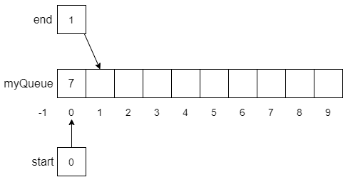
Notice that the value 7 was stored at myQueue[0] in line 5, end was updated to 1 in line 6, and start was set to 0 in line 8. Now, let’s assume we continue to perform enqueue operations until myQueue is almost filled as shown below.
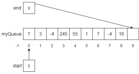
If at this point, we enqueue another number, say -35, the modulo operator in line 6 would help us wrap the end of the list around the array and back to the beginning as expected. The result of this function call is shown below.

Now we have a problem! The array is full of numbers and if we try to enqueue another number, the enqueue function will raise an exception in line 3. However, this example also gives us insight into what the isFull condition should be. Notice that both start, and end are pointing at the same array index. You may want to think about this a little, but you should be able to convince yourself that whenever start == end we will be in a situation like the one above where the array is full, and we cannot safely enqueue another number.
To rectify our situation, we need to have a function to take things out of the queue. We call this function dequeue, which returns the item at the beginning of the queue (pointed at by start) and updates the value of start to point to the next location in the queue. The pseudocode for the dequeue is shown below.
 1function DEQUEUE ()
 2  if ISEMPTY() then
 3    raise exception
 4  end if
 5  ITEM = MYQUEUE[START]
 6  START = (START + 1) % length of MYQUEUE
 7  if START == END
 8    START = -1
 9    END = 0
10  end if
11  return ITEM
12end function
Line 2 checks if the queue is empty and raises an exception in line 3 if it is. Otherwise, we copy the item at the start location into item at line 5 and then increment the value of start by 1, using the modulo operator to wrap to the beginning of the array if needed in line 6. However, if we dequeue the last item in the queue, we will actually run into the same situation that we ran into in the enqueue when we filled the array, start == end. Since we need to differentiate between being full or empty (it’s kind of important!), we reset the start and end values back to their initial state when we dequeue the last item in the queue. That is, we set start = -1 and end = 0. This way, we will always be able to tell the difference between the queue being empty or full. Finally, we return the item to the calling function in line 11.
The following table shows an example of how to use the above operations to create and manipulate a queue. It assumes the steps are performed sequentially and the result of the operation is shown.
| Step | Operation | Effect |
|---|---|---|
| 1 | Constructor | Creates an empty queue of capacity 3. 
|
| 2 | isFull() |
Returns false since start is not equal to end
|
| 3 | isEmpty() |
Returns true since start is equal to -1.
|
| 4 | enqueue(1) |
Places item 1 onto queue at the end and increments end by 1. 
|
| 5 | enqueue(2) |
Places item 2 onto queue at the end and increments end by 1. 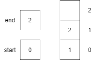
|
| 6 | enqueue(3) |
Places item 3 onto queue at the end and sets end to end+1 modulo the size of the array (3). The result of the operation is 0, thus end is set to 0. 
|
| 7 | peek() |
Returns the item 1 on the start of the queue but does not remove the item from the queue. start and end are unaffected by peek.
|
| 8 | isFull() |
Returns true since start is equal to end
|
| 9 | dequeue() |
Returns the item 1 from the start of the queue. start is incremented by 1, effectively removing 1 from the queue. 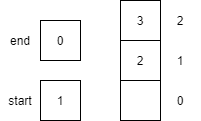
|
| 10 | dequeue() |
Returns the item 2 from the start of the queue. start is incremented by 1, effectively removing 2 from the queue. 
|
| 11 | enqueue(4) |
Places item 4 onto queue at the end and increments end. 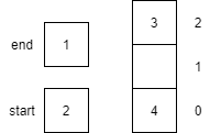
|
| 12 | dequeue() |
Returns the item 3 from the start of the queue. start is set to start+1 modulo the size of the array (3). The result of the operation is 0, thus start is set to 0. 
|
| 13 | dequeue() |
Returns the item 4 from the start of the queue. start is incremented by 1, and since start == end, they are both reset to -1 and 0 respectively.
|
| 14 | isEmpty() |
Returns true since start is equal to -1.
|
Queues are useful in many applications. Classic real-world software which uses queues includes the scheduling of tasks, sharing of resources, and processing of messages in the proper order. A common need is to schedule tasks to be executed based on their priority. This type of scheduling can be done in a computer or on an assembly line floor, but the basic concept is the same.
Let’s assume that we are putting windshields onto new cars in a production line. In addition, there are some cars that we want to rush through production faster than others. There are actually three different priorities:
Ideally, as cars come to the windshield station, we would be able to put their windshields in and send them to the next station before we received the next car. However, this is rarely the case. Since putting on windshields often requires special attention, cars tend to line up to get their windows installed. This is when their priority comes into account. Instead of using a simple queue to line cars up first-come, first-served in FIFO order, we would like to jump high priority cars to the head of the line.
While we could build a sophisticated queueing mechanism that would automatically insert cars in the appropriate order based on priority and then arrival time, we could also use a queue to handle each set of car priorities. A figure illustrating this situation is shown below. As cars come in, they are put in one of three queues: high priority, medium priority, or low priority. When the windshield station completes a car it then takes the next car from the highest priority queue.
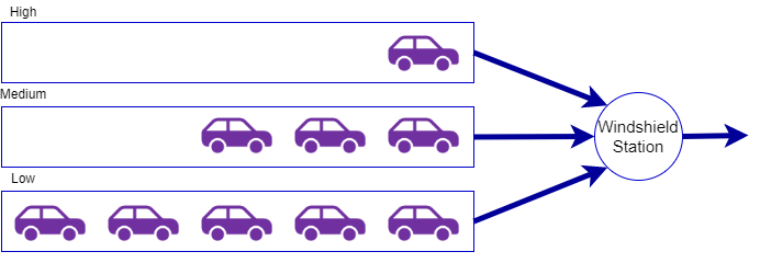
The interesting part of the problem is the controller at the windshield station that determines which car will be selected to be worked on next. The controller will need to have the following interface:
function receiveCar(car, priority)
 // receives a car from the previous station and places into a specific queue

function bool isEmpty()
 // returns true if there are no more cars in the queue

function getCar() returns car
 // retrieves the next car based on priority
Using this simple interface, we will define a class to act as the windshield station controller. It will receive cars from the previous station and get cars for the windshield station.
We start by defining the internal attributes and constructor for the Controller class as follows, using the Queue functions defined earlier in this module. We first declare three separate queues, one each for high, medium, and low priority cars. Next, we create the constructor for the Controller class. The constructor simply initializes our three queues with varying capacities based on the expected usage of each of the queues. Notice, that the high priority queue has the smallest capacity while the low priority queue has the largest capacity.
class Controller
    declare HIGH as a Queue
    declare MEDIUM as a Queue
    declare LOW as a Queue

    function Controller()
        HIGH = new Queue(4)
        MEDIUM = new Queue(6)
        LOW = new Queue(8)
    end function
Next, we need to define the interface function as defined above. We start with the receiveCar function. There are three cases based on the priority of the car. If we look at the first case for priority == high, we check to see if the high queue is full before calling the enqueue function to place the car into the high queue. If the queue is full, we raise an exception. We follow the exact same logic for the medium and low priority cars as well. Finally, there is a final else that captures the case where the user did not specific either high, medium, or low priority. In this case, an exception is raised.
function receiveCar(CAR, PRIORITY)
    if PRIORITY == high
        if HIGH.isFull()
            raise exception
        else
            HIGH.enqueue(CAR)
        end if
    else PRIORITY == medium
        if MEDIUM.isFull()
            raise exception
        else
            MEDIUM.enqueue(CAR)
        end if
    else PRIORITY == low
        if LOW.isFull()
            raise exception
        else
            LOW.enqueue(CAR)
        end if
    else
        raise exception
    end if
end function
Now we will define the isEmpty function. While we do not include an isFull function due to the ambiguity of what that would mean and how it might be useful, the isEmpty function will be useful for the windshield station to check before they request another call via the getCar function.
As you can see below, the isEmpty function simply returns the logical AND of each of the individual queue’s isEmpty status. Thus, the function will return true if, and only if, each of the high, medium, and low queues are empty.
function isEmpty()
    return HIGH.isEmpty() and MEDIUM.isEmpty() and LOW.isEmpty()
end function
Finally, we are able to define the getCar function. It is similar in structure to the receiveCar function in that it checks each queue individually. In the case of getCar, the key to the priority mechanism we are developing is in the order we check the queues. In this case, we check them in the expected order from high to low. If the high queue is not empty, we get the car from that queue and return it to the calling function. If the high queue is empty, then we check the medium queue. Likewise, if the medium queue is empty, we check the low queue. Finally, if all of the queues are empty, we raise an exception.
function getCar()
    if not HIGH.isEmpty()
        return HIGH.dequeue()
    else not MEDIUM.isEmpty()
        return MEDIUM.dequeue()
    else not LOW.isEmpty()
        return LOW.dequeue()
    else
        raise exception
    end if
end functionThe following example shows how the Controller class would work, given specific calls to receiveCar and getCar.
| Step | Operation | Effect |
|---|---|---|
| 1 | Constructor | Creates 3 priority queues. 
|
| 2 | getCar() |
Raises an exception since all three queues will be empty.
|
| 3 | receiveCar(a, low) |
Places car a into the low queue. 
|
| 4 | receiveCar(b, low) |
Places car b into the low queue. 
|
| 5 | receiveCar(f, high) |
Places car f into the high queue. 
|
| 6 | receiveCar(d, medium) |
Places car d into the medium queue. 
|
| 7 | receiveCar(g, high) |
Raises an exception since the high queue is already full.
|
| 8 | receiveCar(e, medium) |
Places car e into the medium queue. 
|
| 9 | getCar() |
Returns car f from the high queue. 
|
| 10 | getCar() |
Returns car d from the medium queue. 
|
| 11 | getCar() |
Returns car e from the medium queue. 
|
| 12 | getCar() |
Returns car a from the low queue. 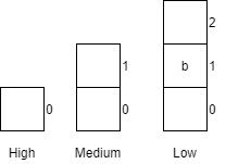
|
| 13 | getCar() |
Returns car b from the low queue.
|
| 14 | getCar() |
Raises an exception since there are no more cars available in any of the three queues.
|
| 15 | isEmpty() |
Returns true since all three queues are empty.
|
A list is a data structure that holds a sequence of data, such as the shopping list shown below. Each list has a head item and a tail item, with all other items placed linearly between the head and the tail. As we pick up items in the store, we will remove them, or cross them off the list. Likewise, if we get a text from our housemate to get some cookies, we can add them to the list as well.
Lists are actually very general structures that we can use for a variety of purposes. One common example is the history section of a web browser. The web browser actually creates a list of past web pages we have visited, and each time we visit a new web page it is added to the list. That way, when we check our history, we can see all the web pages we have visited recently in the order we visited them. The list also allows us to scroll through the list and select one to revisit or select another one to remove from the history altogether.
Of course, we have already seen several instances of lists so far in programming, including arrays, stacks, and queues. However, lists are much more flexible than the arrays, stacks, and queues we have studied so far. Lists allow us to add or remove items from the head, tail, or anywhere in between. We will see how we can actually implement stacks and queues using lists later in this module.
Most of us see and use lists every day. We have a list for shopping as we saw above, but we may also have a “to do” list, a list of homework assignments, or a list of movies we want to watch. Some of us are list-makers and some are not, but we all know a list when we see it.
However, there are other lists in the real world that we might not even think of as a list. For instance, a playlist on our favorite music app is an example of a list. A music app lets us move forward or backward in a list or choose a song randomly from a list. We can even reorder our list whenever we want.
All the examples we’ve seen for stacks and queues can be thought of as lists as well. Stacks of chairs or moving boxes, railroad trains, and cars going through a tollbooth are all examples of special types of lists.
To this point, we have been using arrays as our underlying data structures for implementing linear data structures such as stacks and queues. Given that with stacks and queues we only put items into the array and remove from either the start or end of the data structure, we have been able to make arrays work. However, there are some drawbacks to using arrays for stacks and queues as well as for more general data structures.
While drawbacks 1 and 2 above can be overcome (albeit rather awkwardly) when using arrays for stacks and queues, drawback 3 becomes a real problem when trying to use more general list structures. If we insert an item into the middle of an array, we must move several other items “down” the array to make room.
If for example, if we want to insert the number 5 into the sorted array shown below, we have to carry out several steps:
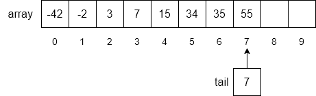
i,i to the end of the list down one place location in the array,i, andIn our example, step 1 will loop through each item of the array until we find the first number in the array greater than 5. As shown below, the number 7 is found in index 3.
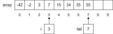
Next, we will use another loop to move each item from index i to the end of the array down by one index number as shown below.
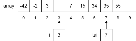
Finally, we will insert our new number, 5, into the array at index 3 and increment tail to 8.
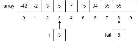
In this operation, if we have $N$ items, we either compare or move all of them, which would require $N$ operations. Of course, this operation runs in order $N$ time.
The same problem occurs when we remove an item from the array. In this case we must perform the following steps:
Instead of using arrays to try to hold our lists, a more flexible approach is to build our own list data structure that relies on a set of objects that are all linked together through references to each other. In the figure below we have created a list of numbers that are linked to each other. Each object contains both the number as well as a reference to the next number in the list. Using this structure, we can search through each item in the list by starting sequentially from the beginning and performing a linear search much like we did with arrays. However, instead of explicitly keeping track of the end of the list, we use the convention that the reference in the last item of the list is set to 0, which we call null. If a reference is set to null we interpret this to mean that there is no next item in the list. This “linked list” structure also makes inserting items into the middle of the list easier. All we need to do is find the location in the list where we want to insert the item and then adjust the references to include the new item into the list.

The following figure shows a slightly more complex version of a linked list, called a “doubly linked list”. Instead of just having each item in the list reference the next item, it references the previous item in the list as well. The main advantage of doubly linked lists is that we can easily traverse the list in either the forward or backward direction. Doubly linked lists are useful in applications to implement undo and redo functions, and in web browser histories where we want the ability to go forward and backward in the history.

We will investigate each of these approaches in more detail below and will reimplement both our stack and queue operations using linked lists instead of arrays.
The content for singly-linked lists has been removed to shorten this chapter. Based on the discussion of doubly-linked lists below, you can probably figure out what a singly-linked list does.
With singly linked lists, each node in the list had a pointer to the next node in the list. This structure allowed us to grow and shrink the list as needed and gave us the ability to insert and delete nodes at the front, middle, or end of the list. However, we often had to use two pointers when manipulating the list to allow us to access the previous node in the list as well as the current node. One way to solve this problem and make our list even more flexible is to allow a node to point at both the previous node in the list as well as the next node in the list. We call this a doubly linked list.
The concept of a doubly linked list is shown below. Here, each node in the list has a link to the next node and a link to the previous node. If there is no previous or next node, we set the pointers to null.
A doubly linked list node is the same as a singly linked list node with the addition of the previous attribute that points to the previous node in the list as shown below.
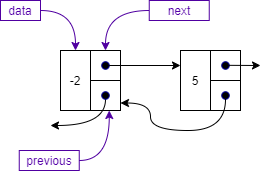
The class representation of a doubly linked list Node is shown below. As discussed above, we have three attributes:
data, which holds the data of the node,next, which is a pointer to the next node, andprevious, which is a pointer to the previous node.We also use a constructor and the standard toString operation to create a string for the data stored in the node.
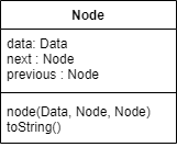
As with our singly linked list, we start off a doubly linked list with a pointer to the first node in the list, which we call head. However, if we also store the pointer to the last node in the list, we can simplify some of our insertion and removal operations as well as reduce the time complexity of operations that insert, remove, or peek at the last node in the list.
The figure below shows a doubly linked list with five nodes. The variable head points to the first node in the list, while the variable tail points to the last node in the list. Each node in the list now has two pointers, next and previous, which point to the appropriate node in the list. Notice that the first node’s previous pointer is null, while the last node’s next pointer is also null.

Like we did for our singly linked list, we capture the necessary details for our doubly linked list in a class. The doubly linked list class has four attributes:
head—the pointer to the first node in the list,tail—the pointer to the last node in the list,current—the pointer to the current node used by the iterator, andsize—an integer to keep track of the number of items in the list.Class DoubleLinkedList
Node head
Node tail
Node current
Integer size = 0You will not be asked to implement a list iterator, but it is an interesting concept to study. Most languages that have a foreach loop construct use iterators behind the scenes to keep track of the current position in the list. This is also why you should not modify the structure of the list while iterating through it using a foreach loop.
An iterator is a set of operations a data structure provides to allow users to access the items in the data structure sequentially, without requiring them to know its underlying representation. There are many reasons users might want to access the data in a list. For instance, users may want to make a copy of their list or count the number of times a piece of data was stored in the list. Or, the user might want to delete all data from a list that matches a certain specification. All of these can be handled by the user using an iterator.
At a minimum, iterators have two operations: reset and getNext. Both of these operations use the list class’s current attribute to keep track of the iterator’s current node.
The reset operation initializes or reinitializes the current pointer. It is typically used to ensure that the iterator starts at the beginning of the list. All that is required is for the current attribute be set to null.
function reset()
  current = null
end functionThe main operation of the iterator is the getNext operation. Basically, the getNext operation returns the next available node in the list if one is available. It returns null if the list is empty or if current is pointing at the last node in the list.
Lines 2 and 3 in the getNext operation check to see if we have an empty list, which results in returning the null value. If we have something in the list but current is null, this indicates that the reset operation has just been executed and we should return the data in the first node. Therefore, we set current = head in line 6. Otherwise, we set the current pointer to point to the next node in the list in line 8.
 1function getNext() returns data
 2  if isEmpty()
 3    return null
 4  end if
 5  if current == null
 6    current = head
 7  else
 8    current = current.next
 9  end if
10  if current == null
11    return null
12  else
13    return current.data
14  end if
15end function
Next we return the appropriate data. If current == null we are at the end of the list and so we return the null value in line 11. If current is not equal to null, then it is pointing at a node in the list, so we simply return current.data in line 13.
While not technically part of the basic iterator interface, the removeCurrent operation is an example of operations that can be provided to work hand-in-hand with a list iterator. The removeCurrent operation allows the user to utilize the iterator operations to find a specific piece of data in the list and then remove that data from the list. Other operations that might be provided include being able to replace the data in the current node, or even insert a new piece of data before or after the current node.
The removeCurrent operation starts by checking to make sure that current is really pointing at a node. If it is not, then the condition is caught in line 2 and an exception is raised in line 3. Next, we set the next pointer in the previous node to point to the current node’s next pointer in lines 5 - 9, taking into account whether the current node is the first node in the list. After that, we set the next node’s previous pointer to point back at the previous node in line 10 - 14, considering whether the node is the last node in the list. Finally, we decrement size in line 15.
function removeCurrent()
  if current == null
    raise exception
  end if
  if current.previous != null
    current.previous.next = current.next
  else
    head = current.next
  end
  if current.next != null
    current.next.previous = current.previous
  else
    tail = current.previous
  end if
    current = current.previous
  size – size – 1
end functionThere are several applications for list iterators. For our example, we will use the case where we need a function to delete all instances of data in the list that match a given piece of data. Our deleteAll function resides outside the list class, so we will have to pass in the list we want to delete the data from.
We start the operation by initializing the list iterator in line 2, followed by getting the first piece of data in the list in line 3. Next, we’ll enter a while loop and stay in that loop as long as our copy of the current node in the list, listData, is not null. When it becomes null, we are at the end of the list and we can exit the loop and the function.
function deleteAll(list, data)
  list.reset()
  listData = list.getNext()
  while listData != null
    if listData == data
      list.removeCurrent()
    end if
    listData = list.getNext()
  end while
end function
Once in the list, it’s a matter of checking if our listData is equal to the data we are trying to match. If it is, we call the list’s removeCurrent operation. Then, at the bottom of the list, we get the next piece of data from the list using the list iterator’s getNext operation.
By using a list iterator and a limited set of operations on the current data in the list, we can allow list users to manipulate the list while ensuring that the integrity of the list remains intact. Since we do not know ahead of time how a list will be used in a given application, an iterator with associated operations can allow the user to use the list in application-specific ways without having to add new operations to the list data structure.
Implementing a queue with a doubly linked list is straightforward and efficient. The core queue operations (enqueue, dequeue, isEmpty, and peek) can all be implemented by directly calling list operations that run in constant time. The only other major operation is the toString operation, which is also implemented by directly calling the list toString operation; however, it runs in order $N$ time due to the fact that the list toString operation must iterate through each item in the list.
The key queue operations and their list-based implementations are shown below.
| Operation | Implementation |
|---|---|
enqueue |
|
dequeue |
|
isEmpty |
|
peek |
|
toString |
|
Stacks can be implemented using a similar method - namely adding and removing from the end of the list. This can even be done using a singly-linked list, and is very efficient.
In this module we looked at the stack data structure. Stacks are a “last in first out” data structure that use two main operations, push and pop, to put data onto the stack and to remove data off of the stack. Stacks are useful in many applications including text editor “undo” and web browser “back” functions.
We also saw the queue data structure. Queues are a “first in first out” data structure that use two main operations, enqueue and dequeue, to put data into the queue and to remove data from the queue. Queues are useful in many applications including the scheduling of tasks, sharing of resources, and processing of messages in the proper order.
Finally, we introduced the concept of a linked list, discussing both singly and doubly linked lists. Both kinds of lists are made up of nodes that hold data as well as references (also known as pointers) to other nodes in the list. Singly linked lists use only a single pointer, next, to connect each node to the next node in the list. While simple, we saw that a singly linked list allowed us to efficiently implement a stack without any artificial bounds on the number of items in the list.
With doubly linked lists, we added a previous pointer that points to the previous node. This makes the list more flexible and makes it easier to insert and remove nodes from the list. We also added a tail pointer to the class, which keeps track of the last node in the list. The tail pointer significantly increased the efficiency of working with nodes at the end of the list. Adding the tail pointer allowed us to implement all the major queue operations in constant time.
def: recursion (noun) - see recursion
We are now used to using functions in our programs that allow us to decompose complex problems into smaller problems that are easier to solve. Now, we will look at a slight wrinkle in how we use functions. Instead of simply having functions call other functions, we now allow for the fact that a function can actually call itself! When a function calls itself, we call it recursion.
Using recursion often allows us to solve complex problems elegantly—with only a few lines of code. Recursion is an alternative to using loops and, theoretically, any function that can be solved with loops can be solved with recursion and vice versa.
So why would a function want to call itself? When we use recursive functions, we are typically trying to break the problem down into smaller versions of itself. For example, suppose we want to check to see if a word is a palindrome (i.e., it is spelled the same way forwards and backwards). How would we do this recursively? Typically, we would check to see if the first and last characters were the same. If so, we would check the rest of the word between the first and last characters. We would do this over and over until we got down to the 0 or 1 characters in the middle of the word. Let’s look at what this might look like in pseudocode.
function isPalindrome (String S) returns Boolean
    if length of S < 2 then
        return true
    else
        return (first character in S == last character in S) and
                isPalindrome(substring of S without first and last character)
    end if
end function
First, we’ll look at the else part of the if statement. Essentially, this statement determines if the first and last characters of S match, and then calls itself recursively to check the rest of the word S. Of course, if the first and last characters of S match and the rest of the string is a palindrome, the function will return true. However, we can’t keep calling isPalindrome recursively forever. At some point we have to stop. That is what the if part of the statement does. We call this our base case. When we get to the point where the length of the string we are checking is 0 or 1 (i.e., < 2), we know we have reached the middle of the word. Since all strings of length 0 or 1 are, by definition, palindromes, we return true.
The key idea of recursion is to break the problem into simpler subproblems until you get to the point where the solution to the problem is trivial and can be solved directly; this is the base case. The algorithm design technique is a form of divide-and-conquer called decrease-and-conquer. In decrease-and-conquer, we reduce our problem into smaller versions of the larger problem.
A recursive program is broken into two parts:
The base case is generally the final case we consider in a recursive function and serves to both end the recursive calls and to start the process of returning the final answer to our problem. To avoid endless cycles of recursive calls, it is imperative that we check to ensure that:
Suppose we must write a program that reads in a sequence of keyboard characters and prints them in reverse order. The user ends the sequence by typing an asterisk character *.
We could solve this problem using an array, but since we do not know how many characters might be entered before the *, we could not be sure the program would actually work. However, we can use a recursive function since its ability to save the input data is not limited by a predefined array size.
Our solution would look something like this. We’ve also numbered the lines to make the following discussion easier to understand.
 1function REVERSE()
 2    read CHARACTER
 3    if CHARACTER == `*` then
 4        return
 5    else
 6        REVERSE()
 7        print CHARACTER
 8        return
 9    end if
10end functionThe function first reads a single character from the keyboard and stores it in CHARACTER. Then, in line 3 it checks to see if the user typed the * character. If so, we simply return, knowing that we have reached the end of the input and need to start printing out the characters we’ve read in reverse order. This is the base case for this recursive function.
If the CHARACTER we read in was not an *, line 6 will recursively call REVERSE to continue reading characters. Once the function returns (meaning that we have gotten an * character and started the return process) the function prints the CHARACTER in line 7 and then returns itself.
Now let’s look at what happens within the computer when we run REVERSE. Let’s say the program user wants to enter the three characters from the keyboard: n, o, and w followed by the * character. The following figure illustrates the basic concept of what is going on in the computer.
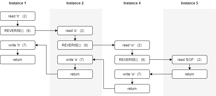
The arrows in the figure represent the order of execution of the statements in the computer. Each time we execute the recursive call to REVERSE in line 6, we create a new instance of the function, which starts its execution back at the beginning of the function (line 2). Then, when the function executes return, control reverts back to the next statement to be executed (line 7) in the calling instance of the function.
It’s important to understand that each instance of the function has its own set of variables whose values are unique to that instance. When we read n into the CHARACTER variable in the first instance of REVERSE it is not affected by anything that happens in the second instance of REVERSE. Therefore, reading the o into CHARACTER in the second instance of REVERSE does not affect the value of CHARACTER in the first instance of REVERSE.
During the execution of the first instance of REVERSE, the user enters the character n so the if condition is false and we execute the else part of the statement, which calls the REVERSE function. (Note that before we actually start the second instance of REVERSE, the operating system stores the statement where we will pick up execution once the called function returns.) When the second instance of REVERSE is started, a new copy of all variables is created as well to ensure we do not overwrite the values from the first instance.
The execution of the second instance of REVERSE runs exactly like the first instance except that the user enters the character o instead of n. Again, the else part of the if statement is executed, which calls the REVERSE function. When the third instance of REVERSE is executed, the user now inputs w, which again causes a new instance of REVERSE to be called.
Finally, in the fourth instance of REVERSE, the user inputs the * character, which causes the if part of the statement to execute, which performs our return statement. Once the return from the base case of our recursive function is performed, it starts the process of ending all the instances of the REVERSE function and creating the solution. When instance 4 of the REVERSE function returns, execution starts at the write statement (line 7) of instance 3. Here the character w is printed, and the function returns to instance 2. The same process is carried out in instance 2, which prints the o character and returns. Likewise, instance 1 prints its character n and then returns. The screen should now show the full output of the original call to REVERSE , which is “won”.
Recursion has allowed us to create a very simple and elegant solution to the problem of reversing an arbitrary number of characters. While you can do this in a non-recursive way using loops, the solution is not that simple. If you don’t believe us, just try it! (Yes, that is a challenge.)
 1function REVERSE2()
 2    read CHARACTER
 3    if CHARACTER == `*` then
 4        return
 5    else
 6        print CHARACTER
 7        REVERSE2()
 8        return
 9    end if
10end function
The REVERSE2 function in the previous quiz actually prints the characters entered by the user in the same order in which they are typed. Notice how this small variation in the instruction order significantly changed the outcome of the function. To get a better understanding of why this occurs, we will delve into the order of execution in a little more depth.
From the output of our original REVERSE function, we could argue that recursive function calls are carried out in a LIFO (last in, first out) order. Conversely, the output of the second version of the function REVERSE2, would lead us to believe that recursive function calls are carried out in FIFO (first in, first out) order. However, the ordering of the output is really based on how we structure our code within the recursive function itself, not the order of execution of the recursive functions.
To produce a LIFO ordering, we use a method called head recursion, which causes the function to make a recursive call first, then calculates the results once the recursive call returns. To produce a FIFO ordering, we use a method called tail recursion, which is when the function makes all of its necessary calculations before making a recursive call. With the REVERSE and REVERSE2 functions, this is simply a matter of swapping lines 6 and 7.
While some functions require the use of either head or tail recursion, many times we have the choice of which one to use. The choice is not necessarily just a matter of style, as we shall see next.
Before we finish our discussion of head and tail recursion, we need to make sure we understand how a recursive function actually works in the computer. To do this, we will use a new example. Let’s assume we want to print all numbers from 0 to $N$, where $N$ is provided as a parameter. A recursive solution to this problem is shown below.
 1function OUTPUT(integer N)
 2    if N == 0 then
 3        print N
 4    else
 5        print "Calling to OUTPUT " N-1
 6        OUTPUT(N-1)
 7        print "Returning from OUTPUT " N-1
 8        print N
 9    end if
10    return
11end function
Notice that we have added some extra print statements (lines 5 and 7) to the function just to help us keep track of when we have called OUTPUT and when that call has returned. This function is very similar to the REVERSE function above, we just don’t have to worry about reading a character each time the function runs. Now, if we call OUTPUT with an initial parameter of 3, we get the following output. We’ve also marked these lines with letters to make the following discussion simpler.
Calling to OUTPUT 2         (a)
Calling to OUTPUT 1         (b)
Calling to OUTPUT 0         (c)
0                           (d)
Returning from OUTPUT 0     (e)
1                           (f)
Returning from OUTPUT 1     (g)
2                           (h)
Returning from OUTPUT 2     (i)
3                           (j)
Lines a, b, and c show how the function makes all the recursive calls before any output or computation is performed. Thus, this is an example of head recursion which produces a LIFO ordering.
Once we get to the call of OUTPUT(0), the function prints out 0 (line d) and we start the return process. When we return from the call to OUTPUT(0) we immediately print out N, which is 1 and return. We continue this return process from lines g through j and eventually return from the original call to OUTPUT having completed the task.
Now that we have seen how recursion works in practice, we will pull back the covers and take a quick look at what is going on underneath. To be able to call the same function over and over, we need to be able to store the appropriate data related to each function call to ensure we can treat it as a unique instance of the function. While we do not make copies of the code, we do need to make copies of other data. Specifically, when function A calls function B, we must save the following information:
A to be executed when B returns (called the return address),B.We call this information the activation record for function A. When a call to B is made, this information is stored in a stack data structure known as the activation stack, and execution begins at the first instruction in function B. Upon completion of function B, the following steps are performed.
Next, we will look at how we use the activation stack to implement recursion. For this we will use a simple MAIN program that calls our simplified OUTPUT function (where we have removed all the print statements used to track our progress).
 1function MAIN()
 2    OUTPUT(3)
 3    print ("Done")
 4end function
 5
 6function OUTPUT(integer N)
 7    if N == 0 then
 8        print N
 9    else
10        OUTPUT(N-1)
11        print N
12    end if
13    return
14end function
When we run MAIN, the only record on the activation stack is the record for MAIN. Since it has not been “called” from another function, it does not contain a return address. It also has no local variables, so the record is basically empty as shown below.
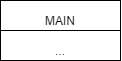
However, when we execute line 2 in MAIN, we call the function OUTPUT with a parameter of 3. This causes the creation of a new function activation record with the return address of line 3 in the calling MAIN function and a parameter for N, which is 3. Again, there are no local variables in OUTPUT. The stack activation is shown in figure a below.
| a | b | c | d |
|---|---|---|---|
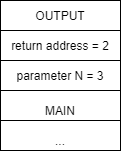
|
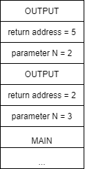
|
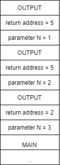
|
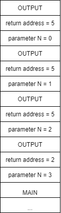
|
Following the execution for OUTPUT, we will eventually make our recursive call to OUTPUT in line 10, which creates a new activation record on the stack as shown above in b. This time, the return address will be line 11 and the parameter N is 2.
Execution of the second instance of OUTPUT will follow the first instance, eventually resulting in another recursive call to OUTPUT and a new activation record as shown in c above. Here the return address is again 5 but now the value of parameter N is 1. Execution of the third instance of OUTPUT yields similar results, giving us another activation record on the stack d with the value of parameter N being 0.
Finally, the execution of the fourth instance of OUTPUT will reach our base case of N == 0. Here we will write 0 in line 8 and then return. This return will cause us to start execution back in the third instance of OUTPUT at the line indicated by the return value, or in this case, 11. The stack activation will now look like e in the figure below.
| e | f | g | h |
|---|---|---|---|
|
|
|
|
|
When execution begins in the third instance of OUTPUT at line 11, we again write the current value of N, which is 1, and we then return. We follow this same process, returning to the second instance of OUTPUT, then the first instance of OUTPUT. Once the initial instance of OUTPUT completes, it returns to line 3 in MAIN, where the print("Done") statement is executed and MAIN ends.
While recursion is a very powerful technique, its expressive power has an associated cost in terms of both time and space. Anytime we call a function, a certain amount of memory space is needed to store information on the activation stack. In addition, the process of calling a function takes extra time since we must store parameter values and the return address, etc. before restarting execution. In the general case, a recursive function will take more time and more memory than a similar function computed using loops.
It is possible to demonstrate that any function with a recursive structure can be transformed into an iterative function that uses loops and vice versa. It is also important to know how to use both mechanisms because there are advantages and disadvantages for both iterative and recursive solutions. While we’ve discussed the fact that loops are typically faster and take less memory than similar recursive solutions, it is also true that recursive solutions are generally more elegant and easier to understand. Recursive functions can also allow us to find solutions to problems that are complex to write using loops.
The most popular example of using recursion is calculating the factorial of a positive integer $N$. The factorial of a positive integer $N$ is just the product of all the integers from $1$ to $N$. For example, the factorial of $5$, written as $5!$, is calculated as $5 * 4 * 3 * 2 * 1 = 120$. The definition of the factorial function itself is recursive.
$$ \text{fact}(N) = N * \text{fact}(N - 1) $$The corresponding pseudocode is shown below.
function FACT(N)
    if N == 1
        return 1
    else
        return N * FACT(N-1)
    end if
end function
The recursive version of the factorial is slower than the iterative version, especially for high values of $N$. However, the recursive version is simpler to program and more elegant, which typically results in programs that are easier to maintain over their lifetimes.
In the previous examples we saw recursive functions that call themselves one time within the code. This type of recursion is called linear recursion, where head and tail recursion are two specific types of linear recursion.
In this section we will investigate another type of recursion called tree recursion, which occurs when a function calls itself two or more times to solve a single problem. To illustrate tree recursion, we will use a simple recursive function MAX, which finds the maximum of $N$ elements in an array. To calculate the maximum of $N$ elements we will use the following recursive algorithm.
MAX1.MAX2.MAX1 and MAX2 to find the maximum of all elements.Our process recursively decomposes the problem by searching for the maximum in the first $N/2$ elements and the second $N/2$ elements until we reach the base case. In this problem, the base case is when we either have 1 or 2 elements in the array. If we just have 1, we return that value. If we have 2, we return the larger of those two values. An overview of the process is shown below.
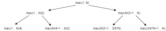
The pseudocode for the algorithm is shown below.
function MAX(VALUES, START, END)
    print "Called MAX with start = " + START + ", end = " + END
    if END – START = 0
        return VALUES[START]
    else if END – START = 1
        if VALUES(START) > VALUES(END)
            return VALUES[START]
        else
            return VALUES[END]
        end if
    else
        MIDDLE = ROUND((END – START) / 2)
        MAX1 = MAX(VALUES, START, START + MIDDLE – 1)
        MAX2 = MAX(VALUES, START + MIDDLE, END)
        if MAX1 > MAX2
            return MAX1
        else
            return MAX2
        end if
    end if
end function
The following block shows the output from the print line in the MAX function above. The initial call to the function is MAX(VALUES, 0, 15).
Called MAX with start = 0, end = 7
Called MAX with start = 0, end = 3
Called MAX with start = 0, end = 1
Called MAX with start = 2, end = 3
Called MAX with start = 4, end = 7
Called MAX with start = 4, end = 5
Called MAX with start = 6, end = 7
Called MAX with start = 8, end = 15
Called MAX with start = 8, end = 11
Called MAX with start = 8, end = 9
Called MAX with start = 10, end = 11
Called MAX with start = 12, end = 15
Called MAX with start = 12, end = 13
Called MAX with start = 14, end = 15
As you can see, MAX decomposes the array each time it is called, resulting in 14 instances of the MAX function being called. If we had performed head or tail recursion to compare each value in the array, we would have to have called MAX 16 times. While this may not seem like a huge savings, as the value of $N$ grows, so do the savings.
Next, we will look at calculating Fibonacci numbers using a tree recursive algorithm. Fibonacci numbers are given by the following recursive formula.
$$ f_n = f_{n-1} + f_{n-2} $$Notice that Fibonacci numbers are defined recursively, so they should be a perfect application of tree recursion! However, there are cases where recursive functions are too inefficient compared to an iterative version to be of practical use. This typically happens when the recursive solutions to a problem end up solving the same subproblems multiple times. Fibonacci numbers are a great example of this phenomenon.
To complete the definition, we need to specify the base case, which includes two values for the first two Fibonacci numbers: FIB(0) = 0 and FIB(1) = 1. The first Fibonacci numbers are $0, 1, 1, 2, 3, 5, 8, 13, 21 …$.
Producing the code for finding Fibonacci numbers is very easy from its definition. The extremely simple and elegant solution to computing Fibonacci numbers recursively is shown below.
function FIB(N)
    if N == 0
        return 0
    else if N == 1
        return 1
    else
        return FIB(N-1) + FIB(N-2)
    end if
end function
The following pseudocode performs the same calculations for the iterative version.
function FIBIT(N)
    FIB1 = 1
    FIB2 = 0
    for (I = 2 to N)
        FIB = FIB1 + FIB2
        FIB2 = FIB1
        FIB1 = FIB
    end loop
end function
While this function is not terribly difficult to understand, there is still quite a bit of mental gymnastics required to see how this implements the computation of Fibonacci numbers and even more to prove that it does so correctly. However, as we will see later, the performance improvements of the iterative solution are worth it.
If we analyze the computation required for the 6th Fibonacci number in both the iterative and recursive algorithms, the truth becomes evident. The recursive algorithm calculates the 5th Fibonacci number by recursively calling FIB(4) and FIB(3). In turn, FIB(4) calls FIB(3) and FIB(2). Notice that FIB(3) is actually calculated twice! This is a problem. If we calculate the 36th Fibonacci number, the values of many Fibonacci numbers are calculated repeatedly, over and over.
To clarify our ideas further, we can consider the recursive tree resulting from the trace of the program to calculate the 6th Fibonacci number. Each of the computations highlighted in the diagram will have been computed previously.
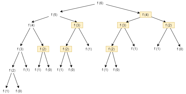
If we count the recomputations, we can see how we calculate the 4th Fibonacci number twice, the 3rd Fibonacci number three times, and the 2nd Fibonacci five times. All of this is due to the fact the we do not consider the work done by other recursive calls. Furthermore, the higher our initial number, the worse the situation grows, and at a very rapid pace.
To avoid recomputing the same Fibonacci number multiple times, we can save the results of various calculations and reuse them directly instead of recomputing them. This technique is called memoization, which can be used to optimize some functions that use tree recursion.
To implement memoization, we simply store the values the first time we compute them in an array. The following pseudocode shows an efficient algorithm that uses an array, called FA, to store and reuse Fibonacci numbers.
function FIBOPT(N)
    if N == 0
        return 0
    else if N == 1
        return 1
    else if FA[N] == -1
        FA[N] = FIBOPT(N-1) + FIBOPT(N-2)
        return FA[N]
    else
        return FA[N]
    end if
end function
We assume that each element in FA has been initialized to -1. We also assume that N is greater than 0 and that the length of FA is larger than the Fibonacci number N that we are trying to compute. (Of course, we would normally put these assumptions in our precondition; however, since we are focusing on the recursive nature of the function, we will not explicitly show this for now.) The cases where N == 0 and N == 1 are the same as we saw in our previous FIB function. There is no need to store these values in the array when we can return them directly, since storing them in the array takes additional time. The interesting cases are the last two. First, we check to see if FA[N] == -1, which would indicate that we have not computed the Fibonacci number for N yet. If we have not yet computed N’s Fibonacci number, we recursively call FIBOPT(N-1) and FIBOPT(N-2) to compute its value and then store it in the array and return it. If, however, we have already computed the Fibonacci for N (i.e., if FA[N] is not equal to -1), then we simply return the value stored in the array, FA[N].
As shown in our original call tree below, using the FIBOPT function, none of the function calls in red will be made at all. While the function calls in yellow will be made, they will simply return a precomputed value from the FA array. Notice that for N = 6, we save 14 of the original 25 function calls required for the FIB function, or a $56\%$ savings. As N increases, the savings grow even more.
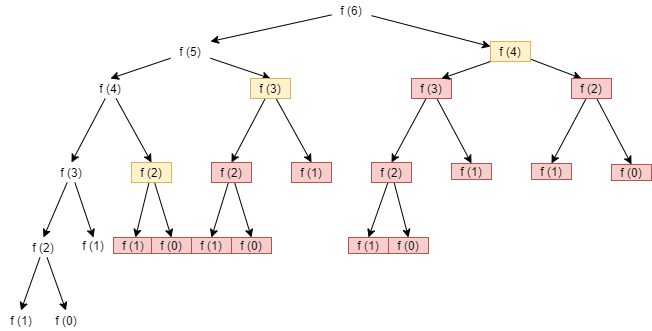
Memoization in Python can also be done using dictionaries or the functools.cache method decorator.
There are some problems where an iterative solution is difficult to implement and is not always immediately intuitive, while a recursive solution is simple, concise and easy to understand. A classic example is the problem of the Tower of Hanoi.
The Tower of Hanoi is a game that lends itself to a recursive solution. Suppose we have three towers on which we can put discs. The three towers are indicated by a letter, A, B, or C.
Now, suppose we have $N$ discs all of different sizes. The discs are stacked on tower A based on their size, smaller discs on top. The problem is to move all the discs from one tower to another by observing the following rules:
To try to solve the problem let’s start by considering a simple case: we want to move two discs from tower A to tower C. As a convenience, suppose we number the discs in ascending order by assigning the number 1 to the larger disc. The solution in this case is simple and consists of the following steps:
The following figure shows how the algorithm works.
It is a little more difficult with three discs, but after a few tries the proper algorithm emerges. With our knowledge of recursion, we can come up with a simple and concise solution. Since we already know how to move two discs from one place to another, we can solve the problem recursively.
In formulating our solution, we assumed that we could move two discs from one tower to another, since we have already solved that part of the problem above. In step 1, we use this solution to move the top two discs from tower A to B. Then, in step 3, we again use that solution to move two discs from tower B to C. This process can now easily be generalized to the case of N discs as described below.
The algorithm is captured in the following pseudocode. Here N is the total number of discs, ORIGIN is the tower where the discs are currently located, and DESTINATION is the tower where they need to be moved. Finally, TEMP is a temporary tower we can use to help with the move. All the parameters are integers.
function HANOI(N, ORIGIN, DESTINATION, TEMP)
    if N >= 0
        HANOI(N-1, ORIGIN, TEMP, DESTINATION)
        Move disc N from ORIGIN to DESTINATION
        HANOI(N-1, TEMP, DESTINATION, ORIGIN)
    end if
    return
end function
The function moves the $N$ discs from the source tower to the destination tower using a temporary tower. To do this, it calls itself to move the first $N-1$ discs from the source tower to the temporary tower. It then moves the bottom disc from the source tower to the destination tower. The function then moves the $N-1$ discs present in the temporary tower into the destination tower.
The list of movements to solve the three-disc problem is shown below.
Iterative solutions to the Tower of Hanoi problem do exist, but it took many researchers several years to find an efficient solution. The simplicity of finding the recursive solution presented here should convince you that recursion is an approach you should definitely keep in your bag of tricks!
Iteration and recursion have the same expressive power, which means that any problem that has a recursive solution also has an iterative solution and vice versa. There are also standard techniques that allow you to transform a recursive program into an equivalent iterative version. The simplest case is for tail recursion, where the recursive call is the last step in the function. There are two cases of tail recursion to consider when converting to an iterative version.
f(x) executes is a call to itself, f(y) with parameter y, the recursive call can be replaced by an assignment statement, x = y, and by looping back to the beginning of function f.The approach above only solves the conversion problem in the case of tail recursion. However, as an example, consider our original FACT function and its iterative version FACT2. Notice that in FACT2 we had to add a variable fact to keep track of the actual computation.
function FACT(N)
    if N == 1
        return 1
    else
        return N * FACT(N-1)
    end if
end function
function FACT2(N)
fact = 1
while N > 0
fact = fact * N
N = N - 1
end while
return fact
end functionThe conversion of non-tail recursive functions typically uses two loops to iterate through the process, effectively replacing recursive calls. The first loop executes statements before the original recursive call, while the second loop executes the statements after the original recursive call. The process also requires that we use a stack to save the parameter and local variable values each time through the loop. Within the first loop, all the statements that precede the recursive call are executed, and then, before the loop terminates, the values of interest are pushed onto the stack. The second loop starts by popping the values saved on the stack and then executing the remaining statements that come after the original recursive call. This is typically much more difficult than the conversion process for tail recursion.
In this module, we explored the use of recursion to write concise solutions for a variety of problems. Recursion allows us to call a function from within itself, using either head recursion, tail recursion or tree recursion to solve smaller instances of the original problem.
Recursion requires a base case, which tells our function when to stop calling itself and start returning values, and a recursive case to handle reducing the problem’s size and calling the function again, sometimes multiple times.
We can use recursion in many different ways, and any problem that can be solved iteratively can also be solved recursively. The power in recursion comes from its simplicity in code—some problems are much easier to solve recursively than iteratively.
Unfortunately, in general a recursive solution requires more computation time and memory than an iterative solution. We can use techniques such as memoization to greatly improve the time it takes for a recursive function to execute, especially in the case of calculating Fibonacci numbers where subproblems are overlapped.
Methods for finding and organizing data!
In this course, we are learning about many different ways we can store data in our programs, using arrays, queues, stacks, lists, maps, and more. We’ve already covered a few of these data structures, and we’ll learn about the others in upcoming modules. Before we get there, we should also look at a couple of the most important operations we can perform on those data structures.
Consider the classic example of a data structure containing information about students in a school. In the simplest case, we could use an array to store objects created from a Student class, each one representing a single student in the school.
As we’ve seen before, we can easily create those objects and store them in our array. We can even iterate through the array to find the maximum age or minimum GPA of all the students in our school. However, what if we want to just find a single student’s information? To do that, we’ll need to discuss one of the most commonly used data structure operations: searching.
Searching typically involves finding a piece of information, or a value stored in a data structure or calculated within a specific domain. For example, we might want to find out if a specific word is found in an array of character strings. We might also want to find an integer that meets a specific criterion, such as finding an integer that is the sum of the two preceding integers. For this module, we will focus on finding values in data structures.
In general, we can search for
The data structure can be thought of more generally as a container, which can be
For the examples in this module, we’ll generally use a simple finite array as our container. However, it shouldn’t be too difficult to figure out how to expand these examples to work with a larger variety of data structures. In fact, as we introduce more complex data structures in this course, we’ll keep revisiting the concept of searching and see how it applies to the new structure.
In general, containers can be either ordered or unordered. In many cases, we may also use the term sorted to refer to an ordered container, but technically an ordered container just enforces an ordering on values, but they may not be in a sorted order. As long as we understand what the ordering is, we can use that to our advantage, as we’ll see later.
Searches in an unordered container generally require a linear search, where every value in the container must be compared against our search value. On the other hand, search algorithms on ordered containers can take advantage of this ordering to make their searches more efficient. A good example of this is binary search. Let’s begin by looking at the simplest case, linear search.
When searching for a number in an unordered array, our search algorithms are typically designed as functions that take two parameters:
Our search functions then return an index to the number within the array.
In this module, we will develop a couple of examples of searching an array for a specific number.
Finding the first occurrence of a number in an unordered array is a fairly straightforward process. A black box depiction of this function is shown below. There are two inputs, array and number, and a single output, the index of the first occurrence of the number in array.
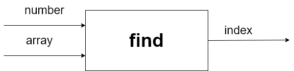
We can also include the search function as a method inside of the container itself. In that case, we don’t have to accept the container as a parameter, since the method will know to refer to the object it is part of.
Of course, when we begin designing an algorithm for our function we should think about two items immediately: the preconditions and the postconditions of the function. For this function, they are fairly simple.
The precondition for find is that the number provided as input is compatible with the type of data held by the provided array. In this case, we have no real stipulations on array. It does not need to actually have any data in it, nor does it have to be ordered or unordered.
Our postcondition is also straightforward. The function should return the index of number if it exists in the array. However, if number is not found in the array, then -1 is returned. Depending on how we wish to implement this function, it could also return another default index or throw an exception if the desired value is not found. However, most searching algorithms follow the convention of returning an invalid index of -1 when the value is not found in the array, so that’s what we’ll use in our examples.
Preconditions:
Postconditions:
To search for a single number in our array, we will use a loop to search each location in the array until we find the number. The general idea is to iterate over all the elements in the array until we either find the number we are searching for or there are no other elements in the array.
1function FIND(NUMBER, ARRAY)
2    loop INDEX from 0 to size of ARRAY - 1
3        if ARRAY[INDEX] == NUMBER
4            return INDEX
5        end if
6    end for
7    return -1
8end function
As we can see in line 1, the function takes both a number and array parameter. We then enter a for loop in line 2 to loop through each location in the array. We keep track of the current location in the array using the index variable. For each location, we compare number against the value in the array at location index. If we find the number, we simply return the value of index in line 4. If we do not find the number anywhere in the array, the loop will exit, and the function will return -1 in line 8.
Below is an example of how to execute this algorithm on example data. Step 1 shows the initial state of the variables in the function the first time through the loop. Both array and number are passed to the function but we do not modify either of them in the function. The index variable is the for loop variable, which is initially set to 0 the first time through the loop. In line 3, the function compares the number in array[index] against the value of number. In this step, since index is 0, we use array[0], which is 8. Since 8 is not equal to the value of number, which is 3, we do nothing in the if statement and fall to the end for statement in line 6. Of course, this just sends us back to the for statement in line 2.
The second time through the for loop is shown as Step 2 in the figure. We follow the same logic as above and compare array[1], or 4, against number, which is still 3. Since these values are not equal, we skip the rest of the if statement and move on to Step 3.
In Step 3, index is incremented to 2, thus pointing at array[2], whose value is 3. Since this value is equal to the value of number, we carry out the if part of the statement. Line 4 returns the value of 2, which is the first location in array that holds the value of number.

Our find algorithm above will find the first instance of number in the array and return the index of that instance. However, we might also be interested in finding the last instance of number in array. Looking at our original find algorithm, it should be easy to find the last value by simply searching the array in reverse order, as shown in the following figure.
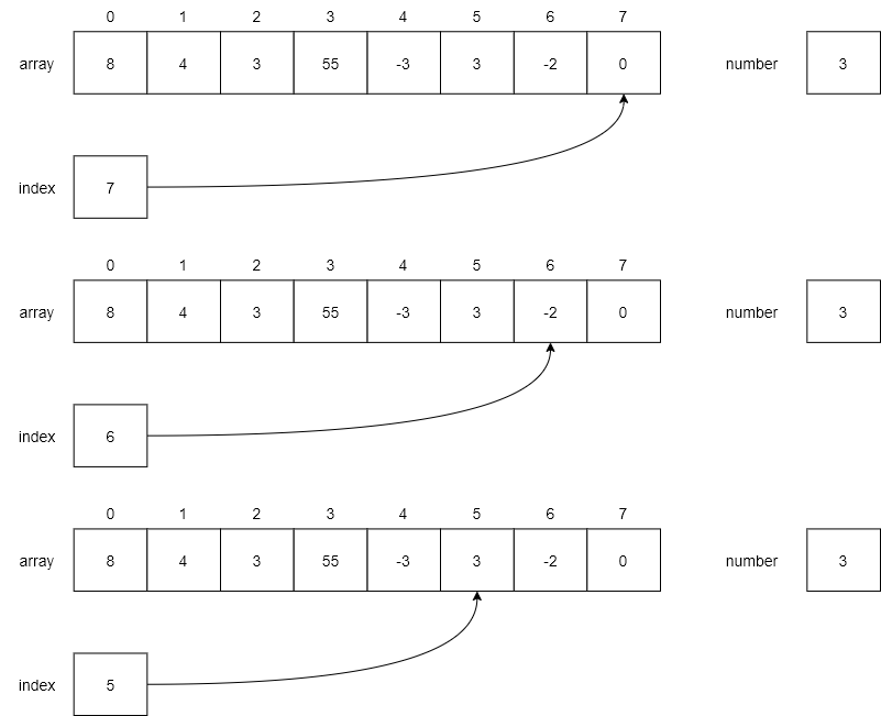
We will use the same example as above, except we will start searching backwards from the end of the array. In Step 1, we see that index is initialized to 7 and we compare array[7] against number, which are not the same. Thus, we continue to Step 2, where we decrement index to 6. Here array[6] is still not equal to number, so we continue in the loop. Finally, in Step 3, we decrement index to 5. Now array[5] contains the number 3, which is equal to our number and we return the current index value.
Luckily for us, we can change our for loop index to decrement from the end of the array (size of array - 1) to the beginning (0). Thus, by simply changing line 3 in our original function, we can create a new function that searches for the last instance of number in array. The new function is shown below.
1function REVERSEFIND(NUMBER, ARRAY)
2    loop INDEX from size of ARRAY – 1 to 0 step -1
3        if ARRAY[INDEX] == NUMBER
4            return INDEX
5        end if
6    end for
7    return -1
8end function
Obviously, the for loop in line 2 holds the key to searching our array in reverse order. We start at the end of the array by using the index size of array - 1 and then decrement the value of index (via the step -1 qualifier) each time through the loop until we reach 0. The remainder of the function works exactly like the find function.
We looked at an iterative version of the find function above. But what would it take to turn that function into a recursive function? While for this particular function, there is not a lot to be gained from the recursive version, it is still instructive to see how we would do it. We will find recursive functions more useful later on in the module.
In this case, to implement a recursive version of the function, we need to add a third parameter, index, to tell us where to check in the array. We assume that at the beginning of a search, index begins at 0. Then, if number is not in location index in the array, index will be incremented before making another recursive call. Of course, if number is in location index, we will return the number of index. The pseudocode for the findR function is shown below.
1function FINDR (NUMBER, ARRAY, INDEX)
2    if INDEX >= size of ARRAY then
3        return -1
4    else if ARRAY[INDEX] == NUMBER
5        return INDEX
6    else
7        return FINDR (NUMBER, ARRAY, INDEX + 1)
8    end if
9end function
First, we check to see if index has moved beyond the bounds of the array, which would indicate that we have searched all the locations in array for number. If that is the case, then we return -1 in line 3 indicating that we did not find number in array. Next, we check to see if number is found in array[index] in line 4. If it is, the we are successful and return the index. However, if we are not finished searching and we have not found number, then we recursively call findR and increment index by 1 to search the next location.
An example of using the findR function is shown below. The top half of the figure shows the state of the data in the initial call to the findR function (instance 1). The bottom half of the figure shows the recursive path through the function. The beginning of instance 1 shows the if statement in line 2. In instance 1, since we have not searched the entire array (line 2) and array[0] is not equal to number (line 4), we fall down to the else part function and execute line 7, the recursive call. Since index is 0 in instance 1, we call instance 2 of the function with an index of 1.
In instance 2, the same thing happens as in instance 1 and we fall down to the else part of the if statement. Once again, we call a new instance of findR, this time with index set at 2. Now, in instance 3, array[index] is equal to number in line 4 and so we execute the return index statement in line 5. The value of index (2) is returned to instance 2, which, in line 7, simply returns the value of 2 to instance 1. Again, in line 7, instance 1 returns that same value (2) to the original calling function.
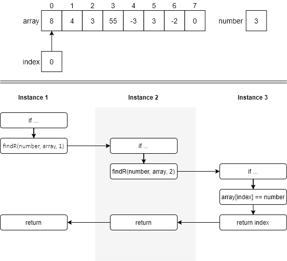
Notice that the actual process of searching the array is the same for both the iterative and recursive functions. It is only the implementation of that process that is different between the two.
We may also want to search through a data structure to find an item with a specific property. For example, we could search for the student with the maximum age, or the minimum GPA. For this example, let’s consider the case where we’d like to find the minimum value in an array of integers.
Searching for the minimum number in an unordered array is a different problem than searching for a specific number. First of all, we do not know what number we are searching for. And, since the array is not ordered, we will have to check each and every number in the array.
The input parameters of our new function will be different from the find function above, since we do not have a number to search for. In this case, we only have an array of numbers as an input parameter. The output parameter, however, is the same. We still want to return the index of the minimum number in the array. In this case, we will return -1 if there is no minimum number, which can only happen if there is no data in the array when we begin.
Preconditions:
Postconditions:
Our preconditions and postconditions are also simple. Our precondition is simply that we have an array whose data can be sorted. This is important, because it means that we can compare two elements in the array and determine which one has a smaller value. Otherwise, we couldn’t determine the minimum value at all!
Our postcondition is that we return the minimum number of the data in the array, or -1 if the array is empty.
The function findMin is shown below. First, we check to see if the array is empty. If it is, we simply return -1 in line 3. If not, we assume the location 0 contains the minimum number in the array, and set min equal to 0 in line 5. Then we loop through each location in the array (starting with 1) in line 6 and set min equal to the minimum of the array data at the current index and the data at min. (Note: if the array only has a single number in it, the for loop will not actually execute since index will be initialized to 1, which is already larger than the size of the array – 1, which is 0.) Once we complete the loop, we will be guaranteed that we have the index of the minimum number in the array.
 1function FINDMIN(ARRAY)
 2    if ARRAY is empty then
 3        return -1
 4    end if
 5    MIN = 0
 6    loop INDEX from 1 to size of ARRAY - 1
 7        if ARRAY[INDEX] < ARRAY[MIN]
 8            MIN = INDEX
 9        end if
10    end for
11    return MIN
12end function
Next, we will walk through the algorithm using our example array in the figure below. Step 1 shows the initial time through the loop. In line 5, min is set to 0 by default and in line 6, index is set equal to 1. Line 7 then computes whether array[1] < array[0]. In this case, it is and we set min = 1 (which is reflected in the next step where min has the value 1).
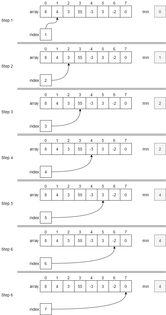
Step 2 will end up comparing array[2] < array[1], since min is now 1 and index has been incremented to 2 via the for loop. In this case, array[2] is less than array[1] so we update min again, this time to 2.
Step 3 follows the same process; however, this time the value in array[3] is 55, which is greater than the current minimum of 3 in array[2]. Therefore, min is not updated. Step 4 finds the minimum value in the array of -3 at index 4 and so updates min to 4. However, steps 5, 6, and 7 do not find new minimum values. Thus, when the loop exits after Step 6, min is set to 4 and this value is returned to the calling program in line 11.
We’ve examined many different versions of a linear search algorithm. We can find the first occurrence of a number in an array, the last occurrence of that number, or a value with a particular property, such as the minimum value. Each of these are examples of a linear search, since we look at each element in the container sequentially until we find what we are looking for.
So, what would be the time complexity of this process? To understand that, we must consider what the worst-case input would be. For this discussion, we’ll just look at the find function, but the results are similar for many other forms of linear search. The pseudocode for find is included below for reference.
1function FIND(NUMBER, ARRAY)
2    loop INDEX from 0 to size of ARRAY - 1
3        if ARRAY[INDEX] == NUMBER
4            return INDEX
5        end if
6    end for
7    return -1
8end function
How would we determine what the worst-case input for this function would be? In this case, we want to come up with the input that would require the most steps to find the answer, regardless of the size of the container. Obviously, it would take more steps to find a value in a larger container, but that doesn’t really tell us what the worst-case input would be.
Therefore, the time complexity for a linear search algorithm is clearly proportional to the number of items that we need to search through, in this case the size of our array. Whether we use an iterative algorithm or a recursive algorithm, we still need to search the array one item at a time. We’ll refer to the size of the array as $N$.
Here’s the key: when searching for minimum or maximum values, the search will always take exactly $N$ comparisons since we have to check each value. However, if we are searching for a specific value, the actual number of comparisons required may be fewer than $N$.
To build a worst-case input for the find function, we would search for the situation where the value to find is either the last value in the array, or it is not present at all. For example, consider the array we’ve been using to explore each linear search algorithm so far.
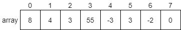
What if we are trying to find the value 55 in this array? In that case, we’ll end up looking at 4 of the 8 elements in the array. This would take $N/2$ steps. Can we think of another input that would be worse?
Consider the case where we try to find 0 instead. Will that be worse? In that case, we’ll need to look at all 8 elements in the array before we find it. That requires $N$ steps!
What if we are asked to find 1 in the array? Since 1 is not in the array, we’ll have to look at every single element before we know that it can’t be found. Once again, that requires $N$ steps.
We could say that in the worst-case, a linear search algorithm requires “on the order of $N$” time to find an answer. Put another way, if we double the size of the array, we would also need to double the expected number of steps required to find an item in the worst case. We sometimes call this linear time, since the number of steps required grows at the same rate as the size of the input.
Our question now becomes, “Is a search that takes on the order of $N$ time really all that bad?”. Actually, it depends. Obviously, if $N$ is a small number (less than 1000 or so) it may not be a big deal, if you only do a single search. However, what if we need to do many searches? Is there something we can do to make the process of searching for elements even easier?
Let’s consider the real world once again for some insights. For example, think of a pile of loose papers on the floor. If we wanted to find a specific paper, how would we do it?
In most cases, we would simply have to perform a linear search, picking up each paper one at a time and seeing if it is the one we need. This is pretty inefficient, especially if the pile of papers is large.
What if we stored the papers in a filing cabinet and organized them somehow? For example, could we sort the papers by title in alphabetical order? Then, when we want to find a particular paper, we can just skip to the section that contains files with the desired first letter and go from there. In fact, we could even do this for the second and third letter, continuing to jump forward in the filing cabinet until we found the paper we need.
This seems like a much more efficient way to go about searching for things. In fact, we do this naturally without even realizing it. Most computers have a way to sort files alphabetically when viewing the file system, and anyone who has a collection of items has probably spent time organizing and alphabetizing the collection to make it easier to find specific items.
Therefore, if we can come up with a way to organize the elements in our array, we may be able to make the process of finding a particular item much more efficient. In the next section, we’ll look at how we can use various sorting algorithms to do just that.
File:FileStack retouched.jpg. (2019, January 17). Wikimedia Commons, the free media repository. Retrieved 22:12, March 23, 2020 from https://commons.wikimedia.org/w/index.php?title=File:FileStack_retouched.jpg&oldid=335159723. ↩︎
File:Istituto agronomico per l’oltremare, int., biblioteca, schedario 05.JPG. (2016, May 1). Wikimedia Commons, the free media repository. Retrieved 22:11, March 23, 2020 from https://commons.wikimedia.org/w/index.php?title=File:Istituto_agronomico_per_l%27oltremare,_int.,_biblioteca,_schedario_05.JPG&oldid=194959053. ↩︎
Sorting is the process we use to organize an ordered container in a way that we understand what the ordering of the values represents. Recall that an ordered container just enforces an ordering between values, but that ordering may appear to be random. By sorting an ordered container, we can enforce a specific ordering on the elements in the container, allowing us to more quickly find specific elements as we’ll see later in this chapter.
In most cases, we sort values in either ascending or descending order. Ascending order means that the smallest value will be first, and then each value will get progressively larger until the largest value, which is at the end of the container. Descending order is the opposite—the largest value will be first, and then values will get progressively smaller until the smallest value is last.
We can also define this mathematically. Assume that we have a container called array and two indexes in that container, a and b. If the container is sorted in ascending order, we would say that if a is less than b (that is, the element at index a comes before the element at index b), then the element at index a is less than or equal to the element at index b. More succinctly:
Likewise, if the container is sorted in descending order, we would know that if a is less than b, then the element at index a would be greater than or equal to the element at index b. Or:
These facts will be important later when we discuss the precondition, postconditions, and loop invariants of algorithms in this section.
To sort a collection of data, we can use one of many sorting algorithms to perform that action. While there are many different algorithms out there for sorting, there are a few commonly used algorithms for this process, each one with its own pros, cons, and time complexity. These algorithms are studied extensively by programmers, and nearly every programmer learns how to write and use these algorithms as part of their learning process. In this module, we’ll introduce you to the 4 most commonly used sorting algorithms:
The first sorting algorithm we’ll learn about is selection sort. The basic idea behind selection sort is to search for the minimum value in the whole container, and place it in the first index. Then, repeat the process for the second smallest value and the second index, and so on until the container is sorted.
Wikipedia includes a great animation that shows this process:
In this animation, the element highlighted in blue is the element currently being considered. The red element shows the value that is the minimum value considered, and the yellow elements are the sorted portion of the list.
Let’s look at a few steps in this process to see how it works. First, the algorithm will search through the array to find the minimum value. It will start by looking at index 0 as shown in the figure below.
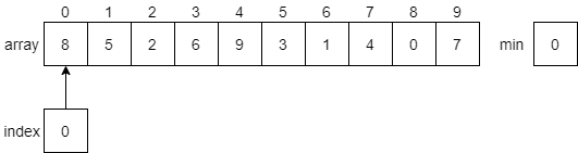
Once it reaches the end of the array, it will find that the smallest value 0 is at index 8.
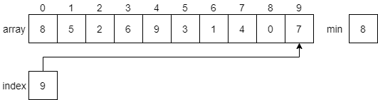
Then, it will swap the minimum item with the item at index 0 of the array, placing the smallest item first. That item will now be part of the sorted array, so we’ll shade it in since we don’t want to move it again.
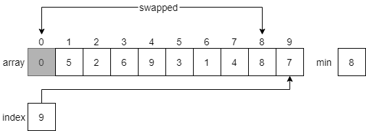
Next, it will reset index to 1, and start searching for the next smallest element in the array. Notice that this time it will not look at the element at index 0, which is part of the sorted array. Each time the algorithm resets, it will start looking at the element directly after the sorted portion of the array.
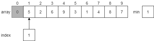
Once again, it will search through the array to find the smallest value, which will be the value 1 at index 6.
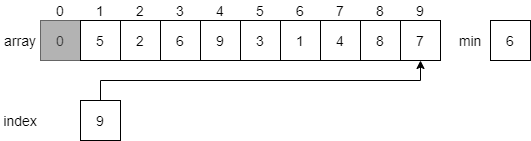
Then, it will swap the element at index 1 with the minimum element, this time at index 6. Just like before, we’ll shade in the first element since it is now part of the sorted list, and reset the index to begin at index 2
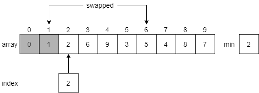
This process will repeat until the entire array is sorted in ascending order.
File:Selection-Sort-Animation.gif. (2016, February 12). Wikimedia Commons, the free media repository. Retrieved 22:22, March 23, 2020 from https://commons.wikimedia.org/w/index.php?title=File:Selection-Sort-Animation.gif&oldid=187411773. ↩︎
To describe our selection sort algorithm, we can start with these basic preconditions and postconditions.
Preconditions:
Postconditions:
We can then represent this algorithm using the following pseudocode.
 1function SELECTIONSORT(ARRAY)
 2    loop INDEX from 0 to size of ARRAY – 2
 3      MININDEX = 0
 4        # find minimum index
 5        loop INDEX2 from INDEX to size of ARRAY – 1
 6            if ARRAY[INDEX2] < ARRAY[MININDEX] then
 7                MININDEX = INDEX
 8            end if
 9        end loop
10        # swap elements
11        TEMP = ARRAY[MININDEX]
12        ARRAY[MININDEX] = ARRAY[INDEX]
13        ARRAY[INDEX] = TEMP
14    end loop
15end function
In this code, we begin by looping through every element in the array except the last one, as seen on line 2. We don’t include this one because if the rest of the array is sorted properly, then the last element must be the maximum value.
Lines 3 through 9 are basically the same as what we saw in our findMin function earlier. It will find the index of the minimum value starting at INDEX through the end of the array. Notice that we are starting at INDEX instead of the beginning. As the outer loop moves through the array, the inner loop will consider fewer and fewer elements. This is because the front of the array contains our sorted elements, and we don’t want to change them once they are in place.
Lines 11 through 13 will then swap the elements at INDEX and MININDEX, putting the smallest element left in the array at the position pointed to by index.
We can describe the invariant of our outer loop as follows:
index is sorted in ascending order.The second part of the loop invariant is very important. Without that distinction, we could simply place new values into the array before index and satisfy the first part of the invariant. It is always important to specify that the array itself still contains the same elements as before.
Let’s look at the time complexity of the selection sort algorithm, just so we can get a feel for how much time this operation takes.
First, we must determine if there is a worst-case input for selection sort. Can we think of any particular input which would require more steps to complete?
In this case, each iteration of selection sort will look at the same number of elements, no matter what they are. So there isn’t a particular input that would be considered worst-case. We can proceed with just the general case.
In each iteration of the algorithm we need to search for the minimum value of the remaining elements in the container. If the container has $N$ elements, we would follow the steps below.
This process continues until we have sorted all of the elements in the array. The number of steps will be:
$$ N + (N – 1) + (N – 2) + … + 2 + 1 $$While it takes a bit of math to figure out exactly what that means, we can use some intuition to determine an approximate value. For example we could pair up the values like this:
$$ N + [(N – 1) + 1] + [(N – 2) + 2] + ... $$When we do that, we’ll see that we can create around $N / 2$ pairs, each one with the value of $N$. So a rough approximation of this value is $N * (N / 2)$, which is $N^2 / 2$. When analyzing time complexity, we would say that this is “on the order of $N^2$” time. Put another way, if the size of $N$ doubles, we would expect the number of steps to go up by a factor of $4$, since $(2 * N)^2 = 4N$.
Later on, we’ll come back to this and compare the time complexity of each sorting algorithm and searching algorithm to see how they stack up against each other.
Next, let’s look at another sorting algorithm, bubble sort. The basic idea behind bubble sort is to continuously iterate through the array and swap adjacent elements that are out of order. As a side effect of this process, the largest element in the array will be “bubbled” to the end of the array after the first iteration. Subsequent iterations will do the same for each of the next largest elements, until eventually the entire list is sorted.
Wikipedia includes a great animation that shows this process:
In this animation, the two red boxes slowly move through the array, comparing adjacent elements. If the elements are not in the correct order (that is, the first element is larger than the second element), then it will swap them. Once it reaches the end, the largest element, 8, will be placed at the end and locked in place.
Let’s walk through a few steps of this process and see how it works. We’ll use the array we used previously for selection sort, just to keep things simple. At first, the array will look like the diagram below.
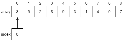
We’ll begin with the index variable pointing at index 0. Our algorithm should compare the values at index 0 and index 1 and see if they need to be swapped. We’ll put a bold border around the elements we are currently comparing in the figure below.
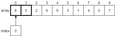
Since the element at index 0 is 8, and the element at index 1 is 5, we know that they must be swapped since 8 is greater than 5. We need to swap those two elements in the array, as shown below.
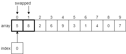
Once those two elements have been swapped, the index variable will be incremented by 1, and we’ll look at the elements at indexes 1 and 2 next.
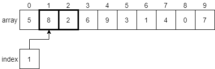
Since 8 is greater than 2, we’ll swap these two elements before incrementing index to 2 and comparing the next two elements.
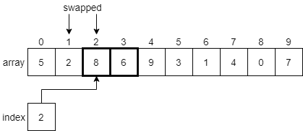
Again, we’ll find that 8 is greater than 6, so we’ll swap these two elements and move on to index 3.
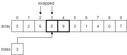
Now we are looking at the element at index 3, which is 8, and the element at index 4, which is 9. In this case, 8 is less than 9, so we don’t need to swap anything. We’ll just increment index by 1 and look at the elements at indexes 4 and 5.
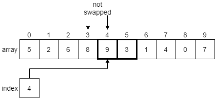
As we’ve done before, we’ll find that 9 is greater than 3, so we’ll need to swap those two items. In fact, as we continue to move through the array, we’ll find that 9 is the largest item in the entire array, so we’ll end up swapping it with every element down to the end of the array. At that point, it will be in its final position, so we’ll lock it and restart the process again.
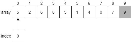
After making a second pass through the array, swapping elements that must be swapped as we find them, we’ll eventually get to the end and find that 8 should be placed at index 8 since it is the next largest value in the array.
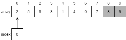
We can then continue this process until we have locked each element in place at the end of the array.
File:Bubble-sort-example-300px.gif. (2019, June 12). Wikimedia Commons, the free media repository. Retrieved 22:36, March 23, 2020 from https://commons.wikimedia.org/w/index.php?title=File:Bubble-sort-example-300px.gif&oldid=354097364. ↩︎
To describe our bubble algorithm, we can start with these basic preconditions and postconditions.
Preconditions:
Postconditions:
We can then represent this algorithm using the following pseudocode.
 1function BUBBLESORT(ARRAY)
 2    # loop through the array multiple times
 3    loop INDEX from 0 to size of ARRAY – 1
 4        # consider every pair of elements except the sorted ones
 5        loop INDEX2 from 0 to size of ARRAY – 2 – INDEX
 6            if ARRAY[INDEX2] > ARRAY[INDEX2 + 1] then
 7                # swap elements if they are out of order
 8                TEMP = ARRAY[INDEX2]
 9                ARRAY[INDEX2] = ARRAY[INDEX2 + 1]
10                ARRAY[INDEX2 + 1] = TEMP
11            end if
12        end loop
13    end loop
14end function
In this code, we begin by looping through every element in the array, as seen on line 3. Each time we run this outer loop, we’ll lock one additional element in place at the end of the array. Therefore, we need to run it once for each element in the array.
On line 5, we’ll start at the beginning of the array and loop to the place where the sorted portion of the array begins. We know that after each iteration of the outer loop, the value index will represent the number of locked elements at the end of the array. We can subtract that value from the end of the array to find where we want to stop.
Line 6 is a comparison between two adjacent elements in the array starting at the index index2. If they are out of order, we use lines 8 through 10 to swap them. That’s really all it takes to do a bubble sort!
Looking at this code, we can describe the invariant of our outer loop as follows:
index elements in the array are in sorted order, andNotice how this differs from selection sort, since it places the sorted elements at the beginning of the array instead of the end. However, the result is the same, and by the end of the program we can show that each algorithm has fully sorted the array.
Once again, let’s look at the time complexity of the bubble sort algorithm and see how it compares to selection sort.
Bubble sort is a bit trickier to analyze than selection sort, because there are really two parts to the algorithm:
Let’s look at each one individually. First, is there a way to reduce the number of comparisons made by this algorithm just by changing the input? As it turns out, there isn’t anything we can do to change that based on how it is written. The number of comparisons only depends on the size of the array. In fact, the analysis is exactly the same as selection sort, since each iteration of the outer loop does one fewer comparison. Therefore, we can say that bubble sort has time complexity on the order of $N^2$ time when it comes to comparisons.
What about swaps? This is where it gets a bit tricky. What would be the worst-case input for the bubble sort algorithm, which would result in the largest number of swaps made?
Consider a case where the input is sorted in descending order. The largest element will be first, and the smallest element will be last. If we want the result to be sorted in ascending order, we would end up making $N - 1$ swaps to get the first element to the end of the array, then $N - 2$ swaps for the second element, and so on. So, once again we end up with the same series as before:
$$ (N – 1) + (N – 2) + ... + 2 + 1. $$In the worst-case, we’ll also end up doing on the order of $N^2$ swaps, so bubble sort has a time complexity on the order of $N^2$ time when it comes to swaps as well.
It seems that both bubble sort and selection sort are in the same order of time complexity, meaning that each one will take roughly the same amount of time to sort the same array. Does that tell us anything about the process of sorting an array?
Here’s one way to think about it: what if we decided to compare each element in an array to every other element? How many comparisons would that take? We can use our intuition to know that each element in an array of $N$ elements would require $N – 1$ comparisons, so the total number of comparisons would be $N * (N – 1)$, which is very close to $N^2$.
Of course, once we’ve compared each element to every other element, we’d know exactly where to place them in a sorted array. One possible conclusion we could make is that there isn’t any way to sort an array that runs much faster than an algorithm that runs in the order of $N^2$ time.
Thankfully, that conclusion is incorrect! There are several other sorting algorithms we can use that allow us to sort an array much more quickly than $N^2$ time. Let’s take a look at those algorithms and see how they work!
Another commonly used sorting algorithm is merge sort. Merge sort uses a recursive, divide and conquer approach to sorting, which makes it very powerful. It was actually developed to handle sorting data sets that were so large that they couldn’t fit on a single memory device, way back in the early days of computing.
The basic idea of the merge sort algorithm is as follows:
Once again, Wikipedia has a great animation showing this process:
Let’s walk through a simple example and see how it works. First, we’ll start with the same initial array as before, shown in the figure below. To help us keep track, we’ll refer to this function call using the array indexes it covers. It will be mergeSort(0, 9).
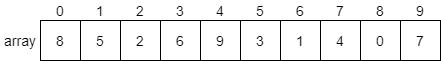
Since this array contains more than 2 elements, we won’t be able to sort it quickly. Instead, we’ll divide it in half, and sort each half using merge sort again. Let’s continue the process with the first half of the array. We’ll use a thick outline to show the current portion of the array we are sorting, but we’ll retain the original array indexes to help keep track of everything.

Now we are in the first recursive call, mergeSort(0, 4),which is looking at the first half of the original array. Once again, we have more than 2 elements, so we’ll split it in half and recursively call mergeSort(0, 1) first.

At this point, we now have an array with just 2 elements. We can use one of our base cases to sort that array by swapping the two elements, if needed. In this case, we should swap them, so we’ll get the result shown below.
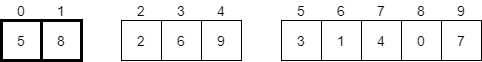
Now that the first half of the smaller array has been sorted, our recursive call mergeSort(0, 1) will return and we’ll look at the second half of the smaller array in the second recursive call, mergeSort(2, 4), as highlighted below.
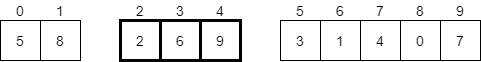
As we’ve seen before, this array has more than 2 elements, so we’ll need to divide it in half and recursively call the function again. First, we’ll call mergeSort(2, 2).
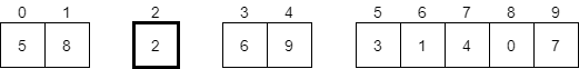
In this case, the current array we are considering contains a single element, so it is already sorted. Therefore, the recursive call to mergeSort(2, 2) will return quickly, and we’ll consider the second part of the smaller array in mergeSort(3, 4), highlighted below.
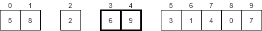
Here, we have 2 elements, and this time they are already sorted. So, we don’t need to do anything, and our recursive call to mergeSort(3, 4) will return. At this point, we will be back in our call to mergeSort(2, 4), and both halves of that array have been sorted. We’re back to looking at the highlighted elements below.
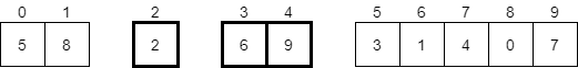
Now we have to merge these two arrays together. Thankfully, since they are sorted, we can follow this simple process:
Let’s take a look at what that process would look like. First, we’ll create a new temporary array to store the result.
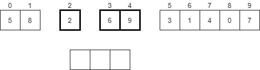
Next, we will look at the first element in each of the two sorted halves of the original array. In this case, we’ll compare 2 and 6, which are highlighted below.
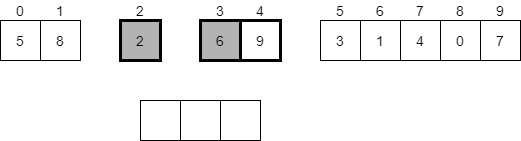
Now we should pick the smaller of those two values, which will be 2. That value will be placed in the new temporary array at the very beginning.

Next, we should look at the remaining halves of the array. Since the first half is empty, we can just place the remaining elements from the second half into the temporary array.
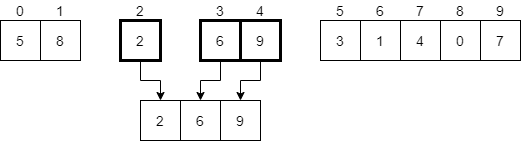
Finally, we should replace the portion of the original array that we are looking at in this recursive call with the temporary array. In most cases, we’ll just copy these elements into the correct places in the original array. In the diagram, we’ll just replace them.

There we go! We’ve now completed the recursive call mergeSort(2, 4). We can return from that recursive call and go back to mergeSort(0, 4).
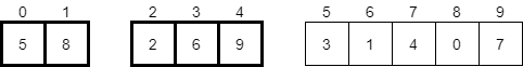
Since both halves of the array in mergeSort(0, 4) are sorted, we must do the merge process again. We’ll start with a new temporary array and compare the first element in each half.
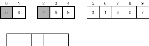
At this point, we’ll see that 2 is the smaller of those elements, so we’ll place it in the first slot in the temporary array and consider the next element in the second half.
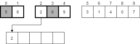
Next, we’ll compare the values 5 and 6, and see that 5 is smaller. It should be placed in the next available element in our temporary array and we should continue onward.
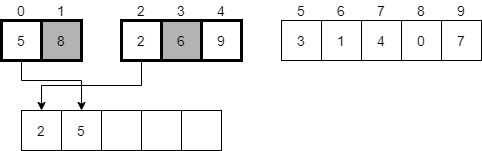
We’ll repeat this process again, placing the 6 in the temporary array, then the 8, then finally the 9. After completing the merge process, we’ll have the following temporary array.
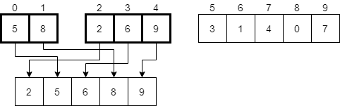
Finally, we’ll replace the original elements with the now merged elements in the temporary array.
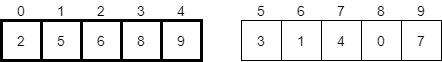
There we go! We’ve now completed the process in the mergeSort(0, 4) recursive call. Once that returns, we’ll be back in our original call to mergeSort(0, 9). In that function, we’ll recursively call the process again on the second half of the array using mergeSort(5, 9).
Hopefully by now we understand that it will work just like we intended, so by the time that recursive call returns, we’ll now have the second half of the array sorted as well.
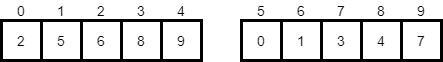
The last step in the original mergeSort(0, 9) function call is to merge these two halves together. So, once again, we’ll follow that same process as before, creating a new temporary array and moving through the elements in each half, placing the smaller of the two in the new array. Once we are done, we’ll end up with a temporary array that has been populated as shown below.
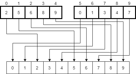
Finally, we’ll replace the elements in the original array with the ones in the temporary array, resulting in a completely sorted result.
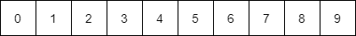
File:Merge-sort-example-300px.gif. (2020, February 22). Wikimedia Commons, the free media repository. Retrieved 00:06, March 24, 2020 from https://commons.wikimedia.org/w/index.php?title=File:Merge-sort-example-300px.gif&oldid=397192885. ↩︎
Now that we’ve seen how merge sort works by going through an example, let’s look at the pseudocode of a merge sort function.
 1function MERGESORT(ARRAY, START, END)
 2    # base case size == 1
 3    if END - START + 1 == 1 then
 4        return
 5    end if
 6    # base case size == 2
 7    if END - START + 1 == 2 then
 8        # check if elements are out of order
 9        if ARRAY[START] > ARRAY[END] then
10            # swap if so
11            TEMP = ARRAY[START]
12            ARRAY[START] = ARRAY[END]
13            ARRAY[END] = TEMP
14        end if
15        return
16    end if
17    # find midpoint
18    HALF = int((START + END) / 2)
19    # sort first half
20    MERGESORT(ARRAY, START, HALF)
21    # sort second half
22    MERGESORT(ARRAY, HALF + 1, END)
23    # merge halves
24    MERGE(ARRAY, START, HALF, END)
25end function
This function is a recursive function which has two base cases. The first base case is shown in lines 3 through 5, where the size of the array is exactly 1. In that case, the array is already sorted, so we just return on line 4 without doing anything.
The other base case is shown in lines 7 through 15. In this case, the element contains just two elements. We can use the if statement on line 9 to check if those two elements are in the correct order. If not, we can use lines 11 through 13 to swap them, before returning on line 15.
If neither of the base cases occurs, then we reach the recursive case starting on line 18. First, we’ll need to determine the midpoint of the array, which is just the average of the start and end variables. We’ll need to remember to make sure that value is an integer by truncating it if needed.
Then, on lines 20 and 22 we make two recursive calls, each one focusing on a different half of the array. Once each of those calls returns, we can assume that each half of the array is now sorted.
Finally, in line 24 we call a helper function known as merge to merge the two halves together. The pseudocode for that process is below.
 1function MERGE(ARRAY, START, HALF, END)
 2    TEMPARRAY = new array[END – START + 1]
 3    INDEX1 = START
 4    INDEX2 = HALF + 1
 5    NEWINDEX = 0
 6    loop while INDEX1 <= HALF and INDEX2 <= END
 7        if ARRAY[INDEX1] < ARRAY[INDEX2] then
 8            TEMPARRAY[NEWINDEX] = ARRAY[INDEX1]
 9            INDEX1 = INDEX1 + 1
10        else
11            TEMPARRAY[NEWINDEX] = ARRAY[INDEX2]
12            INDEX2 = INDEX2 + 1
13        end if
14        NEWINDEX = NEWINDEX + 1
15    end loop
16    loop while INDEX1 <= HALF
17        TEMPARRAY[NEWINDEX] = ARRAY[INDEX1]
18        INDEX1 = INDEX1 + 1
19        NEWINDEX = NEWINDEX + 1
20    end loop
21    loop while INDEX2 <= END
22        TEMPARRAY[NEWINDEX] = ARRAY[INDEX2]
23        INDEX2 = INDEX2 + 1
24        NEWINDEX = NEWINDEX + 1
25    end loop
26    loop INDEX from 0 to size of TEMPARRAY – 1
27        ARRAY[START + INDEX] = TEMPARRAY[INDEX]
28    end loop
29end function
The merge function begins by creating some variables. The tempArray will hold the newly merged array. Index1 refers to the element in the first half that is being considered, while index2 refers to the element in the second half. Finally, newIndex keeps track of our position in the new array.
The first loop starting on line 6 will continue operating until one half or the other has been completely added to the temporary array. It starts by comparing the first element in each half of the array. Then, depending on which one is smaller, it will place the smaller of the two in the new array and increment the indexes.
Once the first loop has completed, there are two more loops starting on lines 16 and 21. However, only one of those loops will actually execute, since only one half of the array will have any elements left in it to be considered. These loops will simply copy the remaining elements to the end of the temporary array.
Finally, the last loop starting on line 26 will copy the elements from the temporary array back into the source array. At this point, they will be properly merged in sorted order.
Now that we’ve reviewed the pseudocode for the merge sort algorithm, let’s see if we can analyze the time it takes to complete. Analyzing a recursive algorithm requires quite a bit of math and understanding to do it properly, but we can get a pretty close answer using a bit of intuition about what it does.
For starters, let’s consider a diagram that shows all of the different recursive calls made by merge sort, as shown below.
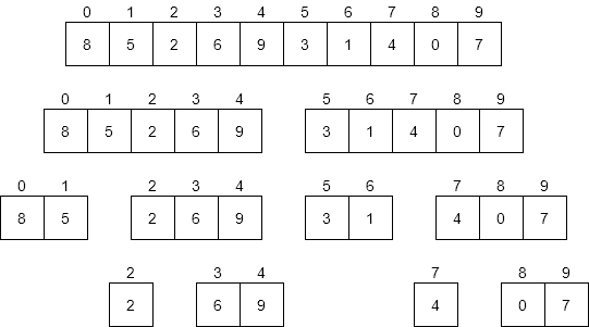
The first thing we should do is consider the worst-case input for merge sort. What would that look like? Put another way, would the values or the ordering of those values change anything about how merge sort operates?
The only real impact that the input would have is on the number of swaps made by merge sort. If we had an input that caused each of the base cases with exactly two elements to swap them, that would be a few more steps than any other input. Consider the highlighted entries below.
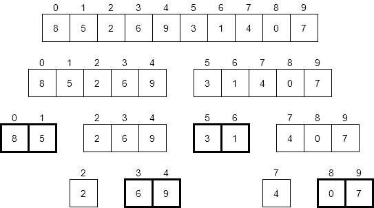
If each of those pairs were reversed, we’d end up doing that many swaps. So, how many swaps would that be? As it turns out, a good estimate would be $N / 2$ times. If we have an array with exactly 16 elements, there are at most 8 swaps we could make. With 10 elements, we can make at most 4. So, the number of swaps is on the order of N time complexity.
What about the merge operation? How many steps does that take? This is a bit trickier to answer, but let’s look at each row of the diagram above. Across all of the calls to merge sort on each row, we’ll end up merging all $N$ elements in the original array at least once. Therefore, we know that it would take around $N$ steps for each row in the diagram. We’ll just need to figure out how many rows there are.
A better way to phrase that question might be “how many times can we recursively divide an array of $N$ elements in half?” As it turns out, the answer to that question lies in the use of the logarithm.
The logarithm is the inverse of exponentiation. For example, we could have the exponentiation formula:
$$ \text{base}^{\text{exponent}} = \text{power} $$The inverse of that would be the logarithm
$$ \text{log}_{\text{base}}(\text{power}) = \text{exponent} $$So, if we know a value and base, we can determine the exponent required to raise that base to the given value.
In this case, we would need to use the logarithm with base $2$, since we are dividing the array in half each time. So, we would say that the number of rows in that diagram, or the number of levels in our tree would be on the order of $\text{log}_2(N)$. In computer science, we typically write $\text{log}_2$ as $\text{lg}$, so we’ll say it is on the order of $\text{lg}(N)$.
To get an idea of how that works, consider the case where the array contains exactly $16$ elements. In that case, the value $\text{lg}(16)$ is $4$, since $2^4 = 16$. If we use the diagram above as a model, we can draw a similar diagram for an array containing $16$ elements and find that it indeed has $4$ levels.
If we double the size of the array, we’ll now have $32$ elements. However, even by doubling the size of the array, the value of $\text{lg}(32)$ is just $5$, so it has only increased by $1$. In fact, each time we double the size of the array, the value of $\text{lg}(N)$ will only go up by $1$.
With that in mind, we can say that the merge operation runs on the order of $N * \text{lg}(N)$ time. That is because there are ${\text{lg}(N)}$ levels in the tree, and each level of the tree performs $N$ operations to merge various parts of the array together. The diagram below gives a good graphical representation of how we can come to that conclusion.

Putting it all together, we have $N/2$ swaps, and $N * \text{lg}(N)$ steps for the merge. Since the value $N * \text{lg}(N)$ is larger than $N$, we would say that total running time of merge sort is on the order of $N * \text{lg}(N)$.
Later on in this chapter we’ll discuss how that compares to the running time of selection sort and bubble sort and how that impacts our programs.
The last sorting algorithm we will review in this module is quicksort. Quicksort is another example of a recursive, divide and conquer sorting algorithm, and at first glance it may look very similar to merge sort. However, quicksort uses a different process for dividing the array, and that can produce some very interesting results.
The basic idea of quicksort is as follows:
pivotValue. This value could be any random value in the array. In our implementation, we’ll simply use the last value.pivotValuepivotValuepivotValue in between those two parts. We’ll call the index of pivotValue the pivotIndex.pivotIndex – 1pivotIndex + 1 to the endAs with all of the other examples we’ve looked at in this module, Wikipedia provides yet another excellent animation showing this process.
Let’s look at an example of the quicksort algorithm in action to see how it works. Unlike the other sorting algorithms we’ve seen, this one may appear to be just randomly swapping elements around at first glance. However, as we move through the example, we should start to see how it achieves a sorted result, usually very quickly!
We can start with our same initial array, shown below.

The first step is to choose a pivot value. As we discussed above, we can choose any random value in the array. However, to make it simple, we’ll just use the last value. We will create two variables, pivotValue and pivotIndex, to help us keep track of things. We’ll set pivotValue to the last value in the array, and pivotIndex will initially be set to 0. We’ll see why in a few steps.
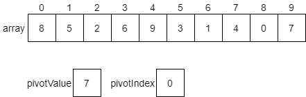
Now, the algorithm will iterate across each element in the array, comparing it with the value in pivotValue. If that value is less than or equal to the pivotValue, we should swap the element at pivotIndex with the value we are looking at in the array. Let’s see how this would work.
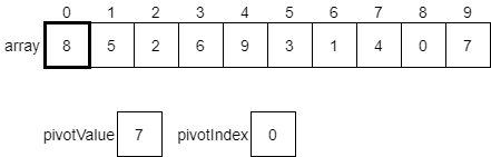
We’d start by looking at the value at index 0 of the array, which is 8. Since that value is greater than the pivotValue, we do nothing and just look at the next item.
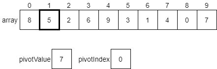
Here, we are considering the value 5, which is at index 1 in the array. In this case, that value is less than or equal to the pivotValue. So, we want to swap the current element with the element at our pivotIndex, which is currently 0. Once we do that, we’ll also increment our pivotIndex by 1. The diagram below shows these changes before they happen.
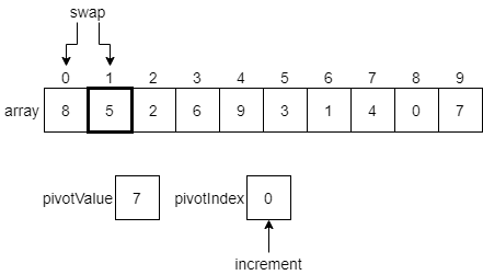
Once we make those changes, our array should look like the following diagram, and we’ll be ready to examine the value at index 2.
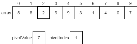
Once again, the value 2 at index 2 of the array is less than or equal to the pivot value. So, we’ll swap them, increment pivotValue, and move to the next element.
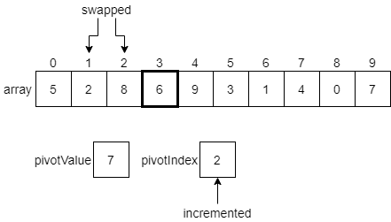
We’ll continue this process, comparing the next element in the array with the pivotValue, and then swapping that element and the element at the pivotIndex if needed, incrementing the pivotIndex after each swap. The diagrams below show the next few steps. First, since 6 is less than or equal to our pivotValue, we’ll swap it with the pivot index and increment.
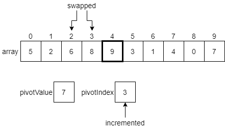
However, since 9 is greater than the pivot index, we’ll just leave it as is for now and move to the next element.
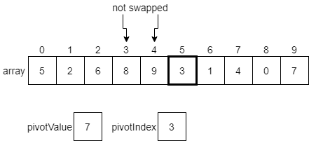
3 is less than or equal to the pivot value, so we’ll swap the element at index 3 with the 3 at index 5.
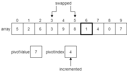
We’ll see that the elements at indexes 6, 7 and 8 are all less than or equal to the pivot value. So, we’ll end up making some swaps until we reach the end of the list.
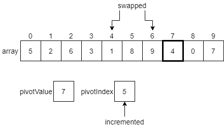
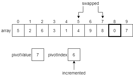
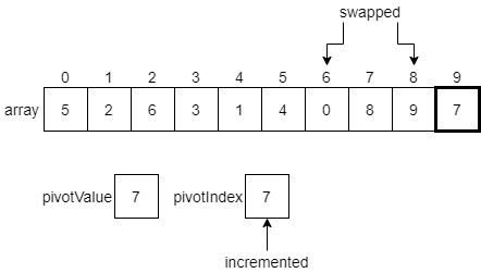
Finally, we have reached the end of the array, which contains our pivotValue in the last element. Thankfully, we can just continue our process one more step. Since the pivotValue is less than or equal to itself, we swap it with the element at the pivotIndex, and increment that index one last time.
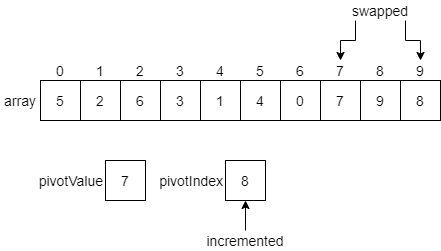
At this point, we have partitioned the initial array into two sections. The first section contains all of the values which are less than or equal to the pivot value, and the second section contains all values greater than the pivot value.
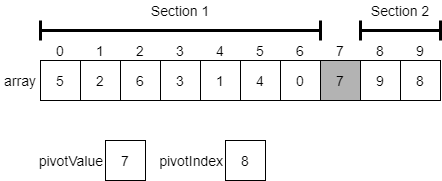
This demonstrates the powerful way that quicksort can quickly partition an array based on a pivot value! With just a single pass through the array, we have created our two halves and done at least some preliminary sorting. The last step is to make two recursive calls to quicksort, one that sorts the items from the beginning of the array through the element right before the pivotValue. The other will sort the elements starting after the pivotValue through the end of the array.
Once each of those recursive calls is complete, the entire array will be sorted!
File:Sorting quicksort anim.gif. (2019, July 30). Wikimedia Commons, the free media repository. Retrieved 01:14, March 24, 2020 from https://commons.wikimedia.org/w/index.php?title=File:Sorting_quicksort_anim.gif&oldid=359998181. ↩︎
Now that we’ve seen an example of how quicksort works, let’s walk through the pseudocode of a quicksort function. The function itself is very simple, as shown below.
1function QUICKSORT(ARRAY, START, END)
2    # base case size <= 1
3    if START >= END then
4        return
5    end if
6    PIVOTINDEX = PARTITION(ARRAY, START, END)
7    QUICKSORT(ARRAY, START, PIVOTINDEX – 1)
8    QUICKSORT(ARRAY, PIVOTINDEX + 1, END)
9end function
This implementation of quicksort uses a simple base case on lines 3 through 5 to check if the array is either empty, or contains one element. It does so by checking if the START index is greater than or equal to the END index. If so, it can assume the array is sorted and just return it without any additional changes.
The recursive case is shown on lines 6 - 8. It simply uses a helper function called partition on line 6 to partition the array based on a pivot value. That function returns the location of the pivot value, which is stored in pivotIndex. Then, on lines 7 and 8, the quicksort function is called recursively on the two partitions of the array, before and after the pivotIndex. That’s really all there is to it!
Let’s look at one way we could implement the partition function, shown below in pseudocode.
 1function PARTITION(ARRAY, START, END)
 2    PIVOTVALUE = ARRAY[END]
 3    PIVOTINDEX = START
 4    loop INDEX from START to END
 5        if ARRAY[INDEX] <= PIVOTVALUE
 6            TEMP = ARRAY[INDEX]
 7            ARRAY[INDEX] = ARRAY[PIVOTINDEX]
 8            ARRAY[PIVOTINDEX] = TEMP
 9            PIVOTINDEX = PIVOTINDEX + 1
10        end if
11    end loop
12    return PIVOTINDEX – 1
This function begins on lines 2 and 3 by setting initial values for the pivotValue by choosing the last element in the array, and then setting the pivotIndex to 0. Then, the loop on lines 4 through 11 will look at each element in the array, determine if it is less than or equal to pivotValue, and swap that element with the element at pivotIndex if so, incrementing pivotIndex after each swap.
At the end, the value that was originally at the end of the array will be at location pivotIndex – 1, so we will return that value back to the quicksort function so it can split the array into two parts based on that value.
To wrap up our analysis of the quicksort algorithm, let’s take a look at the time complexity of the algorithm. Quicksort is a very difficult algorithm to analyze, especially since the selection of the pivot value is random and can greatly affect the performance of the algorithm. So, we’ll talk about quicksort’s time complexity in terms of two cases, the worst case and the average case. Let’s look at the average case first
What would the average case of quicksort look like? This is a difficult question to answer and requires a bit of intuition and making a few assumptions. The key really lies in how we choose our pivot value.
First, let’s assume that the data in our array is equally distributed. This means that the values are evenly spread between the lowest value and the highest value, with no large clusters of similar values anywhere. While this may not always be the case in the real world, often we can assume that our data is somewhat equally distributed.
Second, we can also assume that our chosen pivot value is close to the average value in the array. If the array is equally distributed and we choose a value at random, we have a $50\%$ chance of that value being closer to the average than either the minimum or the maximum value, so this is a pretty safe assumption.
With those two assumptions in hand, we see that something interesting happens. If we choose the average value as our pivot value, quicksort will perfectly partition the array into two equal sized halves! This is a great result, because it means that each recursive call to the function will be working with data that is half the initial array.
If we consider an array that initially contains $15$ elements, and make sure that we always choose the average element as our pivot point, we’d end up with a tree of recursive calls that resembles the diagram below.
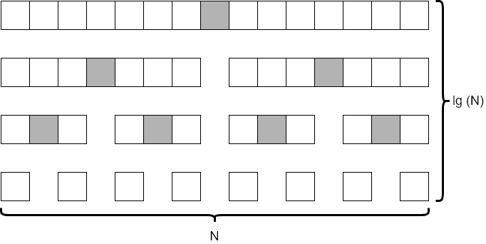
In this diagram, we see that each level of the tree looks at around $N$ elements. (It is actually fewer, but not by a significant amount so we can just round up to $N$ each time). We also notice that there are 4 levels to the tree, which is closely approximated by $\text{lg}(N)$. This is the same result we observed when analyzing the merge sort algorithm earlier in this module.
So, in the average case, we’d say that quicksort runs in the order of $N * \text{lg}(N)$ time.
To consider the worst-case situation for quicksort, we must come up with a way to define what the worst-case input would be. It turns out that the selection of our pivot value is the key here.
Consider the situation where the pivot value is chosen to be the maximum value in the array. What would happen in that case?
Looking at the code, we would see that each recursive call would contain one empty partition, and the other partition would be just one less than the size of the original array. So, if our original array only contained 8 elements, our tree recursion diagram would look similar to the following.
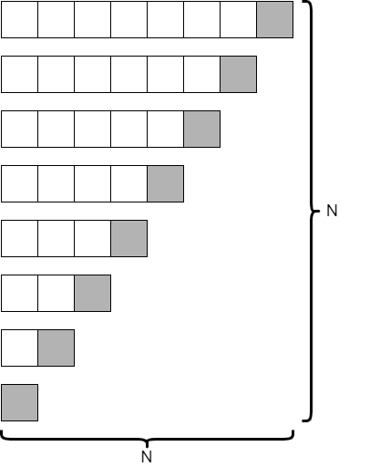
This is an entirely different result! In this case, since we are only reducing the size of our array by 1 at each level, it would take $N$ recursive calls to complete. However, at each level, we are looking at one fewer element. Is this better or worse than the average case?
It turns out that it is much worse. As we learned in our analysis of selection sort and bubble sort, the series
$$ N + (N – 1) + (N – 2) + ... + 2 + 1 $$is best approximated by $N^2$. So, we would say that quicksort runs in the order of $N^2$ time in the worst case. This is just as slow as selection sort and bubble sort! Why would we ever call it “quicksort” if it isn’t any faster?
Thankfully, in practice, it is very rare to run into this worst-case performance with quicksort, and in fact most research shows that quicksort is often the fastest of the four sorting algorithms we’ve discussed so far. In the next section, we’ll discuss these performance characteristics a bit more.
This result highlights why it is important to consider both the worst case and average case performance of our algorithms. Many times we’ll write an algorithm that runs well most of the time, but is susceptible to poor performance when given a particular worst-case input.
We introduced four sorting algorithms in this chapter: selection sort, bubble sort, merge sort, and quicksort. In addition, we performed a basic analysis of the time complexity of each algorithm. In this section, we’ll revisit that topic and compare sorting algorithms based on their performance, helping us understand what algorithm to choose based on the situation.
The list below shows the overall result of our time complexity analysis for each algorithm.
We have expressed the amount of time each algorithm takes to complete in terms of the size of the original input $N$. But how does $N^2$ compare to $N * \text{lg}(N)$?
One of the easiest ways to compare two functions is to graph them, just like we’ve learned to do in our math classes. The diagram below shows a graph containing the functions $N$, $N^2$, and $N * \text{lg}(N)$.
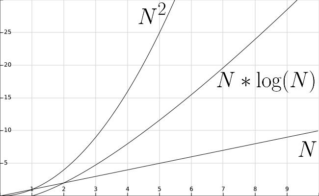
First, notice that the scale along the X axis (representing values of $N$) goes from 0 to 10, while the Y axis (representing the function outputs) goes from 0 to 30. This graph has been adjusted a bit to better show the relationship between these functions, but in actuality they have a much steeper slope than is shown here.
As we can see, the value of $N^2$ at any particular place on the X axis is almost always larger than $N * \text{lg}(N)$, while that function’s output is almost always larger than $N$ itself. We can infer from this that functions which run in the order of $N^2$ time will take much longer to complete than functions which run in the order of $N * \text{lg}(N)$ time. Likewise, the functions which run in the order of $N * \text{lg}(N)$ time themselves are much slower than functions which run in linear time, or in the order of $N$ time.
Based on that assessment alone, we might conclude that we should always use merge sort! It is guaranteed to run in $N * \text{lg}(N)$ time, with no troublesome worst-case scenarios to consider, right? Unfortunately, as with many things in the real world, it isn’t that simple.
The choice of which sorting algorithm to use in our programs largely comes down to what we know about the data we have, and how that information can impact the performance of the algorithm. This is true for many other algorithms we will write in this class. Many times there are multiple methods to perform a task, such as sorting, and the choice of which method we use largely depends on what we expect our input data to be.
For example, consider the case where our input data is nearly sorted. In that instance, most of the items are in the correct order, but a few of them, maybe less than $10\%$, are slightly out of order. In that case, what if we used a version of bubble sort that was optimized to stop sorting as soon as it makes a pass through the array without swapping any elements? Since only a few elements are out of order, it may only take a few passes with bubble sort to get them back in the correct places. So even though bubble sort runs in $N^2$ time, the actual time may be much quicker.
Likewise, if we know that our data is random and uniformly distributed, we might want to choose quicksort. Even though quicksort has very slow performance in the worst case, if our data is properly random and distributed, research shows that it will have better real-world performance than most other sorting algorithms in that instance.
Finally, what if we know nothing about our input data? In that case, we might want to choose merge sort as the safe bet. It is guaranteed to be no worse than $N * \text{lg}(N)$ time, even if the input is truly bad. While it might not be as fast as quicksort if the input is random, it won’t run the risk of being slow, either.
Now that we’ve learned how to sort the data in our container, let’s go back and revisit the concept of searching once again. Does our approach change when we know the data has been sorted?
Our intuition tells us that it should. Recall that we discussed how much easier it would be to find a particular paper in a sorted filing cabinet rather than just searching through a random pile of papers on the floor. The same concept applies to data in our programs.
The most commonly used searching algorithm when dealing with sorted data is binary search. The idea of the algorithm is to compare the value in the middle of the container with the value we are looking for. In this case, let’s assume the container is sorted in ascending order, so the smaller elements are before the larger ones. If we compare our desired value with the middle value, there are three possible outcomes:
Once an occurrence of the desired value is found, we can also look at the values before it to see if there any more of the desired values in the container. Since it is sorted, they should all be grouped together. If we want our algorithm to return the index of the first occurrence of the desired value, we can simply move toward the front of the array until we find that first occurrence.
Let’s work through a quick example of the binary search algorithm to see how it works in practice. Let’s assume we have the array shown in the diagram below, which is already sorted in ascending order. We wish to find out if the array contains the value 5. So, we’ll store that in our value variable. We also have variables start and end representing the first and last index in the array that we are considering.
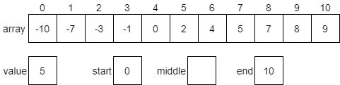
First, we must calculate the middle index of the array. To do that, we can use the following formula.
$$ \text{int}((\text{start} + \text{end}) / 2) $$In this case, we’ll find that the middle index is 5.

Next, we’ll compare our desired value with the element at the middle index, which is 2. Since our desired value 5 is greater than 2, we know that 5 must be present in the second half of the array. We will then update our starting value to be one greater than the middle element and start over. In practice, this could be done either iteratively or recursively. We’ll see both implementations later in this section. The portion of the array we are ignoring has been given a grey background in the diagram below.
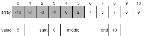
Once again, we’ll start by calculating a new middle index. In this case, it will be 8.

The value at index 8 is 7, which is greater than our desired value 5. So we know that 5 should be in the first half of the array from index 6 through 10. We need to update the end variable to be one less than middle and try once again.

We’ll first calculate the middle index, which will be 6. This is because (6 + 7) / 2 is 6.5, but when we convert it to an integer it will be truncated, resulting in just 6.
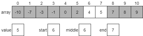
Since the value at index 6 is 4, which is less than our desired value 5, we know that we should be looking at the portion of the array which comes after our middle element. Once again, we’ll update our start index to be one greater than the middle and start over.
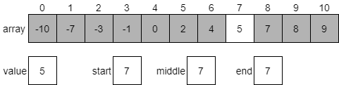
In this case, since both start and end are the same, we know that the middle index will also be 7. We can compare the value at index 7 to our desired value. As it turns out, they are a match, so we’ve found our value! We can just return middle as the index for this value. Of course, if we want to make sure it is the first instance of our desired value, we can quickly check the elements before it until we find one that isn’t our desired value. We won’t worry about that for now, but it is something that can easily be added to our code later.
The binary search algorithm is easily implemented in both an iterative and recursive function. We’ll look at both versions and see how they compare.
The pseudocode for an iterative version of binary search is shown below.
 1function BINARYSEARCH(ARRAY, VALUE)
 2    START = 0
 3    END = size of ARRAY - 1
 4    loop while START <= END
 5        MIDDLE = INT((START + END) / 2)
 6        if ARRAY[MIDDLE] == VALUE then
 7            return MIDDLE
 8        else if ARRAY[MIDDLE] > VALUE then
 9            END = MIDDLE – 1
10        else if ARRAY[MIDDLE] < VALUE then
11            START = MIDDLE + 1
12        end if
13    end loop
14    return -1
15end function
This function starts by setting the initial values of start and end on lines 2 and 3 to the first and last indexes in the array, respectively. Then, the loop starting on line 4 will repeat while the start index is less than or equal to the end index. If we reach an instance where start is greater than end, then we have searched the entire array and haven’t found our desired value. At that point the loop will end and we will return -1 on line 14.
Inside of the loop, we first calculate the middle index on line 5. Then on line 6 we check to see if the middle element is our desired value. If so, we should just return the middle index and stop. It is important to note that this function will return the index to an instance of value in the array, but it may not be the first instance. If we wanted to find the first instance, we’d add a loop at line 7 to move forward in the array until we were sure we were at the first instance of value before returning.
If we didn’t find our element, then the if statements on lines 8 and 10 determine which half of the array we should look at. Those statements update either end or start as needed, and then the loop repeats.
The recursive implementation of binary search is very similar to the iterative approach. However, this time we also include both start and end as parameters, which we update at each recursive call. The pseudocode for a recursive binary search is shown below.
 1function BINARYSEARCHRECURSE(ARRAY, VALUE, START, END)
 2    # base case
 3    if START > END then
 4        return -1
 5    end if
 6    MIDDLE = INT((START + END) / 2)
 7    if ARRAY[MIDDLE] == VALUE then
 8        return MIDDLE
 9    else if ARRAY[MIDDLE] > VALUE then
10        return BINARYSEARCHRECURSE(ARRAY, VALUE, START, MIDDLE – 1)
11    else if ARRAY[MIDDLE] < VALUE then
12        return BINARYSEARCHRECURSE(ARRAY, VALUE, MIDDLE + 1, END)
13    end if
14end function
The recursive version moves the loop’s termination condition to the base case, ensuring that it returns -1 if the start index is greater than the end index. Otherwise, it performs the same process of calculating the middle index and checking to see if it contains the desired value. If not, it uses the recursive calls on lines 10 and 12 to search the first half or second half of the array, whichever is appropriate.
Analyzing the time complexity of binary search is similar to the analysis done with merge sort. In essence, we must determine how many times it must check the middle element of the array.
In the worst case, it will continue to do this until it has determined that the value is not present in the array at all. Any time that our array doesn’t contain our desired value would be our worst-case input.
In that instance, how many times do we look at the middle element in the array? That is hard to measure. However, it might be easier to measure how many elements are in the array each time and go from there.
Consider the situation where we start with 15 elements in the array. How many times can we divide the array in half before we are down to just a single element? The diagram below shows what this might look like.
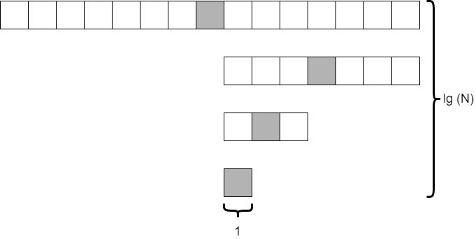
As it turns out, this is similar to the analysis we did on merge sort and quick sort. If we divide the array in half each time, we will do this $\text{lg}(N)$ times. The only difference is that we are only looking at a single element, the shaded element, at each level. So the overall time complexity of binary search is on the order of $\text{lg}(N)$. That’s pretty fast!
Let’s go back and look at the performance of our sorting algorithms, now that we know how quickly binary search can find a particular value in an array. Let’s add the function $\text{lg}(N)$ to our graph from earlier, shown below.

As we can see, the function $\text{lg}(N)$ is even smaller than $N$. So performing a binary search is much faster than a linear search, which we already know runs in the order of $N$ time.
However, performing a single linear search is still faster than any of the sorting algorithms we’ve reviewed. So when does it become advantageous to sort our data?
This is a difficult question to answer since it depends on many factors. However, a good rule of thumb is to remember that the larger the data set, or the more times we need to search for a value, the better off we are to sort the data before we search.
In the graph below, the topmost line colored in red shows the approximate running time of $10$ linear search operations, while the bottom line in black shows the running time of performing a merge sort before $10$ binary search operations.
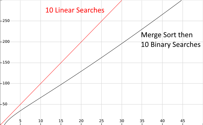
As we can see, it is more efficient to perform a merge sort, which runs in $N * \text{lg}(N)$ time, then perform $10$ binary searches running in $\text{lg}(N)$ time, than it is to perform $10$ linear searches running in $N$ time. The savings become more pronounced as the size of the input gets larger, as indicated by the X axis on the graph.
In fact, this analysis suggests that it may only take as few as 7 searches to see this benefit, even on smaller data sets. So, if we are writing a program that needs to search for a specific value in an array more than about 7 times, it is probably a good idea to sort the array before doing our searches, at least from a performance standpoint.
So far we’ve looked at sorting algorithms that run in $N * \text{lg}(N)$ time. However, what if we try to sort the data as we add it to the array? In a later course, we’ll learn how we can use an advanced data structure known as a heap to create a sorted array in nearly linear time (with some important caveats, of course)!
In this chapter, we learned how to search for values in an array using a linear search method. Then, we explored four different sorting algorithms, and compared them based on their time complexity. Finally, we learned how we can use a sorted array to perform a faster binary search and saw how we can increase our performance by sorting our array before searching in certain situations.
Searching and sorting are two of the most common operations performed in computer programs, and it is very important to have a deep understanding of how they work. Many times the performance of a program can be improved simply by using the correct searching and sorting algorithms to fit the program’s needs, and understanding when you might run into a particularly bad worst-case input.
The project in this module will involve implementing several of these algorithms in the language of your choice. As we learn about more data structures, we’ll revisit these algorithms again to discuss how they can be improved or adapted to take advantage of different structures.
Mergesort iterative without a stack
Quicksort iterative with a stack
Bubble sort recursive
Maps, Hash Tables, and Dictionaries!
A hash table is an unordered collection of key-value pairs, where each key is unique. The great thing about hash tables is that they provide efficient insertion, removal and lookup operations that arrays and linked lists cannot match, such as:
A hash table consists of three components:
A user basically stores a key-value pair in the hash table where the key is used to identify the key-value pair as well as compute where it will be stored. For instance, if we consider all the students in a university, we can store student information (name, address, phone, major, GPA, courses, etc.) in the hash table using their name as the key. Storing a key-value pair in a hash table uses the following procedure.

Retrieving a key-value pair from the hash table follows a similar procedure.
Ideally, it would be nice if there was only a single key-value pair stored in each bucket. However, we cannot guarantee this so we use a linked list to allow us to store multiple items whose key produces the same index.
Another data type that is similar to hash tables and is built into many modern programming languages, is the dictionary or an associative array. A dictionary is a collection of key-value pairs that is directly indexed by a key instead of an integer. These keys can be an integer, a string, or other data types. Dictionaries typically support the following operations:
As you can see dictionaries and hash tables are very similar in their basic operation. However, an important difference is that hash tables tend to allow any type of objects as the value in the key-value pairs, while dictionaries typically require a specific type of object to be the value. A dictionary can be implemented using a variety of data structures including linked lists and hash tables.
As stated previously, a hash table has three main components: an array, a hash function, and a set of buckets that store key-value pairs. We discuss the implementation of these below.
We use an array to hold pointers to the buckets where the key-value pairs are stored. While the array itself is a common data type found in almost every language, there are some important aspects to the arrays used in hash tables.
First, the array must be large enough to store our key-value pairs without too many collisions. A collision occurs when two key-value pairs map to the same array index. Although we cannot keep this from happening, the fewer collisions, the faster the hash table. Thus, the larger the array, the lower the chance for collisions. We capture the size of the array as its capacity.
In the example below, both hash tables are storing the same number of key-value pairs. However, the capacity of the array on the right is more than twice as large as the one on the left. To retrieve a random key-value pair from each of these arrays requires a search of one of the linked list buckets. For the array on the left, the average number of nodes searched is $1.8$, while for the array on the right it is only $1.2$. Thus, in this example doubling the capacity of our array provides a $33\%$ reduction in the time required to retrieve a key-value pair. (Note that these statistics were computed based on these particular array capacities and the number of key-value pairs in the example.)

Second, the array should be re-sizable. Since we generally do not know in advance how many key-value pairs we have to store in our hash table, we need to be able to resize our array when the number of key-value pairs reaches a predefined threshold. This threshold is based on the loading factor, which we define next.
As we store more key-value pairs in a hash table, the number of collisions will increase. The more collisions we have, the less efficient our hash table will become. Thus, at some point, it makes sense to increase the capacity of the array and rehash our table, which means we compute new indexes for all key-value pairs and add them into the new array. The question is, when is the appropriate time to do this?
Traditionally, we answer this question using a ratio of the capacity of the hash table array to the number of key-value pairs stored in the table. There are three key properties of hash tables that come into play here:
Typically, when the load factor reaches a specified threshold, we double the capacity of the array and then rehash the table using the new array. The load factor threshold we choose is a tradeoff between space and time. The larger the array, the more memory you use, but with fewer collisions. Obviously, using a smaller array increases the number of collisions as well as the time it takes to retrieve key-value pairs from the table. For our examples below, we use the standard default load factor of $0.75$.
If our array was large enough to ensure our hash function would compute a unique index for each key (i.e., there would be absolutely no collisions), we could store the key-value pairs directly in the array. Unfortunately, this is almost never the case and collisions do occur. Therefore, we store the key-value pairs in buckets associated with each array index. Buckets are the general term we use to describe the mechanism we use to store key-value pairs and handle any collisions that occur. As shown in the figure below, we use linked lists to implement our buckets, which is a fairly standard approach.

As we recall, linked lists provide constant time operations for adding key-value pairs to the list and linear time operations for retrieving key-value pairs from the list. While linear time seems slow for adding a key-value pair to the list, we need to remember that we are talking only about the number of key-value pairs in a specific list, not the total number of key-value pairs in the entire hash table. Thus, as shown in the figure above, the maximum number of key-value pairs in any linked list is $2$, even though the size of the entire table is $9$. With a load factor of $0.75$ and a good quality hash function that distributes key-value pairs uniformly across the array, our linked lists generally have a small number of items ($2$ or $3$ maximum) in each list. So, even though retrieving is not technically constant time, because it is very close to it in practice, we say that it is.
A hash function converts a key into a hash code, which is an integer value that can be used to index our hash table array. Obviously, there are some hash functions that are better than others. Specifically, a good hash function is both easy to compute and should uniformly distribute the keys across our hash table array. Both of these are important factors in how fast our hash table operates, since we compute a hash code each time we insert or get a key-value pair from the hash table. If it takes too long to compute the hash code, we lose the benefits of having constant time insertion and retrieval operations. Likewise, if the function does not distribute the keys evenly across the table, we end up with several keys in the same bucket, which causes longer times to retrieve key-value pairs.
A good hash function should have three important properties.
Luckily, many modern programming languages provide native support for hash functions. Both Java and Python provide built-in hashing functions. These functions take any object and produce an integer, which we then use with the modulo operator to reduce it to the appropriate size for our array capacity. An example of how to use the Java hashCode function is shown below. More information on the Java hashCode function can be found here.
public int computeIndex(Object key){
    return key.hashCode() % this.getCapacity();
}
An example of using Python’s hash function is shown below. More information on hashing in Python and the hash function can be found here.
def compute_index(self, key):
return hash(key) % self.capacityAnother interesting use of hash functions deals with storing and verifying passwords. When we sign up for an account on a website, it asks us for a password that we’d like to use. Obviously, if that website just stored the password directly in their database, it could be a huge security problem if someone was able to gain access to that information. So, how can the website store a password in a way that prevents a hacker from learning our password, but the website can verify that we’ve entered the correct password?
In many cases, we can use a hash function to do just that. When we first enter our password, the website calculates the hash code for the password and then stores the result in the database.
Then, when we try to log in to the website in the future, we provide the same password, and the website is able to calculate the hash again and verify that they match. As long as the hash function is properly designed, it is very unlikely for two passwords to result in the same hash, even if they are very similar.
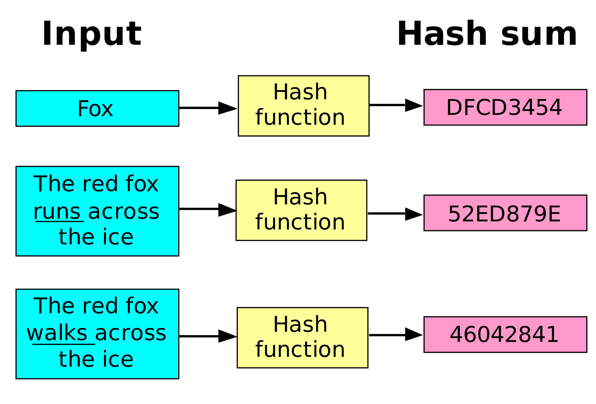
In practice, most websites add additional random data to the password before hashing it, just to decrease the chances of two passwords hashing to the same value. This is referred to as “salting” the password.
Keys allow us to easily differentiate between data items that have different values. For example, if we wanted to store student data such as first name, last name, date of birth, and identification number, it would be convenient to have one piece of data that could differentiate between all the students. However, some data are better suited to be keys than others. In general, the student’s last name tends to be more selective than the first name. However, the student identification number is even better since it is guaranteed to be unique. When a key is guaranteed to be unique, we call them primary keys. The efficiency of a key is also important. Numeric keys are more efficient than alphanumeric keys since computing hash codes with numbers is faster than computing them with characters.
Before we can start describing the basic hash table functions, we first need to create a way to handle key-value pairs. We generally refer to any piece of data that has two parts as a tuple. In the case of key-value pairs, our tuple would look like (key, value). Some languages, such as Python, provide built-in support for creating tuples, while others such as Java and C# require us to create our own tuple class, which is easy to do. All we really need our tuple class to do is to allow us to:
The pseudocode for the Tuple class is given below. Each of the operations is simple and thus we do not discuss them individually. However, notice that the class has two attributes, key and value, that are created in the constructor. The getKey and getValue operations are used often in the code below to provide access to the internals of the tuples.
class Tuple
    object key = null
    object value = null

    function Tuple(object k, object v)
        key = k
        value = v
    end function

    function getKey() returns string
        return key
    end function

    function getValue() returns object
        return value
    end function

    function toString() returns string
        return "(" + key.toString() + "," + value.toString() + ")"
    end function

    function equals(Object o) returns boolean
        if o is not an instance of Tuple:
            return false
        end if
        Tuple t = (Tuple)o
        return (o.key == key) AND (o.value == value)
end functionYou won’t be asked to implement any of these operations since we will just use the built-in class in our chosen language. However, we want you to se behind the scenes and understand how a hash table is implemented directly in code.
The HashTable class has three attributes that provide the basic data structure and parameters we need to efficiently manage our table.
size - captures the number of tuples stored in the table. It is initialized to 0 in line 11 of the constructor.loadFactor - is the load factor used to determine when to increase the capacity of the array. It is initialized to 0.75 in line 12 of the constructor.hashTable - is an array of doubly linked lists. The array is actually created in line 7 of the constructor and the doubly linked lists for each location in the array are created in the loop in lines 8 and 9 of the constructor. 1class HashTable
2 int size
3 double loadFactor = 0.75
4 doubleLinkedList[] hashTable
5
6 function HashTable()
7 hashTable = new doubleLinkedList[16]
8 for i = 0 to hashTable.length
9 hashTable[i] = new doubleLinkedList()
10 end for
11 size = 0
12 loadFactor = 0.75
13 end functionWe assume we are using the language-specific hash code function to actually generate our hash code. However, we need to convert that number (typically a very large integer) to an index for our array, which has a limited capacity. Therefore, we use the modulo function in line 2 to convert the hash code into the range of 0 to the capacity of the array. The computeIndex operation runs in constant time.
1function computeIndex(object key) returns integer
2    return hashCode(key) % getCapacity()
3end functionThe put operation is an important hash table operation, whose goal is to place a key-value pair into the right linked list. We start by calling computeIndex to find which linked list we should store the key-value pair in, which we can access using hashTable[index]. Next, we check to see if the key has already been stored in the table by iterating through the list found at that location in the table. If the key has already been stored, we should update the value in that tuple to be the new value in line 9 and return on line 10. If the key isn’t found, then we actually store the key-value pair in the table by calling the append operation for the hashTable[index] linked list on line 15. Notice, we create a new Tuple using the key and value input parameters before we call append. Since we successfully added the new tuple, we increment the size attribute to keep track of the number of tuples stored in the table.
 1function put(object key, object value)
 2    index = computeIndex(key)
 3
 4    hashTable[index].reset()
 5    current = hashTable[index].getNext()
 6
 7    while current != null
 8        if current.key ==  key
 9            current.value = value
10            return
11        end if
12        current = hashTable[index].getNext()
13    end while
14
15    hashTable[index].append(new Tuple(key, value))
16    size = size + 1
17
18    if size/capacity > loadFactor
19        doubleCapacity()
20    end if
21end function
Since we have added a new tuple to the table, we need to check to see if the size of the table exceeds our load factor. Therefore, in line 18, we check to see if the value of size/capacity exceeds our loadFactor. If it does, we call the doubleCapacity operation to double the capacity of our array and rehash the table. The doubleCapacity operation is defined below.
Since we are looping through a list of elements in the hash table, it can be difficult to analyze the running time of this method. So, we have to look at both the best case and worst case scenario. In the best case, the linked list is empty, so the entire operation runs in constant time. As long as we have a good hash function and the keys are equally distributed across the hash table, this should be the case.
However, if the hash function is poor, it could cause all of the elements in the hash table to be placed in the same list. In that case, the operation would run on the order of $N$ time, since it would have to iterate across all elements in the list.
The get operation is another important hash table operation, whose goal is to retrieve (without deleting) a key-value pair from the table. Like the put operation, the first thing we need to do is to compute the index of the key we are looking for in line 2. Once we know the index, we call the reset operation on the hashTable[index] linked list so we can call the getNext iterator function in line 4. Lines 6 - 8 are a loop that walks through each key-value pair in the linked list. If we find the key we are looking for in line 7, we return true and the operation ends. If we do not find the key, we call the getNext function to get the next element in the linked list. If we end up going through the entire loop until current != null becomes false, we fall out of the loop and return null in line 13, indicating that we did not find key in the table.
 1function get(object key) returns object
 2    index = computeIndex(key)
 3    hashTable[index].reset()
 4    current = hashTable[index].getNext()
 5
 6    while current != null
 7        if current.key ==  key
 8            return current.value
 9        end if
10        current = hashTable[index].getNext()
11    end while
12
13    return null
14end function
As discussed above, although we do end up looping through one of the linked lists in the hash table, these lists are much, much smaller than the overall size of the hash table under most normal circumstances. Thus, we say that the get operation runs in constant time in the best case.
The remove operation is much like the get operation above, except that when we find the key we are searching for, we remove the key-value pair from the appropriate linked-list and return the value to the calling function. The only real difference in the operations lies in the loop intervals in lines 8 and 9. Here, when we find the key in the list, we call the removeCurrent operation to remove the key-value pair from the linked list and then decrement size by 1. Line 10 then returns current.value.
 1function remove(object key) returns object
 2    index = computeIndex(key)
 3    hashTable[index].reset()
 4    current = hashTable[index].getNext()
 5
 6    while current != null
 7        if current.key == key
 8            hashTable[index].removeCurrent()
 9            size = size – 1
10            return current.value
11        end if
12        current = hashTable[index].getNext()
13    end while
14
15    return null
16end function
Like the get operation above, we loop through one of the linked lists in the hash table. However, given the relatively small size of the list, we assume the remove operation runs in constant time in the best case.
The containsKey operation returns a Boolean value based on whether we find the requested key in the table. Since the get operation already finds the key-value pair associated with a given key, we simply call get and then compute whether the key-value pair returned from get exists to compute the containsKey return value. The containsKey operation runs in constant time in the best case.
1function containsKey(object key) returns boolean
2    return get(key) != null
3end functionThe containsValue operation is not as simple as containsKey since we don’t already have an operation to use to search for a value in our hash table. Since we are not given a key to search for, we cannot use the computeIndex to tell us which linked list to search for our value. Therefore, we need to start at the beginning of our array and loop through each element, searching each of the linked lists stored there for our value.
Line 1 is our outside loop that walks through each linked list stored in our array. Within that loop, we follow the same search process we used in the get operation to search through hashTable[i]. We set up the iterator in lines 3 and 4 and then walk through the linked list in the loop in lines 6 - 9. The only difference in this search process is what we are searching for. In line 7, instead of checking if the keys are equal, we check to see if the values are equal. If they are, we return true. However, if we do not find the value somewhere in the table, we must search through every key-value pair in the table, thus the time complexity for containsValue is order $N$.
 1function containsValue(object value) returns boolean
 2    for i = 0 to getCapacity()
 3        hashTable[i].reset()
 4        current = hashTable[i].getNext()
 5
 6        while current != null
 7            if current.value == value
 8                return true
 9            current = hashTable[i].getNext()
10        end while
11    end for
12
13    return false
14end functionThe getSize function is very simple. It simply returns the HashTable class’ size attribute.
1function getSize() returns integer
2    return size
3end functionLike the getSize function, getCapacity simply returns the length of the hashTable array.
1function getCapacity() returns integer
2    return length of the hashTable array
3end functionThe isEmpty operation simply returns the Boolean value of whether or not the size attribute is 0.
1function isEmpty() returns boolean
2    return size == 0
3end functionThe copy operation is similar to the containsValue operation in that it must walk through the entire hash table to get all the key-value pairs in the table and put them into the new hash table. Line 2 creates the new empty hash table, which we call copy.
The for loop in line 4 walks through the hashTable array, allowing us to access each linked list using hashTable[i]. Within the loop we use the linked list iterator functions (lines 5, 6, and 10) to walk through each key-value pair in the linked lists. For each key-value pair, we call copy.put to insert that key-value pair into the copy hash table. Once we have completed both loops, we return the copy in line 14. Like the containsValue operation, since we walk through each key-value pair in the hash table, the copy operation runs in order $N$ time.
 1function copy() returns HashTable
 2    HashTable copy = new HashTable()
 3
 4    for i = 0 to getCapacity()
 5        hashTable[i].reset()
 6        current = hashTable[i].getNext()
 7
 8        while current != null
 9            copy.put(current.key, current.value)
10            current = hashTable[i].getNext()
11        end while
12    end for
13
14    return copy
15end functionThe toString operation is almost identical to the copy operation above, except that instead of inserting each key-value pair into a second hash table, we append the string representation of each key-value pair to an output string. In fact, the only differences to the pseudocode come in lines 2, 9, and 10. Line 2 creates a new empty string and line 13 returns that string after walking through the hash table. Finally, line 9 is where we append the current key-value pair’s string representation to the output string. We also append a comma to separate the key-value pairs in output. Like the copy operation, the toString operation runs in order $N$ time.
 1function toString() returns string
 2    string output = null
 3
 4    for i = 0 to getCapacity()
 5        hashTable[i].reset()
 6        current =  hashTable[i].getNext()
 7
 8        while current != null
 9            output += current.toString() + ", "
10            current =  hashTable[i].getNext()
11        end while
12    end for
13    return output
14end functionThe doubleCapacity operation is similar to the same operations for the array-based stack and queue implementations that we covered earlier. First, we create a new array with twice the capacity of the existing hashTable. Next, we “rehash” each of the key-value pairs in hashTable into the new table. Finally, we point the hashTable attribute at the new table.
The implementation of this process is captured in the following pseudocode. In line 2, we double the size of capacity. It is important to update capacity first so we can use the new value when creating the new hash table array. It is especially important to use this new capacity when calculating the indexes for key-value pairs in the new table.
 1function doubleCapacity()
 2    capacity = capacity * 2
 3    doubleLinkedList[] newTable = new doubleLinkedList[getCapacity()]
 4
 5    for i = 0 to getCapacity()
 6        newTable[i] = new doubleLinkedList()
 7    end for
 8
 9    for i = 0 to getCapacity() / 2
10        hashTable[i].reset()
11        current = hashTable[i].getNext()
12
13        while current != null
14            index = computeIndex(current.key)
15            newTable[index].append(current)
16            current = hashTable[i].getNext()
17        end while
18    end for
19
20    hashTable = newTable
21end function
Line 2 creates a new array called newTable with twice the capacity of the existing table. In lines 5 and 6, we create a new doubly linked list for each element of newTable. Then, in lines 9 - 16 we employ the same looping structure used above in copy and toString to walk through each key-value pair in hashTable. Then for each key-value pair, we compute its new index and then append the key-value pair to the linked list at hashTable[index]. Once we have completed the copying process, we fall out of the loop. Our final action is to point the hashTable attribute at newTable. Like the copy and toString operations, the run time of doubleCapacity is order $N$.
While we do not present the iterator operations here, they are useful operations for hash tables. They are implemented similarly to the other iterator functions we have studied, except that in order to walk through the entire hash table we need to use nested loops where the outside loop walks through the array and the internal loop walks through each linked list. This is very similar to the looping structure in doubleCapacity above.
In this section, we walk through the pseudocode for some basic set operations built on our hash table class above. In this new version of the set class, we declare mySet as a hash table and use that throughout our operations.
mySet = new HashTable()When using a hash table to implement sets, one of the most important choices we must make is what to use for a key. This is really difficult in the case of sets since we do not know exactly what types of objects may be put into the set. Our only real option at this point is just to use the entire object as our key. Our choice to use a default hash function in our hash table turns out to be a good one (at least in modern languages such as Python, Java, and C#), since most default hash functions work on any type of objects.
Next, we discuss the implementation of the important set operations using hash tables.
The contains operation is straightforward since we are using the entire object as the key. We simply return the value from the hash table containsKey operation, which performs the exact function we need.
function contains(object o) returns boolean
    return mySet.containsKey(o)
end functionThe add operation maps almost exactly to the hash table put operation except that the put operation does not return a boolean value. So, we first check to see if the key is already contained in the hash table. If so, we just return false, since we don’t need to add the value to the set. Otherwise, we add a new tuple to the hash table, and then return true.
function add(object o) returns boolean
    if mySet.containsKey(o)
        return false
    end if
    mySet.put(o, o)
    return true
end functionThe set remove operation maps almost exactly to the hash table remove operation, so we just call it and then check to see if the result is not null. If it is null, we will return false since the element was not in the set; otherwise we return true.
function remove(object o) returns boolean
    return mySet.remove(o) != null
end functionThe intersection operation creates a new set that has only elements which exist in both sets under consideration. In code, we basically accomplish this by looping through the elements in one set and then checking to see if they exist in the other set. If they do, then we include them in the intersection.
The pseudocode follows that basic algorithm using the hash table iterator to loop through and look at each element in set1. We start by creating a new set, result, to hold the intersection of set1 and set2 in line 2. Then we get the first element pair from set1 by calling the hash table reset operation in line 2 and the getNext operation in line 3.
 1function intersection(set1, set2) returns set
 2    result = new Set()
 3
 4    set1.reset()
 5    current = set1.getNext()
 6    while current != null
 7        if set2.contains(current.getKey())
 8            result.add(current.getKey())
 9        end if
10        current = set1.getNext()
11    end while
12
13    return result
14end function
Lines 6 - 10 implement the loop that walks through each element in set1. If the current element is contained in set2 (line 7), the operation calls the add operation to insert the key of the current element into the result set. Line 10 gets the next element from set1 and loops back to the top.
Eventually, we look at each element in set1 and fall out of the loop. When that happens, the intersection operation is complete, and it returns the result set in line 13.
The union operation is similar to the intersection operation in that we need to use the hash table iterator operations to walk through our sets. The difference lies in what we include in the new result set. While we only walked through set1 in the intersection operation, picking only those objects that existed in set2, here we start by copying all elements from set2 into the result set and then walk through set1 adding each of its elements to the result set as well. (Here we don’t need to worry about adding duplicates since the add operation takes care of that for us.)
The code starts in line 2 by making a copy of set2 and assigning it to our new result set. Then, lines 4 and 5 reset the set1 iterator and get the first item from set1. Lines 6 - 8 form the while loop that we use to walk through each element in set1. This time, however, we simply add every element we find in line 7 before getting the next object in line 8. Once the loop exists we are done and we return the result set in line 11.
 1function union(set1, set2) returns set
 2    result = set2.copy()
 3
 4    set1.reset()
 5    current = set1.getNext()
 6    while current != null
 7        result.add(current.getKey())
 8        current = set1.getNext()
 9    end while
10
11    return result
12end functionThe isSubset operation below is very much like the intersection operation above as we have a loop in lines 4 - 8 that checks each element of set1 and checks to see if it is in set2. The difference between the two operations is that in the isSubset operation, we do not build a third result set. Instead, if any element in set1 is not found in set2, then we return false since not all elements of set1 are contained in set2. If we get all the way through the loop, we have checked that each element in set1 was found in set2 and we can return true; set1 is a subset of set2.
 1function isSubset (set1, set2) returns boolean
 2    set1.reset()
 3    current = set1.getNext()
 4    while current != null
 5        if set2.contains(current.getKey())
 6            return false
 7        end if
 8        current = set1.getNext()
 9    end while
10
11    return true
12end functionIn this module, we introduced the concept of a hash table, which is a data structure that provides efficient insertion and retrieval operations. We introduced the three essential elements of hash tables:
We then discussed how to implement a hash table class. In our implementation, we chose to use built-in, language-specific hash code functions to generate the indexes into our array. We also used doubly linked lists to implement our buckets as linked lists are very flexible and provide constant time insertion operations. To demonstrate the effectiveness of hash tables, we re-implemented our set class using hash tables instead of linked lists. In many ways, the re-implementation was almost identical to the linked list implementation since many of the operations found in hash tables are almost identical to those found in linked lists. We also noted that the biggest advantage of implementing sets with hash tables is the (almost!) constant time retrieval operations provided by hash tables.
Choosing the correct data structures & writing efficient programs that use strings!
There are several linear data structures that we can use in our programs, including stacks, queues, lists, sets, and hash tables. In this course, we have covered each of these structures in detail. However, as a programmer, one of the most difficult decisions we will make when developing a program is the choice of which data structure to use. Sometimes the choice may be obvious based on the data we plan to store or the algorithms we need to perform, but in practice that happens very rarely. Instead, we are faced with competing tradeoffs between various factors such as ease of use, performance, and simplicity.
In this chapter, we’ll review the various data structures and algorithms we’ve learned about in this course, but this time we’ll add a bit more focus on the decisions a programmer would make when choosing to use a particular data structure or algorithm.
The choice of which data structure to use is often the most consequential choice we make when developing a new piece of software, as it can have a large impact on the overall performance of the program. While there are many different factors to consider, here are three important questions we can ask when choosing a data structure:
By answering the questions above in the order they are presented, we should be able to make good decisions about which data structures would work best in our program. We are purposely putting more focus on writing working and understandable code instead of worrying about performance. This is because many programs are only used with small data sets on powerful modern computers, so performance is not the most important aspect. However, there are instances where performance becomes much more important, and in those cases more focus can be placed on finding the most performant solution as well.
As it turns out, these three questions are very similar to a classic (trilemma)[https://en.wikipedia.org/wiki/Trilemma] from the world of business, as shown in the diagram below.
In the world of software engineering, it is said that the process of developing a new program can only have two of the three factors of “good”, “fast”, and “cheap”. The three questions above form a similar trilemma. Put another way, there will always be competing tradeoffs when selecting a data structure for our programs.
For example, the most performant option may not be as easy to understand, and it may be more difficult to debug and ensure that it works correctly. A great example of this is matrix multiplication, a very common operation in the world of high-performance computing. A simple solution requires just three loops and is very easy to understand. However, the most performant solution requires hundreds of lines of code, assembly instructions, and a deep understanding of the hardware on which the program will be executed. That program will be fast and efficient, but it is much more difficult to understand and debug.
File:Project-triangle.svg. (2020, January 12). Wikimedia Commons, the free media repository. Retrieved 21:09, April 30, 2020 from https://commons.wikimedia.org/w/index.php?title=File:Project-triangle.svg&oldid=386979544. ↩︎
Data structures that are used in our programs can be characterized in terms of two performance attributes: processing time and memory usage.
We will not worry about memory usage at this point, since most of the memory used in these data structures is consumed by the data that we are storing. More technically, we would say that the memory use of a data structure containing N elements is on the order of $N$ size. However, some structures, such as doubly linked lists, must maintain both the next and previous pointers along with each element, so there can be a significant amount of memory overhead. That is something we should keep in mind, but only in cases where we are dealing with a large amount of data and are worried about memory usage.
When evaluating the processing time of a data structure, we are most concerned with the algorithms used to add, remove, access, and find elements in the data structure itself. There are a couple of ways we can evaluate these operations.
Throughout this course, we have included mathematical descriptions of the processing time of most major operations on the data structures we have covered.
One of the best ways to compare data structures is to look at the common operations that they can perform. For this analysis, we’ve chosen to analyze the following four operations:
The following table compares the best- and worst-case processing time for many common data structures and operations, expressed in terms of $N$, the number of elements in the structure.
| Data Structure | Insert Best | Insert Worst | Access Best | Access Worst | Find Best | Find Worst | Delete Best | Delete Worst |
|---|---|---|---|---|---|---|---|---|
| Unsorted Array | $1$ | $1$ | $1$ | $1$ | $N$ | $N$ | $N$ | $N$ |
| Sorted Array | $\text{lg}(N)$ | $N$ | $1$ | $1$ | $\text{lg}(N)$ | $\text{lg}(N)$ | $\text{lg}(N)$ | $N$ |
| Array Stack (LIFO) | $1$ | $1$ | $1$ | $1$ | $N$ | $N$ | $1$ | $1$ |
| Array Queue (FIFO) | $1$ | $1$ | $1$ | $1$ | $N$ | $N$ | $1$ | $1$ |
| Unsorted Linked List | $1$ | $1$ | $N$ | $N$ | $N$ | $N$ | $N$ | $N$ |
| Sorted Linked List | $N$ | $N$ | $N$ | $N$ | $N$ | $N$ | $N$ | $N$ |
| Linked List Stack (LIFO) | $1$ | $1$ | $1$ | $1$ | $N$ | $N$ | $1$ | $1$ |
| Linked List Queue (FIFO) | $1$ | $1$ | $1$ | $1$ | $N$ | $N$ | $1$ | $1$ |
| Hash Table | $1$ | $N$ | $1$ | $N$ | $N$ | $N$ | $1$ | $N$ |
We can also compare these processing times by graphing the equations used to describe them. The graph below shows several of the common orders that we have seen so far.

On the next few pages, we will discuss each data structure in brief, using this table to compare the performance of the various data structures we’ve covered in this course.

The next data structure we learned about is the linked list. Specifically, we will look at the doubly linked list in this example, but in most instances the performance of a singly linked list is comparable.
With a linked list, the process of inserting an element at either the beginning or the end is a constant time operation since we maintain both a head and a tail reference. All we must do is create a new node and update a few references and we are good to go.
However, if we would like to access a specific element somewhere in the list, we will have to iterate through the list starting from either the head or the tail until we find the element we need. So, that operation runs in order $N$ time. This is the major difference between linked lists and arrays: with an array, we can directly access items using the array index, but with linked lists we must iterate to get to that element. This becomes important in the next section when we discuss the performance of a sorted linked list.
Similarly, the process of finding an element also requires iterating through the list, which is an operation that runs in order $N$ time.
Finally, if we want to find and delete an element, that also runs in order $N$ time since we must search through the list to find the element. Once we have found the element, the process of deleting that element is a constant time operation. So, if we use our list iterator methods in an efficient manner, the actual run time may be more efficient than this analysis would lead us to believe.

We have not directly analyzed the performance of a sorted linked list in this course, but hopefully the analysis makes sense based on what we have learned before. Since the process of iterating through a linked list runs in order of $N$ time, every operation required to build a sorted linked list is limited by that fact.
For example, if we want to insert an element into a list in sorted order, we must simply iterate through the list to find the correct location to insert it. Once we’ve found it, the process of inserting is actually a constant time operation since we don’t have to shift any elements around, but because we can’t use binary search on a linked list, we don’t have any way to take advantage of the fact that the list is sorted.
The same problem occurs when we want to search for a particular element. Since we cannot use binary search to jump around between various elements in the list, we are limited to a simple linear search process, which runs in order of $N$ time.
Likewise, when we want to search and delete an element from the list, we must once again iterate through the entire list, resulting in an operation that runs in order $N$ time.
So, is there any benefit to sorting a linked list? Based on this analysis, not really! The purpose of sorting a collection is simply to make searching for a particular element faster. However, since we cannot use array indices to jump around a list like we can with an array, we do not see much of an improvement.
However, in the real world, we can improve some of these linear algorithms by “short-circuiting” them. When we “short-circuit” an algorithm, we provide additional code that allows the algorithm to return early if it realizes that it will not succeed.
For example, if we are searching for a particular element in a sorted list, we can add an if statement to check and see if the current element is greater than the element we are searching for. If the list is sorted in ascending order, we know that we have gone past the location where we expected to find our element, so we can just return without checking the rest of the list. While this does not change the mathematical analysis of the running time of this operation, it may improve the real-world empirical analysis of the operation.
We already saw how to use the operations from a linked list to implement both a stack and a queue. Since those data structures restrict the operations we can perform a bit, it turns out that we can use a linked list to implement a stack and a queue with comparable performance to an array implementation.
For example, inserting, accessing, and removing elements in a stack or a queue based on a doubly linked list are all constant time operations, since we can use the head and tail references in a doubly linked list to avoid the need to iterate through the entire list to perform those operations. In fact, the only time we would have to iterate through the entire list is when we want to find a particular element in the stack or the queue. However, since we cannot sort a stack or a queue, finding an element runs in order $N$ time, which is comparable to an array implementation.
By limiting the actions we want to perform with our linked list, we can get a level of performance similar to an array implementation of a stack or a queue. It is a useful outcome that demonstrates the ability of different data structures to achieve similar outcomes.

Analyzing the performance of a hash table is a bit trickier than the other data structures, mainly due to how a hash table tries to use its complex structure to get a “best of both worlds” performance outcome.
For example, consider the insert operation. In the best case, the hash table has a capacity that is large enough to guarantee that there are not any hash collisions. Each entry in the array of the hash table will be an empty list and inserting an element into an empty list is done in constant time, so the whole operation runs in the order of constant time.
The worst case for inserting an item into a hash table would be when every element has the same hash, so every element in the hash table is contained in the same list. In that case, we must iterate through the entire list to make sure the key has not already been used, which would be in the order of $N$ time.
Thankfully, if we properly design our hash table such that the capacity is much larger than our expected size, and the hash function we use to hash our keys results in a properly distributed hash, this worst case scenario should happen very rarely, if ever. Therefore, our expected performance should be closer to constant time.
One important thing to remember, however, is that each operation in a hash table requires computing the hash of the key given as input. Therefore, while some operations may run in constant time, if the action of computing the hash is costly, the overall operation may run very slowly.
The analysis of the operation to access a single element in a hash table based on a given key is similar. If the hash table elements are distributed across the table, then each list should only contain a single element. In that case, we can just compute the hash of the key and determine if that key has been used in a single operation, which runs in the order of constant time.
In the worst case, however, we once again have the situation where all the elements have been placed in the same linked list. We would need to iterate through each element to find the one we are looking for. In that case, the operation would run in the order of $N$ time.
The operation for finding a specific element in a hash table is a bit unique. In this case, we are discussing looking for a particular value, not necessarily a particular key. That operation is discussed in the previous paragraph. For the operation, the only possible way forward is to iterate through each list in the hash table and perform a linear search for the requested value, which will always run in order $N$ time.
Finally, if we want to delete a single element from a hash table based on a given key, the analysis is the same as inserting or finding an element. In the best case, it runs in the order of constant time, but the worst case runs in the order of N time since we must iterate through an entire list of $N$ elements.
Even though a hash table has some very poor performance in the worst case, as discussed earlier those worst case situations are very rare, and as long as we are careful about how we manage the capacity of our hash table and how we compute the hash of our objects, we can expect to see operations running in near constant time during normal usage.
We can examine the performance of the algorithms we use in a similar manner. Once again, we are concerned with both the memory usage and processing time of the algorithm. In this case, we are concerned with the amount of memory required to perform the algorithm that is above and beyond the memory used to store the data in the first place.
When analyzing searching and sorting algorithms, we’ll assume that we are using arrays as our data structure, since they give us the best performance for accessing and swapping random elements quickly.
There are two basic searching algorithms: linear search and binary search.
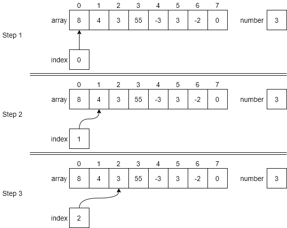
For linear search, we are simply iterating through the entire data structure until we find the desired item. So, while we can stop looking as soon as it is found, in the worst case we will have to look at all the elements in the structure, meaning the algorithm runs in order $N$ time.

Binary search, on the other hand, takes advantage of a sorted array to jump around quickly. In effect, each element we analyze allows us to eliminate half of the remaining elements in our search. With as few as 8 steps, we can search through an array that contains 64 elements. When we analyze this algorithm, we find that it runs in order $\text{lg}(N)$ time, which is a vast improvement over binary search.
Of course, this only works when we can directly access elements in the middle of our data structure. So, while a linked list gives us several performance improvements over an array, we cannot use binary search effectively on a linked list.
In terms of memory usage, since both linear search and binary search just rely on the original data structures for storing the data, the extra memory usage is constant and consists of just a couple of extra variables, regardless of how many elements are in the data structure.
We have already discussed how much of an improvement binary search is over a linear search. In fact, our analysis showed that performing as few as 7 or 8 linear searches will take more time than sorting the array and using binary search. Therefore, in many cases we may want to sort our data. There are several different algorithms we can use to sort our data, but in this course we explored four of them: selection sort, bubble sort, merge sort, and quicksort.
The selection sort algorithm involves finding the smallest or largest value in an array, then moving that value to the appropriate end, and repeating the process until the entire array is sorted. Each time we iterate through the array, we look at every remaining element. In the module on sorting, we showed (through some clever mathematical analysis) that this algorithm runs in the order of $N^2$ time.
Bubble sort is similar, but instead of finding the smallest or largest element in each iteration, it focuses on just swapping elements that are out of order, and eventually (through repeated iterations) sorting the entire array. While doing so, the largest or smallest elements appear to “bubble” to the appropriate end of the array, which gives the algorithm its name. Once again, because the bubble sort algorithm repeatedly iterates through the entire data structure, it also runs on the order of $N^2$ time.
Both selection sort and bubble sort are inefficient as sorting algorithms go, yet their main value is their simplicity. They are also very nice in that they do not require any additional memory usage to run. They are easy to implement and understand and make a good academic example when learning about algorithms. While they are not used often in practice, later in this module we will discuss a couple of situations where we may consider them useful.
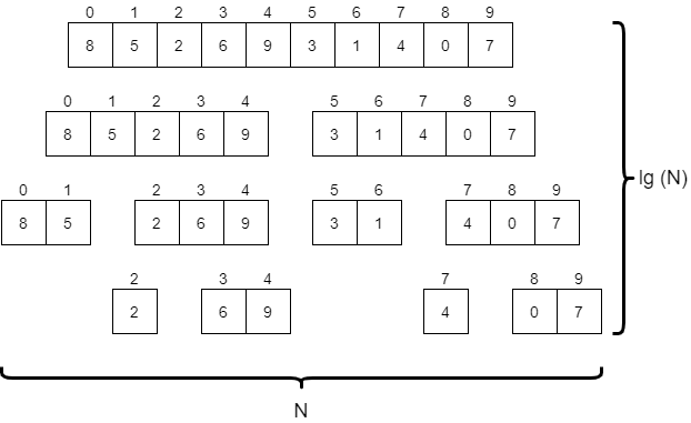
Merge sort is a very powerful divide and conquer algorithm, which splits the array to be sorted into progressively smaller parts until each one contains just one or two elements. Then, once those smaller parts are sorted, it slowly merges them back together until the entire array is sorted. We must look at each element in the array at least once per “level” of the algorithm in the diagram above, so overall this algorithm runs in the order of $N * \text{lg}(N)$ time. This is quite a bit faster than selection sort and bubble sort. However, most implementations of merge sort require at least a second array for storing data as it is merged together, so the additional memory usage is also on the order of $N$.

Quicksort is a very clever algorithm, which involves selecting a “pivot” element from the data, and then dividing the data into two halves, one containing all elements less than the pivot, and another with all items greater than the pivot. Then, the process repeats on each half until the entire structure is sorted. In the ideal scenario, shown in the diagram above, quicksort runs on the order of $N * \text{lg}(N)$ time, similar to merge sort. However, this depends on the choice of the pivot element being close to the median element of the structure, which we cannot always guarantee. Thankfully, in practice, we can just choose a random element (such as the last element in the structure) and we’ll see performance that is close to the $N * \text{lg}(N)$ target.

However, if we choose our pivot element poorly, the worst case scenario shown in the diagram above can occur, causing the run time to be on the order of $N^2$ instead. This means that quicksort has a troublesome, but rare, worst case performance scenario.
There are many different algorithms we can use to sort our data, and some of them can be shown mathematically to be more efficient, even in the worst case. So, how should we choose which algorithm to use?
In practice, it really comes down to a variety of factors, based on the amount of data we expect our program to handle, the randomness of the data, and more. The only way to truly know which algorithm is the best is to empirically test all of them and choose the fastest one, but even that approach relies on us predicting the data that our program will be utilizing.
Instead, here are some general guidelines we can use to help us select a sorting algorithm to use in our program.
Of course, the choice of which sorting algorithm to use is one of the most important decisions a programmer can make, and it is a great example of the fact that there are multiple ways to write a program that performs a particular task. Each possible program comes with various performance and memory considerations, and in many cases, there may not be a correct option. Instead, we must rely on our own knowledge and insight to choose the method that we feel would work best in any given situation.
Throughout this course, we have looked at a few ways we can use the data structures we have already learned to do something useful. In this module, we will look at a few of those examples again, as well as a few more interesting uses of the data structures that we have built.
First and foremost, it is important to understand that we can implement many of the simpler data structures such as stacks, queues and sets using both arrays and linked lists. In fact, from a certain point of view, there are only two commonly used containers for data – the array and the linked list. Nearly all other data structures are a variant of one of those two approaches or a combination of both.
Earlier in this chapter, we discussed some of the performance implications that arise when using arrays or linked lists to implement stacks and queues. In practice, we need to understand how we will be using our data in order to choose between the two approaches.
One unique use of sets appears in the code of compilers and interpreters. In each case, a programming language can only have one instance of a variable with a given name at any one time. So, we can think of the variables in a program as a set. In the code for a compiler or interpreter, we might find many instances of sets that are used to enforce rules that require each variable or function name to be unique.
Of course, this same property becomes important in even larger data storage structures, such as a relational database. For example, a database may include a column for a username or identification number which must be unique, such that no two entries can be the same. Once again, we can use a set to help enforce that restriction.
Hash tables are a great example of a data structure that effectively combines arrays and linked lists to increase performance. The best way to understand this is through the analysis of a set implemented using a hash table instead of a linked list.
When we determine if an element is already contained in a set based on a linked list, we must perform a linear search which runs on the order of $N$ time. The same operation performed on a set based on a hash table runs in constant time in the best case. This is because we can use the result of the hash function to jump directly to the bucket where the item should be stored, if it exists.
This same trick is used in large relational databases. If we have a database with a million rows, we can define an index for a column that allows us to quickly jump to entries without searching the entire database. To look up a particular entry using an index, we can calculate its hash, find the entry in the index, and then use the link in that index element to find the record in the database.
Finally, we can also use hash tables to build efficient indexes for large amounts of text data. Consider a textbook, for example. Most textbooks contain an index in the back that gives the page locations where particular terms are discussed. How can we create that index? We can iterate through each word in the textbook, but for each one we will have to search through the existing words in the index to see if that page is already listed for that word. That can be very slow if we must use a linear search through a linked list. However, if we use a hash table to store the index, the process of updating entries can be done in nearly constant time!
Both Java and Python include standard implementations of each of the data structures we have learned about in this course. While it is very useful and interesting from an academic perspective to build our own linked lists and hash tables, in practice we would rarely do so. In this section, we will briefly introduce the standard library versions of each data structure and provide references to where we can find more information about each one and how to use them.
Python includes many useful data structures as built-in data types. We can use them to build just about any structure we need quickly and efficiently. The Python Tutorial has some great information about data structures in Python and how we can use them.
Python includes several data types that are grouped under the heading of sequence data types, and they all share many operations in common. We’ll look at two of the sequence data types: tuples and lists.
While we have not directly discussed tuples often, it is important to know that Python natively supports tuples as a basic data type. In Python, a tuple is simply a combination of a number of values separated by commas. They are commonly placed within parentheses, but it is not required.
We can directly access elements in a tuple using the same notation we use for arrays, and we can even unpack tuples into multiple variables or return them from functions. Tuples are a great way to pass multiple values as a single variable.
tuple1 = 'a', 'b', 'c'
print(tuple1)  # ('a', 'b', 'c')

tuple2 = (1, 2, 3, 4)
print(tuple2)  # (1, 2, 3, 4)
print(tuple2[0]) # 1
a, b, c, d = tuple2
print(d) # 4Python’s default data structure for sequences of data is the list. In fact, throughout this course, we have been using Python lists as a stand-in for the arrays that are supported by most other languages. Thankfully, lists in Python are much more flexible, since they can be dynamically resized, sliced, and iterated very easily. In terms of performance, a Python list is roughly equivalent to an array in other languages. We can access elements in constant time when the index is known, but inserting and removing from the beginning of the list runs in order of $N$ time since elements must be shifted backwards. This makes them a poor choice for queues and stacks, where elements must be added and removed from both ends of the list.
list1 = ['a', 'b', 'c']
print(list1) # ['a', 'b', 'c']
print(list1[1:2]) # ['b', 'c']The Python Collections library contains a special class called a deque (pronounced “deck”, and short for “double ended queue”) that is a linked list-style implementation that provides much faster constant time inserts and removals from either end of the container. In Python, it is recommended to use the deque data structure when implementing stacks and queues.
In a deque, the ends are referred to as “right” and “left”, so there are methods append() and pop() that impact the right side of the container, and appendleft() and popleft() that modify the left side. We can use a combination of those methods to implement both a Stack and a Queue using a deque in Python.
from collections import deque

# Stack
stack = deque()
stack.append(1)
stack.append(2)
print(stack[-1]) # 2 (peek right side)
print(stack.pop()) # 2
print(stack.pop()) # 1

# Queue
queue = deque()
queue.append(1)
queue.append(2)
print(queue[0]) # 1 (peek left side)
print(queue.popleft()) # 1
print(queue.popleft()) # 2Python also implements a version of the class Map data structure, called a dictionary. In Python, a dictionary stores key-value pairs, very similarly to how associative arrays work in other languages. Behind the scenes, it uses a hashing function to efficiently store and retrieve elements, making most operations run in near constant time.
The one limitation with Python dictionaries is that only hashable data types can be used as keys. We cannot use a list or a dictionary as the key for a dictionary in Python. Thankfully, strings, numbers, and most objects that implement a __hash__() and __eq__() method can be used.
dict = {'name': 123, 'test': 321}
print(dict['name']) # 123 (get a value)
dict['date'] = 456 # (add a new entry)
print('name' in dict) # True (search for entry)Python also includes a built in data type to represent a set. Just like we saw with our analysis, Python also uses a hash-based implementation to allow us to quickly find elements in the set, and therefore does not keep track of any ordering between the elements. We can easily add or remove elements, and Python uniquely allows us to use the binary operators to compute several set operations such as union and intersection.
set1 = {1, 3, 5, 7, 9}
set2 = {2, 3, 5, 7}
print(2 in set1) # False (check for membership)
print(2 in set2) # True (check for membership)

print(set1 – set2) # {1, 9} (set difference)
print(set1 | set2) # {1, 3, 5, 7, 9, 2} (union)
print(set1 & set2) # {3, 5, 7} (intersection)This video was created as part of another course. We have moved this content into CC 310 as a great example of a data structure that exists purely for performance reasons
In CC 310 we covered various data structures: stacks, sets, lists, queues, and hash tables. When we looked at these structures, we considered how to access elements within the structures, how we would create our own implementation of the structure, and tasks that these structures would be fitting for as well as ill fitting. Throughout this course we will introduce and implement a variety of data structures as we did in CC 310.
We begin this course with an often overlooked structure: strings. By the end of this chapter, we will understand how strings are data structures, how we access elements, what types of tasks are appropriate for strings, and how we can improve on strings in our code.
In many data science positions, programmers often work with text-based data. Some examples of text-based data include biology for DNA sequencing, social media for sentiment classification, online libraries for citation networks, and many other types of businesses for data analytics. Currently, strings are often used for word embeddings, which determine how similar or dissimilar words are to one another. An industry leading software for this application is Tensorflow for Python, which generated the image below.
In an immense oversimplification, the process used for word embeddings is to read in a large amount of text and then use machine learning algorithms to determine similarity by using the words around each word. This impacts general users like us in search engines, streaming services, dating applications, and much more! For example, if you were to search Python topics in your search results may appear referring to the coding language, the reptile, the comedy troupe, and many more. When we use machine learning to determine word meanings, it is important that the data is first parsed correctly and stored in efficient ways so that we can access elements as needed. Understanding how to work with strings and problems that can arise with them is important to utilizing text successfully.
Reference: https://projector.tensorflow.org/
Strings are data structures which store an ordered set of characters. Recall that a character can be a: letter, number, symbol, punctuation mark, or white space. Strings can contain any number and any combination of these. As such, strings can be single characters, words, sentences, and even more.
Let’s refresh ourselves on how strings work, starting with the example string: s = "Go Cats!".
| Character | G | o | C | a | t | s | ! | |
| Index | 0 | 1 | 2 | 3 | 4 | 5 | 6 | 7 |
As with other data structures, we can access elements within the string itself. Using the example above, s[0] would contain the character ‘G’, s[1] would contain the character ‘o’, s[2] would contain the character ’ ‘, and so on.
We can determine the size of a string by using length functions; in our example, the length of s would be 8. It is also important to note that when dealing with strings, null is not equivalent to “”. For string s = "", the length of s would be 0. However for string s = null, accessing the length of s would return an error that null has no length property.
We can also add to strings or append on a surface level; though it is not that simple behind the scenes. The String class is immutable. This means that changes will not happen directly to the string; when appending or inserting, code will create a new string to hold that value. More concisely, the state of an immutable object cannot change.
We cannot assign elements of the string directly and more broadly for any immutable object. For example, if we wanted the string from our example to be ‘Go Cat!!’, we cannot assign the element through s[6] = '!'. This would result in an item assignment error.
For an example, consider string s = ‘abc’. If we then state in code s = s + ‘123’, this will create a new place in memory for the new definition of s. We can verify this in code by using the id() function.
string s = 'abc'
id(s)
Output: 140240213073680 #may be different on your personal device

string s = s + '123'
id(s)
Output: 140239945470168
While on the surface it appears that we are working with the same variable, our code will actually refer to a different one. There are many other immutable data types as well as mutable data types.
On the topic of immutable, we can also discuss the converse: mutable objects. Being a mutable object means that the state of the object can change. In CC310, we often worked with arrays to implement various data structures. Arrays are mutable, so as we add, change, or remove elements from an array, the array changes its state to accommodate the change rather than creating a new location in memory.
| Data Type | Immutable? |
|---|---|
| Lists | ☐ |
| Sets | ☐ |
| Byte Arrays | ☐ |
| Dictionaries | ☐ |
| Strings | ☑ |
| Ints | ☑ |
| Floats | ☑ |
| Booleans | ☑ |
Reference: http://people.cs.ksu.edu/~rhowell/DataStructures/strings/strings.html
Consider the following block of pseudocode:
1. function APPENDER(NUMBER, BASE)
2.     RESULT = ""
3.     loop I from 1 to NUMBER
4.         RESULT = RESULT + BASE
5.         if I MOD 2 = 0
6.             RESULT = RESULT + " "
7.         else
8.             RESULT = RESULT + ", "
9.     end loop
10.    return RESULT
11. end function
Lets step through the function call with APPENDER(4,'abc') and analyze the memory that the code takes.
Recall that strings are reference variables. As such, string variables hold pointers to values and the value is stored in memory. For the following example, the HEAP refers to what is currently stored in memory and VARIABLE shows the current value of the variable RESULT.
Initialization: In line two, we initialize RESULT as an empty string. In the heap, we have the empty string at memory location 0x1. Thus, RESULT is holding the pointer 0x1.
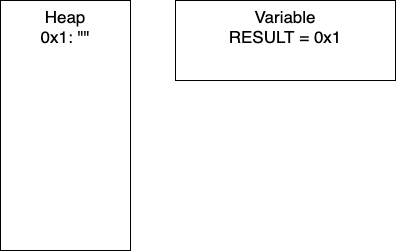
I = 1: Now we have entered the loop and on line 4, we add more characters to our string. At this point, we would have entry 0x2 in our heap and our variable RESULT would have the pointer 0x2. Continuing through the code, line 5 determines if I is divisible by 2. In this iteration I = 1, so we take the else branch. We again add characters to our string, resulting in a new entry in 0x3 and our variable RESULT containing the pointer 0x3. In total, we have written 8 characters. We then increment I and move to the next iteration.
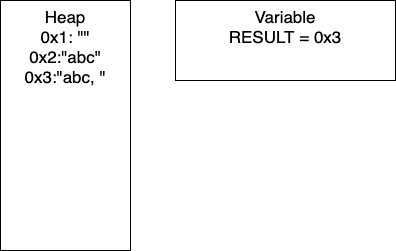
I = 2: We continue the loop and on line 4, we add more characters to our string. At this point, we would have entry 0x4 in our heap and our variable RESULT would have the pointer 0x4. Continuing through the code, line 5 determines if I is divisible by 2. In this iteration I = 2, so we take the if branch. We again add characters to our string, resulting in a new entry in 0x5 and our variable RESULT containing the pointer 0x5. In this iteration, we have written 17 characters. We then increment I and move to the next iteration of the loop.
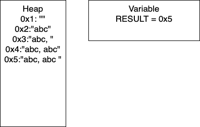
I = 3: We continue the loop and on line 4, we add more characters to our string. At this point, we would have entry 0x6 in our heap and our variable RESULT would have the pointer 0x6. Continuing through the code, line 5 determines if I is divisible by 2. In this iteration I = 3, so we take the if branch. We again add characters to our string, resulting in a new entry in 0x7 and our variable RESULT containing the pointer 0x7. In this iteration, we have written 26 characters. We then increment I and thus I = 4 breaking out of the loop.
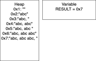
We can do some further analysis of the memory that is required for this particular block.
| Iteration | Memory Entries | Total Character Copies |
|---|---|---|
| 1 | 3 | 8 |
| 2 | 5 | 8 + 17 = 25 |
| 3 | 7 | 25 + 26 = 51 |
| 4 | 9 | 51 + 35 = 86 |
| . | . | . |
| n | 2n + 1 | (9n2 + 7n)/2 |
You need not worry about creating the equations! Based on this generalization, if the user wanted to do 100K iterations, say for gene sequencing, there would be (2x100,000 - 1) = 200,001 memory entries and (9x100,0002 + 7x100,000)/2 = 45 billion character copies. This behavior is not exclusive to strings; this will occur for any immutable type.
While this example is contrived, it is not too far off the mark. Another caveat to this analysis is that, depending on our programming language, there will be a periodic ‘memory collection’; there wont be 200K memory addresses occupied at one time. Writing to memory in this way can be costly in terms of time, which in industry is money.
As a result of being immutable, strings can be cumbersome to work with in certain applications. When working with long strings or strings that we are continually appending to, such as in the memory example, we end up creating a lot of sizable copies.
Recall from the memory example the block of pseudocode.
1. function APPENDER(NUMBER, BASE)
2.     RESULT = ""
3.     loop I from 1 to NUMBER
4.         RESULT = RESULT + BASE
5.         if I MOD 2 = 0
6.             RESULT = RESULT + " "
7.         else
8.             RESULT = RESULT + ", "
9.     end loop
10.    return RESULT
11. end function
In this example, what if we changed RESULT to a mutable type, such as a StringBuilder in Java. Once the loop is done, we can cast RESULT to a string. By changing just the one aspect of the code, we would make only one copy of RESULT and have far less character copies.
Java specifically has a StringBuilder class which was created for this precise reason.
Consider the following, and note the slight changes on lines 2, 4, 6, 8 and the additional line 10.
1. function APPENDER_LIST(NUMBER, BASE)
2.     RESULT = []
3.     loop I from 1 to NUMBER
4.         RESULT.APPEND(BASE)
5.         if I MOD 2 = 0
6.             RESULT.APPEND(" ")
7.         else
8.             RESULT.APPEND(", ")
9.     end loop
10.    RESULT = "".JOIN(RESULT)
11.    return RESULT
12. end function
Now consider APPENDER_LIST(4,‘abc’)
Initialization: We start by initializing the empty array. RESULT will hold the pointer 0x1.
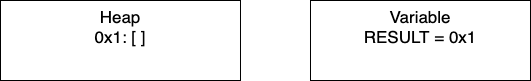
I = 1: Now we have entered the loop and on line 4, we add more characters to our array. At this point, we would have only entry 0x1 in our heap and our variable RESULT would have the pointer 0x1. Continuing through the code, line 5 determines if I is divisible by 2. In this iteration I = 1, so we take the else branch. We again add characters to our array. In total, we have written 5 characters. We then increment I and move to the next iteration.
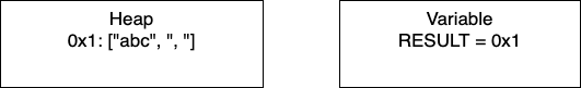
I = 2: We continue the loop and on line 4, we add more characters to our array. We still have just one entry in memory and our pointer is still 0x1. In this iteration, we have written 4 characters. We then increment I and move to the next iteration of the loop.
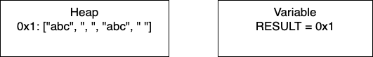
I = 3: We continue the loop and on line 4, we add more characters to our array. In this iteration, we have written 5 characters. We then increment I and thus I = 4 breaking out of the loop.
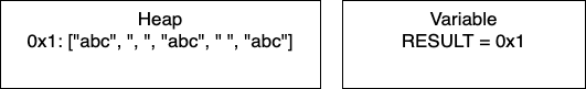
Post-Loop: Once the loop breaks, we join the array to create the final string. This creates a new place in memory and changes RESULT to contain the pointer 0x2.
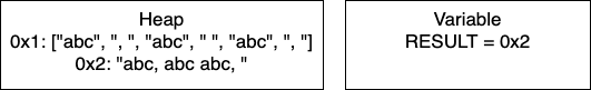
We can do some further analysis of the memory that is required for this particular block.
| Iteration | Memory Entries | Character Copies |
|---|---|---|
| 1 | 2 | 8 |
| 2 | 2 | 17 |
| 3 | 2 | 26 |
| 4 | 2 | 35 |
| . | . | . |
| n | 2 | 9n - 1 |
Again, you need not worry about creating these equations for this course. To illustrate the improvement even more explicitly, let’s consider our previous example with 100K iterations. For APPENDER there were (2x100,000 - 1) = 200,001 memory entries and (9x100,0002 + 7x100,000)/2 = 45 billion character copies. For APPENDER_LIST we now have just 2 memory entries and (9x100,000 - 1) = 899,999 character copies. This dramatic improvement was a result of changing our data structure ever so slightly.
Reference: http://people.cs.ksu.edu/~rhowell/DataStructures/strings/stringbuilders.html
In this module, we reviewed each of the data structures we have explored in this class. Most importantly, we looked at how they compare in terms of performance and discussed some of the best and most efficient ways to use them in our programs.
Using that information, we introduced the standard collection libraries for both Java and Python, and saw how those professional implementations closely follow the same ideas and analysis that we saw in our own structures. While the professional structures may have many more features and more complex code, at the core they still work just like the structures we learned how to build from scratch.
One of the best traits of a good programmer is knowing how to most effectively use the tools made available to us through the programming languages and libraries we have chosen to use. The goal of this class is to give us the background we need to understand how the various collection data structures we can choose from work, so that we can use them in the most effective way to build useful and efficient programs.
YouTube VideoTo start this course, we have looked into strings. They are a very natural way to represent data, especially in real world applications. Often though, the datapoints can be very large and require multiple modifications. We also examined how strings work: element access, retrieving the size, and modifying them. We looked into some alternatives which included StringBuilders for Java and character arrays for Python.
To really understand this point, we have included a comparison. We have implemented the APPENDER and APPENDER_LIST functions in both Python and Java. For the Java implementation, we utilized StringBuilders.
1. function APPENDER(NUMBER, BASE)
2.     RESULT = ""
3.     loop I from 1 to NUMBER
4.         RESULT = RESULT + BASE
5.         if I MOD 2 = 0
6.             RESULT = RESULT + " "
7.         else
8.             RESULT = RESULT + ", "
9.     end loop
10.    return RESULT
11. end function
1. function APPENDER_LIST(NUMBER, BASE)
2. RESULT = []
3. loop I from 1 to NUMBER
4. RESULT.APPEND(BASE)
5. if I MOD 2 = 0
6. RESULT.APPEND(" ")
7. else
8. RESULT.APPEND(", ")
9. end loop
10. RESULT = "".JOIN(RESULT)
11. return RESULT
12. end functionFor the tests of 108 and 109 in Java, the string implementation took over 24 hours and the StringBuilder implementation ran out of memory. For these reasons, they are omitted from the figure.
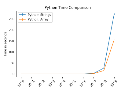
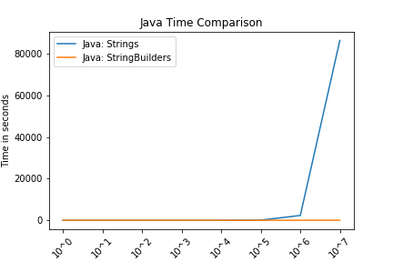
These figures compare Strings and lists for Python and Strings and StringBuilders for Java. The intention of these is not to compare Python and Java.
In both languages, we see that the string function and the respective alternative performed comparably until approximately 106 (1,000,000 characters). Again, these are somewhat contrived examples with the intention of understanding side effects of using strings.
As we have discussed, modern coding languages will have clean up protocols and memory management strategies. With the intention of this class in mind, we will not discuss the memory analysis in practice.
When modifying strings we need to be cognizant of how often we will be making changes and how large those changes will be. If we are just accessing particular elements or only doing a few modifications then using plain strings is a reasonable solution. However, if we are looking to build our own DNA sequence this is not a good way to go as strings are immutable.
All about trees!
For the next data structure in the course, we will cover trees, which are used to show hierarchical data. Trees can have many shapes and sizes and there is a wide variety of data that can be organized using them. Real world data that is appropriate for trees can include: family trees, management structures, file systems, biological classifications, anatomical structures and much more.
We can look at an example of a tree and the relationships they can show. Consider this file tree; it has folders and files in folders.
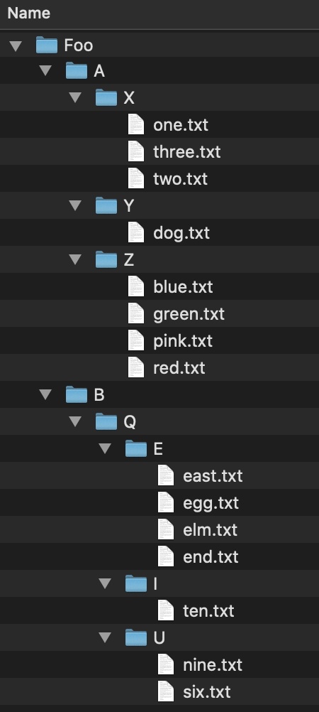
If we wanted to access the file elm.txt, we would have to follow this file path: Foo/B/Q/E/elm.txt. We can similarly store the file structure as a tree like we below. As before, if we wanted to get to the file elm.txt we would navigate the tree in the order: Foo -> B -> Q -> E -> elm.txt. As mentioned before, trees can be used on very diverse data sets; they are not limited to file trees!

In the last module we talked about strings which are a linear data structure. To be explicit, this means that the elements in a string form a line of characters. A tree, by contrast, is a hierarchal structure which is utilized best in multidimensional data. Going back to our file tree example, folders are not limited to just one file, there can be multiple files contained in a single folder- thus making it multidimensional.
Consider the string “abc123”; this is a linear piece of data where there is exactly one character after another. We can use trees to show linear data as well.

While trees can be used for linear data, it would be excessive and inefficient to implement them for single strings. In an upcoming module, we will see how we can use trees to represent any number of strings! For example, this tree below contains 7 words: ‘a’, ‘an’, ‘and’, ‘ant’, ‘any’, ‘all’, and ‘alp’.

In the next sections, we will discuss the properties of a tree data structure and how we would design one ourselves. Once we have a good understanding of trees and the properties of trees, we will implement our own.
The video incorrectly states the degree of a tree is equal to the degree of the root. The correct definition is that the degree of a tree is the largest degree of any node in the tree.
To get ourselves comfortable in working with trees, we will outline some standard vocabulary. Throughout this section, we will use the following tree as a guiding example for visualizing the definitions.

Node - the general term for a structure which contains an item, such as a character or even another data structure.Edge - the connection between two nodes. In a tree, the edge will be pointing in a downward direction.
This tree has five edges and six nodes. There is no limit to the number of nodes in a tree. The only stipulation is that the tree is fully connected. This means that there cannot be disjoint portions of the tree. We will look at examples in the next section.
A rule of thumb for discerning trees is this: if you imagine holding the tree up by the root and gravity took effect, then all edges must be pointing downward. If an edge is pointing upward, we will have a cycle within our structure so it will not be a tree.
Root - the topmost node of the tree
To be a tree, there must be exactly one root. Having multiple roots, will result in a cycle or a tree that is not fully connected. In short, a cycle is a loop in the tree.
Parent - a node with an edge that connects to another node further from the root. We can also define the root of a tree with respect to this definition; Root: a node with no parent.Child - a node with an edge that connects to another node closer to the root.

 In a tree, child nodes must have exactly one parent node. If a child node has more than one parent, then a
 cycle will occur. If there is a node without a parent node, then this is necessarily the root node. There is no limit to the number of child nodes a parent node can have, but to be a parent node, the node must have at least one child node.Leaf - a node with no children.
 This tree has four leaves. There is no limit to how many leaves can be in a tree.
Degree
Degree of a node - the number of children a node has. The degree of a leaf is zero.Degree of a tree - the degree of an entire tree is the largest degree of any node found in the tree.

The degree of the nodes are shown as the values on the nodes in this example. The degree of the tree is the largest degree of any node in the tree. Thus, the degree for this tree is 3.
tree is defined recursively. This means that each child of the root is the root of another tree and the children of those are roots to trees as well. Again, this is a recursive definition so it will continue to the leaves. The leaves are also trees with just a single node as the root.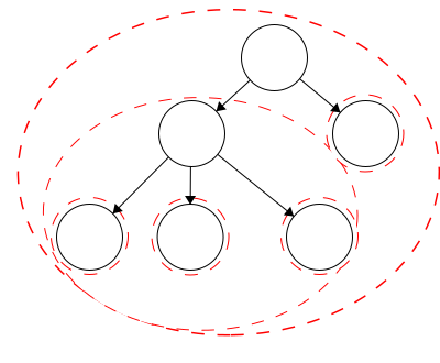 In our example tree, we have six trees. Each tree is outlined in a red dashed circle:
Trees can come in many shapes and sizes. There are, however some constraints to making a valid tree.
Any combination of the following represents a valid tree:
A tree with a single node; just a root,

A tree where each node has a single child, or

A tree where nodes have many children.

Below are some examples of invalid trees.
A cycle
 Again, cycles are essentially loops that occur in our tree. In this example, we see that our leaf has two parents. One way to determine whether your data structure has a cycle is if there is more than one way to get from the root to any node.
A cycle
 Here we can see another cycle. In this case, the node immediately after the root has two parents, which is a clue that a cycle exists. Another test
Two Roots
 Trees must have a single root. In this instance, it may look like we have a tree with two roots. Working through this, we also see that the node in the center has two parents.
Two Trees
 This example would be considered two trees, not a tree with two parts. In this figure, we have two fully connected components. Since they are not connected to each other, this is not a single tree.
Along with understanding how trees work, we want to also be able to implement a tree of our own. We will now outline key components of a tree class.
Recall that trees are defined recursively so we can build them from the leaves up where each leaf is a tree itself. Each tree will have three properties: the item it contains as an object, its parent node of type MyTree, and its children as a list of MyTrees. Upon instantiation of a new MyTree, we will set the item value and initialize the parent node to None and the children to an empty list of type MyTree.
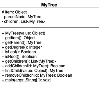
Suppose that we wanted to construct the following tree.

We would start by initializing each node as a tree with no parent, no children, and the item in this instance would be the characters. Then we build it up level by level by add the appropriate children to the respective parent.
Disclaimer: This implementation will not prevent all cycles. In the next module, we will introduce steps to prevent cycles and maintain true tree structures.
In this method, we will take a value as input and then check if that value is the item of a child of the current node. If the value is not the item for any of the node’s children then we should return none.
function FINDCHILD(VALUE)
    FOR CHILD in CHILDREN
        IF CHILD's ITEM is VALUE
            return  CHILD
    return NONE
end functionEach of these will be rather straight forward; children, item, and parent are all attributes of our node, so we can have a getter function that returns the respective values. The slightly more involved task will be getting the degree. Recall that the degree of a node is equal to the number of children. Thus, we can simply count the number of children and return this number for the degree.
We will have two functions to check the node type: one to determine if the node is a leaf and one to determine if it is a root. The definition of a leaf is a node that has no children. Thus, to check if a node is a leaf, we can simply check if the number of children is equal to zero. Similarly, since the definition of a root is a node with no parent, we can check that the parent attribute of the node is None.
When we wish to add a child, we must fisrt make sure we are able to add the child.
MyTreeWe will return true if the child was successfully added and false otherwise while raising the appropriate errors.
function ADDCHILD(CHILD)
    IF CHILD has PARENT
        throw exception
    IF CHILD is CHILD of PARENT
        return FALSE
    ELSE
        append CHILD to PARENT's children
        set CHILD's parent to PARENT
        return TRUE
end function
As an example, lets walk through the process of building the tree above:
a with item ‘A’b with item ‘B’c with item ‘C’d with item ‘D’e with item ‘E’f with item ‘F’g with item ‘G’h with item ‘H’i with item ‘I’g to tree dh to tree di to tree de to tree bf to tree bOnce we have completed that, visually, we would have the tree above and in code we would have:
a with parent_node = None, item = ‘A’, children = {b,c,d}b with parent_node = a, item = ‘B’, children = {e,f}c with parent_node = a, item = ‘C’, children = { }d with parent_node = a, item = ‘D’, children = {g,h,i}e with parent_node = b, item = ‘E’, children = { }f with parent_node = b, item = ‘F’, children = { }g with parent_node = d, item = ‘G’, children = { }h with parent_node = d, item = ‘H’, children = { }i with parent_node = d, item = ‘I’, children = { }Note: When adding a child we must currently be at the node we want to be the parent. Much like when you want to add a file to a folder, you must specify exactly where you want it. If you don’t, this could result in a wayward child.
In the case of removing a child, we first need to check that the child we are attempting to remove is an instance of MyTree. We will return true if we successfully remove the child and false otherwise.
function REMOVECHILD(CHILD)
    IF CHILD in PARENT'S children
        REMOVE CHILD from PARENT's children
        SET CHILD's PARENT to NONE
        return TRUE
    ELSE
        return FALSE
end function
As with adding a child, we need to ensure that we are in the ‘right place’ when attempting to remove a child. When removing a child, we are not ’erasing’ it, we are just cutting the tie from parent to child and child to parent. Consider removing d from a. Visually, we would have two disjoint trees, shown below:

In code, we would have:
a with parent_node = None, item = ‘A’, children = {b,c}b with parent_node = a, item = ‘B’, children = {e,f}c with parent_node = a, item = ‘C’, children = { }d with parent_node = None, item = ‘D’, children = {g,h,i}e with parent_node = b, item = ‘E’, children = { }f with parent_node = b, item = ‘F’, children = { }g with parent_node = d, item = ‘G’, children = { }h with parent_node = d, item = ‘H’, children = { }i with parent_node = d, item = ‘I’, children = { }Many of the terms used in trees relate to terms used in family trees. Having this in mind can help us to better understand some of the terminology involved with abstract trees. Here we have a sample family tree.

Ancestor - The ancestors of a node are those reached from child to parent relationships. We can think of this as our parents and our parent’s parents, and so on.
Descendant - The descendants of a node are those reached from parent to child relationships. We can think of this as our children and our children’s children and so on.
Siblings - Nodes which share the same parent
We can describe the sizes of trees and position of nodes using different terminology, like level, depth, and height.
Level - The level of a node characterizes the distance between the node and the root. The root of the tree is considered level 1. As you move away from the tree, the level increases by one.
Depth - The depth of a node is its distance to the root. Thus, the root has depth zero. Level and depth are related in that: level = 1 + depth.
Height of a Node - The height of a node is the longest path to a leaf descendant. The height of a leaf is zero.
Height of a Tree - The height of a tree is equal to the height of the root.
When working with multidimensional data structures, we also need to consider how they would be stored in a linear manner. Remember, pieces of data in computers are linear sequences of binary digits. As a result, we need a standard way of storing trees as a linear structure.

Path - a path is a sequence of nodes and edges, which connect a node with its descendant. We can look at some paths in the tree above:
Q to O: QRO
Traversal is a general term we use to describe going through a tree. The following traversals are defined recursively.
Pre refers to the root, meaning the root goes before the children.QWYUERIOPTA
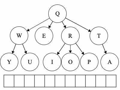
Post refers to the root, meaning the root goes after the children.YUWEIOPRATQ

When we talk about traversals for general trees we have used the phrase ’the traversal could result in’. We would like to expand on why ‘could’ is used here. Each of these general trees are the same but their traversals could be different. The key concept in this is that for a general tree, the children are an unordered set of nodes; they do not have a defined or fixed order. The relationships that are fixed are the parent/child relationships.


| Tree | Preorder | Postorder |
|---|---|---|
| Tree 1 | QWYUERIOPTA |
YUWEIOPRATQ |
| Tree 2 | QETARIOPWUY |
EATIOPRUYWQ |
| Tree 3 | QROPITAEWUY |
OPIRATEUYWQ |

A binary tree is a type of tree with some special conditions. First, it must follow the guidelines of being a tree:
The special conditions that we impose on binary trees are the following:
To reinforce these concepts, we will look at examples of binary trees and examples that are not binary trees.

This is a valid binary tree. We have a single node, the root, with no children. As with general trees, binary trees are built recursively. Thus, each node and its child(ren) are trees themselves.

This is also a valid binary tree. All of the left children are less than their parent. The node with item ‘10’ is also in the correct position as it is less than 12, 13, and 14 but greater than 9.

We have the same nodes but our root is now 12 whereas before it was 14. This is also a valid binary tree.

Here we have an example of a binary tree with alphabetical items. As long as we have items which have a predefined order, we can organize them using a binary tree.

We may be inclined to say that this is a binary tree: each node has 0, 1, or 2 children and amongst children and parent nodes, the left child is smaller than the parent and the right child is greater than the parent. However, in binary trees, all of the nodes in the left tree must be smaller than the root and all of the nodes in the right tree must be larger than the root. In this tree, D is out of place. Node D is less than node T but it is also less than node Q. Thus, node D must be on the right of node Q.

In this case, we do not have a binary tree. This does fit all of the criteria for being a tree but not the criteria for a binary tree. Nodes in binary trees can have at most 2 children. Node 30 has three children.
In the first module we discussed two types of traversals: preorder and postorder. Within that discussion, we noted that for general trees, the preorder and postorder traversal may not be unique. This was due to the fact that children nodes are an unordered set.
We are now working with binary trees which have a defined child order. As a result, the preorder and postorder traversals will be unique! These means that for a binary tree when we do a preorder traversal there is exactly one string that is possible. The same applies for postorder traversals as well.
Recall that these were defined as such:
Now for binary trees, we can modify their definitions to be more explicit:
Let’s practice traversals on the following binary tree.


Since we have fixed order on the children, we can introduce another type of traversal: in-order traversal.
In-order Traversal:
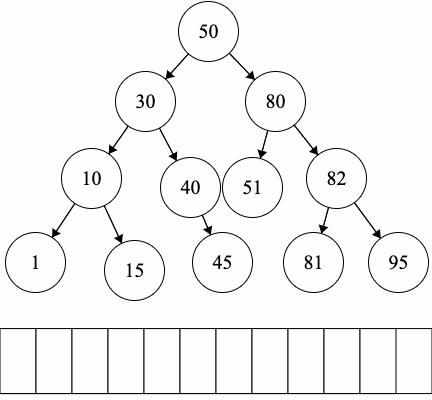
While this is a valid binary tree, it is not balanced. Let’s look at the following tree.
We have the same nodes but our root is now 12 whereas before it was 14. This is a valid binary tree. We call this a balanced binary tree. A balanced binary tree looks visually even amongst the left and right trees in terms of number of nodes.
Note: Balancing is not necessary for a valid binary tree. It is, however, important in terms of time efficiency to have a balanced tree. For example, the number of actions when inserting an element is about the same as the number of levels in the tree. If we tried to add the value 11 into the unbalanced tree, we would traverse 5 nodes. If we tried to add the value 11 in to the balanced tree, we would traverse just 3 nodes.
We believe that balancing binary trees is out of the scope of this course. If you are interested in how we might balance a tree, feel free to check out these videos by Dr. Joshua Weese.
YouTube Video YouTube VideoIn this module we have introduce vocabulary related to trees and what makes a tree a tree. To recap, we have introduced the following:
Child - a node with an edge that connects to another node closer to the root.Degree
Degree of a node - the number of children a node has. The degree of a leaf is zero.Degree of a tree - the degree of an entire tree is the largest degree of any node found in the tree.Edge - connection between two nodes. In a tree, the edge will be pointing in a downward direction.Leaf - a node with no children.Node - the general term for a structure which contains an item, such as a character or even another data structure.Parent - a node with an edge that connects to another node further from the root. We can also define the root of a tree with respect to this definition;Root - the topmost node of the tree; a node with no parent.Now we will work on creating our own implementation of a tree. These definitions will serve as a resource to us when we need refreshing on meanings; feel free to refer back to them as needed.
We discussed more terminology related to trees as well as tree traversals. To recap the new vocabulary:
Ancestor - The ancestors of a node are those reached from child to parent relationships. We can think of this as our parents and the parents of our parents, and so on.Depth - The depth of a node is its distance to the root. Thus, the root has depth zero. Level and depth are related in that: level = 1 + depth.Descendant - The descendants of a node are those reached from parent to child relationships. We can think of this as our children and our children’s children and so on.Height of a Node - The height of a node is the longest path to a leaf descendant. The height of a leaf is zero.Height of a Tree - The height of a tree is equal to the height of the root.Level - The level of a node characterizes the distance the node is from the root. The root of the tree is considered level 1. As you move away from the tree, the level increases by one.Path - a sequence of nodes and edges which connect a node with its descendant.Siblings - Nodes which share the same parentTraversal is a general term we use to describe going through a tree. The following traversals are defined recursively.
Representing data in a graph!
The next data structure we will introduce is a graph.

Graphs are multidimensional data structures that can represent many different types of data. We can use graphs to represent electronic circuits and wiring, transportation routes, and networks such as the Internet or social groups.
A popular and fun use of graphs is to build connections between people such as Facebook friends or even connections between performers. One example is the parlor game Six Degrees of Kevin Bacon. Players attempt to connect Kevin Bacon to other performers through movie roles in six people or less.

For example, Laurence Fishburne and Kevin Bacon are directly connected via ‘Mystic River’. Keanu Reeves and Kevin Bacon have never performed in the same film, but Keanu Reeves and Laurence Fishburne are connected via ‘The Matrix’. Thus, Keanu and Kevin are connected via Laurence.
In this module we will discuss graphs in more detail and build our own implementation of graphs.
We will discuss some of the basic terminology associated with graphs. Some of this vocabulary should feel familiar from the trees section; trees are a specific type of graph!
Nodes: Node is the general term for a structure which contains an item.
Size: The size of a graph is the number of nodes.Capacity: The capacity of a graph is the maximum number of nodes.Nodes can be, but are not limited to the following examples: - physical locations (IE Manhattan, Topeka, Salina), - computer components (IE CPU, GPU, RAM), or - people (IE Kevin Bacon, Laurence Fishburne, Emma Stone)
Edges: Edges are the connection between two nodes. Depending on the data, edges can represent physical distance, films, cost, and much more.
Adjacent: Node A and node B are said to be adjacent if there is an edge from node A to node B.Neighbors: The neighbors of a node are nodes which are adjacent to the node.Edges can be, but are not limited to: - physical distances, like the distance between cities or wiring between computer components, - cost, like bus fares, and - films, like the Six Degrees of Kevin Bacon example
Cycles: A cycle is a path where the first and last node are the only repeated nodes. More explicitly, this means that we start at node A and are able to end up back at node A.For example, we can translate the Amtrak Train Station Connections into a graph where the edges represent direct train station connections.
Within this context, we could say that Little Rock and Fort Worth are adjacent. The neighbors of San Antonio are Fort Worth, Los Angeles, and New Orleans. The Amtrak Train Graph has multiple cycles. One of these is Kansas City -> St. Louis -> Chicago -> Kansas City.
Generated using the Amtrak system map from 2018. This graph does not include all stations or connections. ↩︎
While trees are a type of graph, graphs can have more functionality than trees. For example, recall that to be a single tree, there could be no disconnected pieces.
Connectedness: Graphs do not require being fully connected. There can be disconnected portions within a graph. For example, the following graph shows all of the students in a sophomore biology class. There is an edge between two student nodes if they are Facebook friends.
Graphs can also have loops. In a tree, this would be like a node being its own parent, which is not an allowable condition.
Loops: Loops are edges which connect a node to itself. These can be useful in depicting graphs that show control flow in programming. In this example, node A is connected to node B and node A is connected to itself.
A weighted graph is a graph which has weights associated with the edges. These weights quantify the relationships, so they can represent dollars, minutes, miles, and many other factors which our data may depend upon.
Weights are not limited to physical quantities; they can also be our own defined similarity in text, product types, and anything for which we can create a similarity measure for. Let’s look at concrete weights using the Amtrak example.
We are able to expand the Amtrak graph from the previous page to include approximate distances in miles between cities.
Now that we have weights defined on our edges, we can compare paths in a different way. When we discussed trees, we just looked at the number of edges it took to get to another node. We can also determine the shortest path between nodes with respect to distance. If we wanted to travel from San Antonio to Kansas City, we may be tempted to travel San Antonio -> Los Angeles -> Albuquerque -> Kansas City as it has the fewest stops. This trip would take us 2,531 miles (1201+640+690). With the edge weights in mind, a much better route would be San Antonio -> Fort Worth -> Little Rock -> St. Louis -> Kansas City with a total of 1,089 miles(238+320+293+238) traveled.
Generated using the Amtrak system map from 2018. This graph does not include all stations or connections. Distance was calculated approximately ‘as the crow flies’. ↩︎
A directed graph is a graph that has a direction associated with each edge. For example, trees are a directed graph. The edge orientation will imply a fixed direction that we can move about nodes. As with trees, the flat end of the arrow will represent the origin and the arrowhead will represent the destination. If an edge has no arrowheads, then it is assumed that we can traverse both directions.
In the following graph, we have an example distribution network where each store ends up with 5 units in its possession. For example, nine units go from the distribution center to Store A. The distribution center will never receive product from stores as it has no incoming edges.

Unlike trees, directed graphs can have nodes with multiple incoming edges. We can see an example of this at Store B. The distribution center and Store A both send units to Store B.
In directed graphs, we must be cautious on how we define adjacent. For the following, we would say that the source is adjacent to the target. However, the target is not adjacent to the source.

Formally, node A and node B are said to be adjacent if there is an edge from node A to node B.
When discussing directed graphs, we must also talk about undirected graphs. An undirected graph is a graph in which none of the edges have an orientation. If there is at least one directed edge, then it is considered a directed graph.
Undirected Edge: An undirected edge is an edge which has no defined orientation (IE no arrowheads) which implies that we can traverse in either direction. If node A and node B are connected via an undirected edge then we say node A is adjacent to node B and node B is adjacent to node A.For the following undirected edge, we would say that the source is adjacent to the target and the target is adjacent to the source.

Graph types and appearances can vary wildly. We are not limited to just weighted/unweighted or directed/undirected. We can also have combinations of weighted and directed.
In the following graph, we have an example of a weighted and directed map. This map represents a zoo train where each node represents a station and each edge is a part of the track. Zoo guests can get on and off wherever they desire.
This graph is weighted as guests must pay the associated fee for each part of the track. Our example train also has a one way direction in most cases. The exception to this is the entrance/exit to the aquarium, this part of the track can go either direction.
In this graph, we also have a couple of loops. This would allow for zoo-guests to ride the train around an expansive exhibit such as the elephants or giraffes.
One possible way to tour the zoo for a guest starting at the entrance could be: aquarium, primates, big cats, antelope, giraffes, loop around the giraffes, elephants, aquarium, then exit. Their total payment for just the train would be $14.

The first way that we can represent graphs is as matrices. In a matrix representation of a graph, we will have an array with all the nodes and a matrix to depict the edges. The matrix that depicts the edges is called the adjacency matrix.
To build the adjacency matrix, we go through the nodes and edges. If there is an edge with weight w going from i to j, then we put w in the (i,j) spot in our adjacency matrix. If there is no edge from i to j then we put infinity in the spot (i,j). Let’s look at some examples.
An edge that starts at source and ends at target will result in an entry at (source,target) in the adjacency matrix.
For an unweighted graph, we treat the weights as 1 for all edges in our adjacency matrix.
For an undirected edge between nodes i and j, we put an edge from i to j and an edge from j to i.
Suppose that we have the following graph:

Across the top of the following, we have the array of nodes. This give us the index at which each node is located. For example, node A is in spot 1, node B is in spot 2, node C is in spot 3 and so on.
Below that we have the adjacency matrix. For the directed edge with weight 2 that goes from node B to node C, we have the value 2 at (2,3) in the adjacency matrix as B has index 2 and C has index 3. For the directed edge with weight 4 that goes from node A to node F, we have the value 4 at (1,6) in the adjacency matrix as A has index 1 and F has index 6.
Since there is no edge that connects from node A to node B, we have infinity in (1,2).

Now suppose we have this graph. We now have some loops present.

For example, we have a loop on node E with weight 12 so we will put the value 12 in spot (5,5) as E has index 5.

Now suppose we have this graph which is undirected and unweighted.

Since this graph is unweighted, we will treat all edges as though they have weight equal to one. Since this graph is undirected, each edge will essentially show up twice.
For example, for the edge that connects nodes A and B, we will have an entry in our adjacency matrix at (1,2) and (2,1).

In the previous module, we introduced graphs and a matrix-based implementation. For this module, we will continue working with graphs and change our implementation to lists.
When using graphs, a lot of situational variation can occur. Some graphs can have a few nodes with many edges, many nodes with few edges, and so on. When we use the matrix implementation, we initialize a matrix with the number of columns and rows equal to the number of nodes. For example, if we have a graph with 20 nodes, our adjacency matrix would have 20 rows and 20 columns, resulting in 400 potential entries.
First let’s look at the implementation and then we will discuss when one may be better than the other.
In the matrix representation, we had an array of the node items. In the list representation, we will have an array of node objects. Each node object will keep track of the node item, the node index, and the outgoing edges.

The item can be any object and the index will be a value within our capacity. The edges will be a list of pairs where the first entry is the index of the target node and the second entry is the weight of the edge.
Since each node will track its neighbors, it is important that we are consistent in our indexing of nodes. If our nodes were to get out of order, then our edges would as well.
Consider the following graph which we saw in the matrix representation.
The following list of nodes depicts the graph above. We can see that each node object has the item and index.
If we look closer at the edges of the node with item A and index 1, we see that the set of edges is equal to [(4, 3.0), (6, 4.0)]. This corresponds to the fact that there are two edges with the source as node 1. The first ordered pair, (4, 3.0), means that there is an edge with source node 1 (A) and target node 4 (D) that has weight 3. We can confirm that in our graph we do have an edge from A to D with weight 3.

The following includes a couple of examples of loops within our graph.
We have loops on nodes D, E, and F in our graph. Recall that a loop is an edge where the source and target are the same. For example, we have an edge with source D and target D that has weight 12. We see this in our list representation in the node object with item D and index 4, where we have the entry (4,12.0) in the edges.

When considering which implementation to use, we need to consider the connectivity in our graph. The terms that we use to describe the connectedness are dense and sparse.
Dense Graph: A dense graph is a graph in which there is a large number of edges. Typically in a dense graph, the number of edges is close to the maximum number of edges.Sparse Graph: A sparse graph is a graph in which there is a small number of edges. In this case the number of edges is considerably less than the maximum number of edges.Intuitively, we can think of dense and sparse in terms of populations. For example, if 100 people lived in a city block, we can consider that to be densely populated. If 100 people lived in 100 square miles we can consider that to be sparsely populated.
Let’s look at some motivating examples to get an idea of how the different structures will handle these cases.
The following is a dense graph. In this case, our graph does have the maximum number of edges. This means that every node is connected to every other node including itself.


The following is a sparse graph.


For dense graphs, the matrix representation will have better qualities as we are already setting aside space for the maximum number of edges. Sparse graphs are better represented in the list representation.
When we initialize the matrix implementation, we initialize the nodes attribute to have dimension equal to the capacity of the graph. The edges attribute is initialized to be a square matrix with dimension equal to capacity by capacity. Thus, if we have a sparse matrix, we are representing a lot of non-existent edges.
When we initialize the list implementation, we just have the nodes attribute which has dimension equal to the capacity and each node tracks its own edges. If we have a dense matrix and we are searching for an edge, we must loop through each edge from the target node to see if the edge exists. In the matrix representation, we can access that edge directly.
If the proportion of edges to the maximum number of edges is greater than 1/64, then the matrix representation is better in terms of space.

nodes: This will keep track of the nodes which are in our graph as well as the node values. The nodes can have any type of value such as numbers, characters, and even other data structures.size: This will keep track of the number of nodes that are active in our graph.Upon initialization, we will initialize nodes to be an empty array with dimension capacity and size to be zero as we start with no actual nodes.
get nodes: returns a list of the nodes with their respective indexes. This will be the same logic from our matrix graph.function GETNODES()
LIST = []
for NODE in NODES
if NODE has a VALUE
append (VALUE, INDEX) to LIST
return LISTget edges: returns a list of the edges in the format (source, target, weight).function GETEDGES()
LIST = []
for NODE in NODES
if NODE is not empty
for EDGE in NODE EDGES
TAR = first entry of EDGE
WEIGHT = second entry of EDGE
append (NODE,TAR,WEIGHT) to LIST
return LISTget node: returns the node with the given index. If the index is within the possible range, then we return the value of that node. This will be the same logic from our matrix graph.
find node: returns the index of the given node. We iterate through our nodes and if we find that value, then we return the index. Otherwise, return -1. This will be the same logic from our matrix graph.
get edge: returns the weight of the edge between the given indexes of the source node and target node. If one or both of the indexes are out of range, then we should return infinity. From the source node object, we will call the graph node get edge function on the target index.
function GETEDGE(SRC,TAR)
    if SRC and TAR are between 0 and capacity
        SRCNODE = the node at index SRC of the NODES attribute
        WEIGHT = call the graph node GETEDGE from SRCNODE on TAR
        return WEIGHT
    else
        return infinity
get capacity: returns the maximum number of nodes we are allowed to have. Upon initialization, we will have a fixed number of possible nodes in our node array. We can simply return the size of this array. This will be the same logic from our matrix graph.
get size: returns the size attribute. This will be the same logic from our matrix graph.
get number of edges: returns the number of edges currently in the graph.
function NUMBEROFEDGES()
    COUNT = 0
    for NODE in NODES
        if NODE is not empty
            for EDGE in NODE EDGES
                increment COUNT by one
    return COUNT
get neighbors: returns the neighbors of the given node. We will access our row adjacency matrix that corresponds to the node and return the indexes and values of those entries which are not infinity.function GETNEIGHBORS(IDX)
SRCNODE = the node at index IDX of the NODES attribute
if SRCNODE is not empty
return SRCNODE's edges
else
return nothing
In this module, we have introduced the graph data structure. We also looked at how we would implement a graph using a matrix representation. We introduced the following new concepts in this module:
Directed Graphs: A directed graph is a graph that has a direction associated with each edge. The flat end of the arrow will represent the origin and the arrowhead will represent the destination. If an edge has no arrowheads, then it is assumed that we can traverse both directions.
Edges: Edges are the connection between two nodes. Depending on the data, edges can represent physical distance, films, cost, and much more.
Adjacent: Node A and node B are said to be adjacent if there is an edge from node A to node B.Neighbors: The neighbors of a node are nodes which are adjacent to the node.Undirected Edge: An undirected edge is an edge which has no defined orientation (IE no arrowheads). If node A and node B are connected via an undirected edge then we say node A is adjacent to node B and node B is adjacent to node A.Loops: Loops are edges which connect a node to itself.
Nodes: Node is the general term for a structure which contains an item.
Size: The size of a graph is the number of nodes.Capacity: The capacity of a graph is the maximum number of nodes.Weighted Graphs: A weighted graph is a graph which has weights associated with the edges. These weights will quantify the relationships so they can represent dollars, minutes, miles, and many other factors which our data may depend on.
Graphs can be represented using a matrix of edges between nodes.
In this module, we also introduced a new way to store the graph data structure. Thus, we now have two ways to work with graphs, in lists and in matrices:
While these methods show the same information, there are cases when one way may be more desirable than the other.
We discussed how a sparse graph is better suited for a list representation and a dense graph is better suited for a matrix representation. We also touched on how working with the edges in a list representation can add complexity to our edge functions. If we are needing to access edge weights or update edges frequently, a matrix representation would be a good choice – especially if we have a lot of nodes.
Algorithms for working with graphs!
In the previous modules, we have introduced graphs and two implementations. This module will cover the traversals through graphs as well as path search techniques.
As we have discussed previously, graphs can have many applications. Based on that, there are many things that we may want to infer from graphs. For example, if we have a graph that depicts a railroad or electrical network, we could determine what maximum flow of the network. The standard approach for this task is the Ford-Fulkerson Algorithm. In short, given a graph with edge weights that represent capacities the algorithm will determine the maximum flow throughout the graph.
From the matrix graph module, we used the following distribution network as an example.
Conceptually, we would want to determine the maximum number of units that could leave the distribution center without having excess laying around stores. Using the maximum flow algorithm, we would determine that the maximum number of units would be 15.

The driving force in the Ford-Fulkerson algorithm, as well as other maximum flow algorithms, is the ability to find a path from a source to a target. Specifically, these algorithms use breadth first and depth first searches to discover possible paths.
To get to introducing the searches, we will first discuss the basis of them. Those are the depth first traversal and the breadth first traversal. We will outline the premise of these traversals and then discuss how we can modify their algorithms for various tasks, such as path searches.
We can perform these traversals on any type of graph. Conceptually, it will help to have a tree-like structure in mind to differentiate between depth first and breadth first.

First we will discuss Depth First Traversal. We can define the depth first traversal in two ways, iteratively or recursively. For this course, we will define it iteratively.
In the iterative algorithm, we will initialize an empty stack and an empty set. The stack will determine which node we search next and the set will track which nodes we have already searched.
Recall that a stack is a ‘Last In First Out’ (LIFO) structure. Based on this, the depth first traversal will traverse a nodes descendants before its siblings.
To do the traversal, we must pick a starting node; this can be an arbitrary node in our graph. If we were doing the traversal on a tree, we would typically select the root at a starting point. We start a while loop to go through the stack which we will be pushing and popping from. We get the top element of the stack, if the node has not been visited yet then we will add it to the set to note that we have now visited it. Then we get the neighbors of the node and put them onto the stack and continue the process until the stack is empty.
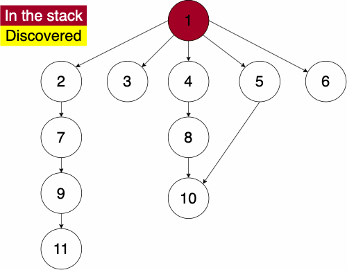
function DEPTHFIRST(GRAPH,SRC)
    STACK = empty array
    DISCOVERED = empty set
    append SRC to STACK
    while STACK is not empty
        CURR = top of the stack
        if CURR not in DISCOVERED
            add CURR to DISCOVERED
            NEIGHS = neighbors of CURR
            for EDGE in NEIGHS
                NODE = first entry in EDGE
                append NODE to STACK
Since the order of the neighbors is not guaranteed, the traversal on the same graph with the same starting node can find nodes in different orders.
We can also perform a breadth first traversal either iteratively or recursively. As with the depth first traversal, we will define it iteratively.
In the iterative algorithm, we initialize an empty queue and an empty set. Like depth first traversal, the set will track which nodes we have discovered. We now use a queue to track which node we will search next.
Recall that a queue is a ‘First In First Out’ (FIFO) structure. Based on this, the breadth first traversal will traverse a nodes siblings before its descendants.
Again, we must pick a starting node; this can be an arbitrary node in our graph. We add the starting node to our queue and the set of discovered nodes. We start a while loop to go through the queue which we will be enqueue and dequeue from. We get the first element of the queue, then get the neighbors of the current node. We loop through each edge adding the neighbor to the discovered set and the queue if it has not already been discovered. We continue this process until the queue is empty.
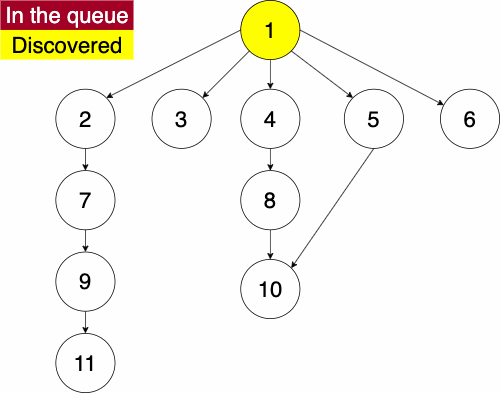
function BREADTHFIRST(GRAPH,SRC)
    QUEUE = empty queue
    DISCOVERED = empty set
    add SRC to DISCOVERED
    add SRC to QUEUE
    while QUEUE is not empty
        CURR = first element in QUEUE
        NEIGHS = neighbors of CURR
        for EDGE in NEIGHS
            NODE = first entry in EDGE
            if NODE is not in DISCOVERED
                add NODE to DISCOVERED
append NODE to QUEUEIt is important to remember in these implementations that a stack is used for depth first and a queue is used for a breadth first. The stack, being a LIFO structure, will proceed with the newest entry which will put us farther away from the source. The queue, being a FIFO structure, will proceed with oldest entry which will focus the algorithm more on the adjacent nodes. If we were to use say a queue for a depth first search, we would be traversing neighbors before descendants.
When introducing graphs, we discussed how the components of a graph didn’t have to all be connected. If our goal is to visit each node, like in the searches, then we will need to perform the search from every node.
For example, the graph below has two separate components. Lets walk through which nodes we will discover by calling the traversals from each node.

| Start | Visited (in alphabetical order) |
|---|---|
| A | {A, D, H} |
| B | {B, E, H, I} |
| C | {C} |
| D | {D} |
| E | {E, H, I} |
| F | {C, F} |
| G | {C, G} |
| H | {H} |
| I | {I} |
| J | {C, F, G, J} |
In this example, we would need to call either traversal on nodes A, B and J in order to visit all of the nodes.
An important application for these traversals is the ability to find a path between two nodes. This has many applications in railroad networks as well as electrical wiring. With some modifications to the traversals, we can determine if electricity can flow from a source to a target. We will modify depth first and breadth first traversals in similar ways.
There are three cases that can happen when we search for a path between nodes:
With these searches, we are not guaranteed to return the same path if there are multiple paths.
We will call these Depth First Search (DFS) and Breadth First Search (BFS). In both traversals, we have added the following extra lines: 4, 9-16, and 22 through the end.
First, we have the addition of PARENT_MAP which will be a dictionary to keep track of how we get from one node to another. We will use the convention of having the key be the child and the value be the parent. While we use the terms child and parent, this is not exclusive to trees.
The ending portion starting at line 22, will add entries to our dictionary. If we haven’t already found an edge to NODE, then we will add the edge that we are currently on.
The other addition is the block of code from line 9 to 16. We will enter this if block if the node that we are currently at is the target. This means that we have finally found a path from the source node to the target node. The process in this segment of code will backtrack through the path and build the path.
 1function DEPTHFIRSTSEARCH(GRAPH,SRC,TAR)
 2    STACK = empty array
 3    DISCOVERED = empty set
 4    PARENT_MAP = empty dictionary
 5    append SRC to STACK
 6    while STACK is not empty
 7        CURR = top of the stack
 8        if CURR not in DISCOVERED
 9            if CURR is TAR
10                 PATH = empty array
11                 TRACE = TAR
12                 while TRACE is not SRC
13                     append TRACE to PATH
14                     set TRACE equal to PARENT_MAP[TRACE]
15                 reverse the order of PATH
16                 return PATH
17            add CURR to DISCOVERED
18            NEIGHS = neighbors of CURR
19            for EDGE in NEIGHS
20                NODE = first entry in EDGE
21                append NODE to STACK
22                if PARENT_MAP does not have key NODE
23                    in the PARENT_MAP dictionary set key NODE with value CURR
24    return nothing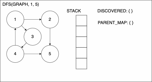
 1function BREADTHFIRSTSEARCH(GRAPH,SRC,TAR)
 2    QUEUE = empty queue
 3    DISCOVERED = empty set
 4    PARENT_MAP = empty dictionary
 5    add SRC to DISCOVERED
 6    add SRC to QUEUE
 7    while QUEUE is not empty
 8        CURR = first element in QUEUE
 9        if CURR is TAR
10            PATH = empty list
11            TRACE = TAR
12            while TRACE is not SRC
13                    append TRACE to PATH
14                    set TRACE equal to PARENT_MAP[TRACE]
15                reverse the order of PATH
16                return PATH
17        NEIGHS = neighbors of CURR
18        for EDGE in NEIGHS
19            NODE = first entry in EDGE
20            if NODE is not in DISCOVERED
21                add NODE to DISCOVERED
22                if PARENT_MAP does not have key NODE
23                    in the PARENT_MAP dictionary set key NODE with value CURR
24                append NODE to QUEUE
25    return nothing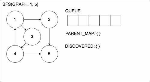
Finding a path in a graph is a very common application in many fields. One application that we benefit from in our day to day lives is traveling. Programs like Google Maps calculate various paths from point A to point B.
In the context of graph data structures, we can think of each intersection as a node and each road as an edge. Google Maps, however, tracks more features of edges than we have discussed. Not only do they track the distance between intersections, they also track time, tolls, construction, road surface and much more. In the next module, we will discuss more details of how we can find the shortest path.
Another application of the general searches is coloring maps. The premise is that we don’t want two adjacent territories to have the coloring. These territories could be states, like in the United States map below, counties, provinces, countries, and much more.
The following was generated for this course using the breadth first search and MyMatrixGraph class that we have implemented in this course. To create the visual rendering, the Python library NetworkX^[https://networkx.github.io/] was used. In this rendering, the starting node was Utah. If we were to start from say Alabama or Florida, we would not have a valid four coloring scheme once we got to Nevada. Since Hawaii and Alaska have no land border with any of the states, they can be any color.

We will continue to work with graph algorithms in this module, specifically with finding minimum spanning trees (MST). MSTs have many real world applications such as:
Suppose we were building an apartment complex and wanted to determine the most cost-effective wiring schema. Below, we have the possible construction costs for wiring apartment to apartment. Wiring vertically adjacent apartments is cheaper than wiring horizontally adjacent units and those closest to the power closet have lower costs as well.

To find the best possible solution, we would find the MST. The final wiring schema may look something like the figure below.

Determining a MST can result in lower costs and time used in many applications, especially logistics. To properly define a minimum spanning tree, we will first introduce the concept of a spanning tree.
A spanning tree for a graph is a subset of the graphs edges such that each node is visited once, no cycles are present, and there are no disconnected components.
Let’s look at this graph as an example. We have five nodes and seven edges.

Below, we have valid examples of spanning trees. In each of the examples, we visit each node and there are no cycles. Recall that a cycle is a path in which the starting node and ending node are the same.

To be a spanning tree of a graph, it must:
Further, we can imagine selecting a node in a spanning tree as the root and letting gravity take effect. This gives us a visual motivation as to why they are called spanning trees. In these examples, we have selected node A for the root for each of the spanning trees above.

Below, we have invalid examples of spanning trees. In the left column, the examples are where all of the nodes are not connected in the same component. In the right column, the examples contain cycles. For example in the top right, we have the cycle B->C->D->E->B

Now that we have an understanding of general spanning trees, we will introduce the concept of minimum spanning trees. First let’s introduce the concept of the cost of a tree.
The cost that is associated with a tree, is the sum of its edges weights. Let’s look at this spanning tree which is from the previous page. The cost associated with this spanning tree is: 2+6+10+14=32.

A minimum spanning tree is a spanning tree that has the smallest cost. Recall the graph from the previous page.
Below on the left is a minimum spanning tree for the graph above. On the right is an example of a spanning tree, though it does not have the minimum cost.

In this small example, it is rather straightforward to find the minimum spanning tree. We can use a bit of trial and error to determine if we have the minimum spanning tree or not. However, once the graphs start to get more nodes and more edges it quickly becomes more complicated.

There are two algorithms that we will introduce to give us a methodical way of finding the minimum spanning tree. The first that we will look at is Kruskal’s algorithm and then we will look at Prim’s algorithm.
As graphs get larger, it is important to go about finding the MST in a methodical way. In the mid 1950’s, there was a desire to form an algorithmic approach for solving the ’traveling salesperson’ problem^[We will describe this problem in a future section of this module]. Joseph Kruskal first published this algorithm in 1956 in the Proceedings of the American Mathematical Society1. The algorithms prior to this were, as Kruskal said, “unnecessarily elaborate” thus the need for a more succinct algorithm arose.
In his original work, Kruskal outlined three different yet similar algorithms to finding a minimum spanning tree. The Kruskal Algorithm that we use is as follows:
u and v are connected by the edge and they are not in the same set yet, then join the two sets and add the edge to your set of edges
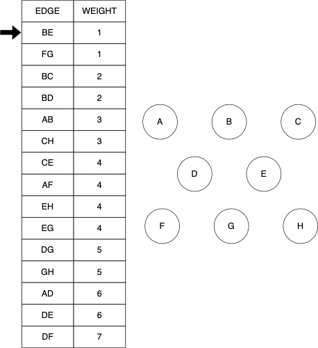

function KRUSKAL(GRAPH)
    MST = GRAPH without the edges attribute(s)
    ALLSETS = an empty list which will contain the sets
    for NODE in GRAPH NODES
        SET = a set with element NODE
        add SET to ALLSETS
    EDGES = list of GRAPH's edges
    SORTEDEDGES = EDGES sorted by edge weight, smallest to largest
    for EDGE in SORTEDEDGES
        SRC = source node of EDGE
        TAR = target node of EDGE
        SRCSET = the set from SETS in which SRC is contained
        TARSET = the set form SETS in which TAR is contained
        if SRCSET not equal TARSET
            UNIONSET = SRCSET union TARSET
            add UNIONSET to ALLSETS
            remove SRCSET from ALLSETS
            remove TARSET from ALLSETS
            add EDGE to MST as undirected edge
return MSTThe history of Prim's Algorithm is not as straight forward as Kruskal’s. While we often call it Prim's Algorithm, it was originally developed in 1930 by Vojtěch Jarník. Robert Prim later rediscovered and republished this algorithm in 1957, one year after Kruskals. To add to the naming confusion, Edsger Dijkstra also published this work again in 1959. Because of this, the algorithm can go by many names: Jarkík's Algorithm, Jarník-Prim's Algorithm, Prim-Dijkstra's Algorithm, and DJP Algorithm.
Prim cited “large-scale communication” as the motivation for this algorithm, specifically the “Bell System leased-line”1. Leased lines were used primarily in a commercial setting which connected business offices that were geographically distant (IE in different cities or even states). Companies would want all offices to be connected but wanted to avoid having to lay an excessive amount of wire. Below is a figure which Prim used to motivate the need for the algorithm. This image depicts the minimum spanning tree which connect each of the US continental state capitals along with Washington D.C.
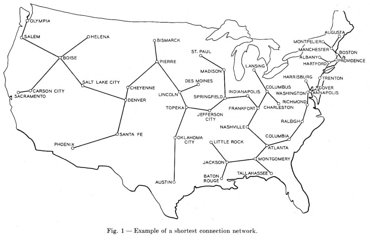
The basis of the algorithm is to start with only the nodes of the graph, then we do the following
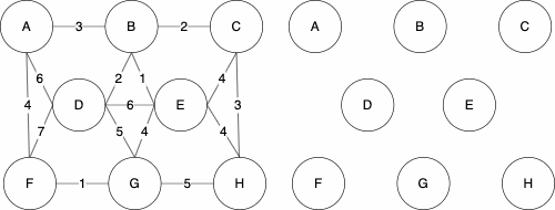

Uniqueness
You may have noticed that the minimum spanning tree that resulted from Kruskal’s algorithm differed from Prim’s algorithm. We have displaying them both below for reference.
| Kruskal | Prim |
|---|---|
|
|
|
While these are different, they are both valid. The trees both have cost 16. The MST of a graph will be unique, meaning there is only one, if none of the edges of the graph have the same weight.
function PRIM(GRAPH, START)
    MST = GRAPH without the edges attribute(s)
    VISITED = empty set
    add START to VISITED
    AVAILEDGES = list of edges where START is the source
    sort AVAILEDGES
    while VISITED is not all of the nodes
        SMLEDGE = smallest edge in AVAILEDGES
        SRC = source of SMLEDGE
        TAR = target of SMLEDGE
        if TAR not in VISITED
            add SMLEDGE to MST as undirected edge
            add TAR to VISITED
            add the edges where TAR is the source to AVAILEDGES
        remove SMLEDGE from AVAILEDGES
        sort AVAILEDGES
    return MST
R.C. Prim, May 8, 1957 Shortest Connection Networks And Some Generalizations https://archive.org/details/bstj36-6-1389 ↩︎
While we won’t outline algorithms suited for solving the traveling salesperson problem (TSP), we will outline the premise of the problem. This problem was first posed in 1832, almost a two centuries ago, and is still quite prevalent. It is applicable to traveling routes, distribution networks, computer architecture and much more. The TSP is a seminal problem that has motivated many research breakthroughs, including Kruskal’s algorithm!
The motivation of the TSP is this: given a set of locations, what is the shortest path such that we can visit each location and end back where started?
Suppose we wanted to take a road trip with friends to every state capital in the continental US as well as Washington D.C. To save money and time, we would want to minimize the distance that we travel. Since we are taking a road trip, we would want to avoid frivolous driving. For example, if we start in Sacremento, CA we would not want to end the trip in Boston, MA. The trip should start and end at the same location for efficiency.
The figure below shows the shortest trip that visits each state capital and Washington D.C. once. In this example, we can start where ever we like and will end up where we started.
In this problem, it is easy to get overwhelmed by all of the possibilities. Since there are 49 cities to visit, there are over 6.2*10^60 possibilities. For reference, 10^12 is equivalent to one trillion! Thus, we need an algorithmic approach to solve this problem as opposed to a brute force method.
A queue that efficiently sorts as data is inserted!
The next data structure we will cover is heaps. The heaps discussed in this course are not to be confused with heaps which refer to garbage collection in certain coding languages. Heaps are good for situations were we will need to frequently access and update the highest (or lowest) priority item in a set. For example, heaps are a good data structure to use in Prim’s algorithm. In Prim’s algorithm, we repeatedly got the smallest edge, removed the smallest edge, and then added to and sorted the list of edges.
A heap is an array which we can view as an unsorted binary tree. This tree must have the following properties:
i of the tree, then level i-1 is full. Below we have an example of how this property has been broken. Level two is not full but there are nodes on level three.


As a consequence of the above properties, the following is true as well: Only one node can have one child, all other nodes will have zero or two children. Try to construct a counterexample to see what we mean!
There are two main types of heaps, the max-heap and the min-heap. Depending on the element we want to access we may use one or the other.
A max-heap is a heap such that the parent node is greater than or equal to the children. For example, if we are using a heap to track work flow,we would want to use a max-heap. In this case, the highest priority element will always be the root of the tree.
A min-heap is a heap such that the parent node is less than or equal to the children. This is the opposite of the max-heap. The root of this heap will be the item with the lowest priority. A min-heap may feel unnatural at first, however, this is ideal for greedy algorithms such as Prim’s algorithm. We are frequently getting the smallest edge.
Heaps can be viewed in two forms: as a tree or as an array. We will use the array style in code but we can have the tree structure in the back of our mind to help understand the order of the data. Here is an example of the heap as a tree on the left and the heap as an array on the right.

The root of the heap will always be the first element. Then we can base the numbering of the following nodes from left to right and top to bottom. For example, the left child of the root will be the second entry and the right child will be the third.
For full functionality of our heap, we want to be able to easily determine the parent of a node as well as the children of a node.
Using just the array, how can we determine the parent of a node? In the example above, how can we determine the parent of the node with value 18?
We can formulate the relationships between parent and children nodes mathematically. For a node at index i, we can say that the left child of i will be at index 2i and the right child will be at 2i+1. Similarly, we can say that the parent of node i will be at index floor(i/2).
The function floor(x) like in floor(i/2) will round decimal values down to the next whole number. Some examples:
floor(3.2)=3floor(1.9999)=1floor(4)=4
| Node | Parent | Left Child | Right Child |
|---|---|---|---|
i |
floor(i/2) |
2i |
2i + 1 |
| 1 | N/A | 2*1=2 |
2*1+1=3 |
| 2 | floor(2/2)=1 |
2*2=4 |
2*2+1=5 |
| 3 | floor(3/2)=1 |
2*3=6 |
2*3+1=7 |
| 4 | floor(4/2)=2 |
2*4=8 |
2*4+1=9 |
| 5 | floor(5/2)=2 |
2*5=10 |
2*5+1=11 |
Consider the following example and try to work some out for yourself.

For example, if we ask for the parent of the node with value 27, our answer would be the node with value 35 The node with value 27 has index 5. Thus, the parent of that node will have index floor(5/2)=2. Node 35 is at index two, as such, node 35 is the parent of node 27.
In a heap where n is the size of heap, the elements floor(n/2)+1 through n will always be leaves. If we assume that we have just the 12 elements in this example, then based on this formula, elements 7 through 12 must be leaves. We can verify this in the tree representation!
A natural implementation of heaps is priority queues.
A priority queue is a data structure which contains elements and each element has an associated key value. The key for an element corresponds to its importance. In real world applications, these can be used for prioritizing work tickets, emails, and much more.

We can use a heap to organize this data for us.

As with heaps, we can have min-priority queues and max-priority queues. For the applications listed above, a max-priority queue is the most intuitive choice. For this course however, we will focus more on min-priority queues which will give us better functionality for greedy algorithms, like Prim’s algorithm.
For the minimum spanning tree algorithms, using a min-priority queue helps the performance of the algorithms. Recall Prim’s algorithm, shown below. Each time we visited a new node, we would add the outgoing edges to the list of available edges, remove the smallest edge, and sort the list.
function PRIM(GRAPH, SRC)
    MST = GRAPH without the edges attribute(s)
    VISITED = empty set
    add SRC to VISITED
    AVAILEDGES = list of edges where SRC is the source
    sort AVAILEDGES
    while VISITED is not all of the nodes
        SMLEDGE = smallest edge in AVAILEDGES
        SRC = source of SMLEDGE
        TAR = target of SMLEDGE
        if TAR not in VISITED
            add SMLEDGE to MST as undirected edge
            add TAR to VISITED
            add the edges where TAR is the source to AVAILEDGES
        remove SMLEDGE from AVAILEDGES
        sort AVAILEDGES
    return MST
If we implement Prim’s algorithm with min-priority queue, we don’t have to worry about sorting the edges every time we add or remove one.
function PRIM(GRAPH, SRC)
    MST = GRAPH without the edges attribute(s)
    VISITED = empty set
    add SRC to VISITED
    AVAILEDGES = min-PQ of edges where SRC is the source
    while VISITED is not all of the nodes
        SMLEDGE = smallest edge in AVAILEDGES
        SRC = source of SMLEDGE
        TAR = target of SMLEDGE
        if TAR not in VISITED
            add SMLEDGE to MST as undirected edge
            add TAR to VISITED
            add the edges where TAR is the source to AVAILEDGES
        remove SMLEDGE from AVAILEDGES
return MSTA good application of priority queues is finding the shortest path in a graph. A common algorithm for this is Dijkstra’s algorithm.
Edsger Dijkstra was a Dutch computer scientist who researched many fields. He is credited for his work in physics, programming, software engineering, and as a systems scientist. His motivation for this algorithm in particular was to be able to find the shortest path between two cities.
What is the shortest way to travel from Rotterdam to Groningen, in general: from given city to given city? It is the algorithm for the shortest path, which I designed in about twenty minutes. One morning I was shopping in Amsterdam with my young fiancée, and tired, we sat down on the café terrace to drink a cup of coffee and I was just thinking about whether I could do this, and I then designed the algorithm for the shortest path. - Edsger Dijkstra, Communications of the ACM 53 (8), 2001.
His original algorithm was defined for a path between two specific cities. Since its publication, modifications have been made to the algorithm to find the shortest path to every node given a source node.
DIJKSTRAS(GRAPH, SRC)
    SIZE = size of GRAPH
    DISTS = array with length equal to SIZE
    PREVIOUS = array with length equal to SIZE
    set all of the entries in PREVIOUS to none
    set all of the entries in DISTS to infinity

    DISTS[SRC] = 0
    PQ = min-priority queue

    loop IDX starting at 0 up to SIZE
        insert (DISTS[IDX],IDX) into PQ

    while PQ is not empty
        MIN = REMOVE-MIN from PQ
        for NODE in neighbors of MIN
            WEIGHT = graph weight between MIN and NODE
            CALC = DISTS[MIN] + WEIGHT
            if CALC < DISTS[NODE]
                DISTS[NODE] = CALC
                PREVIOUS[NODE] = MIN
                PQIDX = index of NODE in PQ
                PQ decrease-key (PQIDX, CALC)
return DISTS and PREVIOUSAside from just finding routes for us to travel, Dijkstra’s algorithm can accommodate for any application that can have an abstraction to finding the shortest path. For example, the following animation shows how a robot could utilize Dijkstra’s algorithm to find the shortest path with an obstacle in the way. In this example, each node could represent one square foot of floor space and the edges would represent those spaces that are adjacent. In this scenario, we would most likely not have an associated edge weight. If the robot were traversing on a rugged terrain, then we could have the weights represent the difficultly of passing through the terrain from one space to the other.
Another practical abstraction is in network routing. In this simplified abstraction, nodes would be routers or switches and the edges would be the physical links between them. The edge weights in this case would be the cost of sending a packet from one router to the next. Dijkstra’s algorithm is actively used in protocols such as Intermediate System to Intermediate System (IS-IS) and Open Shortest Path First (OSPF).
Shiyu Ji, CC BY-SA 4.0 https://creativecommons.org/licenses/by-sa/4.0, via Wikimedia Commons, https://upload.wikimedia.org/wikipedia/commons/e/e4/DijkstraDemo.gif ↩︎
Subh83, CC BY 3.0 https://creativecommons.org/licenses/by/3.0, via Wikimedia Commons, https://commons.wikimedia.org/wiki/File:Dijkstras_progress_animation.gif ↩︎
Analyzing the performance of data structures and algorithms
This module refers to both CC 310 and CC 315. However, both classes have been condensed into CC 310 in this book.
In this module, we will reintroduce the data structures that we have seen and implemented throughout CC 315 as well as CC 310. We will discuss the running time for various operations as well as space requirements for each structure.
You may recall that in CC 310, we did a similar comparison. We will use most of the same operations from that module so we can draw comparisons between the structures in CC 310 and CC 315.
We will also also discuss the memory required for each structure.
There are three types of trees to consider: generic trees, tries, and binary trees.

Insert: In general, inserting an element into a tree by making it a child of an existing tree is a constant time operation. However, this depends on us already having access to the parent tree we’d like to add the item to, which may require searching for that element in the tree as discussed below, which runs in linear time based on the size of the tree. As we saw in our projects, one way we can simplify this is using a hash table to help us keep track of the tree nodes while we build the tree, so that we can more quickly access a desired tree (in near constant time) and add a new child to that tree.
Access: Again, this is a bit complex, as it requires us to make some assumptions about what information is available to us. Typically, we can only access the root element of a tree, which can be done in constant time. If we’d like to access any of the other nodes in the tree, we’ll have to traverse the tree to find them, either by searching for them if we don’t know the path to the item (which is linear time based on the size of the tree), or directly walking the tree in the case that we do know the path (which is comparable to the length of the path, or linear based on the height of the tree).
Find: Finding a particular node in a generic tree is a linear time operation based on the number of nodes in the tree. We simply must do a full traversal of the tree until we find the element we are searching for, typically either by performing a preorder or postorder traversal. This is very similar to simply looking at each element in a linear data structure.
Delete: Removing a child from an existing tree is an interesting operation. If we’ve already located the tree node that is the parent of the element we’d like to remove, and we know which child we’d like to remove, then the operation would be a linear time operation related to the number of children of that node. This is because we may have to iterate through the children of that tree node in order to find the one we’d like to remove. Recall that trees generally store the children of each node in a linked list or an array, so the time it takes to remove a child is similar to the time it takes to remove an element from those structures. Again, if we have to search for either the parent or the tree node we’d like to remove from that parent, we’ll have to take that into account.
Memory: In terms of memory usage, a generic tree uses memory that is on the order of the number of nodes in the tree. So, as the number of nodes in the tree is doubled, the amount of memory it uses doubles as well.

Tries improve on the structure of trees in one important way - instead of using a generic list to store each child, they typically use a statically sized array, where each index in the array directly corresponds to one of the possible children that the node could have. In the case of a trie that represents words, each tree node may have an array of 26 possible children, one for each letter of the alphabet. In our implementation, we chose to use lists instead to simplify things a bit, but for this analysis we’ll assume that the children of a trie node can be accessed in constant time through the use of these static arrays.
In the analysis below, we’ll assume that we are dealing with words in a trie, not individual nodes. We’re also going to be always starting with the root node of the overall trie data structure.
Insert: To insert a new word in a trie, the process will run in linear time based on the length of the word. So, to insert a 10 character word in a trie, it should take on the order of 10 steps. This is because we can find each individual node for each character in constant time since we are using arrays as described above, and we’ll need to do that once for each character, so the overall time is linear based on the number of characters. If the path doesn’t exist, we’ll have to create new tree nodes to fill it in, but if the path does exist, it could be as simple as setting the boolean value at the correct node to indicate that it is indeed a word.
Access: Similarly to determine if a particular word is in the trie, it will also run in linear time based on the length of the word. We simply must traverse through the path in the tree, and at each node it is a constant time operation to find the correct child and continue onward. So, in total this is a linear time operation.
Find: Find is pretty much the same as access, since we can’t just directly jump to a particular node in the tree. So, this is also in linear time based on the length of the word.
Delete: Once again, deleting a word simply involves finding it, which runs in linear time. Once it is deleted, we may go through and prune branches that are unused, which is also a linear time operation as we work back upwards in the trie. So, overall the whole operation runs in linear time based on the length of the word.
In summary, pretty much every operation performed on a trie is related to the length of the word that is provided as input. Pretty nifty!

A binary tree is a tree that is limited to having only two children of each node, and the children and parents are sorted such that every element to the left of the node is less than or equal to its value, and all elements to the right of the node are greater than or equal to its value. Because of this, they perform a little differently than traditional trees.
One major concept related to binary trees is whether the tree is “balanced” or not. A balanced tree has children that differ in height by no more than 1. If the tree is perfectly balanced, meaning all subtrees are balanced, then there are some interesting relationships that develop.
Most notably, the overall height $h$ of the tree is no larger than $log_2(n)$, where $n$ is the number of elements in the tree.
We didn’t cover the algorithms to balance a binary tree in this course since they can be a bit complex, but for this analysis we’ll discuss the performance of binary trees when they are perfectly balanced as well as when they are unbalanced.
Insert: To insert a new element in a binary tree, we may have to descend all the way to the bottom of the tree, so the operation is linear based on the height of the tree. If the tree is a perfectly balanced binary tree, then it is on the order of $log_2(n)$. Otherwise, it is linear based on the height, which in the worst case of a completely unbalanced tree could be the number of nodes itself. Once you’ve added the new item, a perfectly balance tree may need to rebalance itself, but that operation is not any more costly than the insert operation.
Access: Similarly, to access a particular element in a binary tree, we’ll have to descend through the tree until we find the element we are looking for. At each level, we know exactly which child to check, so it is once again related to the height of the tree. If the tree is a perfectly balanced binary tree, then it is on the order of $log_2(n)$. Otherwise, it is linear based on the height, which in the worst case of a completely unbalanced tree could be the number of nodes itself.
Find: Once again, find in this instance is similar to access.
Delete: Finally, deleting an element from a binary tree involves finding the element, which will be linear based on the height of the tree. Once the element is removed, then a perfectly balanced tree will need to rebalance itself, which could also take the same amount of time. So, in both cases, it runs on the order of $h$ time, which in the worst case is the total number of nodes $n$ on an unbalanced tree, or $log_2(n)$ on a perfectly balanced tree.
So, most operations involving a perfectly balanced binary tree run in $log_2(n)$ time, which is very efficient when compared to a generic tree. However, if the tree is not balanced, then we cannot make any assumptions about the height of the tree and each operation could require $n$ time, where $n$ is the number of nodes in the tree.
There are two types of graphs that we’ve covered in this class: list graphs and matrix graphs. Graphs are slightly different than other data structures, because we may want to find or access both nodes and edges in the graph. So, we’ll need to analyze the performance of graphs with respect to both nodes and edges.
Recall that a matrix graph uses an array to store the nodes, and a two-dimensional array to store the edges.
Insert Node: Inserting a node is a linear time operation. To insert node, we looped through the nodes attribute and put the node in the first open index. Thus, it is linear with respect to the number of nodes.
Access Node: Likewise, given the index of a node, we can get it’s value in constant time by accessing the array.
Find Node: To find the index of a node when we are given its value, we must iterate through the array of nodes, which will be a linear time operation based on the number of nodes in the graph.
Delete Node: Finally, to remove a node from a graph we can simply set its value in the array of nodes to null. However, we may also need to go through the list of edges and make sure there are no edges to or from that node, so typically this operation runs on the order of the number of nodes in the graph since we must check each one.
For the operations relating to edges below, we’ll assume that we already know the indices of the two nodes we are connecting. If we don’t know those, we’ll have to use the find node process above first.
Insert Edge: To insert an edge into the graph we simply update the element in the two-dimensional array, which can be done in constant time.
Access Edge: Likewise, to access an edge between two nodes, we simply access the element in the two-dimensional array, which is a constant time operation.
Find Neighbors: Instead of finding a particular edge, we’ll say that we want to find all of the neighboring nodes that can be accessed from a given node. In this case, we’ll need to iterate through one row of the two-dimensional array, so the whole process runs on the order of linear time based on the number of nodes in the graph.
Delete Edge: To remove an edge, we simply find it in the two-dimensional array and set its value to infinity, which can be done in constant time.
So, for most matrix graph operations, we can do nearly everything in either constant time or, at worst, linear time based on the number of nodes in the graph.
Recall that a list graph uses an array to store the nodes, and then each node stores a list of edges that start from that node.
Insert Node: Inserting a node is a linear time operation. To insert node, we looped through the nodes attribute and put the node in the first open index. Thus, it is linear with respect to the number of nodes.
Access Node: Likewise, given the index of a node, we can get it’s value in constant time by accessing the array.
Find Node: To find the index of a node when we are given its value, we must iterate through the array of nodes, which will be a linear time operation based on the number of nodes in the graph.
Delete Node: Finally, to remove a node from a graph we can simply set its value in the array of nodes to null. However, we may also need to go through each other node and check to make sure it isn’t in the list of edges. So typically this operation runs on the order of the number of nodes in the graph since we must check each one.
So far, a list graph seems to be pretty similar to a matrix graph in terms of performance. The real difference comes with how we handle edges, as well see next.
For the operations relating to edges below, we’ll assume that we already know the indices of the two nodes we are connecting. If we don’t know those, we’ll have to use the find node process above first.
Insert Edge: To insert an edge into the graph, we must get the source node from the nodes array and then add an element to the list of edges. Assuming that the edges are stored in a linked list, this is a linear time operation in terms of the number of nodes since we may have to iterate through the list of edges to make sure this edge doesn’t already exist and need updated. In the worst case, there may be $n$ edges here, so it is a linear operation.
Access Edge: To access an edge between two nodes, we first find the source node in the list of nodes, which is a constant time operation. Then, we’ll have to iterate through the list of edges, which is at worst linear time based on the size of the graph, since there could be $n$ outgoing edges from this node. So, overall the operation runs on the order of linear time based on the number of nodes in the graph.
Find Neighbors: Instead of finding a particular edge, we’ll say that we want to find all of the neighboring nodes that can be accessed from a given node. In this case, we can just find the source node in the array of nodes, which is a constant time operation. Then, we can simply return the list of edges, which is also constant time. So, this operation is very efficient!
Delete Edge: To remove an edge, we find the source node and iterate through the list of edges until we find the one to remove. So, this runs in linear time based on the number of nodes in the graph.
So, for most list graph operations, we can also do nearly everything in either constant time or, at worst, linear time based on the number of nodes in the graph. The only real difference comes in how we handle edges, where some operations are a bit slower, but getting a list of all the neighbors of a node is actually a little quicker!
Let’s analyze the memory usage of matrix and list graphs when dealing with dense and sparse graphs. This is the real key difference between the two data structures.
A dense graph is a graph that has a large number of edges compared to the maximum number of edges possible. More specifically, the maximum number of edges a graph can have is $n^2$, so we would say a dense graph has a value for $e$ that is close to $n^2$. Because of this, the memory usage of a matrix graph ($n^2$) is actually a bit more efficient than a list graph ($n + n^2$) because it doesn’t have the extra overhead of maintaining a list structure for each node.
A sparse graph is a graph that has a small number of edges compared to the maximum number of edges possible. So, here we would say that the value of $e$ is much smaller than $n^2$, though it may still be larger than $n$ (otherwise each node would only have one edge coming from it, and this would be a linked list). In that case, we see that $n + e$ is much smaller than $n^2$, and a list graph is much more efficient. If you think about it, in a matrix graph a large number of the entries in the two-dimensional array would be set to infinity and unused, but they still take up memory. Those unused edges wouldn’t exist in a list graph, making it much more memory efficient.
Let’s look at the performance of priority queues next. These structures are based on a heap, which has some unique characteristics related to the heap properties that it must maintain.
Recall that a heap is an array which we can view as an unsorted binary tree. This tree must have the following properties:
i of the tree, then level i-1 is full.Insert To insert a new element in a priority queue, we place it at the end and then push it upwards until it is in the correct place. Because the heap property creates a perfectly balanced tree, at most it will have to perform $log_2(n)$ or $h$ operations. So, we say that insert runs on the order of $log_2(n)$ where $n$ is the number of elements in the heap.
Access Minimum The most common operation for accessing elements in the priority queue is to access the minimum element. Since it should always be the first element in the array due to the heap properties, this is clearly a constant time operation.
Find Element To find an item in a priority queue, we must simply iterate through the array that stores the heap, which is a linear time operation based on the number of elements in the heap.
Remove Minimum To remove the smallest element, we swap it with the last element and then remove it, then push the top element down into place. Similar to the push up operation, at most it will perform $log_2(n)$ or $h$ operations. So, we say that remove minimum runs on the order of $log_2(n)$ where $n$ is the number of elements in the heap.
Heapify This is the most interesting operation of a heap. When we use heapify, we add a large number of elements to the heap and then sort it exactly once by working from the bottom to the top and pushing down each element into place. On the surface, it appears that this should run in the order $n * log_2(n)$ time, since each push down operation takes $log_2(n)$ time, and we have to do that on the order of $n$ times to get each element in place. However, using a bit of mathematical analysis, it is possible to prove that this operation actually runs in linear time $n$ based on the number of elements. The work to actually prove this is a bit beyond the scope of this course, but this StackOverflow discussion is a great explanation of how it works.
Memory: In terms of memory usage, a priority queue uses memory that is on the order of the number of elements in the priority queue.
Why is it important that heapify runs in linear time? That is because we can use heapify and remove minimum to sort data, which is a sorting algorithm known as heap sort.
We already saw that heapify runs in linear time based on the number of nodes, and each remove minimum operation runs in $log_2(n)$ time. To remove all the elements of the heap, we would do that $n$ times, so the overall time would be $n * log_2(n)$ time. If you recall, that is the same performance as merge sort and quicksort!
This page will be devoted to summarizing our performance discussions. Below, we have included a graph for a frame of reference for the various functions.
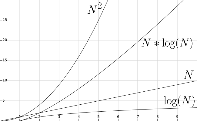
In the following, $n$ denotes the number of nodes in the tree.
In the following, $m$ denotes the length of a word and $n$ denotes the number of words in the trie.
In the following, $n$ denotes the number of nodes in the tree.
In the following, $n$ denotes the number of nodes in the graph.
In the following, $n$ denotes the number of nodes in the graph and $e$ denotes the number of edges.
In the following, $n$ denotes the number of elements in the priority queue.
We will now discuss the performance of the algorithms that we discussed in this course. When examining the performance of an algorithm we will look at the time and the space that it will require.
function PREORDER(RESULT)
    append ITEM to RESULT
    FOR CHILD in CHILDREN
           CHILD.PREORDER(RESULT)
end function
function POSTORDER(RESULT)
FOR CHILD in CHILDREN
CHILD.POSTORDER(RESULT)
append ITEM to RESULT
end functionRESULT is a variable defined and stored outside of the algorithm, it does not factor into our space requirement. Then we must account for the variables CHILD and CHILDREN. In any given iteration, CHILD will be constant and CHILDREN will have size equal to the number of children for the node we are currently at. In total, this would give us a space requirement that is linear with respect to the number of nodes.function INORDER(RESULT)
LEFTCHILD.INORDER(RESULT)
append ITEM to RESULT
RIGHTCHILD.INORDER(RESULT)
end functionRESULT is a variable defined and stored outside of the algorithm, it does not factor into our space requirement. Then we must account for the variable ITEM. This will have constant space and thus, the space requirement for the inorder traversal is constant. 1function DEPTHFIRSTSEARCH(GRAPH,SRC,TAR)
2 STACK = empty array
3 DISCOVERED = empty set
4 PARENT_MAP = empty dictionary
5 append SRC to STACK
6 while STACK is not empty
7 CURR = top of the stack
8 if CURR not in DISCOVERED
9 if CURR is TAR
10 PATH = empty array
11 TRACE = TAR
12 while TRACE is not SRC
13 append TRACE to PATH
14 set TRACE equal to PARENT_MAP[TRACE]
15 reverse the order of PATH
16 return PATH
17 add CURR to DISCOVERED
18 NEIGHS = neighbors of CURR
19 for EDGE in NEIGHS
20 NODE = first entry in EDGE
21 append NODE to STACK
22 if PARENT_MAP does not have key NODE
23 in the PARENT_MAP dictionary set key NODE with value CURR
24 return nothingSTACK can contain duplicates. In the case that we have a sparse graph, this would be bound by the number of nodes. For a dense graph however, the number of executions would be bound by the number of edges. The code within the while loop would be bound by the number of nodes because of the check that we have not already discovered the node in line 8. If we haven’t discovered it, we would take either the logic of lines 8 through 16 or lines 17 through 23 but never both in the same iteration. Both of these blocks are bound by the number of nodes in our graph. Thus the worst case time requirement would be $n^2$.STACK can contain duplicate nodes. If we have a sparse graph then it will be bound by the number of nodes. If we have a dense graph then the space is bound by the number of edges.
STACK: linear with respect to the number of edgesDISCOVERED: linear with respect to the number of nodesPARENT_MAP: linear with respect to the number of nodesCURR: 1PATH: linear with respect to the number of nodesTRACE: 1NEIGHS: linear with respect to the number of neighborsEDGE: 1NODE: 1 1function BREADTHFIRSTSEARCH(GRAPH,SRC,TAR)
2 QUEUE = empty queue
3 DISCOVERED = empty set
4 PARENT_MAP = empty dictionary
5 add SRC to DISCOVERED
6 add SRC to QUEUE
7 while QUEUE is not empty
8 CURR = first element in QUEUE
9 if CURR is TAR
10 PATH = empty list
11 TRACE = TAR
12 while TRACE is not SRC
13 append TRACE to PATH
14 set TRACE equal to PARENT_MAP[TRACE]
15 reverse the order of PATH
16 return PATH
17 NEIGHS = neighbors of CURR
18 for EDGE in NEIGHS
19 NODE = first entry in EDGE
20 if NODE is not in DISCOVERED
21 add NODE to DISCOVERED
22 if PARENT_MAP does not have key NODE
23 in the PARENT_MAP dictionary set key NODE with value CURR
24 append NODE to QUEUE
25 return nothingQUEUE will never have duplicates. Lines 1 through 6 will all execute in constant time. The while loop will occur $n$ times where $n$ is the number of nodes. Based on the logic, either 9-16 will execute or 17-24 will execute. Both of these are bound by the number of nodes in terms of time. Each iteration of the while loop will take $n$ time and we do the while loop $n$ times; thus the running time will be $n^2$.QUEUE: linear with respect to the number of nodesDISCOVERED: linear with respect to the number of nodesPARENT_MAP: linear with respect to the number of nodesCURR: 1PATH: linear with respect to the number of nodesTRACE: 1NEIGHS: linear with respect to the number of nodesEDGE: 1NODE: 1 1function KRUSKAL(GRAPH)
2 MST = GRAPH without the edges attribute(s)
3 ALLSETS = an empty list which will contain the sets
4 for NODE in GRAPH NODES
5 SET = a set with element NODE
6 add SET to ALLSETS
7 EDGES = list of GRAPH's edges
8 SORTEDEDGES = EDGES sorted by edge weight, smallest to largest
9 for EDGE in SORTEDEDGES
10 SRC = source node of EDGE
11 TAR = target node of EDGE
12 SRCSET = the set from SETS in which SRC is contained
13 TARSET = the set form SETS in which TAR is contained
14 if SRCSET not equal TARSET
15 UNIONSET = SRCSET union TARSET
16 add UNIONSET to ALLSETS
17 remove SRCSET from ALLSETS
18 remove TARSET from ALLSETS
19 add EDGE to MST as undirected edge
20 return MSTTime: The time to initialize MST would be linear with respect to the number of nodes. Regardless of the graph implementation, inserting nodes is constant time and we would do it for the number of nodes in GRAPH. Lines 4-6 would take linear time with respect to the number of nodes. Then lines 9-19 would take linear time with respect to the number of edges as it would execute $e$ times and each operation can be done in constant time, except for searching through the sets and performing set operations, which require $log_2(n)$ time. Thus, Kruskal’s algorithm will take time on the order of $e \times log_2(n)$ in the worst case.
Space:The required space for Kruskal’s algorithm is dependent on the implementation of the MST. A matrix graph would require $n^2$ space and a list graph we would require $n+e$ space.
MST: matrix graph $n^2$ or list graph $n+e$ALLSETS: linear with respect to the number of nodesNODE: 1GRAPH NODES: linear with respect to the number of nodesSET: 1EDGES: linear with respect to the number of edgesSORTEDEDGES: linear with respect to the number of edgesSRC: 1TAR: 1SRCSET: 1TARSET: 1UNIONSET: 1 1function PRIM(GRAPH, START)
2 MST = GRAPH without the edges attribute(s)
3 VISITED = empty set
4 add START to VISITED
5 AVAILEDGES = list of edges where START is the source
6 sort AVAILEDGES
7 while VISITED is not all of the nodes
8 SMLEDGE = smallest edge in AVAILEDGES
9 SRC = source of SMLEDGE
10 TAR = target of SMLEDGE
11 if TAR not in VISITED
12 add SMLEDGE to MST as undirected edge
13 add TAR to VISITED
14 add the edges where TAR is the source to AVAILEDGES
15 remove SMLEDGE from AVAILEDGES
16 sort AVAILEDGES
17 return MSTMST would be linear with respect to the number of nodes. Regardless of the graph implementation, inserting nodes is constant time and we would do it for the number of nodes in GRAPH. With a matrix graph, setting up AVAILEDGES would take linear time with respect to the number of nodes. With a list graph, this would happen in constant time. Then, we need to get the smallest edge from the AVAILEDGES list, which would be a linear time operation based on the number of edges, and we must do that once for up to each edge in the graph. So, the worst case running time for Prim’s algorithm is $e^2$. (Our implementation is actually a bit slower than this since we sort the list of available edges each time, but that is technically not necessary - our implementation is closer to $e^2 \times log_2(e)$!)MST: matrix graph $n^2$ or list graph $n+e$VISITED: linear with respect to the number of nodesAVAILEDGES: linear with respect to the number of edgesSMLEDGE: 1SRC: 1TAR: 1 1DIJKSTRAS(GRAPH, SRC)
2 SIZE = size of GRAPH
3 DISTS = array with length equal to SIZE
4 PREVIOUS = array with length equal to SIZE
5 set all of the entries in PREVIOUS to none
6 set all of the entries in DISTS to infinity
7 DISTS[SRC] = 0
8 PQ = min-priority queue
9 loop IDX starting at 0 up to SIZE
10 insert (DISTS[IDX],IDX) into PQ
11 while PQ is not empty
12 MIN = REMOVE-MIN from PQ
13 for NODE in neighbors of MIN
14 WEIGHT = graph weight between MIN and NODE
15 CALC = DISTS[MIN] + WEIGHT
16 if CALC < DISTS[NODE]
17 DISTS[NODE] = CALC
18 PREVIOUS[NODE] = MIN
19 PQIDX = index of NODE in PQ
20 PQ decrease-key (PQIDX, CALC)
21 return DISTS and PREVIOUSPQ is not empty (line 11), which is bound by the number of nodes. Thus, the block of code starting at 11 will take $n^2$ time to run in the worst case. This means that if we double the number of nodes, then the running time will be quadrupled. The worst case for Dijkstra’s algorithm is characterized by being a very dense graph, meaning each node has a lot of neighbors. If the graph is sparse and our priority queue is efficient, we could expect this running time to be more along the lines of $(n + e) \times log_2(n)$, where $e$ is the number of edges.SIZE: 1DISTS: linear with respect to the number of nodesPREVIOUS: linear with respect to the number of nodesPQ: linear with respect to the number of nodesIDX: 1MIN: 1NODE: 1NEIGHBORS: linear with respect to the number of nodesWEIGHT: 1CALC: 1PQIDX: 1A stack is a data structure with two main operations that are simple in concept. One is the push operation that lets you put data into the data structure and the other is the pop operation that lets you get data out of the structure.
A stack is what we call a Last In First Out (LIFO) data structure. That means that when we pop a piece of data off the stack, we get the last piece of data we put on the stack.
A queue data structure organizes data in a First In, First Out (FIFO) order: the first piece of data put into the queue is the first piece of data available to remove from the queue.
A list is a data structure that holds a sequence of data, such as the shopping list shown below. Each list has a head item and a tail item, with all other items placed linearly between the head and the tail.
A set is a collection of elements that are usually related to each other.
A hash table is an unordered collection of key-value pairs, where each key is unique.
The following table compares the best- and worst-case processing time for many common data structures and operations, expressed in terms of $N$, the number of elements in the structure.
| Data Structure | Insert Best | Insert Worst | Access Best | Access Worst | Find Best | Find Worst | Delete Best | Delete Worst |
|---|---|---|---|---|---|---|---|---|
| Unsorted Array | $1$ | $1$ | $1$ | $1$ | $N$ | $N$ | $N$ | $N$ |
| Sorted Array | $\text{lg}(N)$ | $N$ | $1$ | $1$ | $\text{lg}(N)$ | $\text{lg}(N)$ | $\text{lg}(N)$ | $N$ |
| Array Stack (LIFO) | $1$ | $1$ | $1$ | $1$ | $N$ | $N$ | $1$ | $1$ |
| Array Queue (FIFO) | $1$ | $1$ | $1$ | $1$ | $N$ | $N$ | $1$ | $1$ |
| Unsorted Linked List | $1$ | $1$ | $N$ | $N$ | $N$ | $N$ | $N$ | $N$ |
| Sorted Linked List | $N$ | $N$ | $N$ | $N$ | $N$ | $N$ | $N$ | $N$ |
| Linked List Stack (LIFO) | $1$ | $1$ | $1$ | $1$ | $N$ | $N$ | $1$ | $1$ |
| Linked List Queue (FIFO) | $1$ | $1$ | $1$ | $1$ | $N$ | $N$ | $1$ | $1$ |
| Hash Table | $1$ | $N$ | $1$ | $N$ | $N$ | $N$ | $1$ | $N$ |
How to analyze data and determine the appropriate data structure and algorithm!
In this module, we will discuss how we can determine which data structure we should choose when storing real-world data. We’ll typically make this decision based on the characteristics of the data we would like to store. In general, the data structures we’ve learned often work together well and complement each other, as we saw in Dijkstra’s algorithm. In some cases, one structure can be utilized to implement another, such as using a linked list to implement a stack or a queue.
When selecting a data structure for a particular data set, there are a few considerations we should keep in mind.
The first consideration is: does this data structure work for our data? To answer this, we would want to the characteristics in the data and then determine if our chosen data structure:
Once we have chosen a possible data structure, we also must consider if the choice clearly makes sense to another person who reviews our work. Some questions we may want to ask:
Finally, we should always consider the performance of our program when selecting a data structure. In some cases, the most straightforward data structure may not always be the most efficient, so at times there is a trade off between performance and simplicity. Consider the hash table structure - it may seem like a more complicated array or linked list. But, if we need to find a specific item in the structure, a hash table is typically much faster due to the use of hashes. That increase in complexity pays off in faster performance. So, when analyzing data structures for performance, we typically look at these things:
We will address this particular facet in the next chapter. For now, we will focus on the first two portions.
The first step toward determining which data structure to use relies heavily on the format of the data. By looking at the data and trying to understand what it contains and how it works, we can get a better idea of what data structure would work best to represent the data. Here, we will discuss some main types of data that we could encounter.
Unique data is the type of data where each element in a group must be unique - there can be no duplicates. However, in many cases the data itself doesn’t have a sequence or fixed ordering, we simply care if an element is present in the group or not. Some examples of unique data:
This data is best stored in the set data structure, usually built using a hash table as we learned previously.
However, many times this data may be included along with other data (a person’s ID number is part of the person’s record), so sets are rarely used in practice. Instead, we can simply modify other data structures to enforce the uniqueness property we desire on those attributes. In addition, we see this concept come up again in relational databases, where particular attributes can be assigned a property to enforce the rule that each element must be unique.
Linear data refers to data that has a sequence or fixed ordering. This can include
This data is typically stored in the array or linked list data structure, depending on how we intend to use it and what algorithms will be performed on the data.
We can think of this type of data as precisely one after another. This means that from one element there will be exactly one “next” element.
Finally, we can also adapt these data structures to represent FIFO (first-in, first-out) and LIFO (last-in, first-out) data structures using queues and stacks. As we saw previously, most implementations of queues and stacks are simply adaptations of existing linear data structures, usually the linked list.
Associative data is data where a key is associated with a value, usually in order to quickly find and retrieve the value based on its key. Some examples are:
We typically use a hash table to store this data in our programs.
However, in many cases this data could also be stored in a relational database just as easily, and in most industry programs that may also be a good choice here. Since we haven’t yet learned about relational databases, we’ll just continue to use hash tables for now.
Hierarchical data refers to data where elements can be seen as above, below, or on the same level as other elements. This can include
In contrast to linear data, hierarchical data can have multiple elements following a single element. In hierarchical data, each element has exactly one element prior to it. We typically use some form of a tree data structure to store hierarchical data.
Relational data refers to data where elements are ‘close to’ or ‘far from’ other elements. We can also think of this as ‘more similar’ and ’less similar’ as well. This can include
In a relational data set, any element can be ‘related’ to any other element. We typically use a graph data structure to store relational data.
The last type of data we will discuss is prioritized data. Here, we want to store a data element along with a priority, and then be able to quickly retrieve the element with the highest or lowest priority, depending on use. This could include:
For this data, we typically use an implementation of a priority queue based on a heap. It is important to remember that the heap does not store the data in sorted order - otherwise we would just use a linear data structure for this. Instead, it guarantees that the next element is always stored at the front of the structure for easy access, and it includes a process to quickly determine the new next element. We’ll learn a bit more about why this is so helpful in the next chapter covering performance.
It is important to note that when we are given a set of requirements for a project, the developer may not use the words to classify the types of data. Based on what a user tells us, we want to be able to infer what kind of shape the data could take.
In general, trees are good for hierarchical data. While trees can be used for linear data, it is inefficient to implement them in that way (from a certain point of view, a linked list is simply a tree where each node can only have one child). When data points have many predecessors, trees cannot be used. Thus, trees are not suitable for most relational data.
To recap, we defined a tree as having the following structure:
In this course, we used trees to represent family lineage and biologic classifications. Once we have the data in a tree, we can perform both preorder and postorder traversals to see all of the data, and we can use the structure of the tree to determine if two elements are related as ancestor and descendant or not.
We added constraints to trees to give us special types of trees, discussed below.
A trie is a type of tree with some special characteristics, which are:
Tries are best suited for data sets in which elements have similar prefixes. In this course we focused on tries to represent words in a language, which is the most common use of tries. We used tries for an auto-complete style application.

Tries are a very efficient way of storing dense hierarchical data, since each node in the trie only stores a single portion of the overall data. They also allow quickly looking up if a particular element or path exists - usually much quicker than looking through a linear list of words.
A binary tree is a type of tree with some special characteristics, which are:
Binary trees are the ideal structure to use when we have a data set with a well defined ordering. Once we have the data stored in a binary tree, we can also do an inorder traversal, which will access the elements in the tree in sorted order. We will discuss in the next chapter why we might want to choose a binary tree based on its performance.
Graphs are a good data structure for relational data. This would include data in which elements can have some sort of similarity or distance defined between those elements. This measure of similarity between elements can be defined as realistically or abstractly as needed for the data set. The distance can be as simple as listing neighbors or adjacent elements.
Graphs are multidimensional data structures that can represent many different types of data using nodes and edges. We can have graphs that are weighted and/or directed and we have introduced two ways we can represent graphs:
The first implementation of graphs that we looked at were matrix graphs. In this implementation, we had an array for the nodes and a two dimensional array for all of the possible edges.
The second implementation of graphs were list graphs. For this implementation, we had a single array of graph node objects where the graph node objects tracked their own edges.
Recall that we discussed sparse and dense graphs. Matrix graphs are better for dense graphs since a majority of the elements in the two dimensional array of edges will be filled. A great example of a dense graph would be relationships in a small community, where each person is connected to each other person in some way.
List graphs are better for sparse graphs, since each node only needs to store the outgoing edges it is connected to. This eliminates a large amount of the overhead that would be present in a matrix graph if there were thousands of nodes and each node was only connected to a few other nodes. A great example of a sparse graph would be a larger social network such as Facebook. Facebook has over a billion users, but each user has on average only a few hundred connections. So, it is much easier to store a list of those few hundred connections instead of a two dimensional matrix that has over one quintillion ($10^{18}$) elements.
In the next chapter, we will discuss the specific implications of using one or the other. However, in our requirement analysis it is important to take this into consideration. If we have relational data where many elements are considered to be connected to many other elements, then a matrix graph will be preferred. If the elements of our data set are infrequently connected, then a list graph is the better choice.
The last structure we covered were priority queues. On their own, these are good for hierarchical data. We discussed using priority queues for ticketing systems where the priority is the cost or urgency. In the project, we utilized priority queues in conjunction with Dijkstra’s algorithm.
A priority queue is a data structure which contains elements and each element has an associated priority value. The priority for an element corresponds to its importance. For this course, we implemented priority queues using heaps.
A key point of priority queues is that the priority for a value can change. This is reflected by nodes moving up (via push up) or down (via push down) through the priority queue.
In contrast, a tree has a generally fixed order. Consider the file tree as a conceptual example, it is not practical for a parent folder to switch places with a child folder.
In real world applications, it won’t always be a straightforward choice to use one structure over another. Users may come to us with unclear ideas of what they are looking for and we will need to be able to infer what structure is best suited for their needs based on what we can learn from them. Typically, those describing applications to us may not be familiar with the nomenclature we use as programmers. Instead, we have to look for clues about how the data is structured and used to help us choose the most appropriate data structures
Below we have some examples with possible solutions. We say possible solutions because there may be other ways that we could implement things. It is important that no matter what structure or algorithm we use, we should always document why we chose our answer. If someone else were to join on the project at a later time, it is important that they understand our reasoning.
A manager at a costume shop has requested that we do some data management for their online catalog. They say:
Take a moment to think on how you might go about this. Remember, there can be multiple ways of solving these problems. We need to be sure that we can articulate and justify our answers.
This is a situation where we could potentially use all three data structures!
First, we could use a tree to represent the search refinement. Thinking along the lines of a data structure, each category and subsequently each product will have exactly one parent. While something like ‘wigs’ shows up in all three categories, you wouldn’t want dog wigs showing up in a search for adult wigs. Thus, there is a unique ancestry for each category and product.

In this scenario we had a fixed ordering of our hierarchy. If the manager wanted users to be able to sort by costume part and then who it was for, our tree would not hold up.
The second portion that was requested was a recommendation system. We could implement this in two parts. The first would be a graph in which the nodes are the products and they are connected based on the similarity of the products.
For example, a purple children’s wig will be very similar to a children’s blue wig but it would be very different from an adults clown shoes. Thus, our graph would have a heavily weighted connection between the children’s purple and blue wig and there would be an edge with a very small weight between the purple wig and adult clown shoes. We can obtain this information from the manager. Since each product will be connected to every other product, a matrix graph would be best suited here.
Then once we have the graph, we could implement a priority queue. The priority queue would be built based off of the users search. When a user searches for a product, we would refer to our graph and get other similar products and enqueue them. The priority would be similarity to the searched products and the item would be the recommended product. As they continue to search, we would dequeue an element if the user selects it and we would change the priority of elements based on commonalities in the searches.
A friend approaches you about their idea for a video game and ask how they could use different data structures to produce the game. They tell us about their game which is a sandbox game with no defined goals. Users can do tasks at their own chosen speed and there is no real “completion” of the game. They say:
Take a moment to think on how you might go about this. Remember, there can be multiple ways of solving these problems. We need to be sure that we can articulate and justify our answers.
Again, this is a situation where we could potentially use three data structures!
We can use a priority queue to suggest tasks for the players to do. In this priority queue, the priority would be the payout and the item would be the task itself. As tasks get completed, we would dequeue them.
We can use a trie to represent the set of shortcuts. Below is a small sample of how we can implement our trie.

Since our friend mentioned that similar tasks should have similar combinations, a trie will fit well. These key combinations will have similar prefixes, so we can save ourselves space to store them by using a trie.
Finally, for the world layout we could use a graph. Similar to the maze project or weather station project, we can have nodes represent points on a plot and the edges will represent connections. The nodes will now have three coordinates, (x,y,z), rather than two, (x,y) or (latitude, longitude) and they will have an associated type (dirt, tree, rock, etc.).

Two nodes will be connected if they directly adjacent. Players can harvest cubes such as soil or limestone, and it would be removed from the world. We would utilize our remove node function to reflect this kind of action. Similarly, players can build up the world in spaces that allow, such as the dirt pile in an open area, and for that we can use our add node function as well as the appropriate add edge functions.
In our implementation of a graph, it would be better to use a list graph. Each block will be connected to at most six other blocks.