Introduction

YouTube Video

Video Materials

For the next data structure in the course, we will cover trees, which are used to show hierarchical data. Trees can have many shapes and sizes and there is a wide variety of data that can be organized using them. Real world data that is appropriate for trees can include: family trees, management structures, file systems, biological classifications, anatomical structures and much more.

We can look at an example of a tree and the relationships they can show. Consider this file tree; it has folders and files in folders.

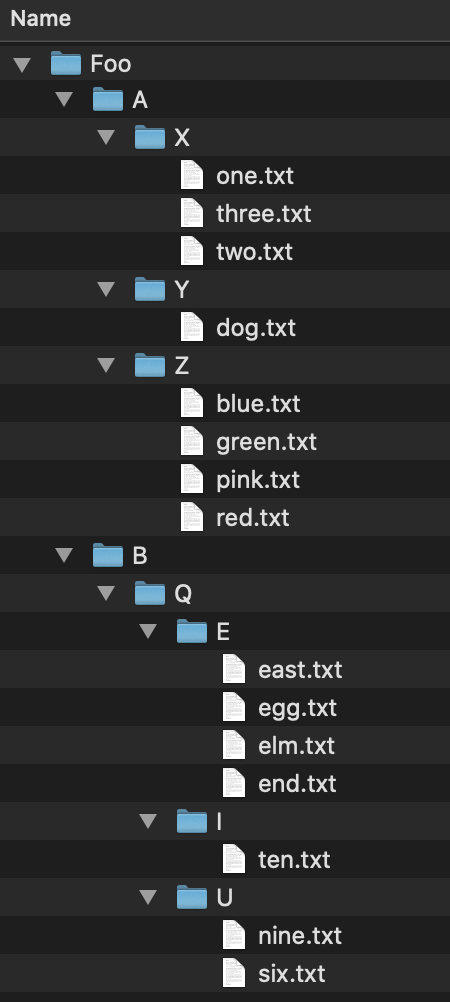
If we wanted to access the file elm.txt, we would have to follow this file path: Foo/B/Q/E/elm.txt. We can similarly store the file structure as a tree like we below. As before, if we wanted to get to the file elm.txt we would navigate the tree in the order: Foo -> B -> Q -> E -> elm.txt. As mentioned before, trees can be used on very diverse data sets; they are not limited to file trees!

What are trees?

In the last module we talked about strings which are a linear data structure. To be explicit, this means that the elements in a string form a line of characters. A tree, by contrast, is a hierarchal structure which is utilized best in multidimensional data. Going back to our file tree example, folders are not limited to just one file, there can be multiple files contained in a single folder- thus making it multidimensional.

Consider the string “abc123”; this is a linear piece of data where there is exactly one character after another. We can use trees to show linear data as well.

While trees can be used for linear data, it would be excessive and inefficient to implement them for single strings. In an upcoming module, we will see how we can use trees to represent any number of strings! For example, this tree below contains 7 words: ‘a’, ‘an’, ‘and’, ‘ant’, ‘any’, ‘all’, and ‘alp’.

In the next sections, we will discuss the properties of a tree data structure and how we would design one ourselves. Once we have a good understanding of trees and the properties of trees, we will implement our own.

General Terms

YouTube Video

Video Materials

To get ourselves comfortable in working with trees, we will outline some standard vocabulary. Throughout this section, we will use the following tree as a guiding example for visualizing the definitions.

Definitions

• Node - the general term for a structure which contains an item, such as a character or even another data structure.
• Edge - the connection between two nodes. In a tree, the edge will be pointing in a downward direction.

This tree has five edges and six nodes. There is no limit to the number of nodes in a tree. The only stipulation is that the tree is fully connected. This means that there cannot be disjoint portions of the tree. We will look at examples in the next section.

• Root - the topmost node of the tree

To be a tree, there must be exactly one root. Having multiple roots, will result in a cycle or a tree that is not fully connected. In short, a cycle is a loop in the tree.

• Parent - a node with an edge that connects to another node further from the root. We can also define the root of a tree with respect to this definition; Root: a node with no parent.
• Child - a node with an edge that connects to another node closer to the root.
  • In a general tree, the children of a node are an unordered set. There is not a fixed or defined order for generic trees. In a tree, child nodes must have exactly one parent node. If a child node has more than one parent, then a cycle will occur. If there is a node without a parent node, then this is necessarily the root node. There is no limit to the number of child nodes a parent node can have, but to be a parent node, the node must have at least one child node.

• Leaf - a node with no children. This tree has four leaves. There is no limit to how many leaves can be in a tree.

• Degree
  • Degree of a node - the number of children a node has. The degree of a leaf is zero.
  • Degree of a tree - the number of children the root of the tree has. The degree of the nodes are shown as the values on the nodes in this example. The degree of the tree is equal to the degree of the root. Thus, the degree for this tree is 2.

• A tree is defined recursively. This means that each child of the root is the root of another tree and the children of those are roots to trees as well. Again, this is a recursive definition so it will continue to the leaves. The leaves are also trees with just a single node as the root.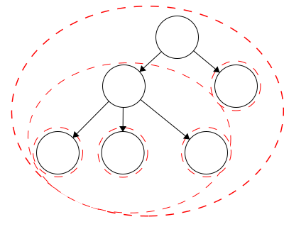
  In our example tree, we have six trees. Each tree is outlined in a red dashed circle:
  • the main tree,
    • the tree off the left of the main root,
      • the tree off the left of this root,
      • the tree in the center of this root,
      • the tree off the right of this root, and
    • the tree off the right of the main root with a single node

What Makes a Tree a Tree

YouTube Video

Video Materials

Trees can come in many shapes and sizes. There are, however some constraints to making a valid tree.

• A tree has a single root
• A child has exactly one parent
• A tree is fully connected (IE a single tree)
• A tree has no cycles (IE no loops)

Valid Trees

Any combination of the following represents a valid tree:

• A tree with a single node; just a root,

• A tree where each node has a single child, or

• A tree where nodes have many children.

Invalid Trees

Below are some examples of invalid trees.

• A cycle Again, cycles are essentially loops that occur in our tree. In this example, we see that our leaf has two parents. One way to determine whether your data structure has a cycle is if there is more than one way to get from the root to any node.

• A cycle Here we can see another cycle. In this case, the node immediately after the root has two parents, which is a clue that a cycle exists. Another test

• Two Roots Trees must have a single root. In this instance, it may look like we have a tree with two roots. Working through this, we also see that the node in the center has two parents.

• Two Trees This example would be considered two trees, not a tree with two parts. In this figure, we have two fully connected components. Since they are not connected to each other, this is not a single tree.

MyTree I

YouTube Video

Video Materials

Along with understanding how trees work, we want to also be able to implement a tree of our own. We will now outline key components of a tree class.

MyTree

Recall that trees are defined recursively so we can build them from the leaves up where each leaf is a tree itself. Each tree will have three properties: the item it contains as an object, its parent node of type MyTree, and its children as a list of MyTrees. Upon instantiation of a new MyTree, we will set the item value and initialize the parent node to None and the children to an empty list of type MyTree.

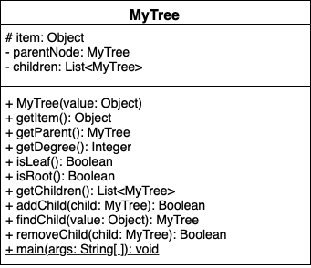
Suppose that we wanted to construct the following tree. We would start by initializing each node as a tree with no parent, no children, and the item in this instance would be the characters. Then we build it up level by level by add the appropriate children to the respective parent.

Finding a child

In this method, we will take a value as input and then check if that value is the item of a child of the current node. If the value is not the item for any of the node’s children then we should return none.

function FINDCHILD(VALUE)
    FOR CHILD in CHILDREN
        IF CHILD's ITEM is VALUE
            return  CHILD
    return NONE
end function

Getting children, item, parent, or degree

Each of these will be rather straight forward; children, item, and parent are all attributes of our node, so we can have a getter function that returns the respective values. The slightly more involved task will be getting the degree. Recall that the degree of a node is equal to the number of children. Thus, we can simply count the number of children and return this number for the degree.

Checking node type

We will have two functions to check the node type: one to determine if the node is a leaf and one to determine if it is a root. The definition of a leaf is a node that has no children. Thus, to check if a node is a leaf, we can simply check if the number of children is equal to zero. Similarly, since the definition of a root is a node with no parent, we can check that the parent attribute of the node is None.

Adding a child

YouTube Video

When we wish to add a child, we must fisrt make sure we are able to add the child.

1. Check that the child is an instance of MyTree
2. Make sure the child doesn’t already have a parent
3. Make sure the child isn’t already a child of the parent

We will return true if the child was successfully added and false otherwise while raising the appropriate errors.

function ADDCHILD(CHILD)
    IF CHILD has PARENT
        throw exception
    IF CHILD is CHILD of PARENT
        return FALSE
    ELSE
        append CHILD to PARENT's children
        set CHILD's parent to PARENT
        return TRUE
end function

As an example, lets walk through the process of building the tree above:

1. Instantiate MyTree a with item ‘A’
2. Instantiate MyTree b with item ‘B’
3. Instantiate MyTree c with item ‘C’
4. Instantiate MyTree d with item ‘D’
5. Instantiate MyTree e with item ‘E’
6. Instantiate MyTree f with item ‘F’
7. Instantiate MyTree g with item ‘G’
8. Instantiate MyTree h with item ‘H’
9. Instantiate MyTree i with item ‘I’
10. Add child tree g to tree d
11. Add child tree h to tree d
12. Add child tree i to tree d
13. Add child tree e to tree b
14. Add child tree f to tree b

Once we have completed that, visually, we would have the tree above and in code we would have:

• MyTree a with parent_node = None, item = ‘A’, children = {b,c,d}
• MyTree b with parent_node = a, item = ‘B’, children = {e,f}
• MyTree c with parent_node = a, item = ‘C’, children = { }
• MyTree d with parent_node = a, item = ‘D’, children = {g,h,i}
• MyTree e with parent_node = b, item = ‘E’, children = { }
• MyTree f with parent_node = b, item = ‘F’, children = { }
• MyTree g with parent_node = d, item = ‘G’, children = { }
• MyTree h with parent_node = d, item = ‘H’, children = { }
• MyTree i with parent_node = d, item = ‘I’, children = { }

Note: When adding a child we must currently be at the node we want to be the parent. Much like when you want to add a file to a folder, you must specify exactly where you want it. If you don’t, this could result in a wayward child.

Removing a child

YouTube Video

In the case of removing a child, we first need to check that the child we are attempting to remove is an instance of MyTree. We will return true if we successfully remove the child and false otherwise.

function REMOVECHILD(CHILD)
    IF CHILD in PARENT'S children
        REMOVE CHILD from PARENT's children
        SET CHILD's PARENT to NONE
        return TRUE
    ELSE
        return FALSE
end function

As with adding a child, we need to ensure that we are in the ‘right place’ when attempting to remove a child. When removing a child, we are not ’erasing’ it, we are just cutting the tie from parent to child and child to parent. Consider removing d from a. Visually, we would have two disjoint trees, shown below:

In code, we would have:

• MyTree a with parent_node = None, item = ‘A’, children = {b,c}
• MyTree b with parent_node = a, item = ‘B’, children = {e,f}
• MyTree c with parent_node = a, item = ‘C’, children = { }
• MyTree d with parent_node = None, item = ‘D’, children = {g,h,i}
• MyTree e with parent_node = b, item = ‘E’, children = { }
• MyTree f with parent_node = b, item = ‘F’, children = { }
• MyTree g with parent_node = d, item = ‘G’, children = { }
• MyTree h with parent_node = d, item = ‘H’, children = { }
• MyTree i with parent_node = d, item = ‘I’, children = { }

Summary

In this module we have introduce vocabulary related to trees and what makes a tree a tree. To recap, we have introduced the following:

• Child - a node with an edge that connects to another node closer to the root.
• Degree
  • Degree of a node - the number of children a node has. The degree of a leaf is zero.
  • Degree of a tree - the number of children the root of the tree has.
• Edge - connection between two nodes. In a tree, the edge will be pointing in a downward direction.
• Leaf - a node with no children.
• Node - the general term for a structure which contains an item, such as a character or even another data structure.
• Parent - a node with an edge that connects to another node further from the root. We can also define the root of a tree with respect to this definition;
• Root - the topmost node of the tree; a node with no parent.

Now we will work on creating our own implementation of a tree. These definitions will serve as a resource to us when we need refreshing on meanings; feel free to refer back to them as needed.

Introduction

In the last module, we covered the underlying vocabulary of trees and how we can implement our own tree. To recall, we covered: node, edge, root, leaf, parent, child, and degree.

For this module we will expand on trees and gain a better understanding of how powerful trees can be. As before, we will use the same tree throughout the module for a guiding visual example.

Terms I

YouTube Video

Many of the terms used in trees relate to terms used in family trees. Having this in mind can help us to better understand some of the terminology involved with abstract trees. Here we have a sample family tree.

• Ancestor - The ancestors of a node are those reached from child to parent relationships. We can think of this as our parents and our parent’s parents, and so on.
  • Let’s look at all of the ancestors of each of our nodes in the family tree.
    • Ava’s ancestors: Uzzi, Joe, Myra. This is because, Uzzi is the parent of Ava, Joe is the parent of Uzzi, and Myra is the parent of Joe. Try to work out the following and click the name to reveal the ancestors.
    Uma:

    Zia, Myra - **Zia** is the parent of Uma and **Myra** is the parent of Zia.
    Myra:

    None - Myra does not have a parent node.
    Raju:

    Myra - **Myra** is the parent of Raju.
    Bev:

    Uzzi, Joe, Myra - **Uzzi** is the parent of Bev, **Joe** is the parent of Uzzi, and **Myra** is the parent of Joe.
• Descendant - The descendants of a node are those reached from parent to child relationships. We can think of this as our children and our children’s children and so on.
  • Let’s look at all of the descendants of each of our nodes in the family tree.
    • Ava’s descendants: None. Ava has no child nodes and thus, no descendants. Try to work out the following and click the name to reveal the descendants.
    Uma:

    Ang - **Ang** is the child of Uma
    Myra:

    Raju, Joe, Zia, Uzzi, Bert, Uma, Bev, Ava, Ang, Isla, Eoin - All of the nodes in a tree will be descendants of the root. To work it out: **Raju, Joe** and **Zia** are the children of Myra, **Uma** is the child of Zia, **Ang** is the child of Uma, and we can work the rest out for Joe's children.
    Raju:

    None - Raju has no child nodes.
    Bev:

    Isla, Eoin - **Isla** is the child of Bev and **Eoin** is the child of Isla.
• Siblings - Nodes which share the same parent
  • We can think about the siblings of all of our nodes in the family tree.
    • Ava’s siblings: Bev - Uzzi is the parent node of Ava; Uzzi has two child nodes, Ava and Bev. Try to work out the following and click the name to reveal the siblings.
    Uma:

    None - Zia is the parent node of Uma; Zia has only one child node, Uma.
    Myra:

    None - Myra is the root and thus does not have a parent node resulting in no siblings.
    Raju:

    Joe, Zia - Myra is the parent node of Raju; Myra has three child nodes, **Joe**, **Zia**, and Raju
    Bev:

    Ava - Uzzi is the parent node of Bev; Uzzi has two child nodes, Bev and **Ava**.

Recursion Refresh

YouTube Video

In principle, the recursive case breaks the problem down into smaller portions until we reach the base case. Recursion presents itself in many ways when dealing with trees.

Trees are defined recursively with the base case being a single node. Then we recursively build the tree up. With this basis for our trees, we can define many properties using recursion rather effectively.

Terms II

YouTube Video

We can describe the sizes of trees and position of nodes using different terminology, like level, depth, and height.

• Level - The level of a node characterizes the distance between the node and the root. The root of the tree is considered level 1. As you move away from the tree, the level increases by one.
  • For our family tree example, what nodes are in the following levels? Think about the answer and then click corresponding arrow.
    Level 1:

    Myra - Level 1 is always the root
    Level 2:

    Raju, Joe, Zia - These are the nodes which are 1 edge away from the root.
    Level 3:

    Uzzi, Bert, Uma - These are the nodes which are 2 edges away from the root.
    Level 4:

    Bev, Ava, Ang - These are the nodes which are 3 edges away from the root.
    Level 5:

    Isla - This is the only node which is 4 edges away from the root.
    Level 6:

    Eoin - This is the only node which is 5 edges away from the root.
• Depth - The depth of a node is its distance to the root. Thus, the root has depth zero. Level and depth are related in that: level = 1 + depth.
  • For our family tree example, what nodes have the following depths?
    Depth 0:

    Myra - The root will always be at depth 0.
    Depth 1:

    Raju, Joe, Zia - These are the nodes which are 1 edge away from the root.
    Depth 2:

    Uzzi, Bert, Uma - These are the nodes which are 2 edge away from the root.
    Depth 3:

    Bev, Ava, Ang - These are the nodes which are 3 edge away from the root.
    Depth 4:

    Isla - This is the only node which is 4 edges away from the root.
    Depth 5:

    Eoin - This is the only node which is 5 edges away from the root.
• Height of a Node - The height of a node is the longest path to a leaf descendant. The height of a leaf is zero.
  • For our family tree example, what nodes have the following heights?
    Height 0:

    Raju, Eoin, Ava, Bert, Ang - The leaves always have height 0.
    Height 1:

    Isla, Uma - `Isla -> Eoin` and `Uma -> Ang`
    Height 2:

    Bev, Zia - `Bev -> Isla -> Eoin` and `Zia -> Uma -> Ang`
    Height 3:

    Uzzi - `Uzzi -> Bev -> Isla -> Eoin`
    Height 4:

    Joe - `Joe -> Uzzi -> Bev -> Isla -> Eoin`
    Height 5:

    Myra - `Myra -> Joe -> Uzzi -> Bev -> Isla -> Eoin`
• Height of a Tree - The height of a tree is equal to the height of the root.
  • Our family tree would have height 5

Terms III

YouTube Video

When working with multidimensional data structures, we also need to consider how they would be stored in a linear manner. Remember, pieces of data in computers are linear sequences of binary digits. As a result, we need a standard way of storing trees as a linear structure.

• Path - a path is a sequence of nodes and edges, which connect a node with its descendant. We can look at some paths in the tree above:

  • From Q to O: QRO
  From `Q` to `Y`:

  `QWY`
  From `R` to `P`:

  `RP`

• Traversal is a general term we use to describe going through a tree. The following traversals are defined recursively.

Preorder Traversal

1. Access the root, record its value.
2. Run the preorder traversal each of the children

YouTube Video

• The Pre refers to the root, meaning the root goes before the children.
• Remember: Root Children
• For the above tree, the preorder traversal could result in: QWYUERIOPTA

Postorder Traversal

1. Run the postorder traversal on each of the children
2. Access the root, record its value

YouTube Video

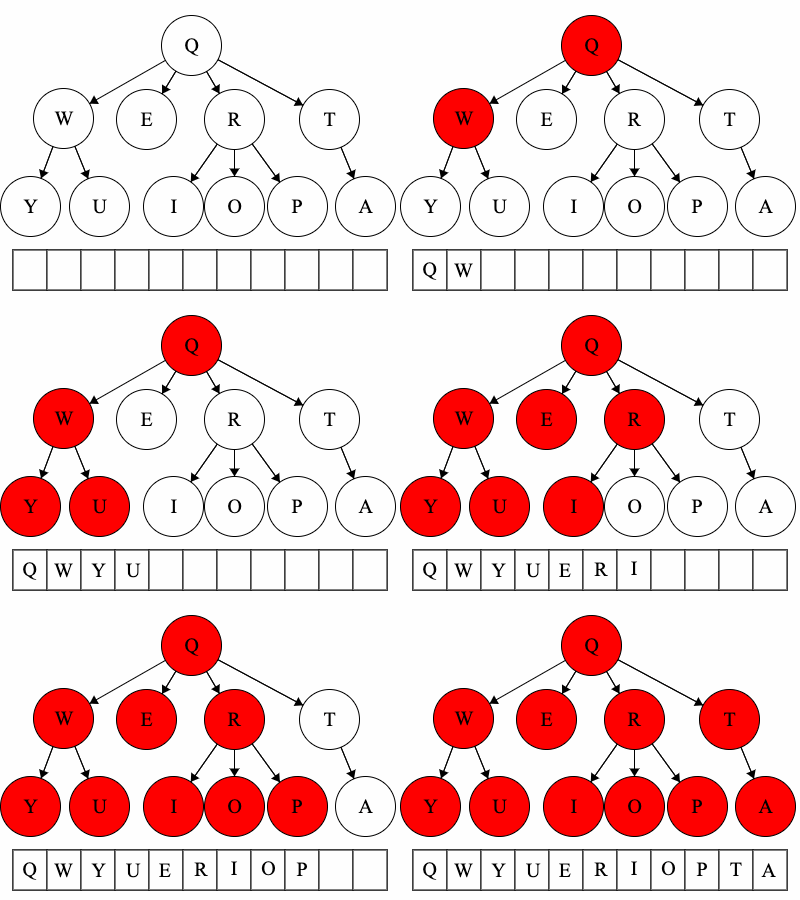
• The Post refers to the root, meaning the root goes after the children.
• Remember: Children Root
• For the above tree, the postorder traversal could result in: YUWEIOPRATQ

When we talk about traversals for general trees we have used the phrase ’the traversal could result in’. We would like to expand on why ‘could’ is used here. Each of these general trees are the same but their traversals could be different. The key concept in this is that for a general tree, the children are an unordered set of nodes; they do not have a defined or fixed order. The relationships that are fixed are the parent/child relationships.

MyTree Recursive I

Again, we want to be able to implement a working version of a tree. From the last module, we had functions to add children, remove children, get attributes, and instantiate MyTree. We will now build upon that implementation to create a true tree.

MyTree with recursion

Recall that in the previous module, we were not yet able to enforce the no cycle rule. We will now enforce this and add other tree functionality.

In the first module, we discussed how we can define trees recursively, meaning a tree consists of trees. We looked at the following example. Each red dashed line represented a distinct tree, thus we had five trees within the largest tree making six trees in total.

We will use our existing implementation from the first module. Now to make our tree recursive, we will include more getter functions as well as functions for traversals and defining node relationships.

Get depth, height, size, and root

We can define each of these recursively.

YouTube Video

Get Depth

• Depth - The depth of a node is its distance to the root. Thus, the root has depth zero.

We can define the depth of a node recursively:

• Base case: we are at the root and the depth is zero
• Recursive case: for any other node, the depth is 1 plus the depth of the parent

function GETDEPTH()
    if ROOT
        return 0
    else 
        return 1 + PARENT.GETDEPTH()
end function

Get Height

• Height of a Node - The height of a node is the longest path to a leaf descendant. The height of a leaf is zero.

We can define the height of a node recursively:

• Base case: we are at the leaf and the height is zero
• Recursive case: for any other node, return 1 plus the maximum height of its children

function GETHEIGHT()
    if LEAF
        return 0
    else 
        MAX = 0
        for CHILD in CHILDREN
            CURR_HEIGHT = CHILD.GETHEIGHT()
            if CURR_HEIGHT > MAX
                MAX = CURR_HEIGHT
        return 1 + MAX
end function

Get Root

• Root - the topmost node of the tree; a node with no parent.

We can define returning the root recursively:

• Base case: we are at the root so return it
• Recursive case: for any other node, return the root of the nodes parent

function GETROOT()
    if ISROOT()
        return this tree
    else
        return PARENT.GETROOT()
end function

Get Size

We define the size of a tree as the total number of children.

function GETSIZE()
    SIZE = 1
    for CHILD in CHILDREN
        SIZE += CHILD.GETSIZE()
    return SIZE
end function

Find a Value

To find a value within our tree, we will traverse down a branch as far as we can until we find the value. This will return the tree that has the value as the root.

function FIND(VALUE)
	if ITEM is VALUE
		return this node
	for CHILD in CHILDREN
		FOUND = CHILD.FIND(VALUE)
		if FOUND is not NONE
			return FOUND
	return NONE
end function

MyTree Recursive II

Determine relationships (Ancestor, Descendant, Sibling)

We can determine many relationships within the tree. For example, given a node is it an ancestor of another node, a descendant, or a sibling?

YouTube Video

Is Ancestor?

For this function, we are asking: is this node an ancestor of the current instance? In this implementation, we will start at our instance and work down through the tree trying to find the node in question. With that in mind, we can define this process recursively:

• Base case: we are at the node in question, so return true OR we are at a leaf so return false.
• Recursive case: run the method from each of the children of the node.

function ISANCESTOR(TREE)
    if at TREE
        return true
    else if at LEAF
        return false
    else 
        for CHILD in CHILDREN
            FOUND = CHILD.ISANCESTOR(TREE)
            if FOUND
                return true
        return false
end function

Is Descendant?

For this function, we are asking: is this node a descendant of the current instance? In this implementation, we will start at our instance and work up through the tree trying to find the node in question. With that in mind, we can define this process recursively:

• Base case: we are at the node in question, so return true OR we are at the root so return false.
• Recursive case: run the method from the parent of the node.

function ISDESCENDANT(TREE)
    if at TREE
        return true
    else if at ROOT
        return false
    else 
        return PARENT.ISDESCENDANT(TREE)
end function

Is Sibling?

For this function, we are asking: is this node a sibling of the current instance? To determine this, we can get the parent of the current instance and then get the parents children. Finally, we check if the node in question is in that set of children.

function ISSIBLING(TREE)
    if TREE in PARENT's CHILDREN
        return true
    else 
        return false
end function

Lowest common ancestor

In any tree, we can say that the root is a common ancestor to all of the nodes. We would like to get more information about the common ancestry of two nodes. For this function, we are asking: which node is the first place where this instance and the input node’s ancestries meet? Similar to our ISDESCENDANT, we will work our way up the tree to find the point where they meet

• Base case: we are at our tree so return the tree OR we are at an ancestor of our tree so return the instance OR we are at the root so return nothing
• Recursive case: run the method from the parent.

function LOWESTANCESTOR(TREE)
    if at TREE
        return TREE
    else if ISANCESTOR(TREE)
        return instance
    else if at ROOT
        return NONE
    else
        return PARENT.LOWESTANCESTOR(TREE)
end function

Path from the root

This function will generate the path which goes from the root to the current instance.

function PATHFROMROOT(PATH)
    if NOT ROOT
        PARENT.PATHFROMROOT(PATH)
    append ITEM to PATH
end function

MyTree Recursive III

Traversals

In this module we have talked about two traversals: preorder and postorder. Both of these are defined recursively and the prefix refers to the order of the root.

Preorder

In a preorder traversal, first we access the root and then run the preorder traversal on the children.

function PREORDER(RESULT)
    append ITEM to RESULT
    FOR CHILD in CHILDREN
           CHILD.PREORDER(RESULT)
end function

Postorder

In a postorder traversal, first we run the postorder traversal on the children then we access the root.

function POSTORDER(RESULT)
   FOR CHILD in CHILDREN
           CHILD.POSTORDER(RESULT)
   append ITEM to RESULT
end function

Summary

In this section, we discussed more terminology related to trees as well as tree traversals. To recap the new vocabulary:

• Ancestor - The ancestors of a node are those reached from child to parent relationships. We can think of this as our parents and the parents of our parents, and so on.
• Depth - The depth of a node is its distance to the root. Thus, the root has depth zero. Level and depth are related in that: level = 1 + depth.
• Descendant - The descendants of a node are those reached from parent to child relationships. We can think of this as our children and our children’s children and so on.
• Height of a Node - The height of a node is the longest path to a leaf descendant. The height of a leaf is zero.
• Height of a Tree - The height of a tree is equal to the height of the root.
• Level - The level of a node characterizes the distance the node is from the root. The root of the tree is considered level 1. As you move away from the tree, the level increases by one.
• Path - a sequence of nodes and edges which connect a node with its descendant.
• Siblings - Nodes which share the same parent
• Traversal is a general term we use to describe going through a tree. The following traversals are defined recursively.
  • Preorder Traversal (Remember: Root Children):
    1. Access the root
    2. Run the preorder traversal on the children
  • Postorder Traversal (Remember: Children Root):
    1. Run the postorder traversal on the children
    2. Access the root.

Tries

YouTube Video

Recall that in the beginning of our discussions about trees, we looked at a small tree which contained seven strings as motivation for trees. This was a small example of a trie (pronounced ’try’) which is a type of tree that can represent sets of words.

Tries can be used for a variety of tasks ranging from leisurely games to accessibility applications. One example is ‘Boggle’ where players have a set of random letters and try to make as many words as possible. To code this game, we could create a vocabulary with a trie then traverse it to determine if players have played legal words. We can also use tries to provide better typing accessibility. Users could type a few letters of a word and our code could traverse the trie and suggest what letters or words they may be trying to enter.

A trie is a type of tree with some special characteristics. First it must follow the guidelines of being a tree:

• There must be a single root,
• Each child node has a single parent node,
• It must be fully connected (no disjoint parts), and
• There can be no cycles (no loops).

The special characteristics for tries are:

• By starting at the root and traversing parent to children relationships we can build user-defined words, and
• Each node has a boolean property to indicate if it is the end of a word.

In this course, we will display nodes with two circles as a convention to show which nodes are the end of words. Looking at this small trie as an example, we can determine which words are contained in our trie. We start at the root, which will typically be an empty string, and traverse to a double lined node. "" -> a -> l -> l. Thus, the word ‘all’ is contained in our trie. Words within our tries do not have to end at leaves. For example, we can traverse "" -> a for the word ‘a’. We say this trie ‘contains’ seven words: ‘a’, ‘an’, ‘and’, ‘ant’, ‘any’, ‘all’, and ‘alp’.

Trie Example

Let’s look at another example of a trie. Here we have a larger trie. Think about how many words are captured by the tree; click the tree to see how many!

While the ‘a’, ‘at’, and ‘bee’ are words in the English language, they are not recognized by our trie. Depending on what the user intended, this could be by design. When we build our tries, users will input words that are valid for their vocabulary. Tries are not limited to the English language and can be created for any vocabulary.

MyTrie I

To implement our own trie, we will build off of MyTree that we built recursively. We will add an attribute to our tree to reinforce which nodes are words and which ones are not.

Attributes

We have the existing attributes of MyTree: parent, children, and item. For MyTrie, we introduce the boolean attribute is_word to delineate if our trie is a word.

Adding a Word

YouTube Video

To add a word to our trie, we traverse through the trie letter by letter. We can define this recursively.

• Base Case: length of the word is zero and it was already a word in our trie, return false (because we did not add the word) OR length of the word is zero and it is not already a word in our trie, set the boolean for the node at the end of the word to true and return true
• Recursive case: split the string into the first character and the rest. Get the node of the first letter of the string; if it does not exist create it, then run the add word function on the remainder of the string.

function ADDWORD(WORD)
    if WORD length is 0
        if already a word
            return false
        else
            set is_word to true
            return true
    else
        FIRST = first character of WORD
        REMAIN = remainder of WORD
        CHILD = FINDCHILD(FIRST)
        if CHILD is NONE
            NODE = new MyTrie with item equal FIRST
            insert NODE into our existing trie 
            CHILD = NODE
        return CHILD.ADDWORD(REMAIN)
end function

Removing a Word

YouTube Video

Similar to adding a word, we traverse our trie letter by letter. Once we get to the end of the word set is_word to false. If the word ends at a leaf, we will remove the leaf (then if the second to last character is a leaf, we remove the leaf and so on). If the word does not end in a leaf, meaning another word uses that node, we will not remove the node.

• Base Case: length of the word is zero and it was not a word in our trie, return false (because we did not remove the word) OR length of the word is zero and it is already a word in our trie, set the boolean for the node at the end of the word to false and return true
• Recursive case: split the string into the first character and the rest. Get the node of the first letter of the string, if that node does not exist, return false (because we did not remove the word). If the node does exist run remove word on the child for the remainder of the word. After that, if the node’s is_word is false and it is a leaf, remove the node.

function REMOVEWORD(WORD)
    if WORD length is 0
        if already not a word
            return false
        else
            set is_word to false
            return true
    else
        FIRST = first character of WORD
        REMAIN = remainder of WORD
        CHILD = FINDCHILD(FIRST)
        if CHILD is NONE
            return false
        else
            RET = CHILD.REMOVEWORD(REMAIN)
            if CHILD is not a word AND CHILD is a leaf
                REMOVECHILD(CHILD)
            return RET
end function

Check if trie contains word

YouTube Video

Again, we will traverse the trie letter by letter. Once we get to the last letter, we can return that nodes is_word attribute. There is a chance that somewhere in our word, the letter is not a child of the previous node. If that is the case, then we return false.

function CONTAINSWORD(WORD)
    if WORD length is 0
        return `is_word`
    else
        FIRST = first character of WORD
        REMAIN = remainder of WORD
        CHILD = FINDCHILD(FIRST)
        if CHILD is NONE
            return false
        else
            return CHILD.CONTAINSWORD(REMAIN)
end function

MyTrie II

Getters

YouTube Video

Getting word count

For this function, we want to get the total number of words that are contained within our trie. We will fan out through all of the children and count all of the nodes that have their is_word attribute equal to true.

function WORDCOUNT()
    COUNT = 0
    if is_word
        COUNT = 1
    for CHILD in CHILDREN
        COUNT += CHILD.WORDCOUNT()
    return COUNT
end function

Get max word length

Next, we want to get the longest word contained in our trie. To do this, we will recurse each child and find the maximum length of the child.

• Base Case: we are at a leaf and it is a word, return 0
• Recursive Case: declare a maximum of -1 for a tracker and then for each child run the maximum word length function on it. If the value returned from the child is greater than our maximum tracker, set the tracker equal to the value. Once we have iterated all of the children, return the maximum tracker plus one.

function MAXWORD()
    if LEAF and is_word
        return 0
    else
        MAX = -1
        for CHILD in CHILDREN
            COUNT = CHILD.MAXWORD()
            if COUNT greater than MAX
                MAX = COUNT
        return MAX + 1
end function

Get completions

YouTube Video

This function will act as an auto-complete utility of sorts. A user will input a string of characters and we will return all of the possible words that are contained in our trie. This will happen in two phases. First, we traverse the trie to get to the end of the input string (lines 1-12). The second portion then gets all of the words that are contained after that point in our trie (lines 14-21).

function COMPLETIONS(WORD)
1.    if WORD length greater than 0
2.        FIRST = first character of WORD
3.        REMAIN = remainder of WORD
4.        CHILD = FINDCHILD(FIRST)
5.        if CHILD is none
6.            return []
7.        else
8.            COMPLETES = CHILD.COMPLETIONS(REMAIN)
9.            OUTPUT = []
10.            for COM in COMPLETES
11.                append CHILD.item + COM to OUTPUT
12.            return OUTPUT
13.    else
14.        OUTPUT = []
15.        if is_word
16.            append ITEM to OUTPUT
17.        for CHILD in CHILDREN
18.            COMPLETES = CHILD.COMPLETIONS("")
19.            for COM in COMPLETES
20.                append CHILD.item + COM to OUTPUT
21.        reutrn OUTPUT
end function

Binary Tree

YouTube Video

A binary tree is a type of tree with some special conditions. First, it must follow the guidelines of being a tree:

• There must be single root,
• each child node must have a single parent node,
• it must be fully connected (no disjoint parts), and
• there can be no cycles (no loops).

The special conditions that we impose on binary trees are the following:

• Each node has at most 2 children (nodes can have 0, 1, or 2 children), and
• unlike general trees, the children in a binary tree are not an unordered set. The children must be ordered such that:
  • all of the descendants in the left tree are less than the parent’s value, and
  • all of the descendants in the right tree are greater than the parent’s value

To reinforce these concepts, we will look at examples of binary trees and examples that are not binary trees.

Binary Tree Examples

YouTube Video

Valid Binary Trees

This is a valid binary tree. We have a single node, the root, with no children. As with general trees, binary trees are built recursively. Thus, each node and its child(ren) are trees themselves.

This is also a valid binary tree. All of the left children are less than their parent. The node with item ‘10’ is also in the correct position as it is less than 12, 13, and 14 but greater than 9.

We have the same nodes but our root is now 12 whereas before it was 14. This is also a valid binary tree.

Here we have an example of a binary tree with alphabetical items. As long as we have items which have a predefined order, we can organize them using a binary tree.

Invalid Binary Trees

We may be inclined to say that this is a binary tree: each node has 0, 1, or 2 children and amongst children and parent nodes, the left child is smaller than the parent and the right child is greater than the parent. However, in binary trees, all of the nodes in the left tree must be smaller than the root and all of the nodes in the right tree must be larger than the root. In this tree, D is out of place. Node D is less than node T but it is also less than node Q. Thus, node D must be on the right of node Q.

In this case, we do not have a binary tree. This does fit all of the criteria for being a tree but not the criteria for a binary tree. Nodes in binary trees can have at most 2 children. Node 30 has three children.

Traversals

YouTube Video

In the first module we discussed two types of traversals: preorder and postorder. Within that discussion, we noted that for general trees, the preorder and postorder traversal may not be unique. This was due to the fact that children nodes are an unordered set.

Recall that these were defined as such:

• Preorder Traversal (Remember: Root Children):
  1. Access the root
  2. Run the preorder traversal on the children
• Postorder Traversal (Remember: Children Root):
  1. Run the postorder traversal on the children
  2. Access the root.

Now for binary trees, we can modify their definitions to be more explicit:

• Preorder Traversal (Remember: Root Left Right):
  1. Access the root
  2. Run the preorder traversal on the left child
  3. Run the preorder traversal on the right child
• Postorder Traversal (Remember: Left Right Root):
  1. Run the postorder traversal on the left child
  2. Run the postorder traversal on the right child
  3. Access the root.

Let’s practice traversals on the following binary tree.

Preorder Traversal

Postorder Traversal

In-Order Traversal

YouTube Video

Since we have fixed order on the children, we can introduce another type of traversal: in-order traversal.

• In-order Traversal:

  1. Run the in-order traversal on the left child
  2. Access the root, write its value
  3. Run the in-order traversal on the right child
  • Remember: Left Root Right

MyBinaryTree

YouTube Video

Our implementation of binary trees will inherit from our MyTree implementation as binary trees are types of trees. Thus, MyBinaryTree will have the functionality of MyTree in addition to the following.

Attributes

The binary tree has two attributes

• Left Child: an instance of MyBinaryTree, the item should be less than the item of the parent.
• Right Child: an instance of MyBinaryTree, the item should be greater than the item of the parent.

Miscellaneous Functions

• Get Size

  • Will override the MyTree size function. If the tree is empty then we return zero. If the tree is not empty then call the MyTree size function.

• Is Empty

  • Will return true if the node we have called the function from is empty and false if otherwise.

• To Sorted List

  • Will get all of the nodes items and sort them

function TOSORTEDLIST()
    LIST = []
    if there`s LEFTCHILD
        LIST = LIST + LEFTCHILD.TOSORTEDLIST
    LIST = LIST + ITEM
    if there`s RIGHTCHILD
        LIST = LIST + RIGHTCHILD.TOSORTEDLIST
    return LIST

Inserting Children

YouTube Video

When inserting children to a binary tree, we must take some special considerations. All of the node items in the left tree must be less than the parent node item and all of the node items in the right tree must be greater than the parent node item.

The general procedure for adding a child is the following:

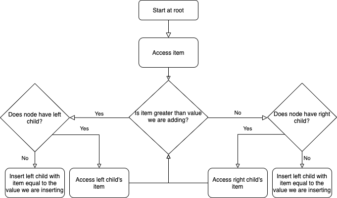
Suppose that we have the following tree and we want to add a node with item ‘85’. Click the binary tree to see the resulting tree.

function INSERT(VALUE)
    if node is empty:
        set nodes item to value
    else:
        if node.ITEM is VALUE
            return false
        else if node.ITEM > VALUE 
            LC = node`s left child
            if LC is NONE
                CHILD = new BINARYTREE with root.ITEM equal VALUE
                add CHILD to nodes children
                set node.LEFTCHILD equal to CHILD
                return true
            else
                return LC.INSERT(VALUE)
        else
            RC = node`s right child
            if RC is NONE
                CHILD = new BINARYTREE with root.ITEM equal VALUE
                add CHILD to nodes children
                set node.RIGHTCHILD equal to CHILD
                return true
            else
                return RC.INSERT(VALUE)
end function

Removing Children

YouTube Video

Removing children is not as straightforward as inserting them. The general procedure for removing a child is to replace that nodes value with its smallest right descendant. First we will traverse the binary tree until we find the node with the value we are trying to remove (lines 18-32 below). Then we have three separate cases, discussed in detail below.

Removing a Leaf

Removing a leaf is the most straightforward. We remove the value from the node and then sever the connection between parent and child. (lines 5-7 below)

Suppose we have this binary tree and we want to remove value 5. What do you think the resulting binary tree will look like? Click the binary tree to see the result.

Removing a Node without Right Child

When we remove a value from a node that does not have a right child, we cannot replace the value with the smallest right child. In this instance we will instead replace the value with the smallest left child then prune the tree to clean it up. Once we replace the value, we must switch the node’s left child to be the right child in order to maintain proper binary tree structure. (lines 8-13 below)

Suppose we have this binary tree and we want to remove value 4. What do you think the resulting binary tree will look like? Click the binary tree to see the result.

Removing a Node with Right Child

When we remove a value from a node that has a right child, we can replace the value with the nodes smallest right child. (Lines 14-17 Below)

Suppose we have this binary tree and we want to remove value 10. What do you think the resulting binary tree will look like? Click the binary tree to see the result.

Complete Pseudocode

1. function REMOVE(VALUE)
2.    if node is empty:
3.        error
4.    if node.ITEM is VALUE
5.        if node is a leaf
6.            set node.ITEM to none
7.            return TRUE
8.        else if node has no right child
9.            node.ITEM = LEFTCHILD.REMOVESMALLEST()
10.           prune left-side
11.           store left child in right child
12.           set left child to none    
13.           return TRUE
14.        else
15.            node.ITEM = RIGHTCHILD.REMOVESMALLEST()
16.            prune right-side
17.            return TRUE
18.    else
19.        if node.ITEM > VALUE
20.            if node has LEFTCHILD
21.                SUCCESS = LEFTCHILD.REMOVE(VALUE)
22.                prune left-side
23.                return SUCCESS
24.            else
25.                return FALSE
26.        else
27.            if node has RIGHTCHILD
28.                SUCCESS = RIGHTCHILD.REMOVE(VALUE)
29.                prune right-side
30.                return SUCCESS
31.            else
32.                return FALSE
33. end function

Extras for Removal

We use the pruning functions to severe the tie between parent and child nodes.

function PRUNERIGHT()
    if RIGHTCHILD has no value
        REMOVECHILD(RIGHTCHILD)
        set this nodes RIGHTCHILD former RIGHTCHILDs RIGHTCHILD
        if RIGHTCHLID is not none
            ADDCHILD(RIGHTCHILD)
end function

function PRUNELEFT()
    if LEFTCHILD has no value
        REMOVECHILD(LEFTCHILD)
        set this nodes LEFTCHILD former LEFTCHILDs RIGHTCHILD
        if LEFTCHILD is not none
            ADDCHILD(LEFTCHILD)
end function

We use the remove smallest function to retrieve the smallest value in the binary tree which will replace our value.

function REMOVESMALLEST()
    if node has left child
        REPLACEMENT = LEFTCHILD.REMOVESMALLEST
        prune left-side
        return REPLACEMENT
    else
        REPLACEMENT = node.ITEM
        if node has right child
            node.ITEM = RIGHTCHILD.REMOVESMALLEST()
            prune right-side
        else
            node.ITEM = NONE
        return REPLACEMENT
end function

Balance

While this is a valid binary tree, it is not balanced. Let’s look at the following tree.

We have the same nodes but our root is now 12 whereas before it was 14. This is a valid binary tree. We call this a balanced binary tree. A balanced binary tree looks visually even amongst the left and right trees in terms of number of nodes.

Note: Balancing is not necessary for a valid binary tree. It is, however, important in terms of time efficiency to have a balanced tree. For example, the number of actions when inserting an element is about the same as the number of levels in the tree. If we tried to add the value 11 into the unbalanced tree, we would traverse 5 nodes. If we tried to add the value 11 in to the balanced tree, we would traverse just 3 nodes.

We believe that balancing binary trees is out of the scope of this course. If you are interested in how we might balance a tree, feel free to check out these videos by Dr. Joshua Weese.

YouTube Video

YouTube Video