Graphs: Searching and Traversing
Welcome!
This page is the main page for Graphs: Searching and Traversing
This page is the main page for Graphs: Searching and Traversing
In the previous modules, we have introduced graphs and two implementations. This module will cover the traversals through graphs as well as path search techniques.
As we have discussed previously, graphs can have many applications. Based on that, there are many things that we may want to infer from graphs. For example, if we have a graph that depicts a railroad or electrical network, we could determine what maximum flow of the network. The standard approach for this task is the Ford-Fulkerson Algorithm. In short, given a graph with edge weights that represent capacities the algorithm will determine the maximum flow throughout the graph.
From the matrix graph module, we used the following distribution network as an example.

Conceptually, we would want to determine the maximum number of units that could leave the distribution center without having excess laying around stores. Using the maximum flow algorithm, we would determine that the maximum number of units would be 15.
The driving force in the Ford-Fulkerson algorithm, as well as other maximum flow algorithms, is the ability to find a path from a source to a target. Specifically, these algorithms use breadth first and depth first searches to discover possible paths.
To get to introducing the searches, we will first discuss the basis of them. Those are the depth first traversal and the breadth first traversal. We will outline the premise of these traversals and then discuss how we can modify their algorithms for various tasks, such as path searches.
We can perform these traversals on any type of graph. Conceptually, it will help to have a tree-like structure in mind to differentiate between depth first and breadth first.
First we will discuss Depth First Traversal. We can define the depth first traversal in two ways, iteratively or recursively. For this course, we will define it iteratively.
In the iterative algorithm, we will initialize an empty stack and an empty set. The stack will determine which node we search next and the set will track which nodes we have already searched.
Recall that a stack is a ‘Last In First Out’ (LIFO) structure. Based on this, the depth first traversal will traverse a nodes descendants before its siblings.
To do the traversal, we must pick a starting node; this can be an arbitrary node in our graph. If we were doing the traversal on a tree, we would typically select the root at a starting point. We start a while loop to go through the stack which we will be pushing and popping from. We get the top element of the stack, if the node has not been visited yet then we will add it to the set to note that we have now visited it. Then we get the neighbors of the node and put them onto the stack and continue the process until the stack is empty.
function DEPTHFIRST(GRAPH,SRC)
    STACK = empty array
    DISCOVERED = empty set
    append SRC to STACK
    while STACK is not empty
        CURR = top of the stack
        if CURR not in DISCOVERED
            add CURR to DISCOVERED
            NEIGHS = neighbors of CURR
            for EDGE in NEIGHS
                NODE = first entry in EDGE
                append NODE to STACK
Since the order of the neighbors is not guaranteed, the traversal on the same graph with the same starting node can find nodes in different orders.
We can also perform a breadth first traversal either iteratively or recursively. As with the depth first traversal, we will define it iteratively.
In the iterative algorithm, we initialize an empty queue and an empty set. Like depth first traversal, the set will track which nodes we have discovered. We now use a queue to track which node we will search next.
Recall that a queue is a ‘First In First Out’ (FIFO) structure. Based on this, the breadth first traversal will traverse a nodes siblings before its descendants.
Again, we must pick a starting node; this can be an arbitrary node in our graph. We add the starting node to our queue and the set of discovered nodes. We start a while loop to go through the queue which we will be enqueue and dequeue from. We get the first element of the queue, then get the neighbors of the current node. We loop through each edge adding the neighbor to the discovered set and the queue if it has not already been discovered. We continue this process until the queue is empty.
function BREADTHFIRST(GRAPH,SRC)
    QUEUE = empty queue
    DISCOVERED = empty set
    add SRC to DISCOVERED
    add SRC to QUEUE
    while QUEUE is not empty
        CURR = first element in QUEUE
        NEIGHS = neighbors of CURR
        for EDGE in NEIGHS
            NODE = first entry in EDGE
            if NODE is not in DISCOVERED
                add NODE to DISCOVERED
append NODE to QUEUEIt is important to remember in these implementations that a stack is used for depth first and a queue is used for a breadth first. The stack, being a LIFO structure, will proceed with the newest entry which will put us farther away from the source. The queue, being a FIFO structure, will proceed with oldest entry which will focus the algorithm more on the adjacent nodes. If we were to use say a queue for a depth first search, we would be traversing neighbors before descendants.
When introducing graphs, we discussed how the components of a graph didn’t have to all be connected. If our goal is to visit each node, like in the searches, then we will need to perform the search from every node.
For example, the graph below has two separate components. Lets walk through which nodes we will discover by calling the traversals from each node.
| Start | Visited (in alphabetical order) |
|---|---|
| A | {A, D, H} |
| B | {B, E, H, I} |
| C | {C} |
| D | {D} |
| E | {E, H, I} |
| F | {C, F} |
| G | {C, G} |
| H | {H} |
| I | {I} |
| J | {C, F, G, J} |
In this example, we would need to call either traversal on nodes A, B and J in order to visit all of the nodes.
An important application for these traversals is the ability to find a path between two nodes. This has many applications in railroad networks as well as electrical wiring. With some modifications to the traversals, we can determine if electricity can flow from a source to a target. We will modify depth first and breadth first traversals in similar ways.
There are three cases that can happen when we search for a path between nodes:
With these searches, we are not guaranteed to return the same path if there are multiple paths.
We will call these Depth First Search (DFS) and Breadth First Search (BFS). In both traversals, we have added the following extra lines: 4, 9-16, and 22 through the end.
First, we have the addition of PARENT_MAP which will be a dictionary to keep track of how we get from one node to another. We will use the convention of having the key be the child and the value be the parent. While we use the terms child and parent, this is not exclusive to trees.
The ending portion starting at line 22, will add entries to our dictionary. If we haven’t already found an edge to NODE, then we will add the edge that we are currently on.
The other addition is the block of code from line 9 to 16. We will enter this if block if the node that we are currently at is the target. This means that we have finally found a path from the source node to the target node. The process in this segment of code will backtrack through the path and build the path.
1. function DEPTHFIRSTSEARCH(GRAPH,SRC,TAR)
2.     STACK = empty array
3.     DISCOVERED = empty set
4.     PARENT_MAP = empty dictionary
5.     append SRC to STACK
6.     while STACK is not empty
7.         CURR = top of the stack
8.         if CURR not in DISCOVERED
9.             if CURR is TAR
10.                 PATH = empty array
11.                 TRACE = TAR
12.                 while TRACE is not SRC
13.                     append TRACE to PATH
14.                     set TRACE equal to PARENT_MAP[TRACE]
15.                 reverse the order of PATH
16.                 return PATH
17.            add CURR to DISCOVERED
18.            NEIGHS = neighbors of CURR
19.            for EDGE in NEIGHS
20.                NODE = first entry in EDGE
21.                append NODE to STACK
22.                if PARENT_MAP does not have key NODE
23.                    in the PARENT_MAP dictionary set key NODE with value CURR
24. return nothing1. function BREADTHFIRSTSEARCH(GRAPH,SRC,TAR)
2. QUEUE = empty queue
3. DISCOVERED = empty set
4. PARENT_MAP = empty dictionary
5. add SRC to DISCOVERED
6. add SRC to QUEUE
7. while QUEUE is not empty
8. CURR = first element in QUEUE
9. if CURR is TAR
10. PATH = empty list
11. TRACE = TAR
12. while TRACE is not SRC
13. append TRACE to PATH
14. set TRACE equal to PARENT_MAP[TRACE]
15. reverse the order of PATH
16. return PATH
17. NEIGHS = neighbors of CURR
18. for EDGE in NEIGHS
19. NODE = first entry in EDGE
20. if NODE is not in DISCOVERED
21. add NODE to DISCOVERED
22. if PARENT_MAP does not have key NODE
23. in the PARENT_MAP dictionary set key NODE with value CURR
24. append NODE to QUEUE
25. return nothingFinding a path in a graph is a very common application in many fields. One application that we benefit from in our day to day lives is traveling. Programs like Google Maps calculate various paths from point A to point B.
In the context of graph data structures, we can think of each intersection as a node and each road as an edge. Google Maps, however, tracks more features of edges than we have discussed. Not only do they track the distance between intersections, they also track time, tolls, construction, road surface and much more. In the next module, we will discuss more details of how we can find the shortest path.
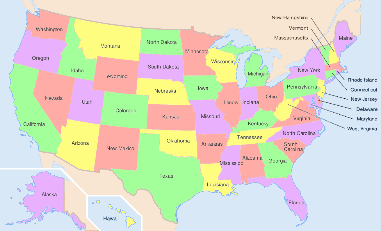
Another application of the general searches is coloring maps. The premise is that we don’t want two adjacent territories to have the coloring. These territories could be states, like in the United States map below, counties, provinces, countries, and much more.

 ^[https://commons.wikimedia.org/wiki/File:Map_of_USA_showing_state_names.png]
The following was generated for this course using the breadth first search and MyMatrixGraph class that we have implemented in this course. To create the visual rendering, the Python library NetworkX^[https://networkx.github.io/] was used. In this rendering, the starting node was Utah. If we were to start from say Alabama or Florida, we would not have a valid four coloring scheme once we got to Nevada. Since Hawaii and Alaska have no land border with any of the states, they can be any color.