Introduction

We will continue to work with graph algorithms in this module, specifically with finding minimum spanning trees (MST). MSTs have many real world applications such as:

• Electrical wiring,
• Distribution networks,
• Telecommunication networks, and
• Network routing

Suppose we were building an apartment complex and wanted to determine the most cost-effective wiring schema. Below, we have the possible construction costs for wiring apartment to apartment. Wiring vertically adjacent apartments is cheaper than wiring horizontally adjacent units and those closest to the power closet have lower costs as well.

To find the best possible solution, we would find the MST. The final wiring schema may look something like the figure below.

Determining a MST can result in lower costs and time used in many applications, especially logistics. To properly define a minimum spanning tree, we will first introduce the concept of a spanning tree.

Spanning Trees

A spanning tree for a graph is a subset of the graphs edges such that each node is visited once, no cycles are present, and there are no disconnected components.

Let’s look at this graph as an example. We have five nodes and seven edges.

Below, we have valid examples of spanning trees. In each of the examples, we visit each node and there are no cycles. Recall that a cycle is a path in which the starting node and ending node are the same.

Counterexamples

Below, we have invalid examples of spanning trees. In the left column, the examples are where all of the nodes are not connected in the same component. In the right column, the examples contain cycles. For example in the top right, we have the cycle B->C->D->E->B

Minimum Spanning Trees

Now that we have an understanding of general spanning trees, we will introduce the concept of minimum spanning trees. First let’s introduce the concept of the cost of a tree.

The cost that is associated with a tree, is the sum of its edges weights. Let’s look at this spanning tree which is from the previous page. The cost associated with this spanning tree is: 2+6+10+14=32.

Minimum Spanning Trees (MST)

A minimum spanning tree is a spanning tree that has the smallest cost. Recall the graph from the previous page.

Below on the left is a minimum spanning tree for the graph above. On the right is an example of a spanning tree, though it does not have the minimum cost.

In this small example, it is rather straightforward to find the minimum spanning tree. We can use a bit of trial and error to determine if we have the minimum spanning tree or not. However, once the graphs start to get more nodes and more edges it quickly becomes more complicated.

There are two algorithms that we will introduce to give us a methodical way of finding the minimum spanning tree. The first that we will look at is Kruskal’s algorithm and then we will look at Prim’s algorithm.

Kruskal

As graphs get larger, it is important to go about finding the MST in a methodical way. In the mid 1950’s, there was a desire to form an algorithmic approach for solving the ’traveling salesperson’ problem^[We will describe this problem in a future section of this module]. Joseph Kruskal first published this algorithm in 1956 in the Proceedings of the American Mathematical Society^[https://www.ams.org/journals/proc/1956-007-01/S0002-9939-1956-0078686-7/S0002-9939-1956-0078686-7.pdf]. The algorithms prior to this were, as Kruskal said, “unnecessarily elaborate” thus the need for a more succinct algorithm arose.

Algorithm

In his original work, Kruskal outlined three different yet similar algorithms to finding a minimum spanning tree. The Kruskal Algorithm that we use is as follows:

1. Start with only the nodes of the graph and an empty set for the edges
2. Order the edges based on weight
3. Make each node their own set
4. Go through the edges in ascending order
5. If nodes u and v are connected by the edge and they are not in the same set yet, then join the two sets and add the edge to your set of edges

Starting Graph

Resulting MST

Pseudocode

function KRUSKAL(GRAPH)
    MST = GRAPH without the edges attribute(s)
    ALLSETS = an empty list which will contain the sets
    for NODE in GRAPH NODES
        SET = a set with element NODE
        add SET to ALLSETS
    EDGES = list of GRAPH's edges
    SORTEDEDGES = EDGES sorted by edge weight, smallest to largest
    for EDGE in SORTEDEDGES
        SRC = source node of EDGE
        TAR = target node of EDGE
        SRCSET = the set from SETS in which SRC is contained
        TARSET = the set form SETS in which TAR is contained
        if SRCSET not equal TARSET
            UNIONSET = SRCSET union TARSET
            add UNIONSET to ALLSETS
            remove SRCSET from ALLSETS
            remove TARSET from ALLSETS
            add EDGE to MST as undirected edge
    return MST

Prim

The history of Prim's Algorithm is not as straight forward as Kruskal’s. While we often call it Prim's Algorithm, it was originally developed in 1930 by Vojtěch Jarník. Robert Prim later rediscovered and republished this algorithm in 1957, one year after Kruskals. To add to the naming confusion, Edsger Dijkstra also published this work again in 1959. Because of this, the algorithm can go by many names: Jarkík's Algorithm, Jarník-Prim's Algorithm, Prim-Dijkstra's Algorithm, and DJP Algorithm.

Prim cited “large-scale communication” as the motivation for this algorithm, specifically the “Bell System leased-line”^[R.C. Prim, May 8, 1957 Shortest Connection Networks And Some Generalizations https://archive.org/details/bstj36-6-1389]. Leased lines were used primarily in a commercial setting which connected business offices that were geographically distant (IE in different cities or even states). Companies would want all offices to be connected but wanted to avoid having to lay an excessive amount of wire. Below is a figure which Prim used to motivate the need for the algorithm. This image depicts the minimum spanning tree which connect each of the US continental state capitals along with Washington D.C.

Algorithm

The basis of the algorithm is to start with only the nodes of the graph, then we do the following

1. Choose a random node
2. Grow your tree by one edge, selecting the smallest edge to connect to a node that is not yet in the tree. Repeat until all the nodes have been visited

Starting Graph

Resulting MST

Info

Uniqueness

You may have noticed that the minimum spanning tree that resulted from Kruskal’s algorithm differed from Prim’s algorithm. We have displaying them both below for reference.

Kruskal	Prim

While these are different, they are both valid. The trees both have cost 16. The MST of a graph will be unique, meaning there is only one, if none of the edges of the graph have the same weight.

Pseudocode

function PRIM(GRAPH, START)
    MST = GRAPH without the edges attribute(s)
    VISITED = empty set
    add START to VISITED
    AVAILEDGES = list of edges where START is the source
    sort AVAILEDGES
    while VISITED is not all of the nodes
        SMLEDGE = smallest edge in AVAILEDGES
        SRC = source of SMLEDGE
        TAR = target of SMLEDGE
        if TAR not in VISITED
            add SMLEDGE to MST as undirected edge
            add TAR to VISITED
            add the edges where TAR is the source to AVAILEDGES
        remove SMLEDGE from AVAILEDGES
        sort AVAILEDGES
    return MST

Traveling Salesperson

While we won’t outline algorithms suited for solving the traveling salesperson problem (TSP), we will outline the premise of the problem. This problem was first posed in 1832, almost a two centuries ago, and is still quite prevalent. It is applicable to traveling routes, distribution networks, computer architecture and much more. The TSP is a seminal problem that has motivated many research breakthroughs, including Kruskals algorithm!

The motivation of the TSP is this: given a set of locations, what is the shortest path such that we can visit each location and end back where started?

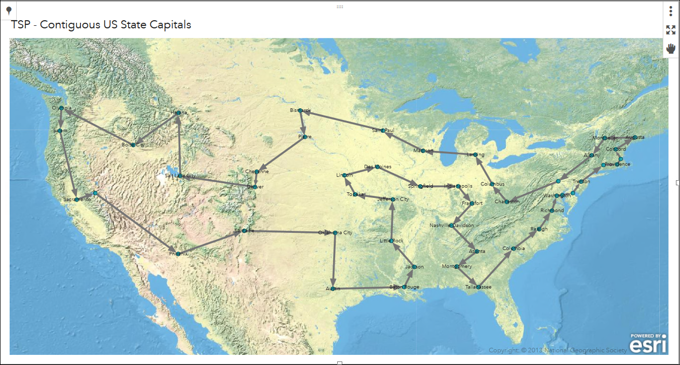
Suppose we wanted to take a roadtrip with friends to every state capital in the continental US as well as Washington D.C. To save money and time, we would want to minimize the distance that we travel. Since we are taking a roadtrip, we would want to avoid frivolous driving. For example, if we start in Sacremento, CA we would not want to end the trip in Boston, MA. The trip should start and end at the same location for efficiency.

The figure below shows the shortest trip that visits each state capital and Washington D.C. once. In this example, we can start where ever we like and will end up where we started. ^[PatriciaNeri, August 2018 https://communities.sas.com/t5/SAS-Communities-Library/What-is-the-shortest-tour-that-visits-only-once-the-48/ta-p/490231]

In this problem, it is easy to get overwhelmed by all of the possibilities. Since there are 49 cities to visit, there are over 6.2*10^60 possibilities. For reference, 10^12 is equivalent to one trillion! Thus, we need an algorithmic approach to solve this problem as opposed to a brute force method.