Subsections of Iii-Graphs
Chapter 30
Graphs: Matrix Representation
Welcome!
This page is the main page for Graphs: Matrix Representation
Subsections of Graphs: Matrix Representation
Introduction
YouTube VideoThe next data structure we will introduce is a graph.

Graphs are multidimensional data structures that can represent many different types of data. We can use graphs to represent electronic circuits and wiring, transportation routes, and networks such as the Internet or social groups.
A popular and fun use of graphs is to build connections between people such as Facebook friends or even connections between performers. One example is the parlor game Six Degrees of Kevin Bacon. Players attempt to connect Kevin Bacon to other performers through movie roles in six people or less.

For example, Laurence Fishburne and Kevin Bacon are directly connected via ‘Mystic River’. Keanu Reeves and Kevin Bacon have never performed in the same film, but Keanu Reeves and Laurence Fishburne are connected via ‘The Matrix’. Thus, Keanu and Kevin are connected via Laurence.
In this module we will discuss graphs in more detail and build our own implementation of graphs.
Terms I
YouTube VideoWe will discuss some of the basic terminology associated with graphs. Some of this vocabulary should feel familiar from the trees section; trees are a specific type of graph!
Nodes: Node is the general term for a structure which contains an item.Size: The size of a graph is the number of nodes.Capacity: The capacity of a graph is the maximum number of nodes.
Info
Nodes can be, but are not limited to the following examples: - physical locations (IE Manhattan, Topeka, Salina), - computer components (IE CPU, GPU, RAM), or - people (IE Kevin Bacon, Laurence Fishburne, Emma Stone)
Edges: Edges are the connection between two nodes. Depending on the data, edges can represent physical distance, films, cost, and much more.Adjacent: Node A and node B are said to be adjacent if there is an edge from node A to node B.Neighbors: The neighbors of a node are nodes which are adjacent to the node.
Info
Edges can be, but are not limited to: - physical distances, like the distance between cities or wiring between computer components, - cost, like bus fares, and - films, like the Six Degrees of Kevin Bacon example
Cycles: A cycle is a path where the first and last node are the only repeated nodes. More explicitly, this means that we start at node A and are able to end up back at node A.
Example
For example, we can translate the Amtrak Train Station Connections into a graph where the edges represent direct train station connections.
 ^[Generated using the Amtrak system map from 2018. This graph does not include all stations or connections.]
Within this context, we could say that Little Rock and Fort Worth are adjacent. The neighbors of San Antonio are Fort Worth, Los Angeles, and New Orleans. The Amtrak Train Graph has multiple cycles. One of these is Kansas City -> St. Louis -> Chicago -> Kansas City.
Graph Features
YouTube VideoWhile trees are a type of graph, graphs can have more functionality than trees. For example, recall that to be a single tree, there could be no disconnected pieces.
Connectedness: Graphs do not require being fully connected. There can be disconnected portions within a graph. For example, the following graph shows all of the students in a sophomore biology class. There is an edge between two student nodes if they are Facebook friends.

Graphs can also have loops. In a tree, this would be like a node being its own parent, which is not an allowable condition.
Loops: Loops are edges which connect a node to itself. These can be useful in depicting graphs that show control flow in programming. In this example, node A is connected to node B and node A is connected to itself.

Weighted Graphs
YouTube VideoA weighted graph is a graph which has weights associated with the edges. These weights quantify the relationships, so they can represent dollars, minutes, miles, and many other factors which our data may depend upon.
Weights are not limited to physical quantities; they can also be our own defined similarity in text, product types, and anything for which we can create a similarity measure for. Let’s look at concrete weights using the Amtrak example.
We are able to expand the Amtrak graph from the previous page to include approximate distances in miles between cities.
 ^[Generated using the Amtrak system map from 2018. This graph does not include all stations or connections. Distance was calculated approximately ‘as the crow flies’.]
Now that we have weights defined on our edges, we can compare paths in a different way. When we discussed trees, we just looked at the number of edges it took to get to another node. We can also determine the shortest path between nodes with respect to distance. If we wanted to travel from San Antonio to Kansas City, we may be tempted to travel San Antoinio -> Los Angeles -> Albuquerque -> Kansas City as it has the fewest stops. This trip would take us 2,531 miles (1201+640+690). With the edge weights in mind, a much better route would be San Antonio -> Fort Worth -> Little Rock -> St. Louis -> Kansas City with a total of 1,089 miles(238+320+293+238) traveled.
Directed Graphs
YouTube VideoA directed graph is a graph that has a direction associated with each edge. For example, trees are a directed graph. The edge orientation will imply a fixed direction that we can move about nodes. As with trees, the flat end of the arrow will represent the origin and the arrowhead will represent the destination. If an edge has no arrowheads, then it is assumed that we can traverse both directions.
In the following graph, we have an example distribution network where each store ends up with 5 units in its possession. For example, nine units go from the distribution center to Store A. The distribution center will never receive product from stores as it has no incoming edges.

Unlike trees, directed graphs can have nodes with multiple incoming edges. We can see an example of this at Store B. The distribution center and Store A both send units to Store B.
Info
In directed graphs, we must be cautious on how we define adjacent. For the following, we would say that the source is adjacent to the target. However, the target is not adjacent to the source.

Formally, node A and node B are said to be adjacent if there is an edge from node A to node B.
When discussing directed graphs, we must also talk about undirected graphs. An undirected graph is a graph in which none of the edges have an orientation. If there is at least one directed edge, then it is considered a directed graph.
Undirected Edge: An undirected edge is an edge which has no defined orientation (IE no arrowheads) which implies that we can traverse in either direction. If node A and node B are connected via an undirected edge then we say node A is adjacent to node B and node B is adjacent to node A.
Info
For the following undirected edge, we would say that the source is adjacent to the target and the target is adjacent to the source.

Info
Graph types and appearances can vary wildly. We are not limited to just weighted/unweighted or directed/undirected. We can also have combinations of weighted and directed.
Example
In the following graph, we have an example of a weighted and directed map. This map represents a zoo train where each node represents a station and each edge is a part of the track. Zoo guests can get on and off wherever they desire.
This graph is weighted as guests must pay the associated fee for each part of the track. Our example train also has a one way direction in most cases. The exception to this is the entrance/exit to the aquarium, this part of the track can go either direction.
In this graph, we also have a couple of loops. This would allow for zoo-guests to ride the train around an expansive exhibit such as the elephants or giraffes.
One possible way to tour the zoo for a guest starting at the entrance could be: aquarium, primates, big cats, antelope, giraffes, loop around the giraffes, elephants, aquarium, then exit. Their total payment for just the train would be $14.

Matrix Representation
YouTube VideoThe first way that we can represent graphs is as matrices. In a matrix representation of a graph, we will have an array with all the nodes and a matrix to depict the edges. The matrix that depicts the edges is called the adjacency matrix.
To build the adjacency matrix, we go through the nodes and edges. If there is an edge with weight w going from i to j, then we put w in the (i,j) spot in our adjacency matrix. If there is no edge from i to j then we put infinity in the spot (i,j). Let’s look at some examples.
Info
An edge that starts at source and ends at target will result in an entry at (source,target) in the adjacency matrix.
Info
For an unweighted graph, we treat the weights as 1 for all edges in our adjacency matrix.
For an undirected edge between nodes i and j, we put an edge from i to j and an edge from j to i.
Example 1
Suppose that we have the following graph:

Across the top of the following, we have the array of nodes. This give us the index at which each node is located. For example, node A is in spot 1, node B is in spot 2, node C is in spot 3 and so on.
Below that we have the adjacency matrix. For the directed edge with weight 2 that goes from node B to node C, we have the value 2 at (2,3) in the adjacency matrix as B has index 2 and C has index 3. For the directed edge with weight 4 that goes from node A to node F, we have the value 4 at (1,6) in the adjacency matrix as A has index 1 and F has index 6.
Since there is no edge that connects from node A to node B, we have infinity in (1,2).

Example 2
Now suppose we have this graph. We now have some loops present.

For example, we have a loop on node E with weight 12 so we will put the value 12 in spot (5,5) as E has index 5.

Example 3
Now suppose we have this graph which is undirected and unweighted.

Since this graph is unweighted, we will treat all edges as though they have weight equal to one. Since this graph is undirected, each edge will essentially show up twice.
For example, for the edge that connects nodes A and B, we will have an entry in our adjacency matrix at (1,2) and (2,1).

UML
YouTube Video
Attributes
nodes: This will keep track of the nodes which are in our graph as well as the node values. The nodes can have any type of value such as numbers, characters, and even other data structures.edges: This will keep track of the edges which are in our graph.size: This will keep track of the number of nodes that are active in our graph.
Upon initialization, we will initialize nodes to be an empty array of size capacity, edges to be an empty two-dimensional array with dimensions capacity by capacity and size to be zero as we start with no actual nodes.
Getters
get nodes: returns a list of the nodes with their respective indexes
function GETNODES()
    LIST = []
    for NODE in NODES
        if NODE has a VALUE
            append (VALUE, INDEX) to LIST
    return LIST
get edges: returns a list of the edges in the format (source, target, weight)
function GETEDGES()
    LIST = []
    for ROW in EDGES
        for COL in ROW
            VALUE = entry at (ROW,COL)
            if VALUE is not infinity
                    append (ROW,COL,VALUE) to LIST
return LIST-
get node: returns the node with the given index. If the index is within the possible range, then we return the value of that node. -
find node: returns the index of the given node. We iterate through our nodes and if we find that value, then we return the index. Otherwise, return-1. -
get edge: returns the weight of the edge between the given indexes of the source node and target node. If one or both of the indexes are out of range, then we should return infinity. -
get capacity: returns the maximum number of nodes we are allowed to have. Upon initialization, we will have a fixed number of possible nodes in our node array. We can simply return the size of this array. -
get size: returns the size attribute. -
get number of edges: returns the number of edges currently in the graph. We will iterate through our edges and return the number of entries that were not infinity. -
get neighbors: returns the neighbors of the given node. We will access our row adjacency matrix that corresponds to the node and return the indexes and values of those entries which are not infinity.
function GETNEIGHBORS(IDX)
    if IDX in range of NODES length
        LIST = []
        ROW = the IDX-th row of EDGES
        for J in range  0 to ROW length
            VALUE = J-th entry of ROW
            if VALUE is not infinity
                    append (J,VALUE) to LIST
        return LIST
Node and Edge Functions
YouTube Videoadd node: will add a node to the graph with the given value if our graph still has room. Procedurally, we will try to put the node in the first empty place we find. To do this, we start withIDXequal to negative one then loop through all of the indexes of the graphsnodesattribute. At each index, we check if that entry is equal to the value we are trying to add. This will check if the value is already in our graph. If there is nothing in that entry and theIDXvariable is still negative one, then we will setIDXequal to that index. We continue looping through thenodesattribute until we reach the end. It is possible that there is more than one open space in thenodesattribute. Thus, by checking ifIDXis still negative one we can make sure to putvaluein the first empty spot. Once we finish going throughnodeswe check to see if we ever found an open spot. IfIDXis still negative one, this would indicate that there was no room. Otherwise, we putvalueintonodesat spotIDXand increment the size.
function ADDNODE(VALUE)
    IDX = -1
    for NODE in NODES
        if NODE is VALUE
            return NODE's index
        if NODE has no entry and IDX is -1
            IDX = NODE's index
    if IDX is not -1
        add VALUE to NODES at position IDX
        increment SIZE
    return IDX
remove node: will remove a node to the graph with the given value if our graph has the node. We will set the node to be empty and remove any edges that may be attached to it.
function REMOVENODE(IDX)
    if IDX is in the range of our indexes
        if NODES at position IDX is not empty
            set NODES at IDX to be empty
            decrement SIZE by one
            for J in node indexes
                set EDGES (J,IDX) equal to infinity
                set EDGES (IDX,J) equal to infinity
            return true
        else
            return false
    else
        return false
add edge: will add an edge with the given weight which goes from the source node to the target node
function ADDEDGE(SOURCE, TARGET, WEIGHT)
    if SOURCE and TARGET are both in the range of our node indexes
        set EDGES(SOURCE, TARGET) equal to WEIGHT
        return true
    else
        return false
remove edge: will remove the edge which goes from the source node to the target node
function REMOVEEDGE(SOURCE, TARGET)
    if SOURCE and TARGET are both in the range of our node indexes
        if EDGES(SOURCE, TARGET) is not equal to infinity
            set EDGES(SOURCE, TARGET) equal to infinity
            return true
        else
            return false
    else
        return false
add undirected edge: will add two edges with the given weight between the two given nodes
function ADDUNDIRECTEDEDGE(NODE1, NODE2, WEIGHT)
    RES = ADDEDGE(NODE1, NODE2, WEIGHT)
    RES = RES and ADDEDGE(NODE2, NODE1, WEIGHT)
    return RES
remove undirected edge: will remove two edges between the two given nodes. We can utilize the remove edge function on ‘NODE1’ to ‘NODE2’ and then on ‘NODE2’ to ‘NODE1’.
function REMOVEUNDIRECTEDEDGE(NODE1, NODE2)
    RES = REMOVEEDGE(NODE1, NODE2)
    RES = RES and REMOVEEDGE(NODE2, NODE1)
    return RES
Summary
In this module, we have introduced the graph data structure. We also looked at how we would implement a graph using a matrix representation. We introduced the following new concepts in this module:
-
Directed Graphs: A directed graph is a graph that has a direction associated with each edge. The flat end of the arrow will represent the origin and the arrowhead will represent the destination. If an edge has no arrowheads, then it is assumed that we can traverse both directions. -
Edges: Edges are the connection between two nodes. Depending on the data, edges can represent physical distance, films, cost, and much more.Adjacent: Node A and node B are said to be adjacent if there is an edge from node A to node B.Neighbors: The neighbors of a node are nodes which are adjacent to the node.Undirected Edge: An undirected edge is an edge which has no defined orientation (IE no arrowheads). If node A and node B are connected via an undirected edge then we say node A is adjacent to node B and node B is adjacent to node A.
-
Loops: Loops are edges which connect a node to itself. -
Nodes: Node is the general term for a structure which contains an item.Size: The size of a graph is the number of nodes.Capacity: The capacity of a graph is the maximum number of nodes.
-
Weighted Graphs: A weighted graph is a graph which has weights associated with the edges. These weights will quantify the relationships so they can represent dollars, minutes, miles, and many other factors which our data may depend on.
In the next module, we will look at a list implementation of graphs and when we might use one implementation over the other.
Chapter 35
Graphs: List Representation
Welcome!
This page is the main page for Graphs: List Representation
Subsections of Graphs: List Representation
Introduction
YouTube VideoIn the previous module, we introduced graphs and a matrix-based implementation. For this module, we will continue working with graphs and change our implementation to lists.
Why Another Implementation?
When using graphs, a lot of situational variation can occur. Some graphs can have a few nodes with many edges, many nodes with few edges, and so on. When we use the matrix implementation, we initialize a matrix with the number of columns and rows equal to the number of nodes. For example, if we have a graph with 20 nodes, our adjacency matrix would have 20 rows and 20 columns, resulting in 400 potential entries.
First let’s look at the implementation and then we will discuss when one may be better than the other.
List Representation
YouTube VideoIn the matrix representation, we had an array of the node items. In the list representation, we will have an array of node objects. Each node object will keep track of the node item, the node index, and the outgoing edges.

The item can be any object and the index will be a value within our capacity. The edges will be a list of pairs where the first entry is the index of the target node and the second entry is the weight of the edge.
Since each node will track its neighbors, it is important that we are consistent in our indexing of nodes. If our nodes were to get out of order, then our edges would as well.
Example 1
Consider the following graph which we saw in the matrix representation.
The following list of nodes depicts the graph above. We can see that each node object has the item and index.
If we look closer at the edges of the node with item A and index 1, we see that the set of edges is equal to [(4, 3.0), (6, 4.0)]. This corresponds to the fact that there are two edges with the source as node 1. The first ordered pair, (4, 3.0), means that there is an edge with source node 1 (A) and target node 4 (D) that has weight 3. We can confirm that in our graph we do have an edge from A to D with weight 3.

Example 2
The following includes a couple of examples of loops within our graph.
We have loops on nodes D, E, and F in our graph. Recall that a loop is an edge where the source and target are the same. For example, we have an edge with source D and target D that has weight 12. We see this in our list representation in the node object with item D and index 4, where we have the entry (4,12.0) in the edges.

Dense VS Sparse
YouTube VideoWhen considering which implementation to use, we need to consider the connectivity in our graph. The terms that we use to describe the connectedness are dense and sparse.
Dense Graph: A dense graph is a graph in which there is a large number of edges. Typically in a dense graph, the number of edges is close to the maximum number of edges.Sparse Graph: A sparse graph is a graph in which there is a small number of edges. In this case the number of edges is considerably less than the maximum number of edges.
Info
Intuitively, we can think of dense and sparse in terms of populations. For example, if 100 people lived in a city block, we can consider that to be densely populated. If 100 people lived in 100 square miles we can consider that to be sparsely populated.
Let’s look at some motivating examples to get an idea of how the different structures will handle these cases.
Dense
The following is a dense graph. In this case, our graph does have the maximum number of edges. This means that every node is connected to every other node including itself.


Sparse
The following is a sparse graph.


List or Matrix?
For dense graphs, the matrix representation will have better qualities as we are already setting aside space for the maximum number of edges. Sparse graphs are better represented in the list representation.
When we initialize the matrix implementation, we initialize the nodes attribute to have dimension equal to the capacity of the graph. The edges attribute is initialized to be a square matrix with dimension equal to capacity by capacity. Thus, if we have a sparse matrix, we are representing a lot of non-existent edges.
When we initialize the list implementation, we just have the nodes attribute which has dimension equal to the capacity and each node tracks its own edges. If we have a dense matrix and we are searching for an edge, we must loop through each edge from the target node to see if the edge exists. In the matrix representation, we can access that edge directly.
Info
If the proportion of edges to the maximum number of edges is greater than 1/64, then the matrix representation is better in terms of space.
UML - Graph Node
YouTube VideoIn this representation, we will have an array of graph node objects. We will first cover the UML for the graph node objects and then discuss the graph functions and attributes.

Attributes
item: the value that the node contains.index: the index of the node.edges: ordered pairs(e, w)where this node is the source,eis the target node index, andwis the weight of the edge as a double.
We will initialize a graph node with the given item and the given index. We initialize the edges attribute to be an empty list.
Getters
-
get item: Returns the graph node’s item. -
get index: Returns the graph node’s index. -
get edges: Returns the graph node’s edges. -
get edge: From the source node, we will call the get edge function with the index of the target node as input. This will return the edge weight.
function GETEDGE(TARINDEX)
    for EDGE in nodes EDGES
        if the first element in EDGE is TARINDEX
            return the second element in EDGE
    return infinity
Edge Functions
Info
Working with the edges in our graph becomes slightly more complicated in the list representation. Previously, we were able to go right to the entry in our adjacency matrix and update it. Since each node keeps track of its own edges in no particular order, we must loop through each entry of the edges attribute to find a potential edge.
add edge: From the source node, we will call the add edge function with the target node as input as well as the weight. First, we will attempt to remove the edge. We need to do this as we do not want duplicate edges in our graph. Then we will add the ordered pair to the edges attribute.
function ADDEDGE(TARINDEX, WEIGHT)
    call REMOVEEDGE(TARINDEX) on this node
    append (TARINDEX, WEIGHT) to this nodes EDGES
remove edge: From the source node, we will call the remove edge function with the target node as input. This will return true if it was successful and false if not.
function REMOVEEDGE(TARINDEX)
    for EDGE in nodes EDGES
        if the first element in EDGE is TARINDEX
            remove EDGE from EDGES
            return true
    return false
UML - Graph
YouTube Video
Attributes
nodes: This will keep track of the nodes which are in our graph as well as the node values. The nodes can have any type of value such as numbers, characters, and even other data structures.size: This will keep track of the number of nodes that are active in our graph.
Upon initialization, we will initialize nodes to be an empty array with dimension capacity and size to be zero as we start with no actual nodes.
Getters
get nodes: returns a list of the nodes with their respective indexes. This will be the same logic from our matrix graph.
function GETNODES()
    LIST = []
    for NODE in NODES
        if NODE has a VALUE
            append (VALUE, INDEX) to LIST
    return LIST
get edges: returns a list of the edges in the format (source, target, weight).
function GETEDGES()
    LIST = []
    for NODE in NODES
        if NODE is not empty
            for EDGE in NODE EDGES
                TAR = first entry of EDGE
                WEIGHT = second entry of EDGE
                append (NODE,TAR,WEIGHT) to LIST
return LIST-
get node: returns the node with the given index. If the index is within the possible range, then we return the value of that node. This will be the same logic from our matrix graph. -
find node: returns the index of the given node. We iterate through our nodes and if we find that value, then we return the index. Otherwise, return-1. This will be the same logic from our matrix graph. -
get edge: returns the weight of the edge between the given indexes of the source node and target node. If one or both of the indexes are out of range, then we should return infinity. From the source node object, we will call the graph node get edge function on the target index.
function GETEDGE(SRC,TAR)
    if SRC and TAR are between 0 and capacity
        SRCNODE = the node at index SRC of the NODES attribute
        WEIGHT = call the graph node GETEDGE from SRCNODE on TAR
        return WEIGHT
    else
return infinity-
get capacity: returns the maximum number of nodes we are allowed to have. Upon initialization, we will have a fixed number of possible nodes in our node array. We can simply return the size of this array. This will be the same logic from our matrix graph. -
get size: returns the size attribute. This will be the same logic from our matrix graph. -
get number of edges: returns the number of edges currently in the graph.
function NUMBEROFEDGES()
    COUNT = 0
    for NODE in NODES
        if NODE is not empty
            for EDGE in NODE EDGES
                increment COUNT by one
    return COUNT
get neighbors: returns the neighbors of the given node. We will access our row adjacency matrix that corresponds to the node and return the indexes and values of those entries which are not infinity.
function GETNEIGHBORS(IDX)
    SRCNODE = the node at index IDX of the NODES attribute
    if SRCNODE is not empty
        return SRCNODE's edges
    else
        return nothing
Node and Edge Functions
add node: will add a node to the graph with the given value if our graph still has room. Finding a location for the node will be the same procedure as the matrix graph. If we find an open spot to add the node, we will instantiate a new graph node and insert it into thenodesattribute.
function ADDNODE(VALUE)
    IDX = -1
    for NODE in NODES
        if NODE is VALUE
            return NODE's index
        if NODE has no entry and IDX is -1
            IDX = NODE's index
    if IDX is not -1
        NEWNODE = graph node with VALUE and IDX for input
        add NEWNODE to NODES at position IDX
        increment SIZE
    return IDX
remove node: will remove a node to the graph with the given value if our graph has the node. We will set the node to be empty. When we set the node to be empty, we clear all of the outgoing edges, so we just need to loop through the other nodes removing any possible incoming edges.
function REMOVENODE(IDX)
    if IDX is in the range of our indexes
        if NODES at position IDX is not empty
            set NODES at IDX to be empty
            decrement SIZE by one
            for NODE in NODES
                if NODE has no entry
                    from NODE call the graph node REMOVEEDGE function on IDX
            return true
        else
            return false
    else
        return false
add edge: will add an edge with the given weight which goes from the source node to the target node
function ADDEDGE(SRC, TAR, WEIGHT)
    if SOURCE and TARGET are both in the range of our node indexes
        SRCNODE = the node at index SRC of the NODES attribute
        if SRCNODE is not empty
            from SRCNODE call the graph node ADDEDGE with TAR and WEIGHT as input
            return true
        else
            return false
    else
        return false
remove edge: will remove the edge which goes from the source node to the target node
function REMOVEEDGE(SOURCE, TARGET)
    if SOURCE and TARGET are both in the range of our node indexes
        SRCNODE = the node at index SRC of the NODES attribute
        if SRCNODE has no entry
            RET = SRCNODE call the graph node REMOVEEDGE with TAR as input
            return RET
        else
            return false
    else
        return false
add undirected edge: will add two edges with the given weight between the two given nodes
function ADDUNDIRECTEDEDGE(NODE1, NODE2, WEIGHT)
    RES = ADDEDGE(NODE1, NODE2, WEIGHT)
    RES = RES and ADDEDGE(NODE2, NODE1, WEIGHT)
    return RES
remove undirected edge: will remove two edges between the two given nodes.
function REMOVEUNDIRECTEDEDGE(NODE1, NODE2)
    RES = REMOVEEDGE(NODE1, NODE2)
    RES = RES and REMOVEEDGE(NODE2, NODE1)
    return RES
Summary
In this module, we introduced a new way to store the graph data structure. Thus, we now have two ways to work with graphs, in lists and in matrices:
List Representation
Matrix Representation
While these methods show the same information, there are cases when one way may be more desirable than the other.
We discussed how a sparse graph is better suited for a list representation and a dense graph is better suited for a matrix representation. We also touched on how working with the edges in a list representation can add complexity to our edge functions. If we are needing to access edge weights or update edges frequently, a matrix representation would be a good choice – especially if we have a lot of nodes.
Chapter 40
Graphs: Searching and Traversing
Welcome!
This page is the main page for Graphs: Searching and Traversing
Subsections of Graphs: Searching and Traversing
Introduction
YouTube VideoIn the previous modules, we have introduced graphs and two implementations. This module will cover the traversals through graphs as well as path search techniques.
Motivation
As we have discussed previously, graphs can have many applications. Based on that, there are many things that we may want to infer from graphs. For example, if we have a graph that depicts a railroad or electrical network, we could determine what maximum flow of the network. The standard approach for this task is the Ford-Fulkerson Algorithm. In short, given a graph with edge weights that represent capacities the algorithm will determine the maximum flow throughout the graph.
From the matrix graph module, we used the following distribution network as an example.
Conceptually, we would want to determine the maximum number of units that could leave the distribution center without having excess laying around stores. Using the maximum flow algorithm, we would determine that the maximum number of units would be 15.

The driving force in the Ford-Fulkerson algorithm, as well as other maximum flow algorithms, is the ability to find a path from a source to a target. Specifically, these algorithms use breadth first and depth first searches to discover possible paths.
Searches
To get to introducing the searches, we will first discuss the basis of them. Those are the depth first traversal and the breadth first traversal. We will outline the premise of these traversals and then discuss how we can modify their algorithms for various tasks, such as path searches.
We can perform these traversals on any type of graph. Conceptually, it will help to have a tree-like structure in mind to differentiate between depth first and breadth first.

Depth First
First we will discuss Depth First Traversal. We can define the depth first traversal in two ways, iteratively or recursively. For this course, we will define it iteratively.
In the iterative algorithm, we will initialize an empty stack and an empty set. The stack will determine which node we search next and the set will track which nodes we have already searched.
Info
Recall that a stack is a ‘Last In First Out’ (LIFO) structure. Based on this, the depth first traversal will traverse a nodes descendants before its siblings.
To do the traversal, we must pick a starting node; this can be an arbitrary node in our graph. If we were doing the traversal on a tree, we would typically select the root at a starting point. We start a while loop to go through the stack which we will be pushing and popping from. We get the top element of the stack, if the node has not been visited yet then we will add it to the set to note that we have now visited it. Then we get the neighbors of the node and put them onto the stack and continue the process until the stack is empty.
function DEPTHFIRST(GRAPH,SRC)
    STACK = empty array
    DISCOVERED = empty set
    append SRC to STACK
    while STACK is not empty
        CURR = top of the stack
        if CURR not in DISCOVERED
            add CURR to DISCOVERED
            NEIGHS = neighbors of CURR
            for EDGE in NEIGHS
                NODE = first entry in EDGE
                append NODE to STACK
Since the order of the neighbors is not guaranteed, the traversal on the same graph with the same starting node can find nodes in different orders.
Breadth First
YouTube VideoWe can also perform a breadth first traversal either iteratively or recursively. As with the depth first traversal, we will define it iteratively.
In the iterative algorithm, we initialize an empty queue and an empty set. Like depth first traversal, the set will track which nodes we have discovered. We now use a queue to track which node we will search next.
Info
Recall that a queue is a ‘First In First Out’ (FIFO) structure. Based on this, the breadth first traversal will traverse a nodes siblings before its descendants.
Again, we must pick a starting node; this can be an arbitrary node in our graph. We add the starting node to our queue and the set of discovered nodes. We start a while loop to go through the queue which we will be enqueue and dequeue from. We get the first element of the queue, then get the neighbors of the current node. We loop through each edge adding the neighbor to the discovered set and the queue if it has not already been discovered. We continue this process until the queue is empty.
function BREADTHFIRST(GRAPH,SRC)
    QUEUE = empty queue
    DISCOVERED = empty set
    add SRC to DISCOVERED
    add SRC to QUEUE
    while QUEUE is not empty
        CURR = first element in QUEUE
        NEIGHS = neighbors of CURR
        for EDGE in NEIGHS
            NODE = first entry in EDGE
            if NODE is not in DISCOVERED
                add NODE to DISCOVERED
                append NODE to QUEUE
Info
It is important to remember in these implementations that a stack is used for depth first and a queue is used for a breadth first. The stack, being a LIFO structure, will proceed with the newest entry which will put us farther away from the source. The queue, being a FIFO structure, will proceed with oldest entry which will focus the algorithm more on the adjacent nodes. If we were to use say a queue for a depth first search, we would be traversing neighbors before descendants.
Limitations
YouTube VideoWhen introducing graphs, we discussed how the components of a graph didn’t have to all be connected. If our goal is to visit each node, like in the searches, then we will need to perform the search from every node.
For example, the graph below has two separate components. Lets walk through which nodes we will discover by calling the traversals from each node.

| Start | Visited (in alphabetical order) |
|---|---|
| A | {A, D, H} |
| B | {B, E, H, I} |
| C | {C} |
| D | {D} |
| E | {E, H, I} |
| F | {C, F} |
| G | {C, G} |
| H | {H} |
| I | {I} |
| J | {C, F, G, J} |
In this example, we would need to call either traversal on nodes A, B and J in order to visit all of the nodes.
Finding a Path
YouTube VideoAn important application for these traversals is the ability to find a path between two nodes. This has many applications in railroad networks as well as electrical wiring. With some modifications to the traversals, we can determine if electricity can flow from a source to a target. We will modify depth first and breadth first traversals in similar ways.
Info
There are three cases that can happen when we search for a path between nodes:
- No Path: will return nothing
- One Path: will return the path
- Multiple Paths: will return A path
With these searches, we are not guaranteed to return the same path if there are multiple paths.
We will call these Depth First Search (DFS) and Breadth First Search (BFS). In both traversals, we have added the following extra lines: 4, 9-16, and 22 through the end.
First, we have the addition of PARENT_MAP which will be a dictionary to keep track of how we get from one node to another. We will use the convention of having the key be the child and the value be the parent. While we use the terms child and parent, this is not exclusive to trees.
The ending portion starting at line 22, will add entries to our dictionary. If we haven’t already found an edge to NODE, then we will add the edge that we are currently on.
The other addition is the block of code from line 9 to 16. We will enter this if block if the node that we are currently at is the target. This means that we have finally found a path from the source node to the target node. The process in this segment of code will backtrack through the path and build the path.
Depth First Search (DFS)
1. function DEPTHFIRSTSEARCH(GRAPH,SRC,TAR)
2.     STACK = empty array
3.     DISCOVERED = empty set
4.     PARENT_MAP = empty dictionary
5.     append SRC to STACK
6.     while STACK is not empty
7.         CURR = top of the stack
8.         if CURR not in DISCOVERED
9.             if CURR is TAR
10.                 PATH = empty array
11.                 TRACE = TAR
12.                 while TRACE is not SRC
13.                     append TRACE to PATH
14.                     set TRACE equal to PARENT_MAP[TRACE]
15.                 reverse the order of PATH
16.                 return PATH
17.            add CURR to DISCOVERED
18.            NEIGHS = neighbors of CURR
19.            for EDGE in NEIGHS
20.                NODE = first entry in EDGE
21.                append NODE to STACK
22.                if PARENT_MAP does not have key NODE
23.                    in the PARENT_MAP dictionary set key NODE with value CURR
24.    return nothing
DFS Example
Breadth First Search (BFS)
1. function BREADTHFIRSTSEARCH(GRAPH,SRC,TAR)
2.     QUEUE = empty queue
3.     DISCOVERED = empty set
4.     PARENT_MAP = empty dictionary
5.     add SRC to DISCOVERED
6.     add SRC to QUEUE
7.     while QUEUE is not empty
8.         CURR = first element in QUEUE
9.         if CURR is TAR
10.            PATH = empty list
11.            TRACE = TAR
12.            while TRACE is not SRC
13.                    append TRACE to PATH
14.                    set TRACE equal to PARENT_MAP[TRACE]
15.                reverse the order of PATH
16.                return PATH
17.        NEIGHS = neighbors of CURR
18.        for EDGE in NEIGHS
19.            NODE = first entry in EDGE
20.            if NODE is not in DISCOVERED
21.                add NODE to DISCOVERED
22.                if PARENT_MAP does not have key NODE
23.                    in the PARENT_MAP dictionary set key NODE with value CURR
24.                append NODE to QUEUE
25.    return nothing
BFS Example
In Practice
Traveling
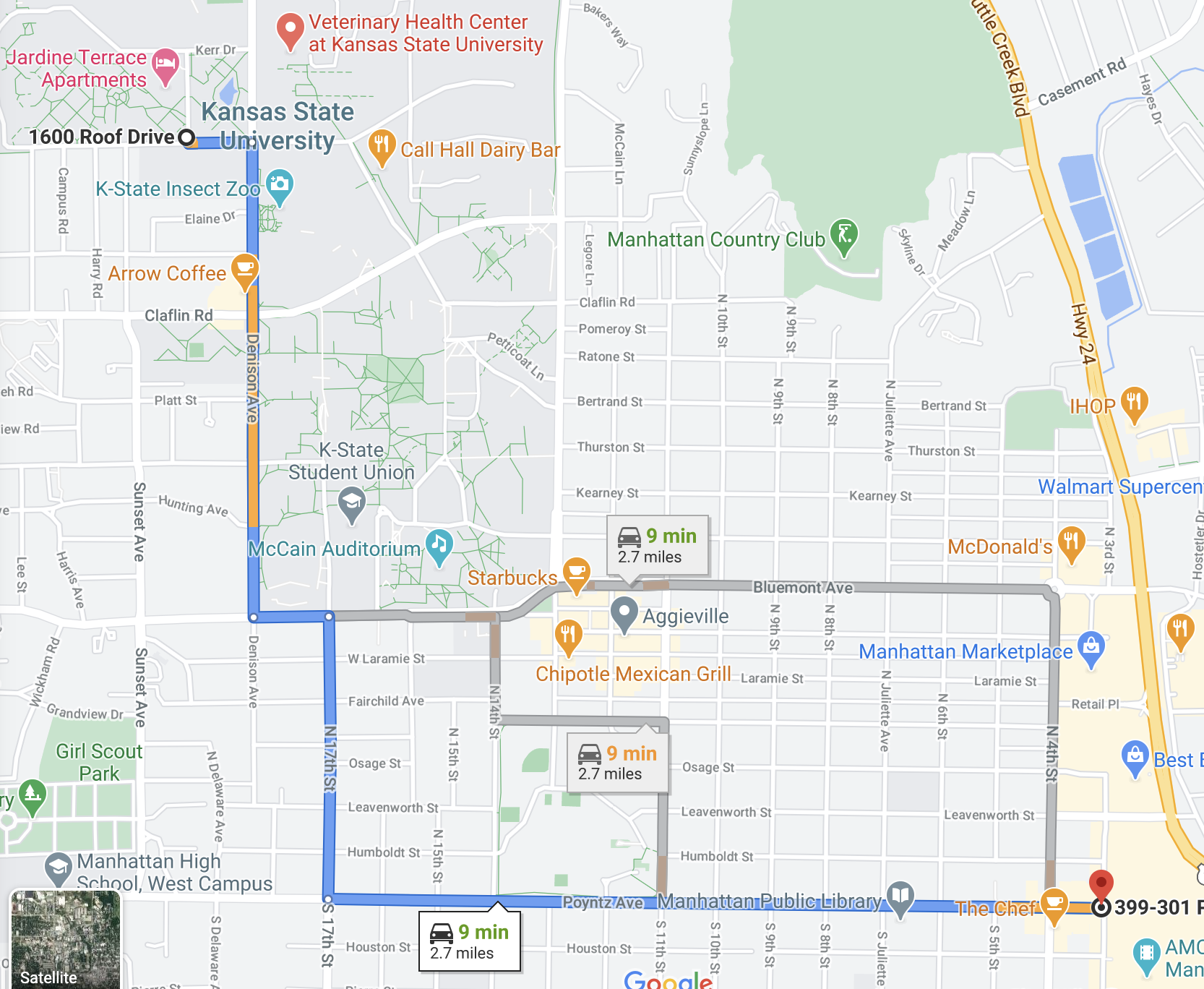
Finding a path in a graph is a very common application in many fields. One application that we benefit from in our day to day lives is traveling. Programs like Google Maps calculate various paths from point A to point B.
 ^[google.com/maps]
In the context of graph data structures, we can think of each intersection as a node and each road as an edge. Google Maps, however, tracks more features of edges than we have discussed. Not only do they track the distance between intersections, they also track time, tolls, construction, road surface and much more. In the next module, we will discuss more details of how we can find the shortest path.
Map Coloring
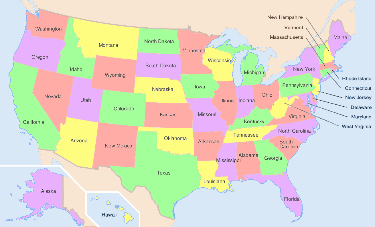
Another application of the general searches is coloring maps. The premise is that we don’t want two adjacent territories to have the coloring. These territories could be states, like in the United States map below, counties, provinces, countries, and much more.
 ^[https://commons.wikimedia.org/wiki/File:Map_of_USA_showing_state_names.png]
The following was generated for this course using the breadth first search and MyMatrixGraph class that we have implemented in this course. To create the visual rendering, the Python library NetworkX^[https://networkx.github.io/] was used. In this rendering, the starting node was Utah. If we were to start from say Alabama or Florida, we would not have a valid four coloring scheme once we got to Nevada. Since Hawaii and Alaska have no land border with any of the states, they can be any color.
Chapter 45
Graphs: Minimum Spanning Trees
Welcome!
This page is the main page for Graphs: Minimum Spanning Trees
Subsections of Graphs: Minimum Spanning Trees
Introduction
YouTube VideoWe will continue to work with graph algorithms in this module, specifically with finding minimum spanning trees (MST). MSTs have many real world applications such as:
- Electrical wiring,
- Distribution networks,
- Telecommunication networks, and
- Network routing
Suppose we were building an apartment complex and wanted to determine the most cost-effective wiring schema. Below, we have the possible construction costs for wiring apartment to apartment. Wiring vertically adjacent apartments is cheaper than wiring horizontally adjacent units and those closest to the power closet have lower costs as well.

To find the best possible solution, we would find the MST. The final wiring schema may look something like the figure below.

Determining a MST can result in lower costs and time used in many applications, especially logistics. To properly define a minimum spanning tree, we will first introduce the concept of a spanning tree.
Spanning Trees
A spanning tree for a graph is a subset of the graphs edges such that each node is visited once, no cycles are present, and there are no disconnected components.
Let’s look at this graph as an example. We have five nodes and seven edges.

Below, we have valid examples of spanning trees. In each of the examples, we visit each node and there are no cycles. Recall that a cycle is a path in which the starting node and ending node are the same.

Info
To be a spanning tree of a graph, it must:
- span the graph, meaning all nodes must be visited, and
- be a tree, meaning there are no cycles and no disconnected components.
Further, we can imagine selecting a node in a spanning tree as the root and letting gravity take effect. This gives us a visual motivation as to why they are called spanning trees. In these examples, we have selected node A for the root for each of the spanning trees above.

Counterexamples
Below, we have invalid examples of spanning trees. In the left column, the examples are where all of the nodes are not connected in the same component. In the right column, the examples contain cycles. For example in the top right, we have the cycle B->C->D->E->B

Minimum Spanning Trees
YouTube VideoNow that we have an understanding of general spanning trees, we will introduce the concept of minimum spanning trees. First let’s introduce the concept of the cost of a tree.
The cost that is associated with a tree, is the sum of its edges weights. Let’s look at this spanning tree which is from the previous page. The cost associated with this spanning tree is: 2+6+10+14=32.

Minimum Spanning Trees (MST)
A minimum spanning tree is a spanning tree that has the smallest cost. Recall the graph from the previous page.
Below on the left is a minimum spanning tree for the graph above. On the right is an example of a spanning tree, though it does not have the minimum cost.

In this small example, it is rather straightforward to find the minimum spanning tree. We can use a bit of trial and error to determine if we have the minimum spanning tree or not. However, once the graphs start to get more nodes and more edges it quickly becomes more complicated.

There are two algorithms that we will introduce to give us a methodical way of finding the minimum spanning tree. The first that we will look at is Kruskal’s algorithm and then we will look at Prim’s algorithm.
Kruskal
YouTube VideoAs graphs get larger, it is important to go about finding the MST in a methodical way. In the mid 1950’s, there was a desire to form an algorithmic approach for solving the ’traveling salesperson’ problem^[We will describe this problem in a future section of this module]. Joseph Kruskal first published this algorithm in 1956 in the Proceedings of the American Mathematical Society^[https://www.ams.org/journals/proc/1956-007-01/S0002-9939-1956-0078686-7/S0002-9939-1956-0078686-7.pdf]. The algorithms prior to this were, as Kruskal said, “unnecessarily elaborate” thus the need for a more succinct algorithm arose.
Algorithm
In his original work, Kruskal outlined three different yet similar algorithms to finding a minimum spanning tree. The Kruskal Algorithm that we use is as follows:
- Start with only the nodes of the graph and an empty set for the edges
- Order the edges based on weight
- Make each node their own set
- Go through the edges in ascending order
- If nodes
uandvare connected by the edge and they are not in the same set yet, then join the two sets and add the edge to your set of edges
Starting Graph

Resulting MST

Pseudocode
function KRUSKAL(GRAPH)
    MST = GRAPH without the edges attribute(s)
    ALLSETS = an empty list which will contain the sets
    for NODE in GRAPH NODES
        SET = a set with element NODE
        add SET to ALLSETS
    EDGES = list of GRAPH's edges
    SORTEDEDGES = EDGES sorted by edge weight, smallest to largest
    for EDGE in SORTEDEDGES
        SRC = source node of EDGE
        TAR = target node of EDGE
        SRCSET = the set from SETS in which SRC is contained
        TARSET = the set form SETS in which TAR is contained
        if SRCSET not equal TARSET
            UNIONSET = SRCSET union TARSET
            add UNIONSET to ALLSETS
            remove SRCSET from ALLSETS
            remove TARSET from ALLSETS
            add EDGE to MST as undirected edge
    return MST
Prim
YouTube VideoThe history of Prim's Algorithm is not as straight forward as Kruskal’s. While we often call it Prim's Algorithm, it was originally developed in 1930 by Vojtěch Jarník. Robert Prim later rediscovered and republished this algorithm in 1957, one year after Kruskals. To add to the naming confusion, Edsger Dijkstra also published this work again in 1959. Because of this, the algorithm can go by many names: Jarkík's Algorithm, Jarník-Prim's Algorithm, Prim-Dijkstra's Algorithm, and DJP Algorithm.
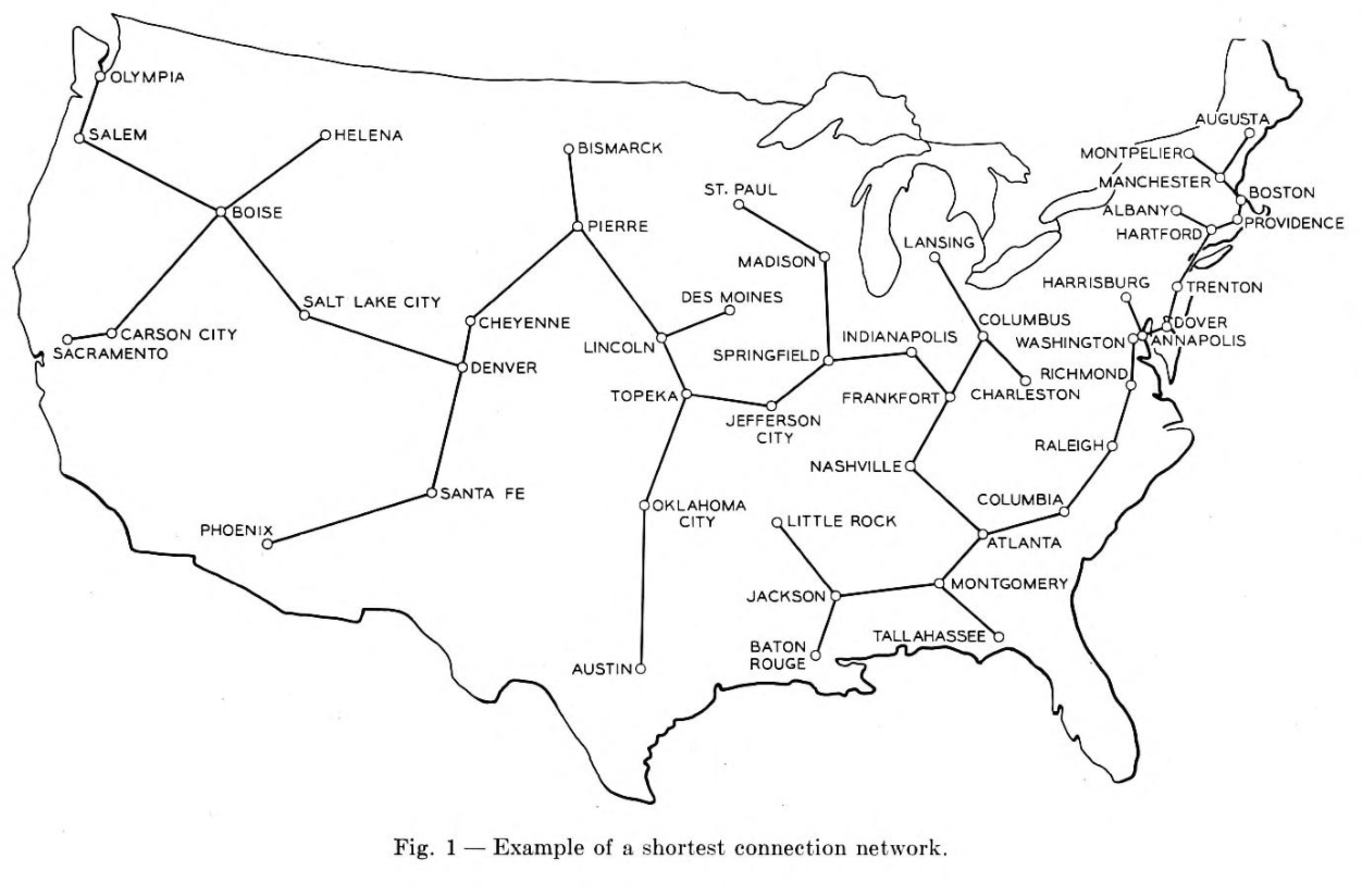
Prim cited “large-scale communication” as the motivation for this algorithm, specifically the “Bell System leased-line”^[R.C. Prim, May 8, 1957 Shortest Connection Networks And Some Generalizations https://archive.org/details/bstj36-6-1389]. Leased lines were used primarily in a commercial setting which connected business offices that were geographically distant (IE in different cities or even states). Companies would want all offices to be connected but wanted to avoid having to lay an excessive amount of wire. Below is a figure which Prim used to motivate the need for the algorithm. This image depicts the minimum spanning tree which connect each of the US continental state capitals along with Washington D.C.
Algorithm
The basis of the algorithm is to start with only the nodes of the graph, then we do the following
- Choose a random node
- Grow your tree by one edge, selecting the smallest edge to connect to a node that is not yet in the tree. Repeat until all the nodes have been visited
Starting Graph
Resulting MST

Info
Uniqueness
You may have noticed that the minimum spanning tree that resulted from Kruskal’s algorithm differed from Prim’s algorithm. We have displaying them both below for reference.
| Kruskal | Prim |
|---|---|
|
|
|
While these are different, they are both valid. The trees both have cost 16. The MST of a graph will be unique, meaning there is only one, if none of the edges of the graph have the same weight.
Pseudocode
function PRIM(GRAPH, START)
    MST = GRAPH without the edges attribute(s)
    VISITED = empty set
    add START to VISITED
    AVAILEDGES = list of edges where START is the source
    sort AVAILEDGES
    while VISITED is not all of the nodes
        SMLEDGE = smallest edge in AVAILEDGES
        SRC = source of SMLEDGE
        TAR = target of SMLEDGE
        if TAR not in VISITED
            add SMLEDGE to MST as undirected edge
            add TAR to VISITED
            add the edges where TAR is the source to AVAILEDGES
        remove SMLEDGE from AVAILEDGES
        sort AVAILEDGES
    return MST
Traveling Salesperson
YouTube Video YouTube VideoWhile we won’t outline algorithms suited for solving the traveling salesperson problem (TSP), we will outline the premise of the problem. This problem was first posed in 1832, almost a two centuries ago, and is still quite prevalent. It is applicable to traveling routes, distribution networks, computer architecture and much more. The TSP is a seminal problem that has motivated many research breakthroughs, including Kruskals algorithm!
The motivation of the TSP is this: given a set of locations, what is the shortest path such that we can visit each location and end back where started?
Suppose we wanted to take a roadtrip with friends to every state capital in the continental US as well as Washington D.C. To save money and time, we would want to minimize the distance that we travel. Since we are taking a roadtrip, we would want to avoid frivolous driving. For example, if we start in Sacremento, CA we would not want to end the trip in Boston, MA. The trip should start and end at the same location for efficiency.
The figure below shows the shortest trip that visits each state capital and Washington D.C. once. In this example, we can start where ever we like and will end up where we started.
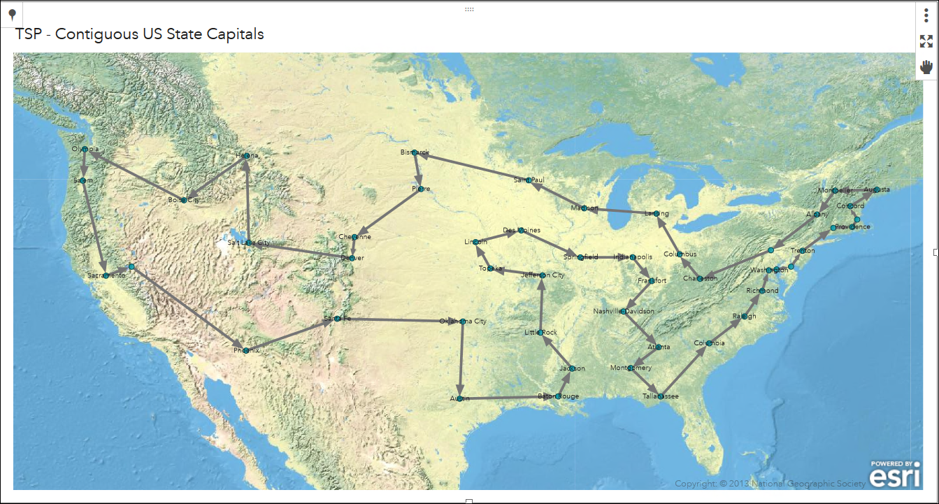 ^[PatriciaNeri, August 2018 https://communities.sas.com/t5/SAS-Communities-Library/What-is-the-shortest-tour-that-visits-only-once-the-48/ta-p/490231]
In this problem, it is easy to get overwhelmed by all of the possibilities. Since there are 49 cities to visit, there are over 6.2*10^60 possibilities. For reference, 10^12 is equivalent to one trillion! Thus, we need an algorithmic approach to solve this problem as opposed to a brute force method.