Homepage
CC 315 Textbook
This is the textbook for CC 315.
This is the textbook for CC 315.
This page is the main page for the introductory material.
Instructor: Safia Malallah (safia AT ksu DOT edu) _I use she/her pronouns. If you need assistance, please send an email to safia @ ksu.edu, cc’ing cis115-help@KSUemailProd.onmicrosoft.com. Avoid using the Canvas email function, as emailing this way ensures that your message reaches all instructors for this course, guaranteeing a swifter response. You can expect a response by the end of the next business day; feel free to reach out again if you don’t receive a response within 24 business hours.
Office: DUE 2161
Virtual Office Hours: Schedule a meeting with me: https://calendly.com/safiamalallah Appointments held via Zoom.
Advanced data structures and related algorithms. Formal software development methods and software engineering fundamentals. Introduction to requirements analysis processes that provide the specification of algorithmic requirements.
This course introduces advanced data structures, such as trees, graphs, and heaps. Several new algorithms using these data structures are covered. Students also learn software development methods and software engineering fundamentals and use those skills to develop projects of increasing size and scope effectively.
These courses are being taught 100% online, and each module is self-paced. There may be some bumps in the road as we refine the overall course structure. Students will work at their own pace through a set of modules, with approximately one module being due each week. Material will be provided in the form of recorded videos, online tutorials, links to online resources, and discussion prompts. Each module will include a coding project or assignment, many of which will be graded automatically through Codio. Assignments may also include portions which will be graded manually via Canvas or other tools.
The assigments for this course is delivered through Python programming language.
All activities are individual effort. ‘Group’ work is not permitted.
Students are granted the opportunity to
You are expected to use the Codio Editor. It is deliberately feature poor to place the burden of programming syntax, vocabulary and logic flow on the student. DO NOT CUT AND PASTE into the editor while coding your projects.
Exception, you may cut and paste from Codio, so if you accidently delete the starter code, or want to modify a section of code you made in the tutorial. INCLUDE a comment stating from where you ‘sourced’ the pasted section.
from Codio tutorial 3.4.P.7 with open(sys.argv[1]) as input_file:
try:

    reader = input_file.readlines()

except:

    reader = sys.stdin
In theory, each student begins the course with an A. As you submit work, you can either maintain your A (for good work) or chip away at it (for less adequate or incomplete work). In practice, each student starts with 0 points in the gradebook and works upward toward a final point total earned out of the possible number of points. In this course, each assignment constitutes a portion of the final grade, as detailed below:
Up to 5% of the total grade in the class is available as extra credit. See the Extra Credit - Bug Bounty assignment for details.
Letter grades will be assigned following the standard scale:
The Projects you submit in Codio may have both an automatic and manual grading component.
Automatic Components: Codio automatically checks certain aspects of your code’s structure and functionality. The grade assigned by Codio is generally the ceiling of the score you can receive.
Manual Components: Once submitted your code may be reviewed and deductions take for:
Forbidden statements/Required statements: Some assignments may prohibit the use of certain built in functions and methods. Others may require the use of certain libraries and methods. Using prohibited statements and or skipping required statements will result in a ZERO for the project.
Cutting and Pasting into the Codio IDE (Project assignments): You are expected to do your work in Codio. Cutting and pasting from outside Codio is prohibited, may result in a zero and will trigger a closer plagiarism review.
Running from the terminal: Codio does not typically check for proper terminal input behavior. A project that does not compile and/or run from the terminal will result in a 25% reduction in your final score. The project should work for the sample inputs, and should not crash or print extraneous information.
Having extra methods/missing required methods: up to 10% deduction
Style Guide: see Pages
Read this late work policy very carefully! If you are unsure how to interpret it, please contact the instructors via the help email. Not understanding the policy does not mean that it won’t apply to you!
Since this course is entirely online, students may work at any time and at their own pace through the modules. However, to keep everyone on track, there will be approximately one module due each week. Each graded item in the module will have a specific due date specified. All of the components of a module will be subject to the late policy if the module is submitted late. This penalty will be assessed via a single separate assignment entry in the gradebook, containing the sum of all grade reductions in the course for that student. Late assignments will not be accepted if they have been submitted more than 3 days after the due date, unless a special reason is provided and prior approval for an extension has been obtained before the due date.
For the purposes of recordkeeping, the submission time of the confirmation quiz in each module will be used to establish the completion time of the entire module in case of a discrepancy. This is because Codio may update submission times when assignments are regraded, but the quiz in Canvas should only be completed once.
However, even if a module is not submitted on time, it must still be completed before a student is allowed to begin the next module. So, students should take care not to get too far behind, as it may be very difficult to catch up.
Finally, all course work must be submitted on or before the last day of the semester in which the student is enrolled in the course in order for it to be graded on time.
If you have extenuating circumstances, please discuss them with the instructor as soon as they arise so other arrangements can be made. If you find that you are getting behind in the class, you are encouraged to speak to the instructor for options to make up missed work.
Students should strive to complete this course in its entirety before the end of the semester in which they are enrolled. However, since retaking the course would be costly and repetitive for students, we would like to give students a chance to succeed with a little help rather than immediately fail students who are struggling.
If you are unable to complete the course in a timely manner, please contact the instructor to discuss an incomplete grade. Incomplete grades are given solely at the instructor’s discretion. See the official K-State Grading Policy for more information. In general, poor time management alone is not a sufficient reason for an incomplete grade.
Unless otherwise noted in writing on a signed Incomplete Agreement Form, the following stipulations apply to any incomplete grades given in Computational Core courses:
All graded work is individual effort. You are authorized to use:
course’s materials, direct web-links from this course the appropriate languages documentation (https://docs.python.org/3/ or https://docs.oracle.com/javase/Links to an external site.) Email help received through 315 help email, CC - Instructors, GTAs Zoom/In-person help received from Instructors or GTA ACM help session (an on campus only resource) Most Tuesdays in EH 1116, 6:30PM. Tutors from the Academic Assistance Center or provided by K-State Athletics Use of on-line solutions whether for reference or code is prohibited. Use of previous semester’s answers, whether your own or another student’s is prohibited. Use of code-completion/suggestion tool’s, other than those we have installed in the Codio editor, is prohibitied.
CC-315 is a three-hour course; most students find it more time consuming than CC-310.
Modules have been assigned so that the average amount of work (hours), based on past student performance, is somewhat consistent.
You may work ahead, but modules must be worked strictly in order. Also, if you are far ahead, it may take a bit longer to get help. We review the lessons every week so the support you get is not ’too advanced’; if you are pretty far ahead, we will need to ‘catch up’ to where you are to provide support.
Please note, modules are not equally weighted, some are worth far more than others.
To participate in this course, students must have access to a modern web browser and broadband internet connection. All course materials will be provided via Canvas and Codio. Modules may also contain links to external resources for additional information, such as programming language documentation.
The details in this syllabus are not set in stone. Due to the flexible nature of this class, adjustments may need to be made as the semester progresses, though they will be kept to a minimum. If any changes occur, the changes will be posted on the Canvas page for this course and emailed to all students.
The statements below are standard syllabus statements from K-State and our program. The latest versions are available online here.
Kansas State University has an Honor and Integrity System based on personal integrity, which is presumed to be sufficient assurance that, in academic matters, one’s work is performed honestly and without unauthorized assistance. Undergraduate and graduate students, by registration, acknowledge the jurisdiction of the Honor and Integrity System. The policies and procedures of the Honor and Integrity System apply to all full and part-time students enrolled in undergraduate and graduate courses on-campus, off-campus, and via distance learning. A component vital to the Honor and Integrity System is the inclusion of the Honor Pledge which applies to all assignments, examinations, or other course work undertaken by students. The Honor Pledge is implied, whether or not it is stated: “On my honor, as a student, I have neither given nor received unauthorized aid on this academic work.” A grade of XF can result from a breach of academic honesty. The F indicates failure in the course; the X indicates the reason is an Honor Pledge violation.
For this course, a violation of the Honor Pledge will result in sanctions such as a 0 on the assignment or an XF in the course, depending on severity. Actively seeking unauthorized aid, such as posting lab assignments on sites such as Chegg or StackOverflow, or asking another person to complete your work, even if unsuccessful, will result in an immediate XF in the course.
This course assumes that all your course work will be done by you. Use of AI text and code generators such as ChatGPT and GitHub Copilot in any submission for this course is strictly forbidden unless explicitly allowed by your instructor. Any unauthorized use of these tools without proper attribution is a violation of the K-State Honor Pledge.
We reserve the right to use various platforms that can perform automatic plagiarism detection by tracking changes made to files and comparing submitted projects against other students’ submissions and known solutions. That information may be used to determine if plagiarism has taken place.
At K-State it is important that every student has access to course content and the means to demonstrate course mastery. Students with disabilities may benefit from services including accommodations provided by the Student Access Center. Disabilities can include physical, learning, executive functions, and mental health. You may register at the Student Access Center or to learn more contact:
Students already registered with the Student Access Center please request your Letters of Accommodation early in the semester to provide adequate time to arrange your approved academic accommodations. Once SAC approves your Letter of Accommodation it will be e-mailed to you, and your instructor(s) for this course. Please follow up with your instructor to discuss how best to implement the approved accommodations.
All student activities in the University, including this course, are governed by the Student Judicial Conduct Code as outlined in the Student Governing Association By Laws, Article V, Section 3, number 2. Students who engage in behavior that disrupts the learning environment may be asked to leave the class.
At K-State, faculty and staff are committed to creating and maintaining an inclusive and supportive learning environment for students from diverse backgrounds and perspectives. K-State courses, labs, and other virtual and physical learning spaces promote equitable opportunity to learn, participate, contribute, and succeed, regardless of age, race, color, ethnicity, nationality, genetic information, ancestry, disability, socioeconomic status, military or veteran status, immigration status, Indigenous identity, gender identity, gender expression, sexuality, religion, culture, as well as other social identities.
Faculty and staff are committed to promoting equity and believe the success of an inclusive learning environment relies on the participation, support, and understanding of all students. Students are encouraged to share their views and lived experiences as they relate to the course or their course experience, while recognizing they are doing so in a learning environment in which all are expected to engage with respect to honor the rights, safety, and dignity of others in keeping with the K-State Principles of Community.
If you feel uncomfortable because of comments or behavior encountered in this class, you may bring it to the attention of your instructor, advisors, and/or mentors. If you have questions about how to proceed with a confidential process to resolve concerns, please contact the Student Ombudsperson Office. Violations of the student code of conduct can be reported using the Code of Conduct Reporting Form. You can also report discrimination, harassment or sexual harassment, if needed.
This is our personal policy and not a required syllabus statement from K-State. It has been adapted from this statement from K-State Global Campus, and theRecurse Center Manual. We have adapted their ideas to fit this course.
Online communication is inherently different than in-person communication. When speaking in person, many times we can take advantage of the context and body language of the person speaking to better understand what the speaker means, not just what is said. This information is not present when communicating online, so we must be much more careful about what we say and how we say it in order to get our meaning across.
Here are a few general rules to help us all communicate online in this course, especially while using tools such as Canvas or Discord:
As a participant in course discussions, you should also strive to honor the diversity of your classmates by adhering to the K-State Principles of Community.
Kansas State University is committed to maintaining academic, housing, and work environments that are free of discrimination, harassment, and sexual harassment. Instructors support the University’s commitment by creating a safe learning environment during this course, free of conduct that would interfere with your academic opportunities. Instructors also have a duty to report any behavior they become aware of that potentially violates the University’s policy prohibiting discrimination, harassment, and sexual harassment, as outlined by PPM 3010.
If a student is subjected to discrimination, harassment, or sexual harassment, they are encouraged to make a non-confidential report to the University’s Office for Institutional Equity (OIE) using the online reporting form. Incident disclosure is not required to receive resources at K-State. Reports that include domestic and dating violence, sexual assault, or stalking, should be considered for reporting by the complainant to the Kansas State University Police Department or the Riley County Police Department. Reports made to law enforcement are separate from reports made to OIE. A complainant can choose to report to one or both entities. Confidential support and advocacy can be found with the K-State Center for Advocacy, Response, and Education (CARE). Confidential mental health services can be found with Lafene Counseling and Psychological Services (CAPS). Academic support can be found with the Office of Student Life (OSL). OSL is a non-confidential resource. OIE also provides a comprehensive list of resources on their website. If you have questions about non-confidential and confidential resources, please contact OIE at equity@ksu.edu or (785) 532–6220.
Kansas State University is a community of students, faculty, and staff who work together to discover new knowledge, create new ideas, and share the results of their scholarly inquiry with the wider public. Although new ideas or research results may be controversial or challenge established views, the health and growth of any society requires frank intellectual exchange. Academic freedom protects this type of free exchange and is thus essential to any university’s mission.
Moreover, academic freedom supports collaborative work in the pursuit of truth and the dissemination of knowledge in an environment of inquiry, respectful debate, and professionalism. Academic freedom is not limited to the classroom or to scientific and scholarly research, but extends to the life of the university as well as to larger social and political questions. It is the right and responsibility of the university community to engage with such issues.
Kansas State University is committed to providing a safe teaching and learning environment for student and faculty members. In order to enhance your safety in the unlikely case of a campus emergency make sure that you know where and how to quickly exit your classroom and how to follow any emergency directives. Current Campus Emergency Information is available at the University’s Advisory webpage.
K-State has many resources to help contribute to student success. These resources include accommodations for academics, paying for college, student life, health and safety, and others. Check out the Student Guide to Help and Resources: One Stop Shop for more information.
Student academic creations are subject to Kansas State University and Kansas Board of Regents Intellectual Property Policies. For courses in which students will be creating intellectual property, the K-State policy can be found at University Handbook, Appendix R: Intellectual Property Policy and Institutional Procedures (part I.E.). These policies address ownership and use of student academic creations.
Your mental health and good relationships are vital to your overall well-being. Symptoms of mental health issues may include excessive sadness or worry, thoughts of death or self-harm, inability to concentrate, lack of motivation, or substance abuse. Although problems can occur anytime for anyone, you should pay extra attention to your mental health if you are feeling academic or financial stress, discrimination, or have experienced a traumatic event, such as loss of a friend or family member, sexual assault or other physical or emotional abuse.
If you are struggling with these issues, do not wait to seek assistance.
For Kansas State Salina Campus:
For Global Campus/K-State Online:
K-State has a University Excused Absence policy (Section F62). Class absence(s) will be handled between the instructor and the student unless there are other university offices involved. For university excused absences, instructors shall provide the student the opportunity to make up missed assignments, activities, and/or attendance specific points that contribute to the course grade, unless they decide to excuse those missed assignments from the student’s course grade. Please see the policy for a complete list of university excused absences and how to obtain one. Students are encouraged to contact their instructor regarding their absences.
© The materials in this online course fall under the protection of all intellectual property, copyright and trademark laws of the U.S. The digital materials included here come with the legal permissions and releases of the copyright holders. These course materials should be used for educational purposes only; the contents should not be distributed electronically or otherwise beyond the confines of this online course. The URLs listed here do not suggest endorsement of either the site owners or the contents found at the sites. Likewise, mentioned brands (products and services) do not suggest endorsement. Students own copyright to what they create.
This page is the main page for the Strings and StringBuilders Section
This page is the main page for the Strings and StringBuilders chapter
In CC310 we covered various data structures: stacks, sets, lists, queues, and hash tables. When we looked at these structures, we considered how to access elements within the structures, how we would create our own implementation of the structure, and tasks that these structures would be fitting for as well as ill fitting. Throughout this course we will introduce and implement a variety of data structures as we did in CC310.
We begin this course with an often overlooked structure: strings. By the end of this chapter, we will understand how strings are data structures, how we access elements, what types of tasks are appropriate for strings, and how we can improve on strings in our code.
In many data science positions, programmers often work with text-based data. Some examples of text-based data include biology for DNA sequencing, social media for sentiment classification, online libraries for citation networks, and many other types of businesses for data analytics. Currently, strings are often used for word embeddings, which determine how similar or dissimilar words are to one another. An industry leading software for this application is Tensorflow for Python, which generated the image below.
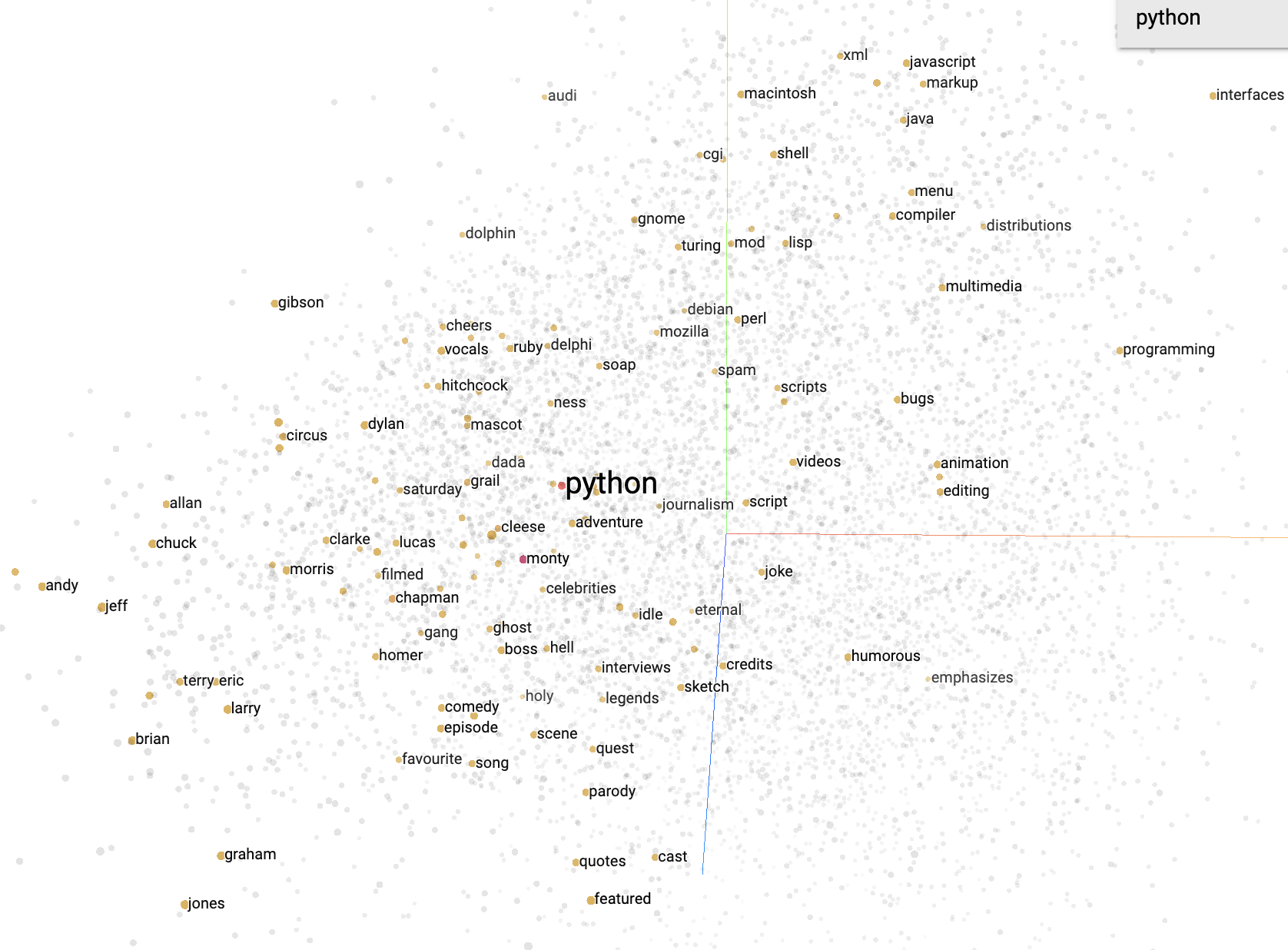
In an immense oversimplification, the process used for word embeddings is to read in a large amount of text and then use machine learning algorithms to determine similarity by using the words around each word. This impacts general users like us in search engines, streaming services, dating applications, and much more! For example, if you were to search Python topics in your search results may appear referring to the coding language, the reptile, the comedy troupe, and many more. When we use machine learning to determine word meanings, it is important that the data is first parsed correctly and stored in efficient ways so that we can access elements as needed. Understanding how to work with strings and problems that can arise with them is important to utilizing text successfully.
Reference: https://projector.tensorflow.org/
Strings are data structures which store an ordered set of characters. Recall that a character can be a: letter, number, symbol, punctuation mark, or white space. Strings can contain any number and any combination of these. As such, strings can be single characters, words, sentences, and even more.
Let’s refresh ourselves on how strings work, starting with the example string: s = "Go Cats!".
| Character | G | o | C | a | t | s | ! | |
| Index | 0 | 1 | 2 | 3 | 4 | 5 | 6 | 7 |
As with other data structures, we can access elements within the string itself. Using the example above, s[0] would contain the character ‘G’, s[1] would contain the character ‘o’, s[2] would contain the character ’ ‘, and so on.
We can determine the size of a string by using length functions; in our example, the length of s would be 8. It is also important to note that when dealing with strings, null is not equivalent to “”. For string s = "", the length of s would be 0. However for string s = null, accessing the length of s would return an error that null has no length property.
We can also add to strings or append on a surface level; though it is not that simple behind the scenes. The String class is immutable. This means that changes will not happen directly to the string; when appending or inserting, code will create a new string to hold that value. More concisely, the state of an immutable object cannot change.
We cannot assign elements of the string directly and more broadly for any immutable object. For example, if we wanted the string from our example to be ‘Go Cat!!’, we cannot assign the element through s[6] = '!'. This would result in an item assignment error.
For an example, consider string s = ‘abc’. If we then state in code s = s + ‘123’, this will create a new place in memory for the new definition of s. We can verify this in code by using the id() function.
string s = 'abc'
id(s)
Output: 140240213073680 #may be different on your personal device

string s = s + '123'
id(s)
Output: 140239945470168
While on the surface it appears that we are working with the same variable, our code will actually refer to a different one. There are many other immutable data types as well as mutable data types.
On the topic of immutable, we can also discuss the converse: mutable objects. Being a mutable object means that the state of the object can change. In CC310, we often worked with arrays to implement various data structures. Arrays are mutable, so as we add, change, or remove elements from an array, the array changes its state to accommodate the change rather than creating a new location in memory.
| Data Type | Immutable? |
|---|---|
| Lists | ☐ |
| Sets | ☐ |
| Byte Arrays | ☐ |
| Dictionaries | ☐ |
| Strings | ☑ |
| Ints | ☑ |
| Floats | ☑ |
| Booleans | ☑ |
Reference: http://people.cs.ksu.edu/~rhowell/DataStructures/strings/strings.html
Consider the following block of pseudocode:
1. function APPENDER(NUMBER, BASE)
2. RESULT = ""
3. loop I from 1 to NUMBER
4. RESULT = RESULT + BASE
5. if I MOD 2 = 0
6. RESULT = RESULT + " "
7. else
8. RESULT = RESULT + ", "
9. end loop
10. return RESULT
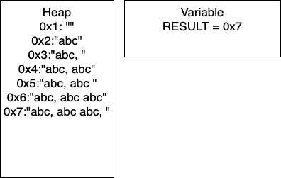
11. end functionLets step through the function call with APPENDER(4,'abc') and analyze the memory that the code takes.
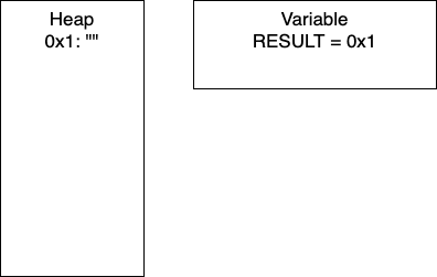
Recall that strings are reference variables. As such, string variables hold pointers to values and the value is stored in memory. For the following example, the HEAP refers to what is currently stored in memory and VARIABLE shows the current value of the variable RESULT.
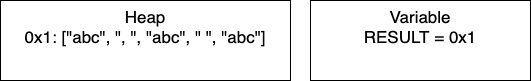
Initialization: In line two, we initialize RESULT as an empty string. In the heap, we have the empty string at memory location 0x1. Thus, RESULT is holding the pointer 0x1.
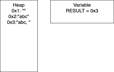
I = 1: Now we have entered the loop and on line 4, we add more characters to our string. At this point, we would have entry 0x2 in our heap and our variable RESULT would have the pointer 0x2. Continuing through the code, line 5 determines if I is divisible by 2. In this iteration I = 1, so we take the else branch. We again add characters to our string, resulting in a new entry in 0x3 and our variable RESULT containing the pointer 0x3. In total, we have written 8 characters. We then increment I and move to the next iteration.
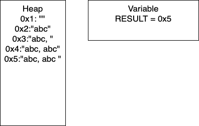
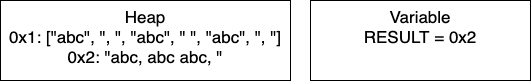
I = 2: We continue the loop and on line 4, we add more characters to our string. At this point, we would have entry 0x4 in our heap and our variable RESULT would have the pointer 0x4. Continuing through the code, line 5 determines if I is divisible by 2. In this iteration I = 2, so we take the if branch. We again add characters to our string, resulting in a new entry in 0x5 and our variable RESULT containing the pointer 0x5. In this iteration, we have written 17 characters. We then increment I and move to the next iteration of the loop.
I = 3: We continue the loop and on line 4, we add more characters to our string. At this point, we would have entry 0x6 in our heap and our variable RESULT would have the pointer 0x6. Continuing through the code, line 5 determines if I is divisible by 2. In this iteration I = 3, so we take the if branch. We again add characters to our string, resulting in a new entry in 0x7 and our variable RESULT containing the pointer 0x7. In this iteration, we have written 26 characters. We then increment I and thus I = 4 breaking out of the loop.
We can do some further analysis of the memory that is required for this particular block.
| Iteration | Memory Entries | Total Character Copies |
|---|---|---|
| 1 | 3 | 8 |
| 2 | 5 | 8 + 17 = 25 |
| 3 | 7 | 25 + 26 = 51 |
| 4 | 9 | 51 + 35 = 86 |
| . | . | . |
| n | 2n + 1 | (9n2 + 7n)/2 |
You need not worry about creating the equations! Based on this generalization, if the user wanted to do 100K iterations, say for gene sequencing, there would be (2x100,000 - 1) = 200,001 memory entries and (9x100,0002 + 7x100,000)/2 = 45 billion character copies. This behavior is not exclusive to strings; this will occur for any immutable type.
While this example is contrived, it is not too far off the mark. Another caveat to this analysis is that, depending on our programming language, there will be a periodic ‘memory collection’; there wont be 200K memory addresses occupied at one time. Writing to memory in this way can be costly in terms of time, which in industry is money.
As a result of being immutable, strings can be cumbersome to work with in certain applications. When long strings or strings that we are continually appending to, such as in the memory example, we end up creating a lot of sizable copies.
Recall from the memory example the block of pseudocode.
1. function APPENDER(NUMBER, BASE)
2.     RESULT = ""
3.     loop I from 1 to NUMBER
4.         RESULT = RESULT + BASE
5.         if I MOD 2 = 0
6.             RESULT = RESULT + " "
7.         else
8.             RESULT = RESULT + ", "
9.     end loop
10.    return RESULT
11. end function
In this example, what if we changed RESULT to a mutable type, say a list of strings for Python or a StringBuilder in Java. Once the loop is done, we can cast RESULT to a string. By changing just the one aspect of the code, we would make only one copy of RESULT and have far less character copies.
Java specifically has a StringBuilder class which was created for this precise reason.
Consider the following, and note the slight changes on lines 2, 4, 6, 8 and the additional line 10.
1. function APPENDER_LIST(NUMBER, BASE)
2. RESULT = []
3. loop I from 1 to NUMBER
4. RESULT.APPEND(BASE)
5. if I MOD 2 = 0
6. RESULT.APPEND(" ")
7. else
8. RESULT.APPEND(", ")
9. end loop
10. RESULT = "".JOIN(RESULT)
11. return RESULT
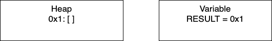
12. end functionNow consider APPENDER_LIST(4,‘abc’)
Initialization: We start by initializing the empty array. RESULT will hold the pointer 0x1.
I = 1: Now we have entered the loop and on line 4, we add more characters to our array. At this point, we would have only entry 0x1 in our heap and our variable RESULT would have the pointer 0x1. Continuing through the code, line 5 determines if I is divisible by 2. In this iteration I = 1, so we take the else branch. We again add characters to our array. In total, we have written 5 characters. We then increment I and move to the next iteration.
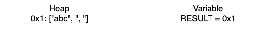
I = 2: We continue the loop and on line 4, we add more characters to our array. We still have just one entry in memory and our pointer is still 0x1. In this iteration, we have written 4 characters. We then increment I and move to the next iteration of the loop.
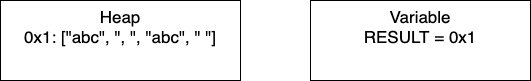
I = 3: We continue the loop and on line 4, we add more characters to our array. In this iteration, we have written 5 characters. We then increment I and thus I = 4 breaking out of the loop.
Post-Loop: Once the loop breaks, we join the array to create the final string. This creates a new place in memory and changes RESULT to contain the pointer 0x2.
We can do some further analysis of the memory that is required for this particular block.
| Iteration | Memory Entries | Character Copies |
|---|---|---|
| 1 | 2 | 8 |
| 2 | 2 | 17 |
| 3 | 2 | 26 |
| 4 | 2 | 35 |
| . | . | . |
| n | 2 | 9n - 1 |
Again, you need not worry about creating these equations for this course. To illustrate the improvement even more explicitly, let’s consider our previous example with 100K iterations. For APPENDER there were (2x100,000 - 1) = 200,001 memory entries and (9x100,0002 + 7x100,000)/2 = 45 billion character copies. For APPENDER_LIST we now have just 2 memory entries and (9x100,000 - 1) = 899,999 character copies. This dramatic improvement was a result of changing our data structure ever so slightly.
Reference: http://people.cs.ksu.edu/~rhowell/DataStructures/strings/stringbuilders.html
As a result of being immutable, strings can be cumbersome to work with in certain applications. When working with long strings or strings that we are continually appending to, such as in the memory example, we end up creating a lot of sizable copies.
Recall from the memory example the block of pseudocode.
1. function APPENDER(NUMBER, BASE)
2.     RESULT = ""
3.     loop I from 1 to NUMBER
4.         RESULT = RESULT + BASE
5.         if I MOD 2 = 0
6.             RESULT = RESULT + " "
7.         else
8.             RESULT = RESULT + ", "
9.     end loop
10.    return RESULT
11. end function
In this example, what if we changed RESULT to a mutable type, such as a StringBuilder in Java. Once the loop is done, we can cast RESULT to a string. By changing just the one aspect of the code, we would make only one copy of RESULT and have far less character copies.
Java specifically has a StringBuilder class which was created for this precise reason.
Consider the following, and note the slight changes on lines 2, 4, 6, 8 and the additional line 10.
1. function APPENDER_LIST(NUMBER, BASE)
2.     RESULT = []
3.     loop I from 1 to NUMBER
4.         RESULT.APPEND(BASE)
5.         if I MOD 2 = 0
6.             RESULT.APPEND(" ")
7.         else
8.             RESULT.APPEND(", ")
9.     end loop
10.    RESULT = "".JOIN(RESULT)
11.    return RESULT
12. end function
Now consider APPENDER_LIST(4,‘abc’)
Initialization: We start by initializing the empty array. RESULT will hold the pointer 0x1.
I = 1: Now we have entered the loop and on line 4, we add more characters to our array. At this point, we would have only entry 0x1 in our heap and our variable RESULT would have the pointer 0x1. Continuing through the code, line 5 determines if I is divisible by 2. In this iteration I = 1, so we take the else branch. We again add characters to our array. In total, we have written 5 characters. We then increment I and move to the next iteration.
I = 2: We continue the loop and on line 4, we add more characters to our array. We still have just one entry in memory and our pointer is still 0x1. In this iteration, we have written 4 characters. We then increment I and move to the next iteration of the loop.
I = 3: We continue the loop and on line 4, we add more characters to our array. In this iteration, we have written 5 characters. We then increment I and thus I = 4 breaking out of the loop.
Post-Loop: Once the loop breaks, we join the array to create the final string. This creates a new place in memory and changes RESULT to contain the pointer 0x2.
We can do some further analysis of the memory that is required for this particular block.
| Iteration | Memory Entries | Character Copies |
|---|---|---|
| 1 | 2 | 8 |
| 2 | 2 | 17 |
| 3 | 2 | 26 |
| 4 | 2 | 35 |
| . | . | . |
| n | 2 | 9n - 1 |
Again, you need not worry about creating these equations for this course. To illustrate the improvement even more explicitly, let’s consider our previous example with 100K iterations. For APPENDER there were (2x100,000 - 1) = 200,001 memory entries and (9x100,0002 + 7x100,000)/2 = 45 billion character copies. For APPENDER_LIST we now have just 2 memory entries and (9x100,000 - 1) = 899,999 character copies. This dramatic improvement was a result of changing our data structure ever so slightly.
Reference: http://people.cs.ksu.edu/~rhowell/DataStructures/strings/stringbuilders.html
To start this course, we have looked into strings. They are a very natural way to represent data, especially in real world applications. Often though, the datapoints can be very large and require multiple modifications. We also examined how strings work: element access, retrieving the size, and modifying them. We looked into some alternatives which included StringBuilders for Java and character arrays for Python.
To really understand this point, we have included a comparison. We have implemented the APPENDER and APPENDER_LIST functions in both Python and Java. For the Java implementation, we utilized StringBuilders.
1. function APPENDER(NUMBER, BASE)
2.     RESULT = ""
3.     loop I from 1 to NUMBER
4.         RESULT = RESULT + BASE
5.         if I MOD 2 = 0
6.             RESULT = RESULT + " "
7.         else
8.             RESULT = RESULT + ", "
9.     end loop
10.    return RESULT
11. end function
1. function APPENDER_LIST(NUMBER, BASE)
2. RESULT = []
3. loop I from 1 to NUMBER
4. RESULT.APPEND(BASE)
5. if I MOD 2 = 0
6. RESULT.APPEND(" ")
7. else
8. RESULT.APPEND(", ")
9. end loop
10. RESULT = "".JOIN(RESULT)
11. return RESULT
12. end functionFor the tests of 108 and 109 in Java, the string implementation took over 24 hours and the StringBuilder implementation ran out of memory. For these reasons, they are omitted from the figure.
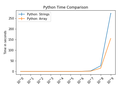
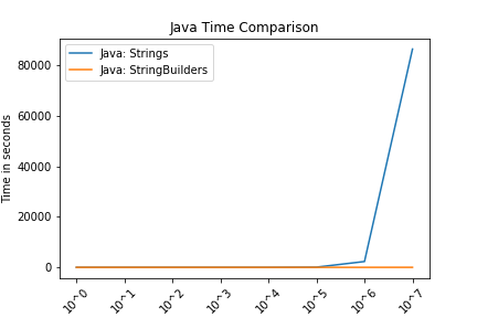
These figures compare Strings and lists for Python and Strings and StringBuilders for Java. The intention of these is not to compare Python and Java.
In both languages, we see that the string function and the respective alternative performed comparably until approximately 106 (1,000,000 characters). Again, these are somewhat contrived examples with the intention of understanding side effects of using strings.
As we have discussed, modern coding languages will have clean up protocols and memory management strategies. With the intention of this class in mind, we will not discuss the memory analysis in practice.
When modifying strings we need to be cognizant of how often we will be making changes and how large those changes will be. If we are just accessing particular elements or only doing a few modifications then using plain strings is a reasonable solution. However, if we are looking to build our own DNA sequence this is not a good way to go as strings are immutable.
This page is the main page for the Trees Section. This section has chapters which cover:
This page is the main page for Introduction to Trees
For the next data structure in the course, we will cover trees, which are used to show hierarchical data. Trees can have many shapes and sizes and there is a wide variety of data that can be organized using them. Real world data that is appropriate for trees can include: family trees, management structures, file systems, biological classifications, anatomical structures and much more.
We can look at an example of a tree and the relationships they can show. Consider this file tree; it has folders and files in folders.
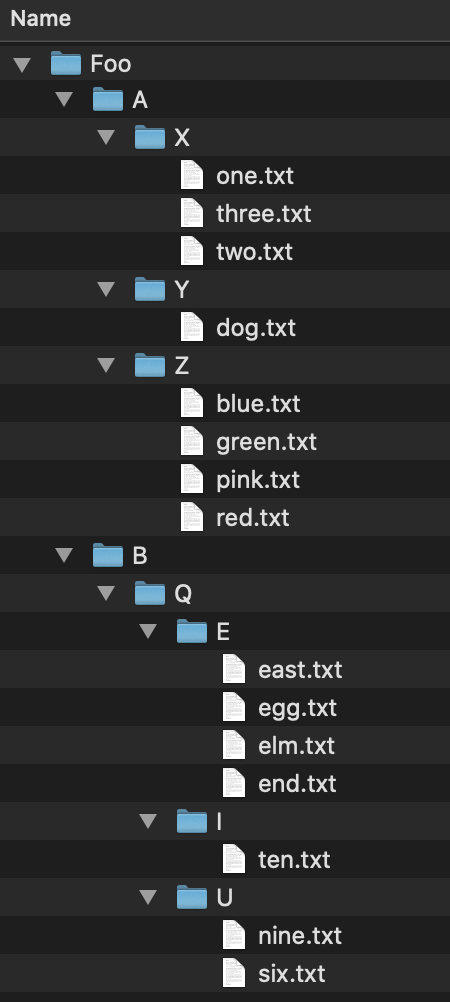
If we wanted to access the file elm.txt, we would have to follow this file path: Foo/B/Q/E/elm.txt. We can similarly store the file structure as a tree like we below. As before, if we wanted to get to the file elm.txt we would navigate the tree in the order: Foo -> B -> Q -> E -> elm.txt. As mentioned before, trees can be used on very diverse data sets; they are not limited to file trees!

In the last module we talked about strings which are a linear data structure. To be explicit, this means that the elements in a string form a line of characters. A tree, by contrast, is a hierarchal structure which is utilized best in multidimensional data. Going back to our file tree example, folders are not limited to just one file, there can be multiple files contained in a single folder- thus making it multidimensional.
Consider the string “abc123”; this is a linear piece of data where there is exactly one character after another. We can use trees to show linear data as well.

While trees can be used for linear data, it would be excessive and inefficient to implement them for single strings. In an upcoming module, we will see how we can use trees to represent any number of strings! For example, this tree below contains 7 words: ‘a’, ‘an’, ‘and’, ‘ant’, ‘any’, ‘all’, and ‘alp’.

In the next sections, we will discuss the properties of a tree data structure and how we would design one ourselves. Once we have a good understanding of trees and the properties of trees, we will implement our own.
To get ourselves comfortable in working with trees, we will outline some standard vocabulary. Throughout this section, we will use the following tree as a guiding example for visualizing the definitions.

Node - the general term for a structure which contains an item, such as a character or even another data structure.Edge - the connection between two nodes. In a tree, the edge will be pointing in a downward direction. This tree has five edges and six nodes. There is no limit to the number of nodes in a tree. The only stipulation is that the tree is
 fully connected. This means that there cannot be disjoint portions of the tree. We will look at examples in the next section.
A rule of thumb for discerning trees is this: if you imagine holding the tree up by the root and gravity took effect, then all edges must be pointing downward. If an edge is pointing upward, we will have a cycle within our structure so it will not be a tree.
Root - the topmost node of the tree To be a tree, there must be exactly one root. Having multiple roots, will result in a
 cycle or a tree that is not fully connected. In short, a cycle is a loop in the tree.
Parent - a node with an edge that connects to another node further from the root. We can also define the root of a tree with respect to this definition; Root: a node with no parent.Child - a node with an edge that connects to another node closer to the root.

 In a tree, child nodes must have exactly one parent node. If a child node has more than one parent, then a
 cycle will occur. If there is a node without a parent node, then this is necessarily the root node. There is no limit to the number of child nodes a parent node can have, but to be a parent node, the node must have at least one child node.Leaf - a node with no children.
 This tree has four leaves. There is no limit to how many leaves can be in a tree.
Degree
Degree of a node - the number of children a node has. The degree of a leaf is zero.Degree of a tree - the number of children the root of the tree has.
 The degree of the nodes are shown as the values on the nodes in this example. The degree of the tree is equal to the degree of the root. Thus, the degree for this tree is 2.
tree is defined recursively. This means that each child of the root is the root of another tree and the children of those are roots to trees as well. Again, this is a recursive definition so it will continue to the leaves. The leaves are also trees with just a single node as the root.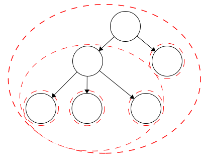 In our example tree, we have six trees. Each tree is outlined in a red dashed circle:
Trees can come in many shapes and sizes. There are, however some constraints to making a valid tree.
Any combination of the following represents a valid tree:
A tree with a single node; just a root,

A tree where each node has a single child, or

A tree where nodes have many children.

Below are some examples of invalid trees.
A cycle
 Again, cycles are essentially loops that occur in our tree. In this example, we see that our leaf has two parents. One way to determine whether your data structure has a cycle is if there is more than one way to get from the root to any node.
A cycle
 Here we can see another cycle. In this case, the node immediately after the root has two parents, which is a clue that a cycle exists. Another test
Two Roots
 Trees must have a single root. In this instance, it may look like we have a tree with two roots. Working through this, we also see that the node in the center has two parents.
Two Trees
 This example would be considered two trees, not a tree with two parts. In this figure, we have two fully connected components. Since they are not connected to each other, this is not a single tree.
Along with understanding how trees work, we want to also be able to implement a tree of our own. We will now outline key components of a tree class.
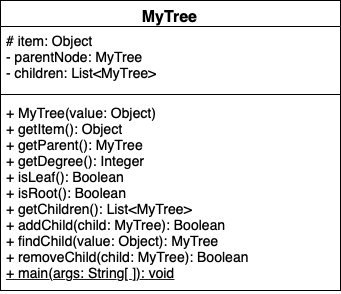
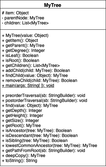
Recall that trees are defined recursively so we can build them from the leaves up where each leaf is a tree itself. Each tree will have three properties: the item it contains as an object, its parent node of type MyTree, and its children as a list of MyTrees. Upon instantiation of a new MyTree, we will set the item value and initialize the parent node to None and the children to an empty list of type MyTree.
Suppose that we wanted to construct the following tree.
 We would start by initializing each node as a tree with no parent, no children, and the item in this instance would be the characters. Then we build it up level by level by add the appropriate children to the respective parent.
Disclaimer: This implementation will not prevent all cycles. In the next module, we will introduce steps to prevent cycles and maintain true tree structures.
In this method, we will take a value as input and then check if that value is the item of a child of the current node. If the value is not the item for any of the node’s children then we should return none.
function FINDCHILD(VALUE)
    FOR CHILD in CHILDREN
        IF CHILD's ITEM is VALUE
            return  CHILD
    return NONE
end functionEach of these will be rather straight forward; children, item, and parent are all attributes of our node, so we can have a getter function that returns the respective values. The slightly more involved task will be getting the degree. Recall that the degree of a node is equal to the number of children. Thus, we can simply count the number of children and return this number for the degree.
We will have two functions to check the node type: one to determine if the node is a leaf and one to determine if it is a root. The definition of a leaf is a node that has no children. Thus, to check if a node is a leaf, we can simply check if the number of children is equal to zero. Similarly, since the definition of a root is a node with no parent, we can check that the parent attribute of the node is None.
When we wish to add a child, we must fisrt make sure we are able to add the child.
MyTreeWe will return true if the child was successfully added and false otherwise while raising the appropriate errors.
function ADDCHILD(CHILD)
    IF CHILD has PARENT
        throw exception
    IF CHILD is CHILD of PARENT
        return FALSE
    ELSE
        append CHILD to PARENT's children
        set CHILD's parent to PARENT
        return TRUE
end function
As an example, lets walk through the process of building the tree above:
a with item ‘A’b with item ‘B’c with item ‘C’d with item ‘D’e with item ‘E’f with item ‘F’g with item ‘G’h with item ‘H’i with item ‘I’g to tree dh to tree di to tree de to tree bf to tree bOnce we have completed that, visually, we would have the tree above and in code we would have:
a with parent_node = None, item = ‘A’, children = {b,c,d}b with parent_node = a, item = ‘B’, children = {e,f}c with parent_node = a, item = ‘C’, children = { }d with parent_node = a, item = ‘D’, children = {g,h,i}e with parent_node = b, item = ‘E’, children = { }f with parent_node = b, item = ‘F’, children = { }g with parent_node = d, item = ‘G’, children = { }h with parent_node = d, item = ‘H’, children = { }i with parent_node = d, item = ‘I’, children = { }Note: When adding a child we must currently be at the node we want to be the parent. Much like when you want to add a file to a folder, you must specify exactly where you want it. If you don’t, this could result in a wayward child.
In the case of removing a child, we first need to check that the child we are attempting to remove is an instance of MyTree. We will return true if we successfully remove the child and false otherwise.
function REMOVECHILD(CHILD)
    IF CHILD in PARENT'S children
        REMOVE CHILD from PARENT's children
        SET CHILD's PARENT to NONE
        return TRUE
    ELSE
        return FALSE
end function
As with adding a child, we need to ensure that we are in the ‘right place’ when attempting to remove a child. When removing a child, we are not ’erasing’ it, we are just cutting the tie from parent to child and child to parent. Consider removing d from a. Visually, we would have two disjoint trees, shown below:

In code, we would have:
a with parent_node = None, item = ‘A’, children = {b,c}b with parent_node = a, item = ‘B’, children = {e,f}c with parent_node = a, item = ‘C’, children = { }d with parent_node = None, item = ‘D’, children = {g,h,i}e with parent_node = b, item = ‘E’, children = { }f with parent_node = b, item = ‘F’, children = { }g with parent_node = d, item = ‘G’, children = { }h with parent_node = d, item = ‘H’, children = { }i with parent_node = d, item = ‘I’, children = { }In this module we have introduce vocabulary related to trees and what makes a tree a tree. To recap, we have introduced the following:
Child - a node with an edge that connects to another node closer to the root.Degree
Degree of a node - the number of children a node has. The degree of a leaf is zero.Degree of a tree - the number of children the root of the tree has.Edge - connection between two nodes. In a tree, the edge will be pointing in a downward direction.Leaf - a node with no children.Node - the general term for a structure which contains an item, such as a character or even another data structure.Parent - a node with an edge that connects to another node further from the root. We can also define the root of a tree with respect to this definition;Root - the topmost node of the tree; a node with no parent.Now we will work on creating our own implementation of a tree. These definitions will serve as a resource to us when we need refreshing on meanings; feel free to refer back to them as needed.
This page is the main page for Tree Traversal
In the last module, we covered the underlying vocabulary of trees and how we can implement our own tree. To recall, we covered: node, edge, root, leaf, parent, child, and degree.
For this module we will expand on trees and gain a better understanding of how powerful trees can be. As before, we will use the same tree throughout the module for a guiding visual example.

Many of the terms used in trees relate to terms used in family trees. Having this in mind can help us to better understand some of the terminology involved with abstract trees. Here we have a sample family tree.
Ancestor - The ancestors of a node are those reached from child to parent relationships. We can think of this as our parents and our parent’s parents, and so on.
Descendant - The descendants of a node are those reached from parent to child relationships. We can think of this as our children and our children’s children and so on.
Siblings - Nodes which share the same parent
A recursive program is broken into two parts:
In principle, the recursive case breaks the problem down into smaller portions until we reach the base case. Recursion presents itself in many ways when dealing with trees.
Trees are defined recursively with the base case being a single node. Then we recursively build the tree up. With this basis for our trees, we can define many properties using recursion rather effectively.
We can describe the sizes of trees and position of nodes using different terminology, like level, depth, and height.
Level - The level of a node characterizes the distance between the node and the root. The root of the tree is considered level 1. As you move away from the tree, the level increases by one.
Depth - The depth of a node is its distance to the root. Thus, the root has depth zero. Level and depth are related in that: level = 1 + depth.
Height of a Node - The height of a node is the longest path to a leaf descendant. The height of a leaf is zero.
Height of a Tree - The height of a tree is equal to the height of the root.
When working with multidimensional data structures, we also need to consider how they would be stored in a linear manner. Remember, pieces of data in computers are linear sequences of binary digits. As a result, we need a standard way of storing trees as a linear structure.

Path - a path is a sequence of nodes and edges, which connect a node with its descendant. We can look at some paths in the tree above:
Q to O: QROTraversal is a general term we use to describe going through a tree. The following traversals are defined recursively.
Pre refers to the root, meaning the root goes before the children.QWYUERIOPTA
Post refers to the root, meaning the root goes after the children.YUWEIOPRATQ

When we talk about traversals for general trees we have used the phrase ’the traversal could result in’. We would like to expand on why ‘could’ is used here. Each of these general trees are the same but their traversals could be different. The key concept in this is that for a general tree, the children are an unordered set of nodes; they do not have a defined or fixed order. The relationships that are fixed are the parent/child relationships.


| Tree | Preorder | Postorder |
|---|---|---|
| Tree 1 | QWYUERIOPTA |
YUWEIOPRATQ |
| Tree 2 | QETARIOPWUY |
EATIOPRUYWQ |
| Tree 3 | QROPITAEWUY |
OPIRATEUYWQ |
Again, we want to be able to implement a working version of a tree. From the last module, we had functions to add children, remove children, get attributes, and instantiate MyTree. We will now build upon that implementation to create a true tree.
A recursive program is broken into two parts:
Recall that in the previous module, we were not yet able to enforce the no cycle rule. We will now enforce this and add other tree functionality.
Disclaimer: In the previous module we had a disclaimer that stated our implementation would not prevent cycles. The following functions and properties will implement recursion. Thus, we can maintain legal tree structures!
In the first module, we discussed how we can define trees recursively, meaning a tree consists of trees. We looked at the following example. Each red dashed line represented a distinct tree, thus we had five trees within the largest tree making six trees in total.
We will use our existing implementation from the first module. Now to make our tree recursive, we will include more getter functions as well as functions for traversals and defining node relationships.
We can define each of these recursively.
YouTube VideoDepth - The depth of a node is its distance to the root. Thus, the root has depth zero.We can define the depth of a node recursively:
function GETDEPTH()
    if ROOT
        return 0
    else
        return 1 + PARENT.GETDEPTH()
end functionHeight of a Node - The height of a node is the longest path to a leaf descendant. The height of a leaf is zero.We can define the height of a node recursively:
function GETHEIGHT()
    if LEAF
        return 0
    else
        MAX = 0
        for CHILD in CHILDREN
            CURR_HEIGHT = CHILD.GETHEIGHT()
            if CURR_HEIGHT > MAX
                MAX = CURR_HEIGHT
        return 1 + MAX
end functionRoot - the topmost node of the tree; a node with no parent.We can define returning the root recursively:
function GETROOT()
    if ISROOT()
        return this tree
    else
        return PARENT.GETROOT()
end functionWe define the size of a tree as the total number of children.
function GETSIZE()
    SIZE = 1
    for CHILD in CHILDREN
        SIZE += CHILD.GETSIZE()
    return SIZE
end functionTo find a value within our tree, we will traverse down a branch as far as we can until we find the value. This will return the tree that has the value as the root.
function FIND(VALUE)
	if ITEM is VALUE
		return this node
	for CHILD in CHILDREN
		FOUND = CHILD.FIND(VALUE)
		if FOUND is not NONE
			return FOUND
	return NONE
end functionWe can determine many relationships within the tree. For example, given a node is it an ancestor of another node, a descendant, or a sibling?
YouTube VideoFor this function, we are asking: is this node an ancestor of the current instance? In this implementation, we will start at our instance and work down through the tree trying to find the node in question. With that in mind, we can define this process recursively:
function ISANCESTOR(TREE)
    if at TREE
        return true
    else if at LEAF
        return false
    else
        for CHILD in CHILDREN
            FOUND = CHILD.ISANCESTOR(TREE)
            if FOUND
                return true
        return false
end functionFor this function, we are asking: is this node a descendant of the current instance? In this implementation, we will start at our instance and work up through the tree trying to find the node in question. With that in mind, we can define this process recursively:
function ISDESCENDANT(TREE)
    if at TREE
        return true
    else if at ROOT
        return false
    else
        return PARENT.ISDESCENDANT(TREE)
end functionFor this function, we are asking: is this node a sibling of the current instance? To determine this, we can get the parent of the current instance and then get the parents children. Finally, we check if the node in question is in that set of children.
function ISSIBLING(TREE)
    if TREE in PARENT's CHILDREN
        return true
    else
        return false
end functionIn any tree, we can say that the root is a common ancestor to all of the nodes. We would like to get more information about the common ancestry of two nodes. For this function, we are asking: which node is the first place where this instance and the input node’s ancestries meet? Similar to our ISDESCENDANT, we will work our way up the tree to find the point where they meet
function LOWESTANCESTOR(TREE)
    if at TREE
        return TREE
    else if ISANCESTOR(TREE)
        return instance
    else if at ROOT
        return NONE
    else
        return PARENT.LOWESTANCESTOR(TREE)
end functionThis function will generate the path which goes from the root to the current instance.
function PATHFROMROOT(PATH)
    if NOT ROOT
        PARENT.PATHFROMROOT(PATH)
    append ITEM to PATH
end functionIn this module we have talked about two traversals: preorder and postorder. Both of these are defined recursively and the prefix refers to the order of the root.
In a preorder traversal, first we access the root and then run the preorder traversal on the children.
function PREORDER(RESULT)
    append ITEM to RESULT
    FOR CHILD in CHILDREN
           CHILD.PREORDER(RESULT)
end functionIn a postorder traversal, first we run the postorder traversal on the children then we access the root.
function POSTORDER(RESULT)
   FOR CHILD in CHILDREN
           CHILD.POSTORDER(RESULT)
   append ITEM to RESULT
end functionIn this section, we discussed more terminology related to trees as well as tree traversals. To recap the new vocabulary:
Ancestor - The ancestors of a node are those reached from child to parent relationships. We can think of this as our parents and the parents of our parents, and so on.Depth - The depth of a node is its distance to the root. Thus, the root has depth zero. Level and depth are related in that: level = 1 + depth.Descendant - The descendants of a node are those reached from parent to child relationships. We can think of this as our children and our children’s children and so on.Height of a Node - The height of a node is the longest path to a leaf descendant. The height of a leaf is zero.Height of a Tree - The height of a tree is equal to the height of the root.Level - The level of a node characterizes the distance the node is from the root. The root of the tree is considered level 1. As you move away from the tree, the level increases by one.Path - a sequence of nodes and edges which connect a node with its descendant.Siblings - Nodes which share the same parentTraversal is a general term we use to describe going through a tree. The following traversals are defined recursively.
This page is the main page for Tries
Recall that in the beginning of our discussions about trees, we looked at a small tree which contained seven strings as motivation for trees. This was a small example of a trie (pronounced ’try’) which is a type of tree that can represent sets of words.
Tries can be used for a variety of tasks ranging from leisurely games to accessibility applications. One example is ‘Boggle’ where players have a set of random letters and try to make as many words as possible. To code this game, we could create a vocabulary with a trie then traverse it to determine if players have played legal words. We can also use tries to provide better typing accessibility. Users could type a few letters of a word and our code could traverse the trie and suggest what letters or words they may be trying to enter.
A trie is a type of tree with some special characteristics. First it must follow the guidelines of being a tree:
The special characteristics for tries are:
In this course, we will display nodes with two circles as a convention to show which nodes are the end of words. Looking at this small trie as an example, we can determine which words are contained in our trie.
We start at the root, which will typically be an empty string, and traverse to a double lined node. "" -> a -> l -> l. Thus, the word ‘all’ is contained in our trie. Words within our tries do not have to end at leaves. For example, we can traverse "" -> a for the word ‘a’. We say this trie ‘contains’ seven words: ‘a’, ‘an’, ‘and’, ‘ant’, ‘any’, ‘all’, and ‘alp’.
Let’s look at another example of a trie. Here we have a larger trie. Think about how many words are captured by the tree; click the tree to see how many!
While the ‘a’, ‘at’, and ‘bee’ are words in the English language, they are not recognized by our trie. Depending on what the user intended, this could be by design. When we build our tries, users will input words that are valid for their vocabulary. Tries are not limited to the English language and can be created for any vocabulary.
To implement our own trie, we will build off of MyTree that we built recursively. We will add an attribute to our tree to reinforce which nodes are words and which ones are not.
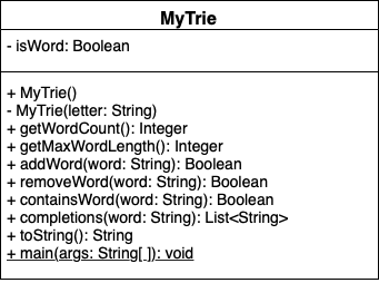
We have the existing attributes of MyTree: parent, children, and item. For MyTrie, we introduce the boolean attribute is_word to delineate if our trie is a word.
To add a word to our trie, we traverse through the trie letter by letter. We can define this recursively.
function ADDWORD(WORD)
    if WORD length is 0
        if already a word
            return false
        else
            set is_word to true
            return true
    else
        FIRST = first character of WORD
        REMAIN = remainder of WORD
        CHILD = FINDCHILD(FIRST)
        if CHILD is NONE
            NODE = new MyTrie with item equal FIRST
            insert NODE into our existing trie
            CHILD = NODE
        return CHILD.ADDWORD(REMAIN)
end functionSimilar to adding a word, we traverse our trie letter by letter. Once we get to the end of the word set is_word to false. If the word ends at a leaf, we will remove the leaf (then if the second to last character is a leaf, we remove the leaf and so on). If the word does not end in a leaf, meaning another word uses that node, we will not remove the node.
is_word is false and it is a leaf, remove the node.function REMOVEWORD(WORD)
if WORD length is 0
if already not a word
return false
else
set is_word to false
return true
else
FIRST = first character of WORD
REMAIN = remainder of WORD
CHILD = FINDCHILD(FIRST)
if CHILD is NONE
return false
else
RET = CHILD.REMOVEWORD(REMAIN)
if CHILD is not a word AND CHILD is a leaf
REMOVECHILD(CHILD)
return RET
end functionAgain, we will traverse the trie letter by letter. Once we get to the last letter, we can return that nodes is_word attribute. There is a chance that somewhere in our word, the letter is not a child of the previous node. If that is the case, then we return false.
function CONTAINSWORD(WORD)
    if WORD length is 0
        return `is_word`
    else
        FIRST = first character of WORD
        REMAIN = remainder of WORD
        CHILD = FINDCHILD(FIRST)
        if CHILD is NONE
            return false
        else
            return CHILD.CONTAINSWORD(REMAIN)
end functionFor this function, we want to get the total number of words that are contained within our trie. We will fan out through all of the children and count all of the nodes that have their is_word attribute equal to true.
function WORDCOUNT()
    COUNT = 0
    if is_word
        COUNT = 1
    for CHILD in CHILDREN
        COUNT += CHILD.WORDCOUNT()
    return COUNT
end functionNext, we want to get the longest word contained in our trie. To do this, we will recurse each child and find the maximum length of the child.
function MAXWORD()
    if LEAF and is_word
        return 0
    else
        MAX = -1
        for CHILD in CHILDREN
            COUNT = CHILD.MAXWORD()
            if COUNT greater than MAX
                MAX = COUNT
        return MAX + 1
end functionThis function will act as an auto-complete utility of sorts. A user will input a string of characters and we will return all of the possible words that are contained in our trie. This will happen in two phases. First, we traverse the trie to get to the end of the input string (lines 1-12). The second portion then gets all of the words that are contained after that point in our trie (lines 14-21).
function COMPLETIONS(WORD)
1.    if WORD length greater than 0
2.        FIRST = first character of WORD
3.        REMAIN = remainder of WORD
4.        CHILD = FINDCHILD(FIRST)
5.        if CHILD is none
6.            return []
7.        else
8.            COMPLETES = CHILD.COMPLETIONS(REMAIN)
9.            OUTPUT = []
10.            for COM in COMPLETES
11.                append CHILD.item + COM to OUTPUT
12.            return OUTPUT
13.    else
14.        OUTPUT = []
15.        if is_word
16.            append ITEM to OUTPUT
17.        for CHILD in CHILDREN
18.            COMPLETES = CHILD.COMPLETIONS("")
19.            for COM in COMPLETES
20.                append CHILD.item + COM to OUTPUT
21.        reutrn OUTPUT
end functionThis page is the main page for Binary Trees

A binary tree is a type of tree with some special conditions. First, it must follow the guidelines of being a tree:
The special conditions that we impose on binary trees are the following:
To reinforce these concepts, we will look at examples of binary trees and examples that are not binary trees.
 This is a valid binary tree. We have a single node, the root, with no children. As with general trees, binary trees are built recursively. Thus, each node and its child(ren) are trees themselves.
 This is also a valid binary tree. All of the left children are less than their parent. The node with item ‘10’ is also in the correct position as it is less than 12, 13, and 14 but greater than 9.
 We have the same nodes but our root is now 12 whereas before it was 14. This is also a valid binary tree.
 Here we have an example of a binary tree with alphabetical items. As long as we have items which have a predefined order, we can organize them using a binary tree.
 We may be inclined to say that this is a binary tree: each node has 0, 1, or 2 children and amongst children and parent nodes, the left child is smaller than the parent and the right child is greater than the parent. However, in binary trees, all of the nodes in the left tree must be smaller than the root and all of the nodes in the right tree must be larger than the root. In this tree,
 D is out of place. Node D is less than node T but it is also less than node Q. Thus, node D must be on the right of node Q.
 In this case, we do not have a binary tree. This does fit all of the criteria for being a tree but not the criteria for a binary tree. Nodes in binary trees can have at most 2 children. Node
 30 has three children.
In the first module we discussed two types of traversals: preorder and postorder. Within that discussion, we noted that for general trees, the preorder and postorder traversal may not be unique. This was due to the fact that children nodes are an unordered set.
We are now working with binary trees which have a defined child order. As a result, the preorder and postorder traversals will be unique! These means that for a binary tree when we do a preorder traversal there is exactly one string that is possible. The same applies for postorder traversals as well.
Recall that these were defined as such:
Now for binary trees, we can modify their definitions to be more explicit:
Let’s practice traversals on the following binary tree.


Since we have fixed order on the children, we can introduce another type of traversal: in-order traversal.
In-order Traversal:

Our implementation of binary trees will inherit from our MyTree implementation as binary trees are types of trees. Thus, MyBinaryTree will have the functionality of MyTree in addition to the following.
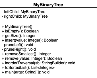
The binary tree has two attributes
MyBinaryTree, the item should be less than the item of the parent.MyBinaryTree, the item should be greater than the item of the parent.Get Size
MyTree size function. If the tree is empty then we return zero. If the tree is not empty then call the MyTree size function.Is Empty
To Sorted List
function TOSORTEDLIST()
    LIST = []
    if there`s LEFTCHILD
        LIST = LIST + LEFTCHILD.TOSORTEDLIST
    LIST = LIST + ITEM
    if there`s RIGHTCHILD
        LIST = LIST + RIGHTCHILD.TOSORTEDLIST
return LISTWhen inserting children to a binary tree, we must take some special considerations. All of the node items in the left tree must be less than the parent node item and all of the node items in the right tree must be greater than the parent node item.
The general procedure for adding a child is the following:
Suppose that we have the following tree and we want to add a node with item ‘85’. Click the binary tree to see the resulting tree.
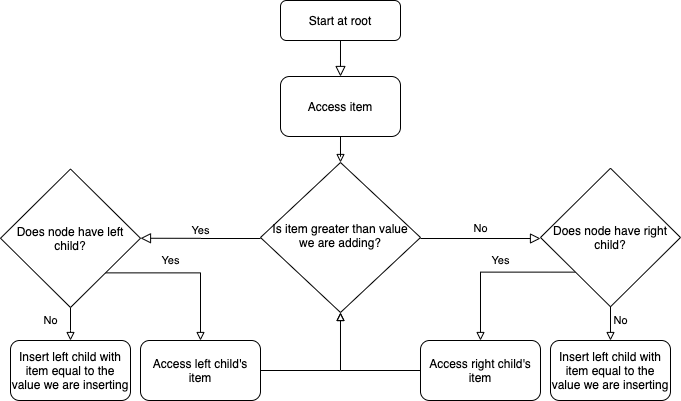
function INSERT(VALUE)
    if node is empty:
        set nodes item to value
    else:
        if node.ITEM is VALUE
            return false
        else if node.ITEM > VALUE
            LC = node`s left child
            if LC is NONE
                CHILD = new BINARYTREE with root.ITEM equal VALUE
                add CHILD to nodes children
                set node.LEFTCHILD equal to CHILD
                return true
            else
                return LC.INSERT(VALUE)
        else
            RC = node`s right child
            if RC is NONE
                CHILD = new BINARYTREE with root.ITEM equal VALUE
                add CHILD to nodes children
                set node.RIGHTCHILD equal to CHILD
                return true
            else
                return RC.INSERT(VALUE)
end function
Removing children is not as straightforward as inserting them. The general procedure for removing a child is to replace that nodes value with its smallest right descendant. First we will traverse the binary tree until we find the node with the value we are trying to remove (lines 18-32 below). Then we have three separate cases, discussed in detail below.
Removing a leaf is the most straightforward. We remove the value from the node and then sever the connection between parent and child. (lines 5-7 below)
Suppose we have this binary tree and we want to remove value 5. What do you think the resulting binary tree will look like? Click the binary tree to see the result.
When we remove a value from a node that does not have a right child, we cannot replace the value with the smallest right child. In this instance we will instead replace the value with the smallest left child then prune the tree to clean it up. Once we replace the value, we must switch the node’s left child to be the right child in order to maintain proper binary tree structure. (lines 8-13 below)
Suppose we have this binary tree and we want to remove value 4. What do you think the resulting binary tree will look like? Click the binary tree to see the result.
When we remove a value from a node that has a right child, we can replace the value with the nodes smallest right child. (Lines 14-17 Below)
Suppose we have this binary tree and we want to remove value 10. What do you think the resulting binary tree will look like? Click the binary tree to see the result.
1. function REMOVE(VALUE)
2.    if node is empty:
3.        error
4.    if node.ITEM is VALUE
5.        if node is a leaf
6.            set node.ITEM to none
7.            return TRUE
8.        else if node has no right child
9.            node.ITEM = LEFTCHILD.REMOVESMALLEST()
10.           prune left-side
11.           store left child in right child
12.           set left child to none
13.           return TRUE
14.        else
15.            node.ITEM = RIGHTCHILD.REMOVESMALLEST()
16.            prune right-side
17.            return TRUE
18.    else
19.        if node.ITEM > VALUE
20.            if node has LEFTCHILD
21.                SUCCESS = LEFTCHILD.REMOVE(VALUE)
22.                prune left-side
23.                return SUCCESS
24.            else
25.                return FALSE
26.        else
27.            if node has RIGHTCHILD
28.                SUCCESS = RIGHTCHILD.REMOVE(VALUE)
29.                prune right-side
30.                return SUCCESS
31.            else
32.                return FALSE
33. end functionWe use the pruning functions to severe the tie between parent and child nodes.
function PRUNERIGHT()
    if RIGHTCHILD has no value
        REMOVECHILD(RIGHTCHILD)
        set this nodes RIGHTCHILD former RIGHTCHILDs RIGHTCHILD
        if RIGHTCHLID is not none
            ADDCHILD(RIGHTCHILD)
end function
function PRUNELEFT()
if LEFTCHILD has no value
REMOVECHILD(LEFTCHILD)
set this nodes LEFTCHILD former LEFTCHILDs RIGHTCHILD
if LEFTCHILD is not none
ADDCHILD(LEFTCHILD)
end functionWe use the remove smallest function to retrieve the smallest value in the binary tree which will replace our value.
function REMOVESMALLEST()
    if node has left child
        REPLACEMENT = LEFTCHILD.REMOVESMALLEST
        prune left-side
        return REPLACEMENT
    else
        REPLACEMENT = node.ITEM
        if node has right child
            node.ITEM = RIGHTCHILD.REMOVESMALLEST()
            prune right-side
        else
            node.ITEM = NONE
        return REPLACEMENT
end function
While this is a valid binary tree, it is not balanced. Let’s look at the following tree.
We have the same nodes but our root is now 12 whereas before it was 14. This is a valid binary tree. We call this a balanced binary tree. A balanced binary tree looks visually even amongst the left and right trees in terms of number of nodes.
Note: Balancing is not necessary for a valid binary tree. It is, however, important in terms of time efficiency to have a balanced tree. For example, the number of actions when inserting an element is about the same as the number of levels in the tree. If we tried to add the value 11 into the unbalanced tree, we would traverse 5 nodes. If we tried to add the value 11 in to the balanced tree, we would traverse just 3 nodes.
We believe that balancing binary trees is out of the scope of this course. If you are interested in how we might balance a tree, feel free to check out these videos by Dr. Joshua Weese.
YouTube Video YouTube VideoThis page is the main page for Graphs: Matrix Representation
The next data structure we will introduce is a graph.

Graphs are multidimensional data structures that can represent many different types of data. We can use graphs to represent electronic circuits and wiring, transportation routes, and networks such as the Internet or social groups.
A popular and fun use of graphs is to build connections between people such as Facebook friends or even connections between performers. One example is the parlor game Six Degrees of Kevin Bacon. Players attempt to connect Kevin Bacon to other performers through movie roles in six people or less.

For example, Laurence Fishburne and Kevin Bacon are directly connected via ‘Mystic River’. Keanu Reeves and Kevin Bacon have never performed in the same film, but Keanu Reeves and Laurence Fishburne are connected via ‘The Matrix’. Thus, Keanu and Kevin are connected via Laurence.
In this module we will discuss graphs in more detail and build our own implementation of graphs.
We will discuss some of the basic terminology associated with graphs. Some of this vocabulary should feel familiar from the trees section; trees are a specific type of graph!
Nodes: Node is the general term for a structure which contains an item.
Size: The size of a graph is the number of nodes.Capacity: The capacity of a graph is the maximum number of nodes.Nodes can be, but are not limited to the following examples: - physical locations (IE Manhattan, Topeka, Salina), - computer components (IE CPU, GPU, RAM), or - people (IE Kevin Bacon, Laurence Fishburne, Emma Stone)
Edges: Edges are the connection between two nodes. Depending on the data, edges can represent physical distance, films, cost, and much more.
Adjacent: Node A and node B are said to be adjacent if there is an edge from node A to node B.Neighbors: The neighbors of a node are nodes which are adjacent to the node.Edges can be, but are not limited to: - physical distances, like the distance between cities or wiring between computer components, - cost, like bus fares, and - films, like the Six Degrees of Kevin Bacon example
Cycles: A cycle is a path where the first and last node are the only repeated nodes. More explicitly, this means that we start at node A and are able to end up back at node A.For example, we can translate the Amtrak Train Station Connections into a graph where the edges represent direct train station connections.
 ^[Generated using the Amtrak system map from 2018. This graph does not include all stations or connections.]
Within this context, we could say that Little Rock and Fort Worth are adjacent. The neighbors of San Antonio are Fort Worth, Los Angeles, and New Orleans. The Amtrak Train Graph has multiple cycles. One of these is Kansas City -> St. Louis -> Chicago -> Kansas City.
While trees are a type of graph, graphs can have more functionality than trees. For example, recall that to be a single tree, there could be no disconnected pieces.
Connectedness: Graphs do not require being fully connected. There can be disconnected portions within a graph. For example, the following graph shows all of the students in a sophomore biology class. There is an edge between two student nodes if they are Facebook friends.
Graphs can also have loops. In a tree, this would be like a node being its own parent, which is not an allowable condition.
Loops: Loops are edges which connect a node to itself. These can be useful in depicting graphs that show control flow in programming. In this example, node A is connected to node B and node A is connected to itself.
A weighted graph is a graph which has weights associated with the edges. These weights quantify the relationships, so they can represent dollars, minutes, miles, and many other factors which our data may depend upon.
Weights are not limited to physical quantities; they can also be our own defined similarity in text, product types, and anything for which we can create a similarity measure for. Let’s look at concrete weights using the Amtrak example.
We are able to expand the Amtrak graph from the previous page to include approximate distances in miles between cities.
 ^[Generated using the Amtrak system map from 2018. This graph does not include all stations or connections. Distance was calculated approximately ‘as the crow flies’.]
Now that we have weights defined on our edges, we can compare paths in a different way. When we discussed trees, we just looked at the number of edges it took to get to another node. We can also determine the shortest path between nodes with respect to distance. If we wanted to travel from San Antonio to Kansas City, we may be tempted to travel San Antoinio -> Los Angeles -> Albuquerque -> Kansas City as it has the fewest stops. This trip would take us 2,531 miles (1201+640+690). With the edge weights in mind, a much better route would be San Antonio -> Fort Worth -> Little Rock -> St. Louis -> Kansas City with a total of 1,089 miles(238+320+293+238) traveled.
A directed graph is a graph that has a direction associated with each edge. For example, trees are a directed graph. The edge orientation will imply a fixed direction that we can move about nodes. As with trees, the flat end of the arrow will represent the origin and the arrowhead will represent the destination. If an edge has no arrowheads, then it is assumed that we can traverse both directions.
In the following graph, we have an example distribution network where each store ends up with 5 units in its possession. For example, nine units go from the distribution center to Store A. The distribution center will never receive product from stores as it has no incoming edges.

Unlike trees, directed graphs can have nodes with multiple incoming edges. We can see an example of this at Store B. The distribution center and Store A both send units to Store B.
In directed graphs, we must be cautious on how we define adjacent. For the following, we would say that the source is adjacent to the target. However, the target is not adjacent to the source.

Formally, node A and node B are said to be adjacent if there is an edge from node A to node B.
When discussing directed graphs, we must also talk about undirected graphs. An undirected graph is a graph in which none of the edges have an orientation. If there is at least one directed edge, then it is considered a directed graph.
Undirected Edge: An undirected edge is an edge which has no defined orientation (IE no arrowheads) which implies that we can traverse in either direction. If node A and node B are connected via an undirected edge then we say node A is adjacent to node B and node B is adjacent to node A.For the following undirected edge, we would say that the source is adjacent to the target and the target is adjacent to the source.

Graph types and appearances can vary wildly. We are not limited to just weighted/unweighted or directed/undirected. We can also have combinations of weighted and directed.
In the following graph, we have an example of a weighted and directed map. This map represents a zoo train where each node represents a station and each edge is a part of the track. Zoo guests can get on and off wherever they desire.
This graph is weighted as guests must pay the associated fee for each part of the track. Our example train also has a one way direction in most cases. The exception to this is the entrance/exit to the aquarium, this part of the track can go either direction.
In this graph, we also have a couple of loops. This would allow for zoo-guests to ride the train around an expansive exhibit such as the elephants or giraffes.
One possible way to tour the zoo for a guest starting at the entrance could be: aquarium, primates, big cats, antelope, giraffes, loop around the giraffes, elephants, aquarium, then exit. Their total payment for just the train would be $14.

The first way that we can represent graphs is as matrices. In a matrix representation of a graph, we will have an array with all the nodes and a matrix to depict the edges. The matrix that depicts the edges is called the adjacency matrix.
To build the adjacency matrix, we go through the nodes and edges. If there is an edge with weight w going from i to j, then we put w in the (i,j) spot in our adjacency matrix. If there is no edge from i to j then we put infinity in the spot (i,j). Let’s look at some examples.
An edge that starts at source and ends at target will result in an entry at (source,target) in the adjacency matrix.
For an unweighted graph, we treat the weights as 1 for all edges in our adjacency matrix.
For an undirected edge between nodes i and j, we put an edge from i to j and an edge from j to i.
Suppose that we have the following graph:

Across the top of the following, we have the array of nodes. This give us the index at which each node is located. For example, node A is in spot 1, node B is in spot 2, node C is in spot 3 and so on.
Below that we have the adjacency matrix. For the directed edge with weight 2 that goes from node B to node C, we have the value 2 at (2,3) in the adjacency matrix as B has index 2 and C has index 3. For the directed edge with weight 4 that goes from node A to node F, we have the value 4 at (1,6) in the adjacency matrix as A has index 1 and F has index 6.
Since there is no edge that connects from node A to node B, we have infinity in (1,2).

Now suppose we have this graph. We now have some loops present.

For example, we have a loop on node E with weight 12 so we will put the value 12 in spot (5,5) as E has index 5.

Now suppose we have this graph which is undirected and unweighted.

Since this graph is unweighted, we will treat all edges as though they have weight equal to one. Since this graph is undirected, each edge will essentially show up twice.
For example, for the edge that connects nodes A and B, we will have an entry in our adjacency matrix at (1,2) and (2,1).


nodes: This will keep track of the nodes which are in our graph as well as the node values. The nodes can have any type of value such as numbers, characters, and even other data structures.edges: This will keep track of the edges which are in our graph.size: This will keep track of the number of nodes that are active in our graph.Upon initialization, we will initialize nodes to be an empty array of size capacity, edges to be an empty two-dimensional array with dimensions capacity by capacity and size to be zero as we start with no actual nodes.
get nodes: returns a list of the nodes with their respective indexesfunction GETNODES()
LIST = []
for NODE in NODES
if NODE has a VALUE
append (VALUE, INDEX) to LIST
return LISTget edges: returns a list of the edges in the format (source, target, weight)function GETEDGES()
LIST = []
for ROW in EDGES
for COL in ROW
VALUE = entry at (ROW,COL)
if VALUE is not infinity
append (ROW,COL,VALUE) to LIST
return LISTget node: returns the node with the given index. If the index is within the possible range, then we return the value of that node.
find node: returns the index of the given node. We iterate through our nodes and if we find that value, then we return the index. Otherwise, return -1.
get edge: returns the weight of the edge between the given indexes of the source node and target node. If one or both of the indexes are out of range, then we should return infinity.
get capacity: returns the maximum number of nodes we are allowed to have. Upon initialization, we will have a fixed number of possible nodes in our node array. We can simply return the size of this array.
get size: returns the size attribute.
get number of edges: returns the number of edges currently in the graph. We will iterate through our edges and return the number of entries that were not infinity.
get neighbors: returns the neighbors of the given node. We will access our row adjacency matrix that corresponds to the node and return the indexes and values of those entries which are not infinity.
function GETNEIGHBORS(IDX)
    if IDX in range of NODES length
        LIST = []
        ROW = the IDX-th row of EDGES
        for J in range  0 to ROW length
            VALUE = J-th entry of ROW
            if VALUE is not infinity
                    append (J,VALUE) to LIST
return LISTadd node: will add a node to the graph with the given value if our graph still has room. Procedurally, we will try to put the node in the first empty place we find. To do this, we start with IDX equal to negative one then loop through all of the indexes of the graphs nodes attribute. At each index, we check if that entry is equal to the value we are trying to add. This will check if the value is already in our graph. If there is nothing in that entry and the IDX variable is still negative one, then we will set IDX equal to that index. We continue looping through the nodes attribute until we reach the end. It is possible that there is more than one open space in the nodes attribute. Thus, by checking if IDX is still negative one we can make sure to put value in the first empty spot. Once we finish going through nodes we check to see if we ever found an open spot. If IDX is still negative one, this would indicate that there was no room. Otherwise, we put value into nodes at spot IDX and increment the size.function ADDNODE(VALUE)
IDX = -1
for NODE in NODES
if NODE is VALUE
return NODE's index
if NODE has no entry and IDX is -1
IDX = NODE's index
if IDX is not -1
add VALUE to NODES at position IDX
increment SIZE
return IDXremove node: will remove a node to the graph with the given value if our graph has the node. We will set the node to be empty and remove any edges that may be attached to it.function REMOVENODE(IDX)
if IDX is in the range of our indexes
if NODES at position IDX is not empty
set NODES at IDX to be empty
decrement SIZE by one
for J in node indexes
set EDGES (J,IDX) equal to infinity
set EDGES (IDX,J) equal to infinity
return true
else
return false
else
return false add edge: will add an edge with the given weight which goes from the source node to the target nodefunction ADDEDGE(SOURCE, TARGET, WEIGHT)
if SOURCE and TARGET are both in the range of our node indexes
set EDGES(SOURCE, TARGET) equal to WEIGHT
return true
else
return falseremove edge: will remove the edge which goes from the source node to the target nodefunction REMOVEEDGE(SOURCE, TARGET)
if SOURCE and TARGET are both in the range of our node indexes
if EDGES(SOURCE, TARGET) is not equal to infinity
set EDGES(SOURCE, TARGET) equal to infinity
return true
else
return false
else
return falseadd undirected edge: will add two edges with the given weight between the two given nodesfunction ADDUNDIRECTEDEDGE(NODE1, NODE2, WEIGHT)
RES = ADDEDGE(NODE1, NODE2, WEIGHT)
RES = RES and ADDEDGE(NODE2, NODE1, WEIGHT)
return RESremove undirected edge: will remove two edges between the two given nodes. We can utilize the remove edge function on ‘NODE1’ to ‘NODE2’ and then on ‘NODE2’ to ‘NODE1’.function REMOVEUNDIRECTEDEDGE(NODE1, NODE2)
RES = REMOVEEDGE(NODE1, NODE2)
RES = RES and REMOVEEDGE(NODE2, NODE1)
return RESIn this module, we have introduced the graph data structure. We also looked at how we would implement a graph using a matrix representation. We introduced the following new concepts in this module:
Directed Graphs: A directed graph is a graph that has a direction associated with each edge. The flat end of the arrow will represent the origin and the arrowhead will represent the destination. If an edge has no arrowheads, then it is assumed that we can traverse both directions.
Edges: Edges are the connection between two nodes. Depending on the data, edges can represent physical distance, films, cost, and much more.
Adjacent: Node A and node B are said to be adjacent if there is an edge from node A to node B.Neighbors: The neighbors of a node are nodes which are adjacent to the node.Undirected Edge: An undirected edge is an edge which has no defined orientation (IE no arrowheads). If node A and node B are connected via an undirected edge then we say node A is adjacent to node B and node B is adjacent to node A.Loops: Loops are edges which connect a node to itself.
Nodes: Node is the general term for a structure which contains an item.
Size: The size of a graph is the number of nodes.Capacity: The capacity of a graph is the maximum number of nodes.Weighted Graphs: A weighted graph is a graph which has weights associated with the edges. These weights will quantify the relationships so they can represent dollars, minutes, miles, and many other factors which our data may depend on.
In the next module, we will look at a list implementation of graphs and when we might use one implementation over the other.
This page is the main page for Graphs: List Representation
In the previous module, we introduced graphs and a matrix-based implementation. For this module, we will continue working with graphs and change our implementation to lists.
When using graphs, a lot of situational variation can occur. Some graphs can have a few nodes with many edges, many nodes with few edges, and so on. When we use the matrix implementation, we initialize a matrix with the number of columns and rows equal to the number of nodes. For example, if we have a graph with 20 nodes, our adjacency matrix would have 20 rows and 20 columns, resulting in 400 potential entries.
First let’s look at the implementation and then we will discuss when one may be better than the other.
In the matrix representation, we had an array of the node items. In the list representation, we will have an array of node objects. Each node object will keep track of the node item, the node index, and the outgoing edges.

The item can be any object and the index will be a value within our capacity. The edges will be a list of pairs where the first entry is the index of the target node and the second entry is the weight of the edge.
Since each node will track its neighbors, it is important that we are consistent in our indexing of nodes. If our nodes were to get out of order, then our edges would as well.
Consider the following graph which we saw in the matrix representation.
The following list of nodes depicts the graph above. We can see that each node object has the item and index.
If we look closer at the edges of the node with item A and index 1, we see that the set of edges is equal to [(4, 3.0), (6, 4.0)]. This corresponds to the fact that there are two edges with the source as node 1. The first ordered pair, (4, 3.0), means that there is an edge with source node 1 (A) and target node 4 (D) that has weight 3. We can confirm that in our graph we do have an edge from A to D with weight 3.

The following includes a couple of examples of loops within our graph.
We have loops on nodes D, E, and F in our graph. Recall that a loop is an edge where the source and target are the same. For example, we have an edge with source D and target D that has weight 12. We see this in our list representation in the node object with item D and index 4, where we have the entry (4,12.0) in the edges.

When considering which implementation to use, we need to consider the connectivity in our graph. The terms that we use to describe the connectedness are dense and sparse.
Dense Graph: A dense graph is a graph in which there is a large number of edges. Typically in a dense graph, the number of edges is close to the maximum number of edges.Sparse Graph: A sparse graph is a graph in which there is a small number of edges. In this case the number of edges is considerably less than the maximum number of edges.Intuitively, we can think of dense and sparse in terms of populations. For example, if 100 people lived in a city block, we can consider that to be densely populated. If 100 people lived in 100 square miles we can consider that to be sparsely populated.
Let’s look at some motivating examples to get an idea of how the different structures will handle these cases.
The following is a dense graph. In this case, our graph does have the maximum number of edges. This means that every node is connected to every other node including itself.


The following is a sparse graph.


For dense graphs, the matrix representation will have better qualities as we are already setting aside space for the maximum number of edges. Sparse graphs are better represented in the list representation.
When we initialize the matrix implementation, we initialize the nodes attribute to have dimension equal to the capacity of the graph. The edges attribute is initialized to be a square matrix with dimension equal to capacity by capacity. Thus, if we have a sparse matrix, we are representing a lot of non-existent edges.
When we initialize the list implementation, we just have the nodes attribute which has dimension equal to the capacity and each node tracks its own edges. If we have a dense matrix and we are searching for an edge, we must loop through each edge from the target node to see if the edge exists. In the matrix representation, we can access that edge directly.
If the proportion of edges to the maximum number of edges is greater than 1/64, then the matrix representation is better in terms of space.
In this representation, we will have an array of graph node objects. We will first cover the UML for the graph node objects and then discuss the graph functions and attributes.

item: the value that the node contains.index: the index of the node.edges: ordered pairs (e, w) where this node is the source, e is the target node index, and w is the weight of the edge as a double.We will initialize a graph node with the given item and the given index. We initialize the edges attribute to be an empty list.
get item: Returns the graph node’s item.
get index: Returns the graph node’s index.
get edges: Returns the graph node’s edges.
get edge: From the source node, we will call the get edge function with the index of the target node as input. This will return the edge weight.
function GETEDGE(TARINDEX)
    for EDGE in nodes EDGES
        if the first element in EDGE is TARINDEX
            return the second element in EDGE
return infinity Working with the edges in our graph becomes slightly more complicated in the list representation. Previously, we were able to go right to the entry in our adjacency matrix and update it. Since each node keeps track of its own edges in no particular order, we must loop through each entry of the edges attribute to find a potential edge.
add edge: From the source node, we will call the add edge function with the target node as input as well as the weight. First, we will attempt to remove the edge. We need to do this as we do not want duplicate edges in our graph. Then we will add the ordered pair to the edges attribute.function ADDEDGE(TARINDEX, WEIGHT)
call REMOVEEDGE(TARINDEX) on this node
append (TARINDEX, WEIGHT) to this nodes EDGES remove edge: From the source node, we will call the remove edge function with the target node as input. This will return true if it was successful and false if not.function REMOVEEDGE(TARINDEX)
for EDGE in nodes EDGES
if the first element in EDGE is TARINDEX
remove EDGE from EDGES
return true
return false 
nodes: This will keep track of the nodes which are in our graph as well as the node values. The nodes can have any type of value such as numbers, characters, and even other data structures.size: This will keep track of the number of nodes that are active in our graph.Upon initialization, we will initialize nodes to be an empty array with dimension capacity and size to be zero as we start with no actual nodes.
get nodes: returns a list of the nodes with their respective indexes. This will be the same logic from our matrix graph.function GETNODES()
LIST = []
for NODE in NODES
if NODE has a VALUE
append (VALUE, INDEX) to LIST
return LISTget edges: returns a list of the edges in the format (source, target, weight).function GETEDGES()
LIST = []
for NODE in NODES
if NODE is not empty
for EDGE in NODE EDGES
TAR = first entry of EDGE
WEIGHT = second entry of EDGE
append (NODE,TAR,WEIGHT) to LIST
return LISTget node: returns the node with the given index. If the index is within the possible range, then we return the value of that node. This will be the same logic from our matrix graph.
find node: returns the index of the given node. We iterate through our nodes and if we find that value, then we return the index. Otherwise, return -1. This will be the same logic from our matrix graph.
get edge: returns the weight of the edge between the given indexes of the source node and target node. If one or both of the indexes are out of range, then we should return infinity. From the source node object, we will call the graph node get edge function on the target index.
function GETEDGE(SRC,TAR)
    if SRC and TAR are between 0 and capacity
        SRCNODE = the node at index SRC of the NODES attribute
        WEIGHT = call the graph node GETEDGE from SRCNODE on TAR
        return WEIGHT
    else
        return infinity
get capacity: returns the maximum number of nodes we are allowed to have. Upon initialization, we will have a fixed number of possible nodes in our node array. We can simply return the size of this array. This will be the same logic from our matrix graph.
get size: returns the size attribute. This will be the same logic from our matrix graph.
get number of edges: returns the number of edges currently in the graph.
function NUMBEROFEDGES()
    COUNT = 0
    for NODE in NODES
        if NODE is not empty
            for EDGE in NODE EDGES
                increment COUNT by one
    return COUNT
get neighbors: returns the neighbors of the given node. We will access our row adjacency matrix that corresponds to the node and return the indexes and values of those entries which are not infinity.function GETNEIGHBORS(IDX)
SRCNODE = the node at index IDX of the NODES attribute
if SRCNODE is not empty
return SRCNODE's edges
else
return nothing
add node: will add a node to the graph with the given value if our graph still has room. Finding a location for the node will be the same procedure as the matrix graph. If we find an open spot to add the node, we will instantiate a new graph node and insert it into the nodes attribute.function ADDNODE(VALUE)
IDX = -1
for NODE in NODES
if NODE is VALUE
return NODE's index
if NODE has no entry and IDX is -1
IDX = NODE's index
if IDX is not -1
NEWNODE = graph node with VALUE and IDX for input
add NEWNODE to NODES at position IDX
increment SIZE
return IDXremove node: will remove a node to the graph with the given value if our graph has the node. We will set the node to be empty. When we set the node to be empty, we clear all of the outgoing edges, so we just need to loop through the other nodes removing any possible incoming edges.function REMOVENODE(IDX)
if IDX is in the range of our indexes
if NODES at position IDX is not empty
set NODES at IDX to be empty
decrement SIZE by one
for NODE in NODES
if NODE has no entry
from NODE call the graph node REMOVEEDGE function on IDX
return true
else
return false
else
return false add edge: will add an edge with the given weight which goes from the source node to the target nodefunction ADDEDGE(SRC, TAR, WEIGHT)
if SOURCE and TARGET are both in the range of our node indexes
SRCNODE = the node at index SRC of the NODES attribute
if SRCNODE is not empty
from SRCNODE call the graph node ADDEDGE with TAR and WEIGHT as input
return true
else
return false
else
return falseremove edge: will remove the edge which goes from the source node to the target nodefunction REMOVEEDGE(SOURCE, TARGET)
if SOURCE and TARGET are both in the range of our node indexes
SRCNODE = the node at index SRC of the NODES attribute
if SRCNODE has no entry
RET = SRCNODE call the graph node REMOVEEDGE with TAR as input
return RET
else
return false
else
return falseadd undirected edge: will add two edges with the given weight between the two given nodesfunction ADDUNDIRECTEDEDGE(NODE1, NODE2, WEIGHT)
RES = ADDEDGE(NODE1, NODE2, WEIGHT)
RES = RES and ADDEDGE(NODE2, NODE1, WEIGHT)
return RESremove undirected edge: will remove two edges between the two given nodes.function REMOVEUNDIRECTEDEDGE(NODE1, NODE2)
RES = REMOVEEDGE(NODE1, NODE2)
RES = RES and REMOVEEDGE(NODE2, NODE1)
return RES
In this module, we introduced a new way to store the graph data structure. Thus, we now have two ways to work with graphs, in lists and in matrices:
While these methods show the same information, there are cases when one way may be more desirable than the other.
We discussed how a sparse graph is better suited for a list representation and a dense graph is better suited for a matrix representation. We also touched on how working with the edges in a list representation can add complexity to our edge functions. If we are needing to access edge weights or update edges frequently, a matrix representation would be a good choice – especially if we have a lot of nodes.
This page is the main page for Graphs: Searching and Traversing
In the previous modules, we have introduced graphs and two implementations. This module will cover the traversals through graphs as well as path search techniques.
As we have discussed previously, graphs can have many applications. Based on that, there are many things that we may want to infer from graphs. For example, if we have a graph that depicts a railroad or electrical network, we could determine what maximum flow of the network. The standard approach for this task is the Ford-Fulkerson Algorithm. In short, given a graph with edge weights that represent capacities the algorithm will determine the maximum flow throughout the graph.
From the matrix graph module, we used the following distribution network as an example.
Conceptually, we would want to determine the maximum number of units that could leave the distribution center without having excess laying around stores. Using the maximum flow algorithm, we would determine that the maximum number of units would be 15.

The driving force in the Ford-Fulkerson algorithm, as well as other maximum flow algorithms, is the ability to find a path from a source to a target. Specifically, these algorithms use breadth first and depth first searches to discover possible paths.
To get to introducing the searches, we will first discuss the basis of them. Those are the depth first traversal and the breadth first traversal. We will outline the premise of these traversals and then discuss how we can modify their algorithms for various tasks, such as path searches.
We can perform these traversals on any type of graph. Conceptually, it will help to have a tree-like structure in mind to differentiate between depth first and breadth first.

First we will discuss Depth First Traversal. We can define the depth first traversal in two ways, iteratively or recursively. For this course, we will define it iteratively.
In the iterative algorithm, we will initialize an empty stack and an empty set. The stack will determine which node we search next and the set will track which nodes we have already searched.
Recall that a stack is a ‘Last In First Out’ (LIFO) structure. Based on this, the depth first traversal will traverse a nodes descendants before its siblings.
To do the traversal, we must pick a starting node; this can be an arbitrary node in our graph. If we were doing the traversal on a tree, we would typically select the root at a starting point. We start a while loop to go through the stack which we will be pushing and popping from. We get the top element of the stack, if the node has not been visited yet then we will add it to the set to note that we have now visited it. Then we get the neighbors of the node and put them onto the stack and continue the process until the stack is empty.
function DEPTHFIRST(GRAPH,SRC)
    STACK = empty array
    DISCOVERED = empty set
    append SRC to STACK
    while STACK is not empty
        CURR = top of the stack
        if CURR not in DISCOVERED
            add CURR to DISCOVERED
            NEIGHS = neighbors of CURR
            for EDGE in NEIGHS
                NODE = first entry in EDGE
                append NODE to STACK
Since the order of the neighbors is not guaranteed, the traversal on the same graph with the same starting node can find nodes in different orders.
We can also perform a breadth first traversal either iteratively or recursively. As with the depth first traversal, we will define it iteratively.
In the iterative algorithm, we initialize an empty queue and an empty set. Like depth first traversal, the set will track which nodes we have discovered. We now use a queue to track which node we will search next.
Recall that a queue is a ‘First In First Out’ (FIFO) structure. Based on this, the breadth first traversal will traverse a nodes siblings before its descendants.
Again, we must pick a starting node; this can be an arbitrary node in our graph. We add the starting node to our queue and the set of discovered nodes. We start a while loop to go through the queue which we will be enqueue and dequeue from. We get the first element of the queue, then get the neighbors of the current node. We loop through each edge adding the neighbor to the discovered set and the queue if it has not already been discovered. We continue this process until the queue is empty.
function BREADTHFIRST(GRAPH,SRC)
    QUEUE = empty queue
    DISCOVERED = empty set
    add SRC to DISCOVERED
    add SRC to QUEUE
    while QUEUE is not empty
        CURR = first element in QUEUE
        NEIGHS = neighbors of CURR
        for EDGE in NEIGHS
            NODE = first entry in EDGE
            if NODE is not in DISCOVERED
                add NODE to DISCOVERED
append NODE to QUEUEIt is important to remember in these implementations that a stack is used for depth first and a queue is used for a breadth first. The stack, being a LIFO structure, will proceed with the newest entry which will put us farther away from the source. The queue, being a FIFO structure, will proceed with oldest entry which will focus the algorithm more on the adjacent nodes. If we were to use say a queue for a depth first search, we would be traversing neighbors before descendants.
When introducing graphs, we discussed how the components of a graph didn’t have to all be connected. If our goal is to visit each node, like in the searches, then we will need to perform the search from every node.
For example, the graph below has two separate components. Lets walk through which nodes we will discover by calling the traversals from each node.

| Start | Visited (in alphabetical order) |
|---|---|
| A | {A, D, H} |
| B | {B, E, H, I} |
| C | {C} |
| D | {D} |
| E | {E, H, I} |
| F | {C, F} |
| G | {C, G} |
| H | {H} |
| I | {I} |
| J | {C, F, G, J} |
In this example, we would need to call either traversal on nodes A, B and J in order to visit all of the nodes.
An important application for these traversals is the ability to find a path between two nodes. This has many applications in railroad networks as well as electrical wiring. With some modifications to the traversals, we can determine if electricity can flow from a source to a target. We will modify depth first and breadth first traversals in similar ways.
There are three cases that can happen when we search for a path between nodes:
With these searches, we are not guaranteed to return the same path if there are multiple paths.
We will call these Depth First Search (DFS) and Breadth First Search (BFS). In both traversals, we have added the following extra lines: 4, 9-16, and 22 through the end.
First, we have the addition of PARENT_MAP which will be a dictionary to keep track of how we get from one node to another. We will use the convention of having the key be the child and the value be the parent. While we use the terms child and parent, this is not exclusive to trees.
The ending portion starting at line 22, will add entries to our dictionary. If we haven’t already found an edge to NODE, then we will add the edge that we are currently on.
The other addition is the block of code from line 9 to 16. We will enter this if block if the node that we are currently at is the target. This means that we have finally found a path from the source node to the target node. The process in this segment of code will backtrack through the path and build the path.
1. function DEPTHFIRSTSEARCH(GRAPH,SRC,TAR)
2.     STACK = empty array
3.     DISCOVERED = empty set
4.     PARENT_MAP = empty dictionary
5.     append SRC to STACK
6.     while STACK is not empty
7.         CURR = top of the stack
8.         if CURR not in DISCOVERED
9.             if CURR is TAR
10.                 PATH = empty array
11.                 TRACE = TAR
12.                 while TRACE is not SRC
13.                     append TRACE to PATH
14.                     set TRACE equal to PARENT_MAP[TRACE]
15.                 reverse the order of PATH
16.                 return PATH
17.            add CURR to DISCOVERED
18.            NEIGHS = neighbors of CURR
19.            for EDGE in NEIGHS
20.                NODE = first entry in EDGE
21.                append NODE to STACK
22.                if PARENT_MAP does not have key NODE
23.                    in the PARENT_MAP dictionary set key NODE with value CURR
24.    return nothing
1. function BREADTHFIRSTSEARCH(GRAPH,SRC,TAR)
2.     QUEUE = empty queue
3.     DISCOVERED = empty set
4.     PARENT_MAP = empty dictionary
5.     add SRC to DISCOVERED
6.     add SRC to QUEUE
7.     while QUEUE is not empty
8.         CURR = first element in QUEUE
9.         if CURR is TAR
10.            PATH = empty list
11.            TRACE = TAR
12.            while TRACE is not SRC
13.                    append TRACE to PATH
14.                    set TRACE equal to PARENT_MAP[TRACE]
15.                reverse the order of PATH
16.                return PATH
17.        NEIGHS = neighbors of CURR
18.        for EDGE in NEIGHS
19.            NODE = first entry in EDGE
20.            if NODE is not in DISCOVERED
21.                add NODE to DISCOVERED
22.                if PARENT_MAP does not have key NODE
23.                    in the PARENT_MAP dictionary set key NODE with value CURR
24.                append NODE to QUEUE
25.    return nothing
Finding a path in a graph is a very common application in many fields. One application that we benefit from in our day to day lives is traveling. Programs like Google Maps calculate various paths from point A to point B.
 ^[google.com/maps]
In the context of graph data structures, we can think of each intersection as a node and each road as an edge. Google Maps, however, tracks more features of edges than we have discussed. Not only do they track the distance between intersections, they also track time, tolls, construction, road surface and much more. In the next module, we will discuss more details of how we can find the shortest path.
Another application of the general searches is coloring maps. The premise is that we don’t want two adjacent territories to have the coloring. These territories could be states, like in the United States map below, counties, provinces, countries, and much more.
 ^[https://commons.wikimedia.org/wiki/File:Map_of_USA_showing_state_names.png]
The following was generated for this course using the breadth first search and MyMatrixGraph class that we have implemented in this course. To create the visual rendering, the Python library NetworkX^[https://networkx.github.io/] was used. In this rendering, the starting node was Utah. If we were to start from say Alabama or Florida, we would not have a valid four coloring scheme once we got to Nevada. Since Hawaii and Alaska have no land border with any of the states, they can be any color.
This page is the main page for Graphs: Minimum Spanning Trees
We will continue to work with graph algorithms in this module, specifically with finding minimum spanning trees (MST). MSTs have many real world applications such as:
Suppose we were building an apartment complex and wanted to determine the most cost-effective wiring schema. Below, we have the possible construction costs for wiring apartment to apartment. Wiring vertically adjacent apartments is cheaper than wiring horizontally adjacent units and those closest to the power closet have lower costs as well.

To find the best possible solution, we would find the MST. The final wiring schema may look something like the figure below.

Determining a MST can result in lower costs and time used in many applications, especially logistics. To properly define a minimum spanning tree, we will first introduce the concept of a spanning tree.
A spanning tree for a graph is a subset of the graphs edges such that each node is visited once, no cycles are present, and there are no disconnected components.
Let’s look at this graph as an example. We have five nodes and seven edges.

Below, we have valid examples of spanning trees. In each of the examples, we visit each node and there are no cycles. Recall that a cycle is a path in which the starting node and ending node are the same.

To be a spanning tree of a graph, it must:
Further, we can imagine selecting a node in a spanning tree as the root and letting gravity take effect. This gives us a visual motivation as to why they are called spanning trees. In these examples, we have selected node A for the root for each of the spanning trees above.

Below, we have invalid examples of spanning trees. In the left column, the examples are where all of the nodes are not connected in the same component. In the right column, the examples contain cycles. For example in the top right, we have the cycle B->C->D->E->B

Now that we have an understanding of general spanning trees, we will introduce the concept of minimum spanning trees. First let’s introduce the concept of the cost of a tree.
The cost that is associated with a tree, is the sum of its edges weights. Let’s look at this spanning tree which is from the previous page. The cost associated with this spanning tree is: 2+6+10+14=32.

A minimum spanning tree is a spanning tree that has the smallest cost. Recall the graph from the previous page.
Below on the left is a minimum spanning tree for the graph above. On the right is an example of a spanning tree, though it does not have the minimum cost.

In this small example, it is rather straightforward to find the minimum spanning tree. We can use a bit of trial and error to determine if we have the minimum spanning tree or not. However, once the graphs start to get more nodes and more edges it quickly becomes more complicated.

There are two algorithms that we will introduce to give us a methodical way of finding the minimum spanning tree. The first that we will look at is Kruskal’s algorithm and then we will look at Prim’s algorithm.
As graphs get larger, it is important to go about finding the MST in a methodical way. In the mid 1950’s, there was a desire to form an algorithmic approach for solving the ’traveling salesperson’ problem^[We will describe this problem in a future section of this module]. Joseph Kruskal first published this algorithm in 1956 in the Proceedings of the American Mathematical Society^[https://www.ams.org/journals/proc/1956-007-01/S0002-9939-1956-0078686-7/S0002-9939-1956-0078686-7.pdf]. The algorithms prior to this were, as Kruskal said, “unnecessarily elaborate” thus the need for a more succinct algorithm arose.
In his original work, Kruskal outlined three different yet similar algorithms to finding a minimum spanning tree. The Kruskal Algorithm that we use is as follows:
u and v are connected by the edge and they are not in the same set yet, then join the two sets and add the edge to your set of edges

function KRUSKAL(GRAPH)
    MST = GRAPH without the edges attribute(s)
    ALLSETS = an empty list which will contain the sets
    for NODE in GRAPH NODES
        SET = a set with element NODE
        add SET to ALLSETS
    EDGES = list of GRAPH's edges
    SORTEDEDGES = EDGES sorted by edge weight, smallest to largest
    for EDGE in SORTEDEDGES
        SRC = source node of EDGE
        TAR = target node of EDGE
        SRCSET = the set from SETS in which SRC is contained
        TARSET = the set form SETS in which TAR is contained
        if SRCSET not equal TARSET
            UNIONSET = SRCSET union TARSET
            add UNIONSET to ALLSETS
            remove SRCSET from ALLSETS
            remove TARSET from ALLSETS
            add EDGE to MST as undirected edge
return MSTThe history of Prim's Algorithm is not as straight forward as Kruskal’s. While we often call it Prim's Algorithm, it was originally developed in 1930 by Vojtěch Jarník. Robert Prim later rediscovered and republished this algorithm in 1957, one year after Kruskals. To add to the naming confusion, Edsger Dijkstra also published this work again in 1959. Because of this, the algorithm can go by many names: Jarkík's Algorithm, Jarník-Prim's Algorithm, Prim-Dijkstra's Algorithm, and DJP Algorithm.
Prim cited “large-scale communication” as the motivation for this algorithm, specifically the “Bell System leased-line”^[R.C. Prim, May 8, 1957 Shortest Connection Networks And Some Generalizations https://archive.org/details/bstj36-6-1389]. Leased lines were used primarily in a commercial setting which connected business offices that were geographically distant (IE in different cities or even states). Companies would want all offices to be connected but wanted to avoid having to lay an excessive amount of wire. Below is a figure which Prim used to motivate the need for the algorithm. This image depicts the minimum spanning tree which connect each of the US continental state capitals along with Washington D.C.
The basis of the algorithm is to start with only the nodes of the graph, then we do the following

Uniqueness
You may have noticed that the minimum spanning tree that resulted from Kruskal’s algorithm differed from Prim’s algorithm. We have displaying them both below for reference.
| Kruskal | Prim |
|---|---|
|
|
|
While these are different, they are both valid. The trees both have cost 16. The MST of a graph will be unique, meaning there is only one, if none of the edges of the graph have the same weight.
function PRIM(GRAPH, START)
    MST = GRAPH without the edges attribute(s)
    VISITED = empty set
    add START to VISITED
    AVAILEDGES = list of edges where START is the source
    sort AVAILEDGES
    while VISITED is not all of the nodes
        SMLEDGE = smallest edge in AVAILEDGES
        SRC = source of SMLEDGE
        TAR = target of SMLEDGE
        if TAR not in VISITED
            add SMLEDGE to MST as undirected edge
            add TAR to VISITED
            add the edges where TAR is the source to AVAILEDGES
        remove SMLEDGE from AVAILEDGES
        sort AVAILEDGES
return MSTWhile we won’t outline algorithms suited for solving the traveling salesperson problem (TSP), we will outline the premise of the problem. This problem was first posed in 1832, almost a two centuries ago, and is still quite prevalent. It is applicable to traveling routes, distribution networks, computer architecture and much more. The TSP is a seminal problem that has motivated many research breakthroughs, including Kruskals algorithm!
The motivation of the TSP is this: given a set of locations, what is the shortest path such that we can visit each location and end back where started?
Suppose we wanted to take a roadtrip with friends to every state capital in the continental US as well as Washington D.C. To save money and time, we would want to minimize the distance that we travel. Since we are taking a roadtrip, we would want to avoid frivolous driving. For example, if we start in Sacremento, CA we would not want to end the trip in Boston, MA. The trip should start and end at the same location for efficiency.
The figure below shows the shortest trip that visits each state capital and Washington D.C. once. In this example, we can start where ever we like and will end up where we started.
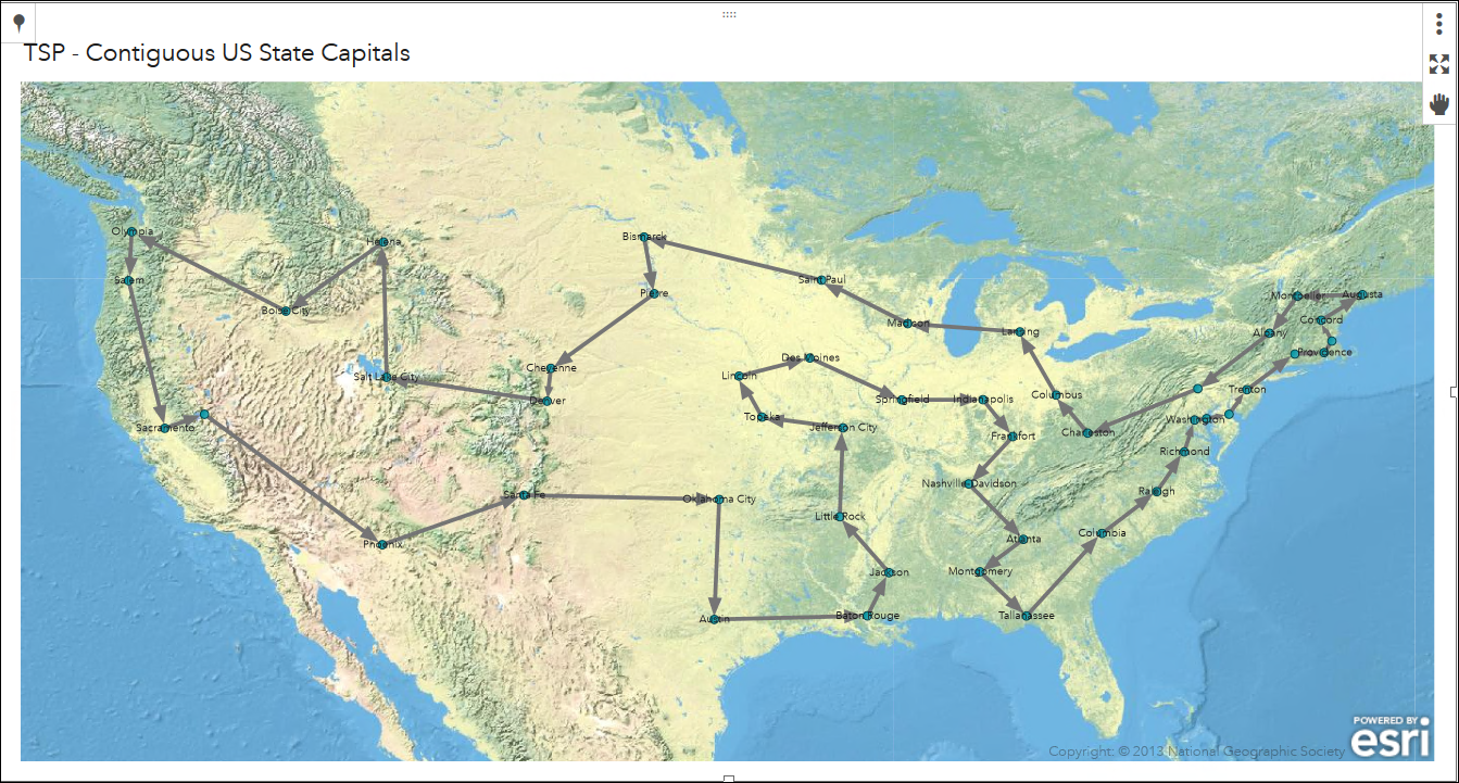 ^[PatriciaNeri, August 2018 https://communities.sas.com/t5/SAS-Communities-Library/What-is-the-shortest-tour-that-visits-only-once-the-48/ta-p/490231]
In this problem, it is easy to get overwhelmed by all of the possibilities. Since there are 49 cities to visit, there are over 6.2*10^60 possibilities. For reference, 10^12 is equivalent to one trillion! Thus, we need an algorithmic approach to solve this problem as opposed to a brute force method.
This page is the main page for Heaps and Priority Queues
The next data structure we will cover is heaps. The heaps discussed in this course are not to be confused with heaps which refer to garbage collection in certain coding languages. Heaps are good for situations were we will need to frequently access and update the highest (or lowest) priority item in a set. For example, heaps are a good data structure to use in Prim’s algorithm. In Prim’s algorithm, we repeatedly got the smallest edge, removed the smallest edge, and then added to and sorted the list of edges.
A heap is an array which we can view as an unsorted binary tree. This tree must have the following properties:
i of the tree, then level i-1 is full. Below we have an example of how this property has been broken. Level two is not full but there are nodes on level three.


As a consequence of the above properties, the following is true as well: Only one node can have one child, all other nodes will have zero or two children. Try to construct a counterexample to see what we mean!
There are two main types of heaps, the max-heap and the min-heap. Depending on the element we want to access we may use one or the other.
A max-heap is a heap such that the parent node is greater than or equal to the children. For example, if we are using a heap to track work flow,we would want to use a max-heap. In this case, the highest priority element will always be the root of the tree.
A min-heap is a heap such that the parent node is less than or equal to the children. This is the opposite of the max-heap. The root of this heap will be the item with the lowest priority. A min-heap may feel unnatural at first, however, this is ideal for greedy algorithms such as Prim’s algorithm. We are frequently getting the smallest edge.
Heaps can be viewed in two forms: as a tree or as an array. We will use the array style in code but we can have the tree structure in the back of our mind to help understand the order of the data. Here is an example of the heap as a tree on the left and the heap as an array on the right.
 The root of the heap will always be the first element. Then we can base the numbering of the following nodes from left to right and top to bottom. For example, the left child of the root will be the second entry and the right child will be the third.
For full functionality of our heap, we want to be able to easily determine the parent of a node as well as the children of a node.
Critical Thinking
Using just the array, how can we determine the parent of a node? In the example above, how can we determine the parent of the node with value 18?
We can formulate the relationships between parent and children nodes mathematically. For a node at index i, we can say that the left child of i will be at index 2i and the right child will be at 2i+1. Similarly, we can say that the parent of node i will be at index floor(i/2).
The function floor(x) like in floor(i/2) will round decimal values down to the next whole number. Some examples:
floor(3.2)=3floor(1.9999)=1floor(4)=4
| Node | Parent | Left Child | Right Child |
|---|---|---|---|
i |
floor(i/2) |
2i |
2i + 1 |
| 1 | N/A | 2*1=2 |
2*1+1=3 |
| 2 | floor(2/2)=1 |
2*2=4 |
2*2+1=5 |
| 3 | floor(3/2)=1 |
2*3=6 |
2*3+1=7 |
| 4 | floor(4/2)=2 |
2*4=8 |
2*4+1=9 |
| 5 | floor(5/2)=2 |
2*5=10 |
2*5+1=11 |
| Try it! |
Consider the following example and try to work some out for yourself.

For example, if we ask for the parent of the node with value 27, our answer would be the node with value 35 The node with value 27 has index 5. Thus, the parent of that node will have index floor(5/2)=2. Node 35 is at index two, as such, node 35 is the parent of node 27.
In a heap where n is the size of heap, the elements floor(n/2)+1 through n will always be leaves. If we assume that we have just the 12 elements in this example, then based on this formula, elements 7 through 12 must be leaves. We can verify this in the tree representation!
A natural implementation of heaps is priority queues.
A priority queue is a data structure which contains elements and each element has an associated key value. The key for an element corresponds to its importance. In real world applications, these can be used for prioritizing work tickets, emails, and much more.

We can use a heap to organize this data for us.

As with heaps, we can have min-priority queues and max-priority queues. For the applications listed above, a max-priority queue is the most intuitive choice. For this course however, we will focus more on min-priority queues which will give us better functionality for greedy algorithms, like Prim’s algorithm.
For the minimum spanning tree algorithms, using a min-priority queue helps the performance of the algorithms. Recall Prim’s algorithm, shown below. Each time we visited a new node, we would add the outgoing edges to the list of available edges, remove the smallest edge, and sort the list.
function PRIM(GRAPH, SRC)
    MST = GRAPH without the edges attribute(s)
    VISITED = empty set
    add SRC to VISITED
    AVAILEDGES = list of edges where SRC is the source
    sort AVAILEDGES
    while VISITED is not all of the nodes
        SMLEDGE = smallest edge in AVAILEDGES
        SRC = source of SMLEDGE
        TAR = target of SMLEDGE
        if TAR not in VISITED
            add SMLEDGE to MST as undirected edge
            add TAR to VISITED
            add the edges where TAR is the source to AVAILEDGES
        remove SMLEDGE from AVAILEDGES
        sort AVAILEDGES
    return MST
If we implement Prim’s algorithm with min-priority queue, we don’t have to worry about sorting the edges every time we add or remove one.
function PRIM(GRAPH, SRC)
    MST = GRAPH without the edges attribute(s)
    VISITED = empty set
    add SRC to VISITED
    AVAILEDGES = min-PQ of edges where SRC is the source
    while VISITED is not all of the nodes
        SMLEDGE = smallest edge in AVAILEDGES
        SRC = source of SMLEDGE
        TAR = target of SMLEDGE
        if TAR not in VISITED
            add SMLEDGE to MST as undirected edge
            add TAR to VISITED
            add the edges where TAR is the source to AVAILEDGES
        remove SMLEDGE from AVAILEDGES
    return MST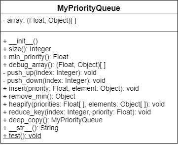
The priority queue will have a single attribute which will be the array to represent the priority queue as a heap. Elements of this array will be ordered pairs where the first entry is the priority and the second entry is the node item.
Since arrays start at index zero, we will set the first element equal to a null value and the element at index 1 will be the start of our priority queue.

Similar to graphs, heaps will have a size which will be the number of elements currently in our heap.
The PUSHDOWN and PUSHUP functions will help us to maintain the heap structure. In their own ways, described below, they will correct the ordering of nodes. Primarily making it such that the parent is always smaller then its children. Both of these will be recursive functions.
PUSHUP: This function takes an index as input and then determines if the element at that index has a lower priority than its parent. This will ‘raise’ the element up through heap and move it closer to the front of the array.
PUSHUP. The first is if the element has greater priority than its parent, then we do nothing as the structure is correct. The second is if the index of the parent node is 0, then we do nothing as we have reached the root of the heap.PUSHUP function with the parent index as input.PUSHDOWN: Similar to PUSHUP this function will take an index as input but will now determine if the node has higher priority than one of its children. This will ’trickle’ the element down through the heap and move it closer to the end of the array.
PUSHDOWN. The first is if the the parent has lower priority than both of its children, then we do nothing as the structure is correct. The second is if the index of both children are out of the range of our array, then we do nothing as we have reached a leaf.This will remove the lowest priority element from our priority queue. If our priority queue only has one element, then we will just remove the element. However, if there is more than the single element, we will need to do some maintenance to make sure the lowest priority element is the root again. To do this, we will take the last element of the priority queue and make it the root. Then we will use the PUSHDOWN function to reorder the nodes.
The HEAPIFY function will allow us to translate our data into a heap. It will take as input a list of priorities and a list of items. Suppose in the figure below, we are calling Prim’s function from node 1. Thus, we want to start our heap with the outgoing edges of node 1. We will input the list of priorities, which in this case are the edge weights, and the list of the items. For this application, we have made the items ordered pairs where the first entry is the source node and the second is the target.

Since we are working primarily with min-priority queues, we will define HEAPIFY in those terms. Though, we could have an equivalent function for a max-priority queue.
For input, the function takes RANKS which is the array representation of our priority values and ITEMS which is the array representation of the items.
function HEAPIFY(RANKS, ITEMS)
    if RANKS and ITEMS are the same size
        SIZE = length of ITEMS
        loop INDEX starting at 1 to SIZE
            I_RANK = value at INDEX in RANKS
            I_ITEM = item at INDEX of ITEMS
            append (I_RANK, I_ITEM) to priority queues array
        QSIZE = length of our PQ - 1
        LASTPARENT = floor(QSIZE/2) + 1
        loop NODE starting at LASTPARENT down to 1
            PUSHDOWN(NODE)
    else
errorThe INSERT function is similar to HEAPIFY but now we are just wanting to insert a single element. As such, INSERT will take the priority of the element and the element as input. We will append the ordered pair of (priority, element) to our priority queue array and then call the PUSHUP function on the last element of the array.
The DECREASEKEY function allows us to update the priority of an element. It takes as input the array index for heap entry to update as well as the priority we will be giving the element. We first check if that the new priority is in fact less than the original. Then we update the priority and then push the element up.
DECREASEKEY(IDX, PRIORITY)
    ELEMENT = entry in array at IDX
    if PRIORITY > ELEMENT[0]
        error
    ELEMENT[0] = PRIORITY
    PUSHUP(IDX)
A good application of priority queues is finding the shortest path in a graph. A common algorithm for this is Dijkstra’s algorithm.
Edsger Dijkstra was a Dutch computer scientist who researched many fields. He is credited for his work in physics, programming, software engineering, and as a systems scientist. His motivation for this algorithm in particular was to be able to find the shortest path between two cities.
“What is the shortest way to travel from Rotterdam to Groningen, in general: from given city to given city? It is the algorithm for the shortest path, which I designed in about twenty minutes. One morning I was shopping in Amsterdam with my young fiancée, and tired, we sat down on the café terrace to drink a cup of coffee and I was just thinking about whether I could do this, and I then designed the algorithm for the shortest path.” - Edsger Dijkstra, Communications of the ACM 53 (8), 2001.
His original algorithm was defined for a path between two specific cities. Since its publication, modifications have been made to the algorithm to find the shortest path to every node given a source node.
DIJKSTRAS(GRAPH, SRC)
    SIZE = size of GRAPH
    DISTS = array with length equal to SIZE
    PREVIOUS = array with length equal to SIZE
    set all of the entries in PREVIOUS to none
    set all of the entries in DISTS to infinity

    DISTS[SRC] = 0
    PQ = min-priority queue

    loop IDX starting at 0 up to SIZE
        insert (DISTS[IDX],IDX) into PQ

    while PQ is not empty
        MIN = REMOVE-MIN from PQ
        for NODE in neighbors of MIN
            WEIGHT = graph weight between MIN and NODE
            CALC = DISTS[MIN] + WEIGHT
            if CALC < DISTS[NODE]
                DISTS[NODE] = CALC
                PREVIOUS[NODE] = MIN
                PQIDX = index of NODE in PQ
                PQ decrease-key (PQIDX, CALC)
    return DISTS and PREVIOUS
^[Shiyu Ji, CC BY-SA 4.0 https://creativecommons.org/licenses/by-sa/4.0, via Wikimedia Commons, https://upload.wikimedia.org/wikipedia/commons/e/e4/DijkstraDemo.gif]
Aside from just finding routes for us to travel, Dijkstra’s algorithm can accommodate for any application that can have an abstraction to finding the shortest path. For example, the following animation shows how a robot could utilize Dijkstra’s algorithm to find the shortest path with an obstacle in the way. In this example, each node could represent one square foot of floor space and the edges would represent those spaces that are adjacent. In this scenario, we would most likely not have an associated edge weight. If the robot were traversing on a rugged terrain, then we could have the weights represent the difficultly of passing through the terrain from one space to the other.
 ^[Subh83, CC BY 3.0 https://creativecommons.org/licenses/by/3.0, via Wikimedia Commons, https://commons.wikimedia.org/wiki/File:Dijkstras_progress_animation.gif]
Another practical abstraction is in network routing. In this simplified abstraction, nodes would be routers or switches and the edges would be the physical links between them. The edge weights in this case would be the cost of sending a packet from one router to the next. Dijkstra’s algorithm is actively used in protocols such as Intermediate System to Intermediate System (IS-IS) and Open Shortest Path First (OSPF).
This page is the main page for Performance
In this module, we will reintroduce the data structures that we have seen and implemented throughout CC315 as well as CC310. We will discuss the running time for various operations as well as space requirements for each structure.
You may recall that in CC310, we did a similar comparison. We will use most of the same operations from that module so we can draw comparisons between the structures in CC310 and CC315.
We will also also discuss the memory required for each structure.
There are three types of trees to consider: generic trees, tries, and binary trees.

Insert: In general, inserting an element into a tree by making it a child of an existing tree is a constant time operation. However, this depends on us already having access to the parent tree we’d like to add the item to, which may require searching for that element in the tree as discussed below, which runs in linear time based on the size of the tree. As we saw in our projects, one way we can simplify this is using a hash table to help us keep track of the tree nodes while we build the tree, so that we can more quickly access a desired tree (in near constant time) and add a new child to that tree.
Access: Again, this is a bit complex, as it requires us to make some assumptions about what information is available to us. Typically, we can only access the root element of a tree, which can be done in constant time. If we’d like to access any of the other nodes in the tree, we’ll have to traverse the tree to find them, either by searching for them if we don’t know the path to the item (which is linear time based on the size of the tree), or directly walking the tree in the case that we do know the path (which is comparable to the length of the path, or linear based on the height of the tree).
Find: Finding a particular node in a generic tree is a linear time operation based on the number of nodes in the tree. We simply must do a full traversal of the tree until we find the element we are searching for, typically either by performing a preorder or postorder traversal. This is very similar to simply looking at each element in a linear data structure.
Delete: Removing a child from an existing tree is an interesting operation. If we’ve already located the tree node that is the parent of the element we’d like to remove, and we know which child we’d like to remove, then the operation would be a linear time operation related to the number of children of that node. This is because we may have to iterate through the children of that tree node in order to find the one we’d like to remove. Recall that trees generally store the children of each node in a linked list or an array, so the time it takes to remove a child is similar to the time it takes to remove an element from those structures. Again, if we have to search for either the parent or the tree node we’d like to remove from that parent, we’ll have to take that into account.
Memory: In terms of memory usage, a generic tree uses memory that is on the order of the number of nodes in the tree. So, as the number of nodes in the tree is doubled, the amount of memory it uses doubles as well.

Tries improve on the structure of trees in one important way - instead of using a generic list to store each child, they typically use a statically sized array, where each index in the array directly corresponds to one of the possible children that the node could have. In the case of a trie that represents words, each tree node may have an array of 26 possible children, one for each letter of the alphabet. In our implementation, we chose to use lists instead to simplify things a bit, but for this analysis we’ll assume that the children of a trie node can be accessed in constant time through the use of these static arrays.
In the analysis below, we’ll assume that we are dealing with words in a trie, not individual nodes. We’re also going to be always starting with the root node of the overall trie data structure.
Insert: To insert a new word in a trie, the process will run in linear time based on the length of the word. So, to insert a 10 character word in a trie, it should take on the order of 10 steps. This is because we can find each individual node for each character in constant time since we are using arrays as described above, and we’ll need to do that once for each character, so the overall time is linear based on the number of characters. If the path doesn’t exist, we’ll have to create new tree nodes to fill it in, but if the path does exist, it could be as simple as setting the boolean value at the correct node to indicate that it is indeed a word.
Access: Similarly to determine if a particular word is in the trie, it will also run in linear time based on the length of the word. We simply must traverse through the path in the tree, and at each node it is a constant time operation to find the correct child and continue onward. So, in total this is a linear time operation.
Find: Find is pretty much the same as access, since we can’t just directly jump to a particular node in the tree. So, this is also in linear time based on the length of the word.
Delete: Once again, deleting a word simply involves finding it, which runs in linear time. Once it is deleted, we may go through and prune branches that are unused, which is also a linear time operation as we work back upwards in the trie. So, overall the whole operation runs in linear time based on the length of the word.
In summary, pretty much every operation performed on a trie is related to the length of the word that is provided as input. Pretty nifty!

A binary tree is a tree that is limited to having only two children of each node, and the children and parents are sorted such that every element to the left of the node is less than or equal to its value, and all elements to the right of the node are greater than or equal to its value. Because of this, they perform a little differently than traditional trees.
One major concept related to binary trees is whether the tree is “balanced” or not. A balanced tree has children that differ in height by no more than 1. If the tree is perfectly balanced, meaning all subtrees are balanced, then there are some interesting relationships that develop.
Most notably, the overall height $h$ of the tree is no larger than $log_2(n)$, where $n$ is the number of elements in the tree.
We didn’t cover the algorithms to balance a binary tree in this course since they can be a bit complex, but for this analysis we’ll discuss the performance of binary trees when they are perfectly balanced as well as when they are unbalanced.
Insert: To insert a new element in a binary tree, we may have to descend all the way to the bottom of the tree, so the operation is linear based on the height of the tree. If the tree is a perfectly balanced binary tree, then it is on the order of $log_2(n)$. Otherwise, it is linear based on the height, which in the worst case of a completely unbalanced tree could be the number of nodes itself. Once you’ve added the new item, a perfectly balance tree may need to rebalance itself, but that operation is not any more costly than the insert operation.
Access: Similarly, to access a particular element in a binary tree, we’ll have to descend through the tree until we find the element we are looking for. At each level, we know exactly which child to check, so it is once again related to the height of the tree. If the tree is a perfectly balanced binary tree, then it is on the order of $log_2(n)$. Otherwise, it is linear based on the height, which in the worst case of a completely unbalanced tree could be the number of nodes itself.
Find: Once again, find in this instance is similar to access.
Delete: Finally, deleting an element from a binary tree involves finding the element, which will be linear based on the height of the tree. Once the element is removed, then a perfectly balanced tree will need to rebalance itself, which could also take the same amount of time. So, in both cases, it runs on the order of $h$ time, which in the worst case is the total number of nodes $n$ on an unbalanced tree, or $log_2(n)$ on a perfectly balanced tree.
So, most operations involving a perfectly balanced binary tree run in $log_2(n)$ time, which is very efficient when compared to a generic tree. However, if the tree is not balanced, then we cannot make any assumptions about the height of the tree and each operation could require $n$ time, where $n$ is the number of nodes in the tree.
There are two types of graphs that we’ve covered in this class: list graphs and matrix graphs. Graphs are slightly different than other data structures, because we may want to find or access both nodes and edges in the graph. So, we’ll need to analyze the performance of graphs with respect to both nodes and edges.
Recall that a matrix graph uses an array to store the nodes, and a two-dimensional array to store the edges.
Insert Node: Inserting a node is a linear time operation. To insert node, we looped through the nodes attribute and put the node in the first open index. Thus, it is linear with respect to the number of nodes.
Access Node: Likewise, given the index of a node, we can get it’s value in constant time by accessing the array.
Find Node: To find the index of a node when we are given its value, we must iterate through the array of nodes, which will be a linear time operation based on the number of nodes in the graph.
Delete Node: Finally, to remove a node from a graph we can simply set its value in the array of nodes to null. However, we may also need to go through the list of edges and make sure there are no edges to or from that node, so typically this operation runs on the order of the number of nodes in the graph since we must check each one.
For the operations relating to edges below, we’ll assume that we already know the indices of the two nodes we are connecting. If we don’t know those, we’ll have to use the find node process above first.
Insert Edge: To insert an edge into the graph we simply update the element in the two-dimensional array, which can be done in constant time.
Access Edge: Likewise, to access an edge between two nodes, we simply access the element in the two-dimensional array, which is a constant time operation.
Find Neighbors: Instead of finding a particular edge, we’ll say that we want to find all of the neighboring nodes that can be accessed from a given node. In this case, we’ll need to iterate through one row of the two-dimensional array, so the whole process runs on the order of linear time based on the number of nodes in the graph.
Delete Edge: To remove an edge, we simply find it in the two-dimensional array and set its value to infinity, which can be done in constant time.
So, for most matrix graph operations, we can do nearly everything in either constant time or, at worst, linear time based on the number of nodes in the graph.
Recall that a list graph uses an array to store the nodes, and then each node stores a list of edges that start from that node.
Insert Node: Inserting a node is a linear time operation. To insert node, we looped through the nodes attribute and put the node in the first open index. Thus, it is linear with respect to the number of nodes.
Access Node: Likewise, given the index of a node, we can get it’s value in constant time by accessing the array.
Find Node: To find the index of a node when we are given its value, we must iterate through the array of nodes, which will be a linear time operation based on the number of nodes in the graph.
Delete Node: Finally, to remove a node from a graph we can simply set its value in the array of nodes to null. However, we may also need to go through each other node and check to make sure it isn’t in the list of edges. So typically this operation runs on the order of the number of nodes in the graph since we must check each one.
So far, a list graph seems to be pretty similar to a matrix graph in terms of performance. The real difference comes with how we handle edges, as well see next.
For the operations relating to edges below, we’ll assume that we already know the indices of the two nodes we are connecting. If we don’t know those, we’ll have to use the find node process above first.
Insert Edge: To insert an edge into the graph, we must get the source node from the nodes array and then add an element to the list of edges. Assuming that the edges are stored in a linked list, this is a linear time operation in terms of the number of nodes since we may have to iterate through the list of edges to make sure this edge doesn’t already exist and need updated. In the worst case, there may be $n$ edges here, so it is a linear operation.
Access Edge: To access an edge between two nodes, we first find the source node in the list of nodes, which is a constant time operation. Then, we’ll have to iterate through the list of edges, which is at worst linear time based on the size of the graph, since there could be $n$ outgoing edges from this node. So, overall the operation runs on the order of linear time based on the number of nodes in the graph.
Find Neighbors: Instead of finding a particular edge, we’ll say that we want to find all of the neighboring nodes that can be accessed from a given node. In this case, we can just find the source node in the array of nodes, which is a constant time operation. Then, we can simply return the list of edges, which is also constant time. So, this operation is very efficient!
Delete Edge: To remove an edge, we find the source node and iterate through the list of edges until we find the one to remove. So, this runs in linear time based on the number of nodes in the graph.
So, for most list graph operations, we can also do nearly everything in either constant time or, at worst, linear time based on the number of nodes in the graph. The only real difference comes in how we handle edges, where some operations are a bit slower, but getting a list of all the neighbors of a node is actually a little quicker!
Let’s analyze the memory usage of matrix and list graphs when dealing with dense and sparse graphs. This is the real key difference between the two data structures.
A dense graph is a graph that has a large number of edges compared to the maximum number of edges possible. More specifically, the maximum number of edges a graph can have is $n^2$, so we would say a dense graph has a value for $e$ that is close to $n^2$. Because of this, the memory usage of a matrix graph ($n^2$) is actually a bit more efficient than a list graph ($n + n^2$) because it doesn’t have the extra overhead of maintaining a list structure for each node.
A sparse graph is a graph that has a small number of edges compared to the maximum number of edges possible. So, here we would say that the value of $e$ is much smaller than $n^2$, though it may still be larger than $n$ (otherwise each node would only have one edge coming from it, and this would be a linked list). In that case, we see that $n + e$ is much smaller than $n^2$, and a list graph is much more efficient. If you think about it, in a matrix graph a large number of the entries in the two-dimensional array would be set to infinity and unused, but they still take up memory. Those unused edges wouldn’t exist in a list graph, making it much more memory efficient.
Let’s look at the performance of priority queues next. These structures are based on a heap, which has some unique characteristics related to the heap properties that it must maintain.
Recall that a heap is an array which we can view as an unsorted binary tree. This tree must have the following properties:
i of the tree, then level i-1 is full.Insert To insert a new element in a priority queue, we place it at the end and then push it upwards until it is in the correct place. Because the heap property creates a perfectly balanced tree, at most it will have to perform $log_2(n)$ or $h$ operations. So, we say that insert runs on the order of $log_2(n)$ where $n$ is the number of elements in the heap.
Access Minimum The most common operation for accessing elements in the priority queue is to access the minimum element. Since it should always be the first element in the array due to the heap properties, this is clearly a constant time operation.
Find Element To find an item in a priority queue, we must simply iterate through the array that stores the heap, which is a linear time operation based on the number of elements in the heap.
Remove Minimum To remove the smallest element, we swap it with the last element and then remove it, then push the top element down into place. Similar to the push up operation, at most it will perform $log_2(n)$ or $h$ operations. So, we say that remove minimum runs on the order of $log_2(n)$ where $n$ is the number of elements in the heap.
Heapify This is the most interesting operation of a heap. When we use heapify, we add a large number of elements to the heap and then sort it exactly once by working from the bottom to the top and pushing down each element into place. On the surface, it appears that this should run in the order $n * log_2(n)$ time, since each push down operation takes $log_2(n)$ time, and we have to do that on the order of $n$ times to get each element in place. However, using a bit of mathematical analysis, it is possible to prove that this operation actually runs in linear time $n$ based on the number of elements. The work to actually prove this is a bit beyond the scope of this course, but this StackOverflow discussion is a great explanation of how it works.
Memory: In terms of memory usage, a priority queue uses memory that is on the order of the number of elements in the priority queue.
Why is it important that heapify runs in linear time? That is because we can use heapify and remove minimum to sort data, which is a sorting algorithm known as heap sort.
We already saw that heapify runs in linear time based on the number of nodes, and each remove minimum operation runs in $log_2(n)$ time. To remove all the elements of the heap, we would do that $n$ times, so the overall time would be $n * log_2(n)$ time. If you recall, that is the same performance as merge sort and quicksort!
This page will be devoted to summarizing our performance discussions. Below, we have included a graph for a frame of reference for the various functions.
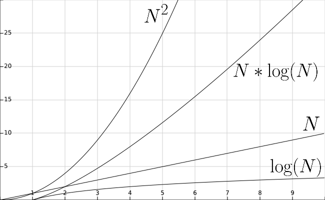
In the following, $n$ denotes the number of nodes in the tree.
In the following, $m$ denotes the length of a word and $n$ denotes the number of words in the trie.
In the following, $n$ denotes the number of nodes in the tree.
In the following, $n$ denotes the number of nodes in the graph.
In the following, $n$ denotes the number of nodes in the graph and $e$ denotes the number of edges.
In the following, $n$ denotes the number of elements in the priority queue.
We will now discuss the performance of the algorithms that we discussed in this course. When examining the performance of an algorithm we will look at the time and the space that it will require.
function PREORDER(RESULT)
    append ITEM to RESULT
    FOR CHILD in CHILDREN
           CHILD.PREORDER(RESULT)
end function
function POSTORDER(RESULT)
FOR CHILD in CHILDREN
CHILD.POSTORDER(RESULT)
append ITEM to RESULT
end functionRESULT is a variable defined and stored outside of the algorithm, it does not factor into our space requirement. Then we must account for the variables CHILD and CHILDREN. In any given iteration, CHILD will be constant and CHILDREN will have size equal to the number of children for the node we are currently at. In total, this would give us a space requirement that is linear with respect to the number of nodes.function INORDER(RESULT)
LEFTCHILD.INORDER(RESULT)
append ITEM to RESULT
RIGHTCHILD.INORDER(RESULT)
end functionRESULT is a variable defined and stored outside of the algorithm, it does not factor into our space requirement. Then we must account for the variable ITEM. This will have constant space and thus, the space requirement for the inorder traversal is constant.1. function DEPTHFIRSTSEARCH(GRAPH,SRC,TAR)
2. STACK = empty array
3. DISCOVERED = empty set
4. PARENT_MAP = empty dictionary
5. append SRC to STACK
6. while STACK is not empty
7. CURR = top of the stack
8. if CURR not in DISCOVERED
9. if CURR is TAR
10. PATH = empty array
11. TRACE = TAR
12. while TRACE is not SRC
13. append TRACE to PATH
14. set TRACE equal to PARENT_MAP[TRACE]
15. reverse the order of PATH
16. return PATH
17. add CURR to DISCOVERED
18. NEIGHS = neighbors of CURR
19. for EDGE in NEIGHS
20. NODE = first entry in EDGE
21. append NODE to STACK
22. if PARENT_MAP does not have key NODE
23. in the PARENT_MAP dictionary set key NODE with value CURR
24. return nothingSTACK can contain duplicates. In the case that we have a sparse graph, this would be bound by the number of nodes. For a dense graph however, the number of executions would be bound by the number of edges. The code within the while loop would be bound by the number of nodes because of the check that we have not already discovered the node in line 8. If we haven’t discovered it, we would take either the logic of lines 8 through 16 or lines 17 through 23 but never both in the same iteration. Both of these blocks are bound by the number of nodes in our graph. Thus the worst case time requirement would be $n^2$.STACK can contain duplicate nodes. If we have a sparse graph then it will be bound by the number of nodes. If we have a dense graph then the space is bound by the number of edges.
STACK: linear with respect to the number of edgesDISCOVERED: linear with respect to the number of nodesPARENT_MAP: linear with respect to the number of nodesCURR: 1PATH: linear with respect to the number of nodesTRACE: 1NEIGHS: linear with respect to the number of neighborsEDGE: 1NODE: 11. function BREADTHFIRSTSEARCH(GRAPH,SRC,TAR)
2. QUEUE = empty queue
3. DISCOVERED = empty set
4. PARENT_MAP = empty dictionary
5. add SRC to DISCOVERED
6. add SRC to QUEUE
7. while QUEUE is not empty
8. CURR = first element in QUEUE
9. if CURR is TAR
10. PATH = empty list
11. TRACE = TAR
12. while TRACE is not SRC
13. append TRACE to PATH
14. set TRACE equal to PARENT_MAP[TRACE]
15. reverse the order of PATH
16. return PATH
17. NEIGHS = neighbors of CURR
18. for EDGE in NEIGHS
19. NODE = first entry in EDGE
20. if NODE is not in DISCOVERED
21. add NODE to DISCOVERED
22. if PARENT_MAP does not have key NODE
23. in the PARENT_MAP dictionary set key NODE with value CURR
24. append NODE to QUEUE
25. return nothingQUEUE will never have duplicates. Lines 1 through 6 will all execute in constant time. The while loop will occur $n$ times where $n$ is the number of nodes. Based on the logic, either 9-16 will execute or 17-24 will execute. Both of these are bound by the number of nodes in terms of time. Each iteration of the while loop will take $n$ time and we do the while loop $n$ times; thus the running time will be $n^2$.QUEUE: linear with respect to the number of nodesDISCOVERED: linear with respect to the number of nodesPARENT_MAP: linear with respect to the number of nodesCURR: 1PATH: linear with respect to the number of nodesTRACE: 1NEIGHS: linear with respect to the number of nodesEDGE: 1NODE: 11. function KRUSKAL(GRAPH)
2. MST = GRAPH without the edges attribute(s)
3. ALLSETS = an empty list which will contain the sets
4. for NODE in GRAPH NODES
5. SET = a set with element NODE
6. add SET to ALLSETS
7. EDGES = list of GRAPH's edges
8. SORTEDEDGES = EDGES sorted by edge weight, smallest to largest
9. for EDGE in SORTEDEDGES
10. SRC = source node of EDGE
11. TAR = target node of EDGE
12. SRCSET = the set from SETS in which SRC is contained
13. TARSET = the set form SETS in which TAR is contained
14. if SRCSET not equal TARSET
15. UNIONSET = SRCSET union TARSET
16. add UNIONSET to ALLSETS
17. remove SRCSET from ALLSETS
18. remove TARSET from ALLSETS
19. add EDGE to MST as undirected edge
20. return MSTTime: The time to initialize MST would be linear with respect to the number of nodes. Regardless of the graph implementation, inserting nodes is constant time and we would do it for the number of nodes in GRAPH. Lines 4-6 would take linear time with respect to the number of nodes. Then lines 9-19 would take linear time with respect to the number of edges as it would execute $e$ times and each operation can be done in constant time, except for searching through the sets and performing set operations, which require $log_2(n)$ time. Thus, Kruskal’s algorithm will take time on the order of $e \times log_2(n)$ in the worst case.
Space:The required space for Kruskal’s algorithm is dependent on the implementation of the MST. A matrix graph would require $n^2$ space and a list graph we would require $n+e$ space.
MST: matrix graph $n^2$ or list graph $n+e$ALLSETS: linear with respect to the number of nodesNODE: 1GRAPH NODES: linear with respect to the number of nodesSET: 1EDGES: linear with respect to the number of edgesSORTEDEDGES: linear with respect to the number of edgesSRC: 1TAR: 1SRCSET: 1TARSET: 1UNIONSET: 11. function PRIM(GRAPH, START)
2. MST = GRAPH without the edges attribute(s)
3. VISITED = empty set
4. add START to VISITED
5. AVAILEDGES = list of edges where START is the source
6. sort AVAILEDGES
7. while VISITED is not all of the nodes
8. SMLEDGE = smallest edge in AVAILEDGES
9. SRC = source of SMLEDGE
10. TAR = target of SMLEDGE
11. if TAR not in VISITED
12. add SMLEDGE to MST as undirected edge
13. add TAR to VISITED
14. add the edges where TAR is the source to AVAILEDGES
15. remove SMLEDGE from AVAILEDGES
16. sort AVAILEDGES
17. return MSTMST would be linear with respect to the number of nodes. Regardless of the graph implementation, inserting nodes is constant time and we would do it for the number of nodes in GRAPH. With a matrix graph, setting up AVAILEDGES would take linear time with respect to the number of nodes. With a list graph, this would happen in constant time. Then, we need to get the smallest edge from the AVAILEDGES list, which would be a linear time operation based on the number of edges, and we must do that once for up to each edge in the graph. So, the worst case running time for Prim’s algorithm is $e^2$. (Our implementation is actually a bit slower than this since we sort the list of available edges each time, but that is technically not necessary - our implementation is closer to $e^2 \times log_2(e)$!)MST: matrix graph $n^2$ or list graph $n+e$VISITED: linear with respect to the number of nodesAVAILEDGES: linear with respect to the number of edgesSMLEDGE: 1SRC: 1TAR: 11. DIJKSTRAS(GRAPH, SRC)
2. SIZE = size of GRAPH
3. DISTS = array with length equal to SIZE
4. PREVIOUS = array with length equal to SIZE
5. set all of the entries in PREVIOUS to none
6. set all of the entries in DISTS to infinity
7. DISTS[SRC] = 0
8. PQ = min-priority queue
9. loop IDX starting at 0 up to SIZE
10. insert (DISTS[IDX],IDX) into PQ
11. while PQ is not empty
12. MIN = REMOVE-MIN from PQ
13. for NODE in neighbors of MIN
14. WEIGHT = graph weight between MIN and NODE
15. CALC = DISTS[MIN] + WEIGHT
16. if CALC < DISTS[NODE]
17. DISTS[NODE] = CALC
18. PREVIOUS[NODE] = MIN
19. PQIDX = index of NODE in PQ
20. PQ decrease-key (PQIDX, CALC)
21. return DISTS and PREVIOUSPQ is not empty (line 11), which is bound by the number of nodes. Thus, the block of code starting at 11 will take $n^2$ time to run in the worst case. This means that if we double the number of nodes, then the running time will be quadrupled. The worst case for Dijkstra’s algorithm is characterized by being a very dense graph, meaning each node has a lot of neighbors. If the graph is sparse and our priority queue is efficient, we could expect this running time to be more along the lines of $(n + e) \times log_2(n)$, where $e$ is the number of edges.SIZE: 1DISTS: linear with respect to the number of nodesPREVIOUS: linear with respect to the number of nodesPQ: linear with respect to the number of nodesIDX: 1MIN: 1NODE: 1NEIGHBORS: linear with respect to the number of nodesWEIGHT: 1CALC: 1PQIDX: 1A stack is a data structure with two main operations that are simple in concept. One is the push operation that lets you put data into the data structure and the other is the pop operation that lets you get data out of the structure.
A stack is what we call a Last In First Out (LIFO) data structure. That means that when we pop a piece of data off the stack, we get the last piece of data we put on the stack.
A queue data structure organizes data in a First In, First Out (FIFO) order: the first piece of data put into the queue is the first piece of data available to remove from the queue.
A list is a data structure that holds a sequence of data, such as the shopping list shown below. Each list has a head item and a tail item, with all other items placed linearly between the head and the tail.
A set is a collection of elements that are usually related to each other.
A hash table is an unordered collection of key-value pairs, where each key is unique.
The following table compares the best- and worst-case processing time for many common data structures and operations, expressed in terms of $N$, the number of elements in the structure.
| Data Structure | Insert Best | Insert Worst | Access Best | Access Worst | Find Best | Find Worst | Delete Best | Delete Worst |
|---|---|---|---|---|---|---|---|---|
| Unsorted Array | $1$ | $1$ | $1$ | $1$ | $N$ | $N$ | $N$ | $N$ |
| Sorted Array | $\text{lg}(N)$ | $N$ | $1$ | $1$ | $\text{lg}(N)$ | $\text{lg}(N)$ | $\text{lg}(N)$ | $N$ |
| Array Stack (LIFO) | $1$ | $1$ | $1$ | $1$ | $N$ | $N$ | $1$ | $1$ |
| Array Queue (FIFO) | $1$ | $1$ | $1$ | $1$ | $N$ | $N$ | $1$ | $1$ |
| Unsorted Linked List | $1$ | $1$ | $N$ | $N$ | $N$ | $N$ | $N$ | $N$ |
| Sorted Linked List | $N$ | $N$ | $N$ | $N$ | $N$ | $N$ | $N$ | $N$ |
| Linked List Stack (LIFO) | $1$ | $1$ | $1$ | $1$ | $N$ | $N$ | $1$ | $1$ |
| Linked List Queue (FIFO) | $1$ | $1$ | $1$ | $1$ | $N$ | $N$ | $1$ | $1$ |
| Hash Table | $1$ | $N$ | $1$ | $N$ | $N$ | $N$ | $1$ | $N$ |
This page is the main page for Requirements Analysis
In this module, we will discuss how we can determine which data structure we should choose when storing real-world data. We’ll typically make this decision based on the characteristics of the data we would like to store. In general, the data structures we’ve learned often work together well and complement each other, as we saw in Dijkstra’s algorithm. In some cases, one structure can be utilized to implement another, such as using a linked list to implement a stack or a queue.
When selecting a data structure for a particular data set, there are a few considerations we should keep in mind.
The first consideration is: does this data structure work for our data? To answer this, we would want to the characteristics in the data and then determine if our chosen data structure:
Once we have chosen a possible data structure, we also must consider if the choice clearly makes sense to another person who reviews our work. Some questions we may want to ask:
Finally, we should always consider the performance of our program when selecting a data structure. In some cases, the most straightforward data structure may not always be the most efficient, so at times there is a trade off between performance and simplicity. Consider the hash table structure - it may seem like a more complicated array or linked list. But, if we need to find a specific item in the structure, a hash table is typically much faster due to the use of hashes. That increase in complexity pays off in faster performance. So, when analyzing data structures for performance, we typically look at these things:
We will address this particular facet in the next chapter. For now, we will focus on the first two portions.
The first step toward determining which data structure to use relies heavily on the format of the data. By looking at the data and trying to understand what it contains and how it works, we can get a better idea of what data structure would work best to represent the data. Here, we will discuss some main types of data that we could encounter.
Unique data is the type of data where each element in a group must be unique - there can be no duplicates. However, in many cases the data itself doesn’t have a sequence or fixed ordering, we simply care if an element is present in the group or not. Some examples of unique data:
This data is best stored in the set data structure, usually built using a hash table as we learned previously.
However, many times this data may be included along with other data (a person’s ID number is part of the person’s record), so sets are rarely used in practice. Instead, we can simply modify other data structures to enforce the uniqueness property we desire on those attributes. In addition, we see this concept come up again in relational databases, where particular attributes can be assigned a property to enforce the rule that each element must be unique.
Linear data refers to data that has a sequence or fixed ordering. This can include
This data is typically stored in the array or linked list data structure, depending on how we intend to use it and what algorithms will be performed on the data.
We can think of this type of data as precisely one after another. This means that from one element there will be exactly one “next” element.
Finally, we can also adapt these data structures to represent FIFO (first-in, first-out) and LIFO (last-in, first-out) data structures using queues and stacks. As we saw previously, most implementations of queues and stacks are simply adaptations of existing linear data structures, usually the linked list.
Associative data is data where a key is associated with a value, usually in order to quickly find and retrieve the value based on its key. Some examples are:
We typically use a hash table to store this data in our programs.
However, in many cases this data could also be stored in a relational database just as easily, and in most industry programs that may also be a good choice here. Since we haven’t yet learned about relational databases, we’ll just continue to use hash tables for now.
Hierarchical data refers to data where elements can be seen as above, below, or on the same level as other elements. This can include
In contrast to linear data, hierarchical data can have multiple elements following a single element. In hierarchical data, each element has exactly one element prior to it. We typically use some form of a tree data structure to store hierarchical data.
Relational data refers to data where elements are ‘close to’ or ‘far from’ other elements. We can also think of this as ‘more similar’ and ’less similar’ as well. This can include
In a relational data set, any element can be ‘related’ to any other element. We typically use a graph data structure to store relational data.
The last type of data we will discuss is prioritized data. Here, we want to store a data element along with a priority, and then be able to quickly retrieve the element with the highest or lowest priority, depending on use. This could include:
For this data, we typically use an implementation of a priority queue based on a heap. It is important to remember that the heap does not store the data in sorted order - otherwise we would just use a linear data structure for this. Instead, it guarantees that the next element is always stored at the front of the structure for easy access, and it includes a process to quickly determine the new next element. We’ll learn a bit more about why this is so helpful in the next chapter covering performance.
It is important to note that when we are given a set of requirements for a project, the developer may not use the words to classify the types of data. Based on what a user tells us, we want to be able to infer what kind of shape the data could take.
In general, trees are good for hierarchical data. While trees can be used for linear data, it is inefficient to implement them in that way (from a certain point of view, a linked list is simply a tree where each node can only have one child). When data points have many predecessors, trees cannot be used. Thus, trees are not suitable for most relational data.
To recap, we defined a tree as having the following structure:
In this course, we used trees to represent family lineage and biologic classifications. Once we have the data in a tree, we can perform both preorder and postorder traversals to see all of the data, and we can use the structure of the tree to determine if two elements are related as ancestor and descendant or not.
We added constraints to trees to give us special types of trees, discussed below.
A trie is a type of tree with some special characteristics, which are:
Tries are best suited for data sets in which elements have similar prefixes. In this course we focused on tries to represent words in a language, which is the most common use of tries. We used tries for an auto-complete style application.

Tries are a very efficient way of storing dense hierarchical data, since each node in the trie only stores a single portion of the overall data. They also allow quickly looking up if a particular element or path exists - usually much quicker than looking through a linear list of words.
A binary tree is a type of tree with some special characteristics, which are:
Binary trees are the ideal structure to use when we have a data set with a well defined ordering. Once we have the data stored in a binary tree, we can also do an inorder traversal, which will access the elements in the tree in sorted order. We will discuss in the next chapter why we might want to choose a binary tree based on its performance.
Graphs are a good data structure for relational data. This would include data in which elements can have some sort of similarity or distance defined between those elements. This measure of similarity between elements can be defined as realistically or abstractly as needed for the data set. The distance can be as simple as listing neighbors or adjacent elements.
Graphs are multidimensional data structures that can represent many different types of data using nodes and edges. We can have graphs that are weighted and/or directed and we have introduced two ways we can represent graphs:
The first implementation of graphs that we looked at were matrix graphs. In this implementation, we had an array for the nodes and a two dimensional array for all of the possible edges.
The second implementation of graphs were list graphs. For this implementation, we had a single array of graph node objects where the graph node objects tracked their own edges.
Recall that we discussed sparse and dense graphs. Matrix graphs are better for dense graphs since a majority of the elements in the two dimensional array of edges will be filled. A great example of a dense graph would be relationships in a small community, where each person is connected to each other person in some way.
List graphs are better for sparse graphs, since each node only needs to store the outgoing edges it is connected to. This eliminates a large amount of the overhead that would be present in a matrix graph if there were thousands of nodes and each node was only connected to a few other nodes. A great example of a sparse graph would be a larger social network such as Facebook. Facebook has over a billion users, but each user has on average only a few hundred connections. So, it is much easier to store a list of those few hundred connections instead of a two dimensional matrix that has over one quintillion ($10^{18}$) elements.
In the next chapter, we will discuss the specific implications of using one or the other. However, in our requirement analysis it is important to take this into consideration. If we have relational data where many elements are considered to be connected to many other elements, then a matrix graph will be preferred. If the elements of our data set are infrequently connected, then a list graph is the better choice.
The last structure we covered were priority queues. On their own, these are good for hierarchical data. We discussed using priority queues for ticketing systems where the priority is the cost or urgency. In the project, we utilized priority queues in conjunction with Dijkstra’s algorithm.
A priority queue is a data structure which contains elements and each element has an associated priority value. The priority for an element corresponds to its importance. For this course, we implemented priority queues using heaps.
A key point of priority queues is that the priority for a value can change. This is reflected by nodes moving up (via push up) or down (via push down) through the priority queue.
In contrast, a tree has a generally fixed order. Consider the file tree as a conceptual example, it is not practical for a parent folder to switch places with a child folder.
In real world applications, it won’t always be a straightforward choice to use one structure over another. Users may come to us with unclear ideas of what they are looking for and we will need to be able to infer what structure is best suited for their needs based on what we can learn from them. Typically, those describing applications to us may not be familiar with the nomenclature we use as programmers. Instead, we have to look for clues about how the data is structured and used to help us choose the most appropriate data structures
Below we have some examples with possible solutions. We say possible solutions because there may be other ways that we could implement things. It is important that no matter what structure or algorithm we use, we should always document why we chose our answer. If someone else were to join on the project at a later time, it is important that they understand our reasoning.
A manager at a costume shop has requested that we do some data management for their online catalog. They say:
Take a moment to think on how you might go about this. Remember, there can be multiple ways of solving these problems. We need to be sure that we can articulate and justify our answers.
This is a situation where we could potentially use all three data structures!
First, we could use a tree to represent the search refinement. Thinking along the lines of a data structure, each category and subsequently each product will have exactly one parent. While something like ‘wigs’ shows up in all three categories, you wouldn’t want dog wigs showing up in a search for adult wigs. Thus, there is a unique ancestry for each category and product.

In this scenario we had a fixed ordering of our hierarchy. If the manager wanted users to be able to sort by costume part and then who it was for, our tree would not hold up.
The second portion that was requested was a recommendation system. We could implement this in two parts. The first would be a graph in which the nodes are the products and they are connected based on the similarity of the products.
For example, a purple childrens wig will be very similar to a childrens blue wig but it would be very different from an adults clown shoes. Thus, our graph would have a heavily weighted connection between the childrens purple and blue wig and there would be an edge with a very small weight between the purple wig and adult clown shoes. We can obtain this information from the manager. Since each product will be connected to every other product, a matrix graph would be best suited here.
Then once we have the graph, we could implement a priority queue. The priority queue would be built based off of the users search. When a user searches for a product, we would refer to our graph and get other similar products and enqueue them. The priority would be similarity to the searched products and the item would be the recommended product. As they continue to search, we would dequeue an element if the user selects it and we would change the priority of elements based on commonalities in the searches.
A friend approaches you about their idea for a video game and ask how they could use different data structures to produce the game. They tell us about their game which is a sandbox game with no defined goals. Users can do tasks at their own chosen speed and there is no real “completion” of the game. They say:
Take a moment to think on how you might go about this. Remember, there can be multiple ways of solving these problems. We need to be sure that we can articulate and justify our answers.
Again, this is a situation where we could potentially use three data structures!
We can use a priority queue to suggest tasks for the players to do. In this priority queue, the priority would be the payout and the item would be the task itself. As tasks get completed, we would dequeue them.
We can use a trie to represent the set of shortcuts. Below is a small sample of how we can implement our trie.

Since our friend mentioned that similar tasks should have similar combinations, a trie will fit well. These key combinations will have similar prefixes, so we can save ourselves space to store them by using a trie.
Finally, for the world layout we could use a graph. Similar to the maze project or weather station project, we can have nodes represent points on a plot and the edges will represent connections. The nodes will now have three coordinates, (x,y,z), rather than two, (x,y) or (latitude, longitude) and they will have an associated type (dirt, tree, rock, etc.).

Two nodes will be connected if they directly adjacent. Players can harvest cubes such as soil or limestone, and it would be removed from the world. We would utilize our remove node function to reflect this kind of action. Similarly, players can build up the world in spaces that allow, such as the dirt pile in an open area, and for that we can use our add node function as well as the appropriate add edge functions.
In our implementation of a graph, it would be better to use a list graph. Each block will be connected to at most six other blocks.
