Subsections of V-Requirements-Analyses
Chapter 55
Performance
Welcome!
This page is the main page for Performance
Subsections of Performance
Module Outline
YouTube VideoIn this module, we will reintroduce the data structures that we have seen and implemented throughout CC315 as well as CC310. We will discuss the running time for various operations as well as space requirements for each structure.
You may recall that in CC310, we did a similar comparison. We will use most of the same operations from that module so we can draw comparisons between the structures in CC310 and CC315.
- Insert – inserting a specific element into the structure, either in sorted order, or at the appropriate place as required by the definition of the data structure.
- Access – accessing a desired element. For general data structures, this is the process of accessing an element by its index or key in the structure. For stacks and queues, this was the process of accessing the next element to be returned.
- Find – this is the process of finding a specific element in the data structure, usually by iterating through it or using a search method if the structure is ordered in some way.
- Delete – this is the process of deleting a specific element in the case of a general-purpose structure or deleting and returning the next element in the case of a stack or queue. For more advanced structures, this may also require the structure to be reorganized a bit.
We will also also discuss the memory required for each structure.
Trees
YouTube VideoThere are three types of trees to consider: generic trees, tries, and binary trees.
General Trees

-
Insert: In general, inserting an element into a tree by making it a child of an existing tree is a constant time operation. However, this depends on us already having access to the parent tree we’d like to add the item to, which may require searching for that element in the tree as discussed below, which runs in linear time based on the size of the tree. As we saw in our projects, one way we can simplify this is using a hash table to help us keep track of the tree nodes while we build the tree, so that we can more quickly access a desired tree (in near constant time) and add a new child to that tree.
-
Access: Again, this is a bit complex, as it requires us to make some assumptions about what information is available to us. Typically, we can only access the root element of a tree, which can be done in constant time. If we’d like to access any of the other nodes in the tree, we’ll have to traverse the tree to find them, either by searching for them if we don’t know the path to the item (which is linear time based on the size of the tree), or directly walking the tree in the case that we do know the path (which is comparable to the length of the path, or linear based on the height of the tree).
-
Find: Finding a particular node in a generic tree is a linear time operation based on the number of nodes in the tree. We simply must do a full traversal of the tree until we find the element we are searching for, typically either by performing a preorder or postorder traversal. This is very similar to simply looking at each element in a linear data structure.
-
Delete: Removing a child from an existing tree is an interesting operation. If we’ve already located the tree node that is the parent of the element we’d like to remove, and we know which child we’d like to remove, then the operation would be a linear time operation related to the number of children of that node. This is because we may have to iterate through the children of that tree node in order to find the one we’d like to remove. Recall that trees generally store the children of each node in a linked list or an array, so the time it takes to remove a child is similar to the time it takes to remove an element from those structures. Again, if we have to search for either the parent or the tree node we’d like to remove from that parent, we’ll have to take that into account.
-
Memory: In terms of memory usage, a generic tree uses memory that is on the order of the number of nodes in the tree. So, as the number of nodes in the tree is doubled, the amount of memory it uses doubles as well.
Tries

Tries improve on the structure of trees in one important way - instead of using a generic list to store each child, they typically use a statically sized array, where each index in the array directly corresponds to one of the possible children that the node could have. In the case of a trie that represents words, each tree node may have an array of 26 possible children, one for each letter of the alphabet. In our implementation, we chose to use lists instead to simplify things a bit, but for this analysis we’ll assume that the children of a trie node can be accessed in constant time through the use of these static arrays.
In the analysis below, we’ll assume that we are dealing with words in a trie, not individual nodes. We’re also going to be always starting with the root node of the overall trie data structure.
-
Insert: To insert a new word in a trie, the process will run in linear time based on the length of the word. So, to insert a 10 character word in a trie, it should take on the order of 10 steps. This is because we can find each individual node for each character in constant time since we are using arrays as described above, and we’ll need to do that once for each character, so the overall time is linear based on the number of characters. If the path doesn’t exist, we’ll have to create new tree nodes to fill it in, but if the path does exist, it could be as simple as setting the boolean value at the correct node to indicate that it is indeed a word.
-
Access: Similarly to determine if a particular word is in the trie, it will also run in linear time based on the length of the word. We simply must traverse through the path in the tree, and at each node it is a constant time operation to find the correct child and continue onward. So, in total this is a linear time operation.
-
Find: Find is pretty much the same as access, since we can’t just directly jump to a particular node in the tree. So, this is also in linear time based on the length of the word.
-
Delete: Once again, deleting a word simply involves finding it, which runs in linear time. Once it is deleted, we may go through and prune branches that are unused, which is also a linear time operation as we work back upwards in the trie. So, overall the whole operation runs in linear time based on the length of the word.
In summary, pretty much every operation performed on a trie is related to the length of the word that is provided as input. Pretty nifty!
- Memory: Analyzing the memory usage of a trie is a bit more interesting. Traditionally, we say that the memory consumed by a trie is on the order of $n * m$, where $n$ is the number of words stored in the trie, and $m$ is the length of the longest word in the trie. We come to this value because there could be $n$ words that do not share any prefixes, and if they are all the same length $n$ then we’ll need that many nodes to represent the whole trie. However, in practice the actual memory usage may be somewhat less because of the shared prefixes and shorter words being part of longer words, but remember that we are concerned with the worst case memory usage for a trie, which is $n * m$.
Binary Trees

A binary tree is a tree that is limited to having only two children of each node, and the children and parents are sorted such that every element to the left of the node is less than or equal to its value, and all elements to the right of the node are greater than or equal to its value. Because of this, they perform a little differently than traditional trees.
One major concept related to binary trees is whether the tree is “balanced” or not. A balanced tree has children that differ in height by no more than 1. If the tree is perfectly balanced, meaning all subtrees are balanced, then there are some interesting relationships that develop.
Most notably, the overall height $h$ of the tree is no larger than $log_2(n)$, where $n$ is the number of elements in the tree.
We didn’t cover the algorithms to balance a binary tree in this course since they can be a bit complex, but for this analysis we’ll discuss the performance of binary trees when they are perfectly balanced as well as when they are unbalanced.
-
Insert: To insert a new element in a binary tree, we may have to descend all the way to the bottom of the tree, so the operation is linear based on the height of the tree. If the tree is a perfectly balanced binary tree, then it is on the order of $log_2(n)$. Otherwise, it is linear based on the height, which in the worst case of a completely unbalanced tree could be the number of nodes itself. Once you’ve added the new item, a perfectly balance tree may need to rebalance itself, but that operation is not any more costly than the insert operation.
-
Access: Similarly, to access a particular element in a binary tree, we’ll have to descend through the tree until we find the element we are looking for. At each level, we know exactly which child to check, so it is once again related to the height of the tree. If the tree is a perfectly balanced binary tree, then it is on the order of $log_2(n)$. Otherwise, it is linear based on the height, which in the worst case of a completely unbalanced tree could be the number of nodes itself.
-
Find: Once again, find in this instance is similar to access.
-
Delete: Finally, deleting an element from a binary tree involves finding the element, which will be linear based on the height of the tree. Once the element is removed, then a perfectly balanced tree will need to rebalance itself, which could also take the same amount of time. So, in both cases, it runs on the order of $h$ time, which in the worst case is the total number of nodes $n$ on an unbalanced tree, or $log_2(n)$ on a perfectly balanced tree.
So, most operations involving a perfectly balanced binary tree run in $log_2(n)$ time, which is very efficient when compared to a generic tree. However, if the tree is not balanced, then we cannot make any assumptions about the height of the tree and each operation could require $n$ time, where $n$ is the number of nodes in the tree.
- Memory: The memory usage of a binary tree is directly correlated with the number of nodes, so we typically say that it is on the order of $n$ memory usage.
Graphs
YouTube VideoThere are two types of graphs that we’ve covered in this class: list graphs and matrix graphs. Graphs are slightly different than other data structures, because we may want to find or access both nodes and edges in the graph. So, we’ll need to analyze the performance of graphs with respect to both nodes and edges.
Matrix Graph


Recall that a matrix graph uses an array to store the nodes, and a two-dimensional array to store the edges.
-
Insert Node: Inserting a node is a linear time operation. To insert node, we looped through the nodes attribute and put the node in the first open index. Thus, it is linear with respect to the number of nodes.
-
Access Node: Likewise, given the index of a node, we can get it’s value in constant time by accessing the array.
-
Find Node: To find the index of a node when we are given its value, we must iterate through the array of nodes, which will be a linear time operation based on the number of nodes in the graph.
-
Delete Node: Finally, to remove a node from a graph we can simply set its value in the array of nodes to
null. However, we may also need to go through the list of edges and make sure there are no edges to or from that node, so typically this operation runs on the order of the number of nodes in the graph since we must check each one.
For the operations relating to edges below, we’ll assume that we already know the indices of the two nodes we are connecting. If we don’t know those, we’ll have to use the find node process above first.
-
Insert Edge: To insert an edge into the graph we simply update the element in the two-dimensional array, which can be done in constant time.
-
Access Edge: Likewise, to access an edge between two nodes, we simply access the element in the two-dimensional array, which is a constant time operation.
-
Find Neighbors: Instead of finding a particular edge, we’ll say that we want to find all of the neighboring nodes that can be accessed from a given node. In this case, we’ll need to iterate through one row of the two-dimensional array, so the whole process runs on the order of linear time based on the number of nodes in the graph.
-
Delete Edge: To remove an edge, we simply find it in the two-dimensional array and set its value to infinity, which can be done in constant time.
So, for most matrix graph operations, we can do nearly everything in either constant time or, at worst, linear time based on the number of nodes in the graph.
- Memory: Here is where things get interesting. Generally, we say that a matrix graph consumes $n^2$ memory, where $n$ is the number of nodes in the graph. This is because the two-dimensional array of edges is the vast majority of the memory consumption in a matrix graph. So, if the number of nodes is doubled, the memory usage will quadruple.
List Graph


Recall that a list graph uses an array to store the nodes, and then each node stores a list of edges that start from that node.
-
Insert Node: Inserting a node is a linear time operation. To insert node, we looped through the nodes attribute and put the node in the first open index. Thus, it is linear with respect to the number of nodes.
-
Access Node: Likewise, given the index of a node, we can get it’s value in constant time by accessing the array.
-
Find Node: To find the index of a node when we are given its value, we must iterate through the array of nodes, which will be a linear time operation based on the number of nodes in the graph.
-
Delete Node: Finally, to remove a node from a graph we can simply set its value in the array of nodes to
null. However, we may also need to go through each other node and check to make sure it isn’t in the list of edges. So typically this operation runs on the order of the number of nodes in the graph since we must check each one.
So far, a list graph seems to be pretty similar to a matrix graph in terms of performance. The real difference comes with how we handle edges, as well see next.
For the operations relating to edges below, we’ll assume that we already know the indices of the two nodes we are connecting. If we don’t know those, we’ll have to use the find node process above first.
-
Insert Edge: To insert an edge into the graph, we must get the source node from the nodes array and then add an element to the list of edges. Assuming that the edges are stored in a linked list, this is a linear time operation in terms of the number of nodes since we may have to iterate through the list of edges to make sure this edge doesn’t already exist and need updated. In the worst case, there may be $n$ edges here, so it is a linear operation.
-
Access Edge: To access an edge between two nodes, we first find the source node in the list of nodes, which is a constant time operation. Then, we’ll have to iterate through the list of edges, which is at worst linear time based on the size of the graph, since there could be $n$ outgoing edges from this node. So, overall the operation runs on the order of linear time based on the number of nodes in the graph.
-
Find Neighbors: Instead of finding a particular edge, we’ll say that we want to find all of the neighboring nodes that can be accessed from a given node. In this case, we can just find the source node in the array of nodes, which is a constant time operation. Then, we can simply return the list of edges, which is also constant time. So, this operation is very efficient!
-
Delete Edge: To remove an edge, we find the source node and iterate through the list of edges until we find the one to remove. So, this runs in linear time based on the number of nodes in the graph.
So, for most list graph operations, we can also do nearly everything in either constant time or, at worst, linear time based on the number of nodes in the graph. The only real difference comes in how we handle edges, where some operations are a bit slower, but getting a list of all the neighbors of a node is actually a little quicker!
- Memory: For a list graph, we typically say the memory usage is on the order of $n + e$, where $n$ is the number of nodes in the graph and $e$ is the number of edges in the graph.
Tip
Dense vs. Sparse Graphs
Let’s analyze the memory usage of matrix and list graphs when dealing with dense and sparse graphs. This is the real key difference between the two data structures.
Dense Graph
A dense graph is a graph that has a large number of edges compared to the maximum number of edges possible. More specifically, the maximum number of edges a graph can have is $n^2$, so we would say a dense graph has a value for $e$ that is close to $n^2$. Because of this, the memory usage of a matrix graph ($n^2$) is actually a bit more efficient than a list graph ($n + n^2$) because it doesn’t have the extra overhead of maintaining a list structure for each node.
Sparse Graph
A sparse graph is a graph that has a small number of edges compared to the maximum number of edges possible. So, here we would say that the value of $e$ is much smaller than $n^2$, though it may still be larger than $n$ (otherwise each node would only have one edge coming from it, and this would be a linked list). In that case, we see that $n + e$ is much smaller than $n^2$, and a list graph is much more efficient. If you think about it, in a matrix graph a large number of the entries in the two-dimensional array would be set to infinity and unused, but they still take up memory. Those unused edges wouldn’t exist in a list graph, making it much more memory efficient.
Priority Queues
YouTube Video
Let’s look at the performance of priority queues next. These structures are based on a heap, which has some unique characteristics related to the heap properties that it must maintain.
Recall that a heap is an array which we can view as an unsorted binary tree. This tree must have the following properties:
- Each node has at most two children.
- If there are nodes in level
iof the tree, then leveli-1is full. - The nodes of the last level are as far left as possible.
-
Insert To insert a new element in a priority queue, we place it at the end and then push it upwards until it is in the correct place. Because the heap property creates a perfectly balanced tree, at most it will have to perform $log_2(n)$ or $h$ operations. So, we say that insert runs on the order of $log_2(n)$ where $n$ is the number of elements in the heap.
-
Access Minimum The most common operation for accessing elements in the priority queue is to access the minimum element. Since it should always be the first element in the array due to the heap properties, this is clearly a constant time operation.
-
Find Element To find an item in a priority queue, we must simply iterate through the array that stores the heap, which is a linear time operation based on the number of elements in the heap.
-
Remove Minimum To remove the smallest element, we swap it with the last element and then remove it, then push the top element down into place. Similar to the push up operation, at most it will perform $log_2(n)$ or $h$ operations. So, we say that remove minimum runs on the order of $log_2(n)$ where $n$ is the number of elements in the heap.
-
Heapify This is the most interesting operation of a heap. When we use heapify, we add a large number of elements to the heap and then sort it exactly once by working from the bottom to the top and pushing down each element into place. On the surface, it appears that this should run in the order $n * log_2(n)$ time, since each push down operation takes $log_2(n)$ time, and we have to do that on the order of $n$ times to get each element in place. However, using a bit of mathematical analysis, it is possible to prove that this operation actually runs in linear time $n$ based on the number of elements. The work to actually prove this is a bit beyond the scope of this course, but this StackOverflow discussion is a great explanation of how it works.
-
Memory: In terms of memory usage, a priority queue uses memory that is on the order of the number of elements in the priority queue.
Tip
Heapify and Heap Sort
Why is it important that heapify runs in linear time? That is because we can use heapify and remove minimum to sort data, which is a sorting algorithm known as heap sort.
We already saw that heapify runs in linear time based on the number of nodes, and each remove minimum operation runs in $log_2(n)$ time. To remove all the elements of the heap, we would do that $n$ times, so the overall time would be $n * log_2(n)$ time. If you recall, that is the same performance as merge sort and quicksort!
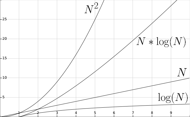
315 Structure Performance Summary
This page will be devoted to summarizing our performance discussions. Below, we have included a graph for a frame of reference for the various functions.
Generic Trees
In the following, $n$ denotes the number of nodes in the tree.
- Insert: 1 if we have the parent but $n$ if we have to find the parent
- Access: 1 if we want to access the root but $n$ otherwise
- Find: $n$
- Delete: $n$ if we have to find the parent
- Memory: $n$
Tries
In the following, $m$ denotes the length of a word and $n$ denotes the number of words in the trie.
- Insert: $m$
- Access: $m$
- Find: $m$
- Delete: $m$
- Memory: $n\times m$
Binary Trees
In the following, $n$ denotes the number of nodes in the tree.
- Insert: $log_2(n)$ when balanced but $n$ otherwise
- Access: $log_2(n)$ when balanced but $n$ otherwise
- Find: $log_2(n)$ when balanced but $n$ otherwise
- Delete: $log_2(n)$ when balanced but $n$ otherwise
- Memory: $n$
Matrix Graph
In the following, $n$ denotes the number of nodes in the graph.
- Insert Node: $n$
- Access Node: 1
- Find Node: $n$
- Delete Node: $n$
- Insert Edge: 1
- Access Edge: 1
- Find Neighbors: $n$
- Delete Edge: 1
- Memory: $n^2$
List Graph
In the following, $n$ denotes the number of nodes in the graph and $e$ denotes the number of edges.
- Insert Node: $n$
- Access Node: 1
- Find Node: $n$
- Delete Node: $n$
- Insert Edge: $n$
- Access Edge: $n$
- Find Neighbors: 1
- Delete Edge: $n$
- Memory: $n+e$
Priority Queue
In the following, $n$ denotes the number of elements in the priority queue.
- Insert: $log_2(n)$
- Access Minimum: 1
- Find: $n$
- Remove Minimum: $log_2(n)$
- Heapify: $n$
- Memory: $n$
Tree Algorithms
We will now discuss the performance of the algorithms that we discussed in this course. When examining the performance of an algorithm we will look at the time and the space that it will require.
- Time: To analyze the time of an algorithm, we will look at the number of operations required to complete the algorithm.
- Space: To analyze the space requirement of an algorithm, we will look at the various variables within the algorithm. To calculate this, we can add up the space requirements for each variable within the algorithm
Preorder and Postorder
function PREORDER(RESULT)
    append ITEM to RESULT
    FOR CHILD in CHILDREN
           CHILD.PREORDER(RESULT)
end function
function POSTORDER(RESULT)
FOR CHILD in CHILDREN
CHILD.POSTORDER(RESULT)
append ITEM to RESULT
end function- Time: The time required for preorder or postorder traversals will be linear with respect to the number of nodes. In a single iteration, we will execute the appending once and we will execute the for loop for each child.
- Space: Since
RESULTis a variable defined and stored outside of the algorithm, it does not factor into our space requirement. Then we must account for the variablesCHILDandCHILDREN. In any given iteration,CHILDwill be constant andCHILDRENwill have size equal to the number of children for the node we are currently at. In total, this would give us a space requirement that is linear with respect to the number of nodes.
Inorder
function INORDER(RESULT)
    LEFTCHILD.INORDER(RESULT)
    append ITEM to RESULT
    RIGHTCHILD.INORDER(RESULT)
end function- Time: For any given call to the inorder traversal, it will execute in constant time. We must factor in that we have a recursive function and as such, we will call the inorder traversal for each node. Thus our time requirement will be linear with respect to the number of nodes.
- Space: Since
RESULTis a variable defined and stored outside of the algorithm, it does not factor into our space requirement. Then we must account for the variableITEM. This will have constant space and thus, the space requirement for the inorder traversal is constant.
Graph Algorithms
Path Searches
1. function DEPTHFIRSTSEARCH(GRAPH,SRC,TAR)
2.     STACK = empty array
3.     DISCOVERED = empty set
4.     PARENT_MAP = empty dictionary
5.     append SRC to STACK
6.     while STACK is not empty
7.         CURR = top of the stack
8.         if CURR not in DISCOVERED
9.             if CURR is TAR
10.                 PATH = empty array
11.                 TRACE = TAR
12.                 while TRACE is not SRC
13.                     append TRACE to PATH
14.                     set TRACE equal to PARENT_MAP[TRACE]
15.                 reverse the order of PATH
16.                 return PATH
17.            add CURR to DISCOVERED
18.            NEIGHS = neighbors of CURR
19.            for EDGE in NEIGHS
20.                NODE = first entry in EDGE
21.                append NODE to STACK
22.                if PARENT_MAP does not have key NODE
23.                    in the PARENT_MAP dictionary set key NODE with value CURR
24. return nothing- Time: The time analysis for the depth first search can be a bit complex. Lines 1 through 5 would execute in near constant time. When we start the while loop on line 6, it is more difficult to analyze how many times this can execute as
STACKcan contain duplicates. In the case that we have a sparse graph, this would be bound by the number of nodes. For a dense graph however, the number of executions would be bound by the number of edges. The code within the while loop would be bound by the number of nodes because of the check that we have not already discovered the node in line 8. If we haven’t discovered it, we would take either the logic of lines 8 through 16 or lines 17 through 23 but never both in the same iteration. Both of these blocks are bound by the number of nodes in our graph. Thus the worst case time requirement would be $n^2$. - Space: Depending on the density of our graph, the space required will be linear with respect to the number of nodes or edges. This is due to the fact that
STACKcan contain duplicate nodes. If we have a sparse graph then it will be bound by the number of nodes. If we have a dense graph then the space is bound by the number of edges.STACK: linear with respect to the number of edgesDISCOVERED: linear with respect to the number of nodesPARENT_MAP: linear with respect to the number of nodesCURR: 1PATH: linear with respect to the number of nodesTRACE: 1NEIGHS: linear with respect to the number of neighborsEDGE: 1NODE: 1
1. function BREADTHFIRSTSEARCH(GRAPH,SRC,TAR)
2.     QUEUE = empty queue
3.     DISCOVERED = empty set
4.     PARENT_MAP = empty dictionary
5.     add SRC to DISCOVERED
6.     add SRC to QUEUE
7.     while QUEUE is not empty
8.         CURR = first element in QUEUE
9.         if CURR is TAR
10.            PATH = empty list
11.            TRACE = TAR
12.            while TRACE is not SRC
13.                    append TRACE to PATH
14.                    set TRACE equal to PARENT_MAP[TRACE]
15.                reverse the order of PATH
16.                return PATH
17.        NEIGHS = neighbors of CURR
18.        for EDGE in NEIGHS
19.            NODE = first entry in EDGE
20.            if NODE is not in DISCOVERED
21.                add NODE to DISCOVERED
22.                if PARENT_MAP does not have key NODE
23.                    in the PARENT_MAP dictionary set key NODE with value CURR
24.                append NODE to QUEUE
25. return nothing- Time: The run time expected for breadth first search is a bit more straight forward as
QUEUEwill never have duplicates. Lines 1 through 6 will all execute in constant time. The while loop will occur $n$ times where $n$ is the number of nodes. Based on the logic, either 9-16 will execute or 17-24 will execute. Both of these are bound by the number of nodes in terms of time. Each iteration of the while loop will take $n$ time and we do the while loop $n$ times; thus the running time will be $n^2$. - Space: The space required for BFS will be linear with respect to the number of nodes. We have 5 variables which have size bound by the number of nodes. If the number of nodes doubles, then we expect the amount of space to roughly double.
QUEUE: linear with respect to the number of nodesDISCOVERED: linear with respect to the number of nodesPARENT_MAP: linear with respect to the number of nodesCURR: 1PATH: linear with respect to the number of nodesTRACE: 1NEIGHS: linear with respect to the number of nodesEDGE: 1NODE: 1
MSTs
1. function KRUSKAL(GRAPH)
2.     MST = GRAPH without the edges attribute(s)
3.     ALLSETS = an empty list which will contain the sets
4.     for NODE in GRAPH NODES
5.         SET = a set with element NODE
6.         add SET to ALLSETS
7.     EDGES = list of GRAPH's edges
8.     SORTEDEDGES = EDGES sorted by edge weight, smallest to largest
9.     for EDGE in SORTEDEDGES
10.        SRC = source node of EDGE
11.        TAR = target node of EDGE
12.        SRCSET = the set from SETS in which SRC is contained
13.        TARSET = the set form SETS in which TAR is contained
14.        if SRCSET not equal TARSET
15.            UNIONSET = SRCSET union TARSET
16.            add UNIONSET to ALLSETS
17.            remove SRCSET from ALLSETS
18.            remove TARSET from ALLSETS
19.            add EDGE to MST as undirected edge
20. return MST-
Time: The time to initialize
MSTwould be linear with respect to the number of nodes. Regardless of the graph implementation, inserting nodes is constant time and we would do it for the number of nodes inGRAPH. Lines 4-6 would take linear time with respect to the number of nodes. Then lines 9-19 would take linear time with respect to the number of edges as it would execute $e$ times and each operation can be done in constant time, except for searching through the sets and performing set operations, which require $log_2(n)$ time. Thus, Kruskal’s algorithm will take time on the order of $e \times log_2(n)$ in the worst case. -
Space:The required space for Kruskal’s algorithm is dependent on the implementation of the MST. A matrix graph would require $n^2$ space and a list graph we would require $n+e$ space.
MST: matrix graph $n^2$ or list graph $n+e$ALLSETS: linear with respect to the number of nodesNODE: 1GRAPH NODES: linear with respect to the number of nodesSET: 1EDGES: linear with respect to the number of edgesSORTEDEDGES: linear with respect to the number of edgesSRC: 1TAR: 1SRCSET: 1TARSET: 1UNIONSET: 1
1. function PRIM(GRAPH, START)
2.     MST = GRAPH without the edges attribute(s)
3.     VISITED = empty set
4.     add START to VISITED
5.     AVAILEDGES = list of edges where START is the source
6.     sort AVAILEDGES
7.     while VISITED is not all of the nodes
8.         SMLEDGE = smallest edge in AVAILEDGES
9.         SRC = source of SMLEDGE
10.        TAR = target of SMLEDGE
11.        if TAR not in VISITED
12.            add SMLEDGE to MST as undirected edge
13.            add TAR to VISITED
14.            add the edges where TAR is the source to AVAILEDGES
15.        remove SMLEDGE from AVAILEDGES
16.        sort AVAILEDGES
17. return MST- Time without Priority Queue: The time to initialize
MSTwould be linear with respect to the number of nodes. Regardless of the graph implementation, inserting nodes is constant time and we would do it for the number of nodes inGRAPH. With a matrix graph, setting upAVAILEDGESwould take linear time with respect to the number of nodes. With a list graph, this would happen in constant time. Then, we need to get the smallest edge from theAVAILEDGESlist, which would be a linear time operation based on the number of edges, and we must do that once for up to each edge in the graph. So, the worst case running time for Prim’s algorithm is $e^2$. (Our implementation is actually a bit slower than this since we sort the list of available edges each time, but that is technically not necessary - our implementation is closer to $e^2 \times log_2(e)$!) - Time with Priority Queue: We do get an improvement when we choose to implement this with a priority queue. For the most part, the performance is the same. Using a priority queue, heapify would optimize the sorting to happen in linear time with respect to the number of elements. In that case, we can reduce the total running time to on the order of $e \times log_2(n)$, which is the same as Kruskal’s algorithm.
- Space: The required space for Prim’s algorithm is also dependent on the implementation of the MST. A matrix graph would require $n^2$ space and a list graph we would require $n+e$ space.
MST: matrix graph $n^2$ or list graph $n+e$VISITED: linear with respect to the number of nodesAVAILEDGES: linear with respect to the number of edgesSMLEDGE: 1SRC: 1TAR: 1
Shortest Path
1. DIJKSTRAS(GRAPH, SRC)
2.    SIZE = size of GRAPH
3.    DISTS = array with length equal to SIZE
4.    PREVIOUS = array with length equal to SIZE
5.    set all of the entries in PREVIOUS to none
6.    set all of the entries in DISTS to infinity

7.    DISTS[SRC] = 0
8.    PQ = min-priority queue

9.    loop IDX starting at 0 up to SIZE
10.        insert (DISTS[IDX],IDX) into PQ

11.    while PQ is not empty
12.        MIN = REMOVE-MIN from PQ
13.        for NODE in neighbors of MIN
14.            WEIGHT = graph weight between MIN and NODE
15.            CALC = DISTS[MIN] + WEIGHT
16.            if CALC < DISTS[NODE]
17.                DISTS[NODE] = CALC
18.                PREVIOUS[NODE] = MIN
19.                PQIDX = index of NODE in PQ
20.                PQ decrease-key (PQIDX, CALC)
21. return DISTS and PREVIOUS- Time: The time required for Dijkstra’s algorithm will be $n^2$ in the worst case. We would expect lines 1 through 8 to take constant time. The for loop on line 9 would be bound by the number of nodes. We would expect the for loop on line 13 to be bound by the number of nodes. This for loop will execute each time
PQis not empty (line 11), which is bound by the number of nodes. Thus, the block of code starting at 11 will take $n^2$ time to run in the worst case. This means that if we double the number of nodes, then the running time will be quadrupled. The worst case for Dijkstra’s algorithm is characterized by being a very dense graph, meaning each node has a lot of neighbors. If the graph is sparse and our priority queue is efficient, we could expect this running time to be more along the lines of $(n + e) \times log_2(n)$, where $e$ is the number of edges. - Space: The required space for Dijkstra’s algorithm will be linear with respect to the number of nodes. We have 4 variables which have linear size with respect to the number of nodes. We say that this is linear because if we were to double the number of nodes, we would roughly double the space requirement.
SIZE: 1DISTS: linear with respect to the number of nodesPREVIOUS: linear with respect to the number of nodesPQ: linear with respect to the number of nodesIDX: 1MIN: 1NODE: 1NEIGHBORS: linear with respect to the number of nodesWEIGHT: 1CALC: 1PQIDX: 1
310 Structure Performance Summary
Stacks
A stack is a data structure with two main operations that are simple in concept. One is the push operation that lets you put data into the data structure and the other is the pop operation that lets you get data out of the structure.
A stack is what we call a Last In First Out (LIFO) data structure. That means that when we pop a piece of data off the stack, we get the last piece of data we put on the stack.
Queues
A queue data structure organizes data in a First In, First Out (FIFO) order: the first piece of data put into the queue is the first piece of data available to remove from the queue.
Lists
A list is a data structure that holds a sequence of data, such as the shopping list shown below. Each list has a head item and a tail item, with all other items placed linearly between the head and the tail.
Sets
A set is a collection of elements that are usually related to each other.
Hash Tables
A hash table is an unordered collection of key-value pairs, where each key is unique.
The following table compares the best- and worst-case processing time for many common data structures and operations, expressed in terms of $N$, the number of elements in the structure.
| Data Structure | Insert Best | Insert Worst | Access Best | Access Worst | Find Best | Find Worst | Delete Best | Delete Worst |
|---|---|---|---|---|---|---|---|---|
| Unsorted Array | $1$ | $1$ | $1$ | $1$ | $N$ | $N$ | $N$ | $N$ |
| Sorted Array | $\text{lg}(N)$ | $N$ | $1$ | $1$ | $\text{lg}(N)$ | $\text{lg}(N)$ | $\text{lg}(N)$ | $N$ |
| Array Stack (LIFO) | $1$ | $1$ | $1$ | $1$ | $N$ | $N$ | $1$ | $1$ |
| Array Queue (FIFO) | $1$ | $1$ | $1$ | $1$ | $N$ | $N$ | $1$ | $1$ |
| Unsorted Linked List | $1$ | $1$ | $N$ | $N$ | $N$ | $N$ | $N$ | $N$ |
| Sorted Linked List | $N$ | $N$ | $N$ | $N$ | $N$ | $N$ | $N$ | $N$ |
| Linked List Stack (LIFO) | $1$ | $1$ | $1$ | $1$ | $N$ | $N$ | $1$ | $1$ |
| Linked List Queue (FIFO) | $1$ | $1$ | $1$ | $1$ | $N$ | $N$ | $1$ | $1$ |
| Hash Table | $1$ | $N$ | $1$ | $N$ | $N$ | $N$ | $1$ | $N$ |
Chapter 60
Requirements Analysis
Welcome!
This page is the main page for Requirements Analysis
Subsections of Requirements Analysis
Module Outline
YouTube VideoIn this module, we will discuss how we can determine which data structure we should choose when storing real-world data. We’ll typically make this decision based on the characteristics of the data we would like to store. In general, the data structures we’ve learned often work together well and complement each other, as we saw in Dijkstra’s algorithm. In some cases, one structure can be utilized to implement another, such as using a linked list to implement a stack or a queue.
When selecting a data structure for a particular data set, there are a few considerations we should keep in mind.
Does it Work?
The first consideration is: does this data structure work for our data? To answer this, we would want to the characteristics in the data and then determine if our chosen data structure:
- maintains relationships between elements?
- translates well to the real world data?
- efficiently stores the data without extra overhead?
- can store all aspects of the data clearly and concisely?
Will Someone Else Understand?
Once we have chosen a possible data structure, we also must consider if the choice clearly makes sense to another person who reviews our work. Some questions we may want to ask:
- is this a natural choice?
- if I look back at this 6 months from now, would I understand it?
- do I need to provide extra comments or documentation to explain this choice?
Does it Perform Well?
Finally, we should always consider the performance of our program when selecting a data structure. In some cases, the most straightforward data structure may not always be the most efficient, so at times there is a trade off between performance and simplicity. Consider the hash table structure - it may seem like a more complicated array or linked list. But, if we need to find a specific item in the structure, a hash table is typically much faster due to the use of hashes. That increase in complexity pays off in faster performance. So, when analyzing data structures for performance, we typically look at these things:
- performance time for tasks
- space requirements
- complexity of the code
We will address this particular facet in the next chapter. For now, we will focus on the first two portions.
Types of Data
YouTube VideoThe first step toward determining which data structure to use relies heavily on the format of the data. By looking at the data and trying to understand what it contains and how it works, we can get a better idea of what data structure would work best to represent the data. Here, we will discuss some main types of data that we could encounter.
Unique
Unique data is the type of data where each element in a group must be unique - there can be no duplicates. However, in many cases the data itself doesn’t have a sequence or fixed ordering, we simply care if an element is present in the group or not. Some examples of unique data:
- car license plates
- personnel ID badge numbers
This data is best stored in the set data structure, usually built using a hash table as we learned previously.
However, many times this data may be included along with other data (a person’s ID number is part of the person’s record), so sets are rarely used in practice. Instead, we can simply modify other data structures to enforce the uniqueness property we desire on those attributes. In addition, we see this concept come up again in relational databases, where particular attributes can be assigned a property to enforce the rule that each element must be unique.
Linear
Linear data refers to data that has a sequence or fixed ordering. This can include
- a series of characters
- a list of steps
- a log of actions taken over time
This data is typically stored in the array or linked list data structure, depending on how we intend to use it and what algorithms will be performed on the data.
We can think of this type of data as precisely one after another. This means that from one element there will be exactly one “next” element.
Finally, we can also adapt these data structures to represent FIFO (first-in, first-out) and LIFO (last-in, first-out) data structures using queues and stacks. As we saw previously, most implementations of queues and stacks are simply adaptations of existing linear data structures, usually the linked list.
Associative
Associative data is data where a key is associated with a value, usually in order to quickly find and retrieve the value based on its key. Some examples are:
- student records associated with a student ID
- tax forms stored with a social security number
We typically use a hash table to store this data in our programs.
However, in many cases this data could also be stored in a relational database just as easily, and in most industry programs that may also be a good choice here. Since we haven’t yet learned about relational databases, we’ll just continue to use hash tables for now.
Hierarchical
Hierarchical data refers to data where elements can be seen as above, below, or on the same level as other elements. This can include
- corporate ladders
- lineage
- file systems
In contrast to linear data, hierarchical data can have multiple elements following a single element. In hierarchical data, each element has exactly one element prior to it. We typically use some form of a tree data structure to store hierarchical data.
Relational
Relational data refers to data where elements are ‘close to’ or ‘far from’ other elements. We can also think of this as ‘more similar’ and ’less similar’ as well. This can include
- cities
- computer components
- social media posts
- graphics
In a relational data set, any element can be ‘related’ to any other element. We typically use a graph data structure to store relational data.
Prioritized
The last type of data we will discuss is prioritized data. Here, we want to store a data element along with a priority, and then be able to quickly retrieve the element with the highest or lowest priority, depending on use. This could include:
- process switching inside of a computer operating system
- delivery tasks to perform
- repairs needed on a device
For this data, we typically use an implementation of a priority queue based on a heap. It is important to remember that the heap does not store the data in sorted order - otherwise we would just use a linear data structure for this. Instead, it guarantees that the next element is always stored at the front of the structure for easy access, and it includes a process to quickly determine the new next element. We’ll learn a bit more about why this is so helpful in the next chapter covering performance.
Info
It is important to note that when we are given a set of requirements for a project, the developer may not use the words to classify the types of data. Based on what a user tells us, we want to be able to infer what kind of shape the data could take.
Trees
In general, trees are good for hierarchical data. While trees can be used for linear data, it is inefficient to implement them in that way (from a certain point of view, a linked list is simply a tree where each node can only have one child). When data points have many predecessors, trees cannot be used. Thus, trees are not suitable for most relational data.
Trees
To recap, we defined a tree as having the following structure:
- There must be a single root,
- Each child node has a single parent node,
- It must be fully connected (no disjoint parts), and
- There can be no cycles (no loops).
In this course, we used trees to represent family lineage and biologic classifications. Once we have the data in a tree, we can perform both preorder and postorder traversals to see all of the data, and we can use the structure of the tree to determine if two elements are related as ancestor and descendant or not.
We added constraints to trees to give us special types of trees, discussed below.
Tries
A trie is a type of tree with some special characteristics, which are:
- Each node contains a single character, with the root node containing an empty character by convention
- By starting at the root and traversing parent to children relationships, we can build user-defined words using those characters, and
- Each node has a boolean property to indicate if it is the end of a word.
Tries are best suited for data sets in which elements have similar prefixes. In this course we focused on tries to represent words in a language, which is the most common use of tries. We used tries for an auto-complete style application.

Tries are a very efficient way of storing dense hierarchical data, since each node in the trie only stores a single portion of the overall data. They also allow quickly looking up if a particular element or path exists - usually much quicker than looking through a linear list of words.
Binary Trees
A binary tree is a type of tree with some special characteristics, which are:
- Each node has at most 2 children (nodes can have 0, 1, or 2 children), and
- unlike general trees, the children in a binary tree are not an unordered set. The children must be ordered such that:
- all of the descendants in the left tree are less than the parent’s value, and
- all of the descendants in the right tree are greater than the parent’s value
Binary trees are the ideal structure to use when we have a data set with a well defined ordering. Once we have the data stored in a binary tree, we can also do an inorder traversal, which will access the elements in the tree in sorted order. We will discuss in the next chapter why we might want to choose a binary tree based on its performance.
Graphs
Graphs are a good data structure for relational data. This would include data in which elements can have some sort of similarity or distance defined between those elements. This measure of similarity between elements can be defined as realistically or abstractly as needed for the data set. The distance can be as simple as listing neighbors or adjacent elements.
Graphs
Graphs are multidimensional data structures that can represent many different types of data using nodes and edges. We can have graphs that are weighted and/or directed and we have introduced two ways we can represent graphs:
Matrix Graphs
The first implementation of graphs that we looked at were matrix graphs. In this implementation, we had an array for the nodes and a two dimensional array for all of the possible edges.
List Graphs
The second implementation of graphs were list graphs. For this implementation, we had a single array of graph node objects where the graph node objects tracked their own edges.
Recall that we discussed sparse and dense graphs. Matrix graphs are better for dense graphs since a majority of the elements in the two dimensional array of edges will be filled. A great example of a dense graph would be relationships in a small community, where each person is connected to each other person in some way.
List graphs are better for sparse graphs, since each node only needs to store the outgoing edges it is connected to. This eliminates a large amount of the overhead that would be present in a matrix graph if there were thousands of nodes and each node was only connected to a few other nodes. A great example of a sparse graph would be a larger social network such as Facebook. Facebook has over a billion users, but each user has on average only a few hundred connections. So, it is much easier to store a list of those few hundred connections instead of a two dimensional matrix that has over one quintillion ($10^{18}$) elements.
In the next chapter, we will discuss the specific implications of using one or the other. However, in our requirement analysis it is important to take this into consideration. If we have relational data where many elements are considered to be connected to many other elements, then a matrix graph will be preferred. If the elements of our data set are infrequently connected, then a list graph is the better choice.
Priority Queues
The last structure we covered were priority queues. On their own, these are good for hierarchical data. We discussed using priority queues for ticketing systems where the priority is the cost or urgency. In the project, we utilized priority queues in conjunction with Dijkstra’s algorithm.
Priority Queues
A priority queue is a data structure which contains elements and each element has an associated priority value. The priority for an element corresponds to its importance. For this course, we implemented priority queues using heaps.
A key point of priority queues is that the priority for a value can change. This is reflected by nodes moving up (via push up) or down (via push down) through the priority queue.
In contrast, a tree has a generally fixed order. Consider the file tree as a conceptual example, it is not practical for a parent folder to switch places with a child folder.
Examples
YouTube VideoIn real world applications, it won’t always be a straightforward choice to use one structure over another. Users may come to us with unclear ideas of what they are looking for and we will need to be able to infer what structure is best suited for their needs based on what we can learn from them. Typically, those describing applications to us may not be familiar with the nomenclature we use as programmers. Instead, we have to look for clues about how the data is structured and used to help us choose the most appropriate data structures
Below we have some examples with possible solutions. We say possible solutions because there may be other ways that we could implement things. It is important that no matter what structure or algorithm we use, we should always document why we chose our answer. If someone else were to join on the project at a later time, it is important that they understand our reasoning.
Costume Shop
A manager at a costume shop has requested that we do some data management for their online catalog. They say:
- Users should be able to refine their search first based on who the costumes are for (adults, children, dogs), then on the part of the costume (tops, bottoms, shoes, props) and then display those options for the user.
- I would like if we could recommend costumes to customers based on their searches.
Take a moment to think on how you might go about this. Remember, there can be multiple ways of solving these problems. We need to be sure that we can articulate and justify our answers.
This is a situation where we could potentially use all three data structures!
First, we could use a tree to represent the search refinement. Thinking along the lines of a data structure, each category and subsequently each product will have exactly one parent. While something like ‘wigs’ shows up in all three categories, you wouldn’t want dog wigs showing up in a search for adult wigs. Thus, there is a unique ancestry for each category and product.

In this scenario we had a fixed ordering of our hierarchy. If the manager wanted users to be able to sort by costume part and then who it was for, our tree would not hold up.
The second portion that was requested was a recommendation system. We could implement this in two parts. The first would be a graph in which the nodes are the products and they are connected based on the similarity of the products.
For example, a purple childrens wig will be very similar to a childrens blue wig but it would be very different from an adults clown shoes. Thus, our graph would have a heavily weighted connection between the childrens purple and blue wig and there would be an edge with a very small weight between the purple wig and adult clown shoes. We can obtain this information from the manager. Since each product will be connected to every other product, a matrix graph would be best suited here.
Then once we have the graph, we could implement a priority queue. The priority queue would be built based off of the users search. When a user searches for a product, we would refer to our graph and get other similar products and enqueue them. The priority would be similarity to the searched products and the item would be the recommended product. As they continue to search, we would dequeue an element if the user selects it and we would change the priority of elements based on commonalities in the searches.
Video Game
A friend approaches you about their idea for a video game and ask how they could use different data structures to produce the game. They tell us about their game which is a sandbox game with no defined goals. Users can do tasks at their own chosen speed and there is no real “completion” of the game. They say:
- I want users to be able to see the tasks that are available to them and what the payout of the task is. It would be really awesome if we could display around 4 tasks that would earn them the most points.
- I have a set of “shortcuts” that users can use to streamline basic functions like switching tools. It would make sense that all of the shortcuts for switching tools start with the same button clicks. So switching to a shovel would be similar to switching to a hammer.
- I have this world in mind that is a lot like our world in terms of terrain and what not. I want players to be able to dig in the dirt and then move that dirt as they like! They could build dirt piles or houses from the trees.
Take a moment to think on how you might go about this. Remember, there can be multiple ways of solving these problems. We need to be sure that we can articulate and justify our answers.
Again, this is a situation where we could potentially use three data structures!
We can use a priority queue to suggest tasks for the players to do. In this priority queue, the priority would be the payout and the item would be the task itself. As tasks get completed, we would dequeue them.
We can use a trie to represent the set of shortcuts. Below is a small sample of how we can implement our trie.

Since our friend mentioned that similar tasks should have similar combinations, a trie will fit well. These key combinations will have similar prefixes, so we can save ourselves space to store them by using a trie.
Finally, for the world layout we could use a graph. Similar to the maze project or weather station project, we can have nodes represent points on a plot and the edges will represent connections. The nodes will now have three coordinates, (x,y,z), rather than two, (x,y) or (latitude, longitude) and they will have an associated type (dirt, tree, rock, etc.).

Two nodes will be connected if they directly adjacent. Players can harvest cubes such as soil or limestone, and it would be removed from the world. We would utilize our remove node function to reflect this kind of action. Similarly, players can build up the world in spaces that allow, such as the dirt pile in an open area, and for that we can use our add node function as well as the appropriate add edge functions.
In our implementation of a graph, it would be better to use a list graph. Each block will be connected to at most six other blocks.
