Single Table Queries Part 1

Video Transcription

Hello everyone, In this video series, we’re going to be taking a look at some simple queries. Now, in this, in this video series, we’ll cover quite a few things, everything you need to know about a full simple query, including how to how to select columns, pick tables out the table that you want to actually pull data from, and filtering those results from those tables. Now, in a lot of programming languages, like Python, for example, everything is an object. And very similar idea here with databases, and particularly with SQL Server, almost every single thing inside of it is considered an object. So each of your tables there, we’ll be talking about views, procedures, and there’s even some functions, and all sorts of other things that we’ll be covering in this course.

But everything is treated as an object. But those objects are contained in what we call a schema. So in if you’re talking about programming languages, like for example, C sharp, your schemas considered your namespace, so everything lives inside of this, you can kind of almost treat this as like a folder, right. And inside, on your computer, you probably have your courses organized or your your information and documents for each of your courses, each of those courses underneath a single folder. And inside of those, you have individual documents and things like that. And so very similar idea of what we have with databases, but instead of calling it a folder, we’re going to refer to that as a schema. Now, a schema itself cannot have other schemas inside of it. So if we’re talking about folders, it’s a folder that can’t have any sub folders. But it is going to contain all of the objects associated with the database. So all of your tables, any stored procedures, and queries that we have saved out, and everything that is associated with it.

So how do we actually refer to the schema, very similar to how we refer to classes and objects in your programming language. So if you’re talking about Python, it’s the package name, dot and then the item or member inside of that particular Python package like a class or a function, and similar idea of what you see in Java. So in this case, we have and will, in the examples that I’ll show here and a little bit, we have a sale schema. And in that sales schema, we have a series of tables that we’re going to work with. So here I am selecting everything, so select star, and we’ll talk about this query here in a minute, but select everything from the sales dot orders table. So sales being the schema and orders being the actual table name. So what do we need to actually have a table. So we, in our early videos, we created a very simple table, we talked about what a table actually contains. So we have attributes which are columns, and then we have rows as well.

So each row representing a actual Single, single record inside of that table. But a table itself is going to have a table must belong to a schema, you can’t have just this orphan table out there, that doesn’t belong to anything. So a table must belong to a schema, which is essentially going to break down to being your database, right? A table must also have at least one column, right? So we can’t have a, we can have a table with no records in it. So no rows, but we cannot have a table that has no columns, because otherwise we have nothing to actually define the data that’s actually being stored there. So as far as the column goes, each column must have a unique name. And that only has to be unique within the actual table itself. So if I have Table A, which has a phone number or email for example, Table A can have email and Table B can also have email. But within each table, we cannot have two columns that are the same name, because otherwise we cannot uniquely identify a particular attribute for any record. So must be unique name. We must also define a data type.

So this is particularly with SQL. Each attribute must have a defined data type. So no change whatsoever. If you’re coming at this from the Java, the Java point of view, but if you’re coming from Python, unfortunately, we do have to actually define the data types here for for each of our columns, and we must also define whether it is null or not null. And the null ability at the null ability modifier here is going to indicate to SQL Server or your database whether or not this column is optional. Hey, so no allows records to be inserted into this table without that column present. So if I have a record, and the phone number is optional, for this particular table, I can insert a record about let’s say, a person. And that person doesn’t have to have a phone number in order to be inserted into this table. Not Null is going to make that column required for all records that exist inside of that table. Now all of this is actually specifically for SQL. We will talk about way later and into the course, I will talk about something called no SQL, which has a little bit more relaxed requirements as far as what the tables are defined, and the types and things like that, which is a little bit more related to what you would expect from kind of like the Pythonic and the Python environments. But these are the minimum requirements that we need in order to actually have a table be a table. So what about a query, right, we’ve talked about and executed a few queries before.

So now we’re really going to kind of dive into what a query is, and kind of define all the individual parts. So SQL itself is a declarative language, meaning that we are going to define what we want not how to get it, which is kind of a backwards thing of what we actually are used to, right. So the the data already that the SQL Server itself, right, the seek the server management system, their job or its job is only to or it SQL Servers job or the or the databases job is going to be responsible for knowing how to retrieve the data, right? The data is stored on the computer somewhere, all your SQL knows as you are connected to, to that particular database, and the database is going to handle retrieving the actual data, all of the SQL is going to actually define or the query is going to define is what you actually want out of that. So what data do you want? Not how do you actually retrieve that data, which is a little bit different compared to how you are working with Python or Java, right? If you are, for example, wanting to read in a text file, and then write out contents to it, you actually have to tell the computer where that file is, you have to actually physically tell you have to tell the language, how to open that file, how to read that file, and then how to write to that file. Which is completely different in most database languages especially. And what we’re working with here is that we are not having to tell the database, how to write it, where and where to actually store it and everything like that. The database itself knows how to actually handle all those operations, which makes our lives as database database engineers to make our lives significantly easier.

SQL itself is a set based language, meaning that for things like C sharp, Java, Python, it’s not procedural or really like any other language that you’ve actually worked with. Really, order itself is not always super important, although we will talk about order on how things work with the actual SQL language, because the SQL statements are consumed in a specific order, but you can actually have them in whatever order you’d like. So very rarely does order actually matter versus a actual program written in Java, C sharp, Python, whatever language really, order absolutely matters, right? It’s top down. Or if you’re looking to a function, it works on line one, line two line three, and so on. But SQL is quite a little bit different than that. And when we’re working with any kind of data and our database, particularly with SQL, everything is going to be dealing with sets, right, a set of data, meaning things are unique. And we have, we can have duplicates in that. But we’ll be diving into a little bit more about what that set is going to kind of mean here in here in a moment. So common problems. So as we get started with working with SQL and SQL Server, there are some common pitfalls that some students or or, or people who are new to writing SQL fall into.

So one is that you disregard one of these properties, right? The fact that sequel is set oriented, and declarative, so we are trying to reverse you’re, you’re not completely reversed on us as far as how we’re actually writing SQL code. But it’s not line by line by line, right. And this becomes significantly more important, as we add more and more to our queries, as our queries get more and more complex. If you’re thinking about it in a as a procedural language, from you know, top down, then it’s not necessarily going to work out, the logic won’t actually end up executing as you expect it to, and you’ll end up with a lot of different results or results that you don’t expect. So Okay. Oops, sorry, one second to those who are recording. Okay, so, in this class will be I will be referring to or you’ll see these acronyms, quite often. DDL and DML. Okay. So DML, which is what we’ll be working with, for the majority of this course, is referred as stands for data manipulation language. Okay. So with DML, this is all of the query statements that you’re going to use to retrieve data or modified data. So inserting data into your tables, updating data, or updating records that already exist, deleting them, merging them, and just flat out retrieving them like select. On the other hand, we also have data definition language, or DDL. And this deals with primarily creating data. And not just necessarily creating data, but creating databases and creating tables, views and stored procedures and things like that also fall into this category. But we won’t get to those particular parts until later in the course. This first section of the course will be focusing primarily on just the SQL for database manipulation, or data manipulation.

SELECT FROM

Video Transcription

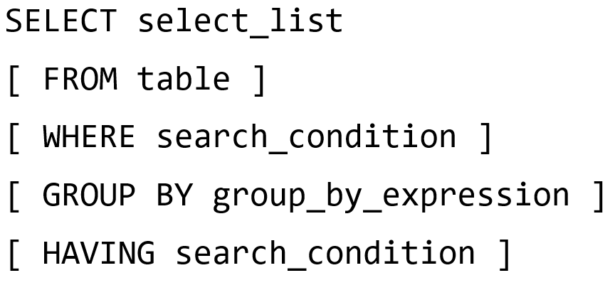
Alright, so now that we have reviewed some of the basics, let’s go back to writing some actual queries. So we’ve already ran some basic select queries before, but we didn’t really break them down into into what each part actually contains. So we’ll start out first by looking at a select, but without the from clause. So the from clause is actually optional. But the Select is required. So this is the SQL syntax here. And I will show more things like this as we add more statements and elements to our SQL query. But this is about as basic as you can go. And then the square brackets there, that denotes an optional element. So the from clause is optional. But let’s without further ado, take a look at select select is the only thing required in a SELECT clause. So we don’t actually have to have a table to pull from, we can actually project data just without any initial data source, though usually, and the vast majority of queries you’ll actually use, we will have a From clause associated with the select. So you select these columns from this table, or from this data source, essentially was what that boils out to, can also rename the columns that we actually select. If our database design is done correctly, or done well, so to speak, we shouldn’t have to add a lot of aliasing here. But column alias aliases are really helpful when we are pulling data from multiple tables. And then also when we’re actually showcasing query results back to the actual user. Because a lot of times the database column names aren’t necessarily super user friendly. As far as in the user, it may be fine for a database engineer designer, but not so much for the end end result. I’ll showcase some aliasing here in just a second.

But the SELECT clause is going to be the projection operation within aren’t you know, if we want to use database terms here, now are sorry, sets. So with sets, we have projection and selection, and for some reason, when the SQL language was being designed, they chose the select keyword to set to for the projection operation, and the from clause to be part of the selection operation. And so it’s it’s kind of backwards as far as the actual SQL statements go. What it really boils down to for the Select or projection operation is that we are picking out which columns or attributes of our data that we actually want to have come out and the end results. So if we have five columns in a table or a set, we are going to project or select a, either all of those columns or a subset of those columns. So maybe column one, two, and five, and we’ll skip the other two. That’s what projection is going to do. And here in a few here in a moment, as well, I’ll show you the from clause, which is the selection operation, which deals with rows instead of columns. Without further ado, let’s take a look at a couple of examples of our select. Now, as I was mentioning earlier, we do not have to have an actual table to select from. So I can go in here and say select seven and run it and I actually get a result. So I end up with one row one column. I don’t have a column name yet. But there it is. There’s my data that from my for my query result.

Now a lot of times you won’t actually see queries as simple, but sometimes they’re actually pretty useful. But nonetheless, I can actually go back in here and this is where aliasing becomes very useful. And so we will say as, and then we can, let’s say number here. Cool. Now, as I run that now, I actually get a readable column name out, so I get a number. There. Also notice here, when I look at number, you’ll notice that it is is highlighted in blue. So things that are kind of reserved words just kind of like as you’re typing and your favorite programming environment, it highlights key words as part of the language. So if you have that situation here, or you end up wanting to have a space and your column name, then you will need to do something like this. So we want to actually denote the actual name either using square brackets, which is going to be the way that SQL Server usually will prefer it, you’ll see that and other database languages or other SQL flavors, you will see this as a double quotes. So either one works. For me, I do not mind either way, which way you go. Most of my examples, you will see me using the square brackets, just because it’s more SQL Server II ish. But the double quotes are also perfectly acceptable and perfectly acceptable syntax.

Now we can do all sorts of things here as well, like I can add more columns, so I can do. Right, and I actually get a text column back out, I can even put a date. So state time offset, this function will actually pull out the current time on my local computer or the SQL Server instance, the time from that server server. Now see, if I do a space here, it doesn’t really work out so well. But if I actually wrap that in either quotes, or the square bracket to denote the actual name, I can actually have a space now on my column name, this is really as simple as a, an expression as you can get as far as being a complete and full query. Okay. Now, a couple other random thoughts here, the capitalization of the actual SELECT statement or or clause elements, doesn’t really matter, right, it is not case sensitive as far as select. So I could go in here and do all all lowercase if I want it to, so I could go select. And that will still execute. It is common syntax for people to use all caps for any SQL elements, and queries, because that helps denote it from the rest of the content. So it helps to note away from column names, values, conditions, all sorts of other things that are not reserved words in a SQL query. So that is the primary reason why we use all caps for any SQL statements. That just helps us pick out the keywords a little bit easier, especially if we don’t have an IDE that is doing all of the coloring for us.

Okay, so let’s keep on moving forward here on to the from clause. So from is going to actually denote what table or tables your query is actually pulling data from. So in other words, it tells the query where all the data is coming from, you’re going to use from a lot of different contexts. And tables can be defined relatively loosely. For for now, our simple queries are going to pull from one single table inside of our, our schema or schema database. But there is a lot more that can kind of fall underneath the from clause. As we’ll see later in the class. We can use aliases as well for the from clause. So we can say from table XYZ as x, you know, whatever name we actually want to put for the table. So the aliases work the same way as a SELECT clause. And the names though that are available to the select clause, are are extracted from or inherited from the result of the from clause. So that’s how select happens right? So we actually even though we list select first in the SQL, the from clause actually has to execute first because the Select has to know what columns are available to it to actually purchase So we’ll take the the columns from the from clause, so all the columns from the table or tables that are in the from clause get passed to the select clause.

For projecting, let’s take a look at an example of this and action here. So we had this piece of SQL way earlier in these video series, so select star from sales orders. And you can notice here I get 1000s of rows in this sales orders table is from the worldwide importers database. If you don’t quite have that selected, please see the the setup video that’s out there, or feel free to reach out. And I can help you get that worldwide importers database set up for you. Because sometimes it can be a little bit tricky. But this database was provided by Microsoft, as an example database. So we’ll be using a lot of this database a lot in the lecture notes. So but as you can see here, lots of different sales information, we’ve got orders, we’ve got customer, the customer that made that order, who sold to that customer, and then all sorts of other things here as well order date and a variety of other things. So if I go down here, there’s actually quite a lot of columns in this table. So select star can be kind of kind of annoying, as far as as far as that goes, he very rarely need all of the columns from a given table. So as far as efficiency goes, it is far more efficient to select the specific table or the the specific columns from the specific table that you’re looking for.

Right. So for example, I maybe I only want something, say orders, maybe I only want the order ID and then the date that that order was made. And then the customer that made it, do customer ID. Now if I run this again, aha, my my results are far more clean, right, there’s a lot less information there that I need to actually consume. So column names default to whatever the tables column names actually are in the database. If it’s a direct reference, you can actually put the column name without the table that’s associated with it. That is perfectly fine, perfectly valid syntax. However, when you start to do multi table queries, it becomes less clear which column comes from which table. So it is more more common and better practice to always specify the table that that particular that particular column or attribute actually came from. So or dot. And there we go. We can also do the same thing here, right if with an alias, so if I did, as, and then if I really wanted to be shorthand, I can say, oh, but notice now that my syntax no longer works. Because the Orders table does not is not does not exist. It does exist in the database. But it does not exist as far as an option or an available source of information. Because it’s no longer included in my FROM clause. The table that’s included included in my FROM clause, as far as the Select knows, is just Oh. So let’s change that to oh, oh, and we’ll also there we go.

So now, I run that we’re back in business. So things become a little bit easier to actually do there with aliases, especially if you have like, a really long, like long schema name or a long table name. Sometimes the aliases are really nice. Just add a little shortcut there. And that’s relatively common practice. And as long as you don’t have a ton of tables, single character aliases are fine. But if you have a really big complicated query, this is you use good practice and naming your variables in your code. You want to use good practice in naming things like aliases inside of your SQL for our order date here, we can actually change this up a little bit. We can repeat, we can project a column more than once. And what do I mean by that? Well, what if I add here? The order year? Right. So there is this handy dandy function called year. And again, we’ll use I’ll show more more functionality with the date time format stuff here later, but I can say year here, and if I run that, I get the order year so just the year out of the date that’s full date is still there. Although I should probably add a alias here. Just to be a little bit easier to easier to run. That is just the basic select from here and the next series of videos. The next video, we’ll look at expanding our simple query

WHERE

Video Transcription

So now that we have actually worked a little bit with select and from So specifying which tables we want to pull data from, and which columns from those from those tables we want. Now we can actually filter which rows that we want. So the from clause is again, right the selection operation, right. So it is all of the rows, all of the rows of data that we want to pull as part of our query. Now, select does filter a little bit, but it filters only vertically. So it filters which columns actually end up showing up. But to filter which rows show up, we need the where clause, the where clause, as I mentioned, just provides the basic filtering per row. And now it will accept any predicate or Boolean expression as part of it. So all of the Boolean expressions that you’ve learned so far in just your basic programming, will actually apply here, for the most part. So we are partially supporting the selection operations.

So from gives me all of the rows from a particular table or tables. And if I ever want, if I want to reduce the number of rows in that set, I use the where clause. So I’m filtering out which rows actually end up showing. So let’s take a look at a few examples here, a little bit easier to actually see this in action, rather than listening here to me talk about them. So let’s add a new cell down here. So as we saw before, from our, our larger query, so if I run that again, right, we have large 1000s and 1000s of rows there. So how do we actually reduce that to be only a specific set. So if we take this same exact query that we had, right, and then I’m going to add to this a where clause. So select from where, and then I’m going to say year, O dot, order date, and then set that is that equal to 2016, since we are only doing orders of 2016. So now, if you run that and look at the order date, so nice, my the number of rows that actually have here are significantly fewer. And my order date is only 2016. orders that have a year of 2016. So the Boolean operations are very similar to what you would expect in Python or Java. Of course, now I’m not using the double equals for equality, I’m using the single equals which can be confusing. In this context, when used in the where clause, it is not an assignment operator, it is the equality operator for the UI for a Boolean expression.

Now, years are kind of tricky. What I have here is a specific order date, but I actually have to convert the way I’m actually writing this code, I’m converting each time each date, so year, month, day, to a single year. So I take the full year, convert it into a car full date, and then convert it to just a year. But I can do this exact same thing down here by just doing a range on the date instead of having to convert it. And typically that is going to be the preferred way of doing so because it is a little bit more efficient. And with databases, unlike our our code. We want our code to be efficient. But it is more important for SQL queries to be efficient as possible. Because we’re dealing with 1000s upon 1000s of records, the majority of time, think about, you know, writing queries for something like Amazon, right has millions upon millions of things of records there. And so if we have an inefficiency in one of our queries, that adds up to a significant amount of extra processing time over some period on our servers, and of course, a worse experience for the our our end user. So we do want to be as efficient as we possibly can. So let’s go in here and say order date. And then we are going to do, we’re going to use like a greater than or equal to here. So and I’m going to put the date here as a stream. And so this is an easy way to do this, this doesn’t have to be an official date time datatype as long as the string matches what we’re actually looking at, so we’re doing one one of 2016, so January 1 2016. And then we are going to put an AND operator here, so and ODOT, order date, order date, and you’ll find the IntelliSense with SQL is hit and miss that time.

So whether you’re in your Azure Data Studio, or SQL Management Studio, or whatever your IDE you’re using IntelliSense can be hit and miss, which is what’s happening there. But anyway, so let’s, let’s put, we want our, our date to be less than 2017. So we’ll put the first of January of 2017. Now I could I could put the end of 2016. And do make sure make this less than or equal to, that also would have worked. And then we’ll close that off with our clause. See here, that’s where my mistake was I had an extra semicolon, semicolon, by the way, as I’m showing you here, denotes the end of a SQL statement. Okay, run that. And there we go, I get all again, all of the orders that were made in 2016. But this is actually a little bit more efficient than the query that I showed previously, where I’m converting the date to a year and then comparing it to the number here, I just compare the date directly without actually modifying its format. And I’ll be showing a variety of these little things as we’re working through our examples here and through assignments. The code I’m the sequel that I’m using here is a very basic WHERE clause write this using a date, but your where clause is essentially used on any column, that that is being available or projected from our slot, right. So whatever columns are available, I can actually pull them out there. So I’ll actually show some of the orders or some of the sets there, but it’s not specific just to the select clause right? The from operates first, then the where and then the select.

So the rows are filtered before they make it to the select. So the selection operation happens with the from and where clause is done before projection. So selection first, then projection. So select actually happens after the from and where clause SQL statements. But here I just used simple equality check. And greater than less than, but there are a lot of different Boolean operators that we can utilize inside of our WHERE clause, and a variety of other places in our SQL statements. booleans though are the only are only supported as expressions. So there is no actual boolean data type. So you know, in Java, we have Boolean. And even in Python, we have a false and true type associated with the language, but SQL really doesn’t. They just use it as expressions. And that’s the vast majority of database management systems. So SQL Server, MySQL, and a variety of others will have very similar similar goes. So where can we use these Boolean expressions. So we’ve already seen them being used in WHERE clause in my examples. But we also have if statements and loops inside of inside of our SQL statements, and we can also have like case a case function, which will I’ll showcase here in a later video.

So the case function is very similar to the switch statement in Java. Although of course, Python does not have a switch statement, but more or less just a shorthand series of ifs. But we’ll get to that here. And not too long, but all the operators that are are all the primary operators that are supported for Boolean are mostly standard except as I mentioned, as you see here, and in my previous example, the equality operator is not enough. equals, it’s just the single equals, we have greater than less than or equal to naught is done a little bit different. So the standard way of doing not is less than greater than. But there are others that are supported like the exclamation points. Okay. So not equal to, not less than not greater than those are supported. But they are not part of the SQL standard. So your mileage may vary, depending on which database language, you’re actually using all SQL, but each, each company implements it in a slightly different flavor.

Most of your languages that we work with write a boolean value, all right, even if we talk about just general logic is true or false, right? There’s no in between. But with databases, we actually introduce a third value called unknown. Unknown, that’s kind of a weird situation, right? Because what happens, if a value is no, most languages know is going to come back as false or false see, because no being the absence of value, the absence of value cannot be true, because there’s nothing there, which is a lot of the same case in a lot of languages. But with SQL, as you’ll see here, we are going to pull a query like this one sec, let’s clear. Clear that there and run this. So again, write slug star, I’m using Select star, just as a quick example. Try not to get into the habit of using Select star for solutions to things, it is very useful tool to just kind of explore results. But at the end of the day, you’ll want to reduce that and actually specify your columns. But if I run this here, you’ll see that nothing gets returned. Right? Nothing gets returned. Because nothing is no All right, the order date does not actually know. But at the end of the day, right? A lot of the times here, this is going to be still evaluate to true or true, false or on known. Right? So even if it is unknown, right? It’s not going to actually show up.

So if I showcase this here, with this query here, the where clause is filtering the rows by order date, order dates that are not No, right, that are not equal to no. And running these, I still get zero rows, right? Because date, order date is actually a non nullable column. So the order date must exist. But a better way of actually showing this, because there’s also there’s seven like 73,000, some odd 100 rows and the orders. Table. But let’s switch this to a a column. That is no. Okay. So if I flip this back, right. Not no. Oh, dot internal comments, not No, I get nothing as a result. But if I flip this, right, say equal NULL, also, I the results are nothing right, and nothing is actually coming out. But if I flip this to say, is no. I actually get quite a lot of records out. So if I scroll over here, and ternal comments, right? So here you can see internal comments. All of these are actually not no sales orders that have no internal comments. But you notice that the equal sign and the not equals operator, both of those don’t actually work for naught because the Boolean comparison here, all right, a value so no, not equal, no is actually unknown, because we have unknown there so it’s not actually true. So don’t add so those items never actually get returned as a result in your query. So if you are ever working with no or a which is usually the case for for things that are non null or nullable columns. And if you’re trying to check for null, the is operator is usually the preferred way to do the Boolean comparison.

So, this will return true if the internal column comm internal comment is no right. So, if we backtrack this, I can say is I can also say is not no. Right? This is more more so related to Python than it is and how things are compared to Java, right? So we say is, is no, or is none in Python. And instead, and we also have an actual better pit person here. So, we actually have, we can actually showcase this one here, since this is columns are here. So we have a whole bunch of normal columns and we can show those that are not no there. So, these orders have already been picked, the items have already been picked up. So, that’s just another example of how we can utilize Really N expressions. Like said Boolean expressions most commonly are going to be found in your where clause, but as we saw back here on our slide, we can find them in our where clauses, control statements like ifs and loops, as well as our as a case function. You may also see them in a variety of other ways in stored procedures as well. But that will conclude this part. In the next section, we will talk about grouping or group by

GROUP BY - HAVING

Video Transcription

Welcome back everyone. Now in this video we are going to be taking a look at group by and having. So before we took a look at simple SELECT FROM clause or from query, along with where so remember, we select columns from our table, and where is there to filter out the rows. So remember that we have the selection and projection operation. So the selection being the from and where clause. So the selection of what rows of data are we going to include in our results, and then the the projection or the select statement in our SQL query is which columns are we going to include in our on our query result. But now we can actually also group those rows together, right. So after we have whichever rows that we actually have in which columns that we have, we can actually group the results by certain conditions. So each of these though, by the way, right, these are all still all optional items. So if you ever look at the actual official documentation, everything in these square brackets here are optional statements that can be included in your SQL query.

But let’s take a look at group by and having it’s a lot easier to start picking this up, as we start to show some more examples. But groupbuy specifically, is going to define a group based off of a set of call or a set of columns or expressions, right. So based off of whatever the expression is, whether it be some comparison, or a specific column, or two or more, this is what we’re going to group our rows by. So it’s defining the defining the rules that we’re actually doing the grouping by. So this does allow aggregation. So if we, let’s say, group by order date, right, we can get the number of orders for a particular date, right, which is a very useful query to run. And there’s a lot of other different aggregations that we can show here in just a second. There are many options available to the group by element. So we can do a list of columns that we group by, we can group by sets, expressions, and there’s also we call queue roll up, those we’re not really going to cover in this class. But if you’re interested, I am more than happy to tack on a video or post some text up, that kind of explains them. But these are some of the standard operations that you’ll see associated with group by. But most of the time, we’re going to be working with aggregates, so max, min, average, and count.

So those are most of the common aggregates that will actually work with. Now aggregates themselves are almost always this particular syntax. So the function, so the aggregate function that we have on on on the right side there, and so let’s say count, and then in parentheses, you will have an some sort of expression that will tell you or tell the function what to count, right? Out of those rows. So all is the default. And then we can do, we can do distinct, so do we want to count duplicates, for example, right? Or no duplicates. duplicates are no duplicates, and then whatever the expression is, so and I’ll show an example of this here in a few minutes. And as I mentioned before, some examples of this are min max, average, sum and count. Although count is similar, but count allows for no expression. So for some, for example, you can’t sum star right? But count is kind of unique there where we can actually put star as a wildcard and say just count all the things right count all the rows, but for like some min max average, you want to know what specific thing that you are summing up or averaging or finding the maximum right you want to know the specific column out of the group that you’re actually going to apply that function to count is a little bit different count that aggregate function actually returns the number of records or rows that are in that group. But this can be utilized and with the over clause, when we are utilizing partitions. But I’m going to kind of skip over partitions for now. And we will save that topic for another time. But just kind of be aware that it is there in case you see this as you’re looking at this, or reading about this online, but we will talk about partitions in a later lecture.

In this case, no values are ignored by default. So if there is no value of is not included as part of the aggregate, let’s take a look at some examples of the group by Alright, so now I got got myself put up towards the top of the screen. And this simple query, here I am selecting all the customer IDs from the orders and grouping them by the customer ID. So when I group by the customer ID, I am essentially grouping all of the records that are associated for that specific customer. And so if I run this, you actually can end up figuring out how many customers we actually have, or how many unique customers that we actually have here. So this is all of our customers that have placed an order with us. And of course, I can try to add columns here. But this becomes a little bit tricky. So let’s do au dot order date here, I run that I get an error. So this is one of the weird things are not to say or weird things, but not initially intuitive things about the group by clause. So I cannot project an element or an attribute or column. When we have a group buy, and if that column is not inside that group, so I cannot project a column that is not part of the grouping. Because I’m grouping by a specific condition, write an expression right here, I’m grouping by just the customer ID. And so each record, I mean, let me take this off real quick. When I get my query results here, the rows that are fed to the select clause are what you see here on the screen. And so when we have like 1234, for the customer ID, there is no date associated with each of those customer IDs in this case, because those columns have been filtered out already by the group by now I could put the date back in here. Okay, now, let me do this way.

So you can add columns here. Like if I wanted to do an O dot Sales Person ID, and put this up here. And rerun this here. This actually works, because I have the me actually sources here, right. So this will group all of for so for the salesperson, it’ll group them together and all of the actual customer. So if, if customer 531 had 10 orders with this particular salesperson, all of those records will show as one row. But what about the date? Well, the date comes across a little bit easier when we actually do aggregate functions. So if, for example, I take off the salesperson here and put back the ODOT order date, and then instead tack on a let’s say aggregate function now, what happens here? Uh huh There we go. So let’s put that as first order here. But so what I’m doing here is I’m grouping by our customer ID, and then I am going up here in my selection and say, Hey, give me the smallest order date for this customer ID. So, for this group, give me the smallest order out of that group. So for each of the customers I get the date of their first order in this particular table. When I have a group by I cannot project a column if it is not part of the grouped by, but I can project a column if it is part of the group by or I can project it if it is an aggregate, if it is an aggregate, so min max, average sum count all of those sorts of things. So I could here, I can say count, and then star. And this will tell me how many? No orders? So how many orders? Has that customer actually made? So, for each customer, when was their first order? And how many orders did they actually make, right? That is what I’m actually associating here.

So, this is group by group by itself is a very powerful expression. And it really does help combine and aggregate database results in that’ll be a really common operation that you’ll see as we start moving through the class. But let’s talk about how we could actually filter those results. So I showed how you can group your results. So group those rows. And then what about filtering those because the where clause doesn’t actually filter the groups the where clause filters the individual rows, before we get to the group by so the having clause or having element is what we can use to actually filter records after they’ve been grouped. So basically, just like the where clause accepts any Boolean expression that you express, but aggregates, aggregates can actually be used here, right? The WHERE clause cannot use the aggregates because where the where clause is a single row by row operation, the having clause is a group operation. So you have a group of things that you can apply this filter to. So therefore, you can also use aggregates as part of the filtering process. So let’s take a look at an example here, I’m going to replace the query that I had before. Do or here, and sorry, for my bad syntax here, let’s fill this in with count. Okay, so I’m going to run this and we can see what happens.

And I’ll kind of work on explaining this here. So we have our counts here. So this is the number of orders again, as I say, order count. So we have order counts. And then we have our men date here. And I’m actually going to add these to a new line. So they’re a little bit easier to read. And so we have as a first date. And then let’s have that as order year, that’ll work. This is last date. And this is first There we go. Okay, so now I got names on all my columns here. We’ve got order count, first date, last date, order year. So what I am actually grouping by here is the actual order year. And again, I am using a shorter syntax here, converting the order into just the year and grouping by that. But again, though, you can, you can group by the actual raw dates. But here we can actually, we can’t group by a range of dates here, because we can’t do group give me a group that goes from one 120 16 to 1231 2016. Because there’s a lot of dates in between that range. And so you have to give one value that is represented representative of that particular group, we can group by more than one column, by the way, as I showed earlier, but here, we’re just grouping by year.

So for each year, when was the first order? When was the last order and then what was that particular year. And that was our group by, but lots of things that we can actually do with this right? The, with the group by alright, we can actually have, we can actually filter now out specific groups, right, so we can actually filter out specific groups. So let’s take off the semicolon here, and actually add in our having clause now. So select from where group by so from orders where the picking completed when is not no so it’s actually If the order has been completed, fulfilled, group those by year. And for each of those for each of those groups that we have, I am going to specify that I only want the years where we were very successful. Okay. So I want the years are that we successfully completed, let’s say 20,000 orders. And if we look at our results there, that should give us two rows.

So if we run this, oh, yeah, there we go are two rows. So this particular this particular filter, we would not be able to successfully do in the in the where clause, because the where clause is row by row, where the having is group by group. So in having clause we can actually apply a aggregate function to filter out groups that only have certain things there. So that’s a very useful feature there. But that pretty much concludes for the series, the example SQL queries that I’m going to show here in the following video, I’m actually gonna take a quick a short amount of time here to actually talk about the processing order. So as I’ve been talking, I’ve been jumping around in these actual SQL queries, talking about what each part actually does, but there’s actually a very specific order that these actually get executed in so we’ll take a look at that next

Processing Order

Video Transcription

Welcome back, everyone. So this will be our last little video for our single table queries part one series. But in this video, we’ll talk about processing order of our query. Now, before I talked a little bit about how our SQL language is not a procedural language, so we’re not going step by step, line by line from line one to line x, in order that they actually happen. So there’s a different processing order that actually happens than what’s actually shown on the screen. So we talked a lot about the major elements of select, and we’ll talk more about the SELECT query. Later in this class, we’ll add some more elements to it. But the core bits here are SELECT FROM WHERE group by and having are the ones that we’ve talked about so far. Now, the order is not the order that they are shown here on the screen, it does not go from SELECT FROM WHERE group by having, we actually go to the from clause first.

So we need to know the source of our data before we can do before we can do anything, right. And we know nothing until we know where the source is from. Now, I can do the slug claws before without any of the things underneath it, right. So if we just have select by itself, of course, the slug will actually be will be done first. But if we if we have select and other things, select is not the first thing, right? So from this data source, so from XYZ table, where, right, so we filter out the rows from that table, right? So from Table A, we want only the rows that match this particular condition. And then we can then group those rows together by a certain condition, right. So group by color, right? Having, let’s say a count of 10, right. And then we actually select right, we actually do the actual projection. So remember, all of all of this here from where group by and having are all part of the selection operation. And then the select is the projection, right? Select is the which columns are vertically, which things are we actually going to show the forum were grouped by having are all horizontal, so which rows are we going to show, so we pick the rows that we want first, and then we pick the columns from those rows that we want.

But this is really going to be something that I will really work on and repeat quite often in these videos is the processing order because it is not intuitive. When you first start reading SQL, that it is not the order that you read it in that it operates in, it’s a different processing order, it executes in a different order than what is actually shown there on the screen. And just as a review, here, this is just a friendly slide help remind you of all of the different syntax that we actually covered here for our simple single table query. So we have the SELECT clause, and then from were grouped by having this is the typical typical ordering that you’ll actually see them written in and of course that’ll be talked about just before that actually operates executes from where group by having and then select. Now, any one of these down here are optional, right I can have a From clause and not a where clause, but a group by I can have a group by without having, I cannot have a having clause without group by though, having the having clause must be paired with the grouping, because the having is an aggregate filter, not a row by row filter. That is one limitation of the syntax there. But that really concludes the first part of our simple table queries. This is the first part of a three part series that we’ll be talking about, for doing single table queries. I will see you in the next video.

Single Table Queries Part 2

Video Transcription

Welcome back everyone. In this video series, we’re going to continue our talk on single table queries. Now last time, we covered a lot about the SELECT clause, which can be paired with from to choose which tables you’re picking from, and the where clause, which can filter which rows are being picked. And then we also did a little bit with group by and the having clause which filters those groups. So we’ll review those a little bit today. And then we will cover order by distinct Top Offset fetch, and also the process or the order in which those are logically processed inside SQL. So let’s first start out with the having clause, this is what we ended up on in the previous video. So remember, the having clause is a post group filter, right? So meaning the having clause can be used with in place of the where clause which filters row by row. So we have SELECT FROM WHERE, so the from clause picks which tables, so the data source, and then the where clause will filter out any rows that you don’t want. And but where clauses only row by row, likewise, so having is grouped by group, so having an were cannot be used interchangeably. So having can’t be used to filter out rows, or individual rows, and the where clause can’t be used to filter out groups. So that’s why they are separate there.

So the big benefit there that we can have with having versus the where clause is that we can now actually use aggregates, so things like count, average sum, and all those sorts of things can’t be used inside of the where clause, because it is again, right single rows at a time, where the having clause has groups at a time that it can actually filter. And so we can actually use aggregates like counts, like we, like we did last time to filter out groups that don’t meet minimum specifications. And I’ll show another example of that here in just a moment. But I also wanted to introduce again, a nother clause that we didn’t get to last time is the order by now order by does allow us to as it sounds, order our results, which helps out quite a lot in providing some consistency. So by default, your queries aren’t necessarily sorted in any particular order. So for the most part, the results that you retrieve from your database are going to be retrieved in the order that those results were actually entered into your database. But not necessarily always the case, because sometimes that order can get flip flopped or shuffled. So if you are ever concerned about needing a specific order, the order by element or clause is going to be something that is a must to enable that consistency.

So the ORDER BY clause can do ascending and descending orders. So those are the two supported sorts, the ASC or D, S, C are the key words there can follow the expression. So order by ascending order by descending are the keywords that you’re looking there. But ASC or the ascending keyword is the default, the default order, so you can just do order by column without actually specifying which order you want. And by default, it’ll go ascending. So typically, if you ever want to sort anything other than that, you will need to use this, this ending, but the ascending keyword is not required. But nonetheless, let’s take a look at a couple of examples. So I did want to review slightly here, lists is one of the queries that we started to cover last time. So we have order year order count, first order date, and last order dates for all groups of orders by year. So we again remember the from clause is executed first, then the group by in this case and then the SELECT clause, which is again, right not the typical processing order compared to your programming languages.

But here, we’re just grouping all orders by year, which enables us to count the number of total orders for each year. And then we can also pick the min and max date there. But again, remember that we cannot have any columns in the SELECT clause that are not in the group by if we do have columns in the SELECT clause that are are not in the group by, then those must be presented as aggregates as we have here, with the count min, and Max, which are all aggregates, even though the order date, in its raw form are not as not part of the group by or even the star here, things are this is not included in the group by but I can actually do this aggregates per group and project those in the SELECT clause. Again, remember here with those, we have projection, this the set operation projection which is handled by the select that is which column so which vertical selection, the vertical parts of my set, and then the from and group by are going to deal with more of the selection operation, specifying which rows we’re going to have in our result. We also talked about the having clause last time, again, just as a quick review, remember, the having clause is going to filter your groups, right, the having cannot filter out row by row, but it can filter out group by group. And so the benefit there is that we can actually use aggregates here as a result, so we can execute this. There we go. So, now, we only have the order the order years that have more than 20,000 orders in that particular year.

So pretty useful operations here that we can actually start to do some more interesting things with the data that’s stored in our database. Let’s take a look at the order by now as well. So order by is new, we did not have that last time. So order by is going to come after your FROM clause, it will, you can also order but you can also order your groups by the way as well. So if you want to order your groups, the order by is going to come after group by and having clauses. But let’s for sake of simplicity, let’s take the grouping out and try to run this. So here, if I order by my order ID, you can see that I have 1234567, so on and so forth. Now I can show you what that looks like without it. And you can also see here, right that my order ID actually kind of ends up coming out the same. So I didn’t really change much there. This kind of highlights the differences here. But my order here is not guaranteed. Like for example, assuming that, you know my orders are entered in canonical ordering. So order one is first and order, you know XYZ is next. But if I actually end up going back, and let’s say deleting a couple or modifying a couple, let’s say this wasn’t supposed to be order for this is order 20. Well, the ordering then is still is now not guaranteed. So even though in this situation here, my order doesn’t actually change in my results. Adding the ORDER BY clause will actually guarantee the ordering of my results rather than betting on chance.

Now we can actually take out the A S C here, and it gives me the same ordering as I mentioned just a little bit ago. ASC is the default ordering. But we can actually we can order in descending order as well. So we can get the last first instead of the opposite way. We can also let’s say we want to also order by multiple things. So let’s switch this to order date. And let’s order in ascending order there. And then I want to do O dot two customer ID and run that. So this becomes a little bit more powerful right I think can order multiple columns, and I can actually switch this up as well. I can order in descending order and one and ascending order and the other. So it does not matter how, which one is which, necessarily, so you can order ascending or descending on multiple columns. Let’s go back real quick and talk about the processing order here. For these as well, we have seen most of the major parts of our select class, right, so the most common things that you’ll actually see a SELECT query, we’ve seen most of them now. So the standard processing order is not again, it’s not top to bottom, even though we’ll write our queries top to bottom, so select from where group by having order by, we are not going to the sequel is not going to actually be processed in that exact same order.

So from clause is first. So we pick our data source, the tables that we’re pulling from, then we can filter the rows out of those tables. So we can do a first pass of filtering, again, the where clauses single row by row, then we can group those rows together based off of some expression. So group by color, for example, or group by order year. And then we can filter the groups using the having clause which filters, which enables us to use aggregates in our filters. So counts, average sums, things like that, then we the selection, or the SELECT clause happens after that. So we can we pick the columns that we want. And again, this is the projection operation. So all of the things that we actually have from one through four here, there so far are the are the selection operation, as far as sets goes, and then we do the projection, so we pick which columns we want. And then we order, right, even though order by is listed after that, it is actually in this situation, the last thing that is executed, but we do not order before we actually pick the columns, because otherwise, again, if we if we think about this, as far as efficiency goes, there’s no sense in ordering more things than what we actually need to. So we pick the columns that we want. And then we can pick which columns we want to actually order.

But let’s take a look at a couple of examples of things that don’t quite work as far as our processing order is concerned. So again, these are going to be larger queries. What kind of query do we actually have going on here. So we are selecting the order year order month and order counts from the Sales Orders Table, where the year or the order date is between 2015 January, one, one, and January one one of 2017. So I’m giving giving me all of the orders between 2015 are that are in 2015 and 2016. Right? Excluding all orders in 2017, then we’re going to group by the year and month having a count more than 1000. And then we’re going to order by the year and then order by the month. So again, here, what we’re essentially doing is given me the total number of orders for each month, between 2015 and 2017. So if we actually run this here, there we go. So we can see here, here’s all of the orders for 2015. So we go from January all the way to December. And it looks like all of the months there and 2015 actually had a order count that was more than 1000. And we can scroll down here and look at 2016 2016 wasn’t such a great year we only had five months where we had more than 1000 orders.

But also notice here that it again it’s ordered by year and then ordered by month so when when we have multiple columns and our ORDER BY clause, it is sorted in order of from left to right so the year First here and then the month. But even though it is not executed SELECT FROM WHERE group by having order by the order that we actually put them here actually does matter. So if I cut out the from clause, for example, and put this first, you’ll see that it gives me incorrect syntax. Even though logically, the from clause is executed first, syntactically, it does not come first, syntactically, we put the SELECT clause first. So let’s undo that here. So order of which we actually write our query matters, we do not write it in logical processing order, we write it syntactically and this order, but when the when the query actually executes, logically, the from clause happens first, in this case, then the where clause, then the group by then the having, and then we jump all the way back up, we pick out our columns, and then we order them. Okay. So really, the highlight of this is that the position of each element is mandatory, right, the order that the elements are actually listed inside of the query is required by the syntax of SQL.

But the logical processing of each of those statements is different. So let’s try another example here. Do actually, let’s modify this example here real quick. What happens if I try to you can I use aliases here and the ORDER BY clause? Well, since the ORDER BY clause happen is logically executed after the Select I can write. So aliases are perfectly valid to be used. The aliases that are declared in like the SELECT clause, and the from clause can be used anywhere after that, after that statement has been logically executed. Right. So, for example, in the front, since the front clause is logically executed, first, I can use the alias for the tables in all statements that are executed after the from clause. Likewise, with the SELECT clause, on my order year order month order count, I can actually use those down here. And my order by because the order by happens after the select. So let’s do order year here. And you can see that it even comes up in IntelliSense there, and then let’s replace this with or run that. And we get the same results as same results out. So let us look at this last query here for the segment.

What’s wrong here? Well, if we read it top down, we’re selecting order ID order date, customer ID, the year of the order as ordered the order year, from the Sales Orders Table, where the order year is 2016. And then we order by the order year. So what’s wrong with this? Well, if we run it, we get an invalid column name order year. Well, as we showed in the previous example, the aliases only work in statements that are logically executed after the statement where the alias is actually defined. So here, my order year alias is defined in the SELECT clause, but my my WHERE clause is executed logically before the SELECT clause, right? So we go from where select, then order by, so we can use order year here, but we cannot use order by order year in the where clause. So instead of that, we have to actually use the year function here. And we can only use the columns that are provided for us through the from clause because that’s the only thing that the wearer is actually aware of. So we do your order date there, and then this query will execute. But that’s just a little bit of a Just a couple of examples of why this processing order matters right. So, syntactically, our SQL statements are programmed or listed in this particular order. So select from where group by have an order by, but logically they are processed from where group by having select and then order by

DISTINCT

Video Transcription

Welcome back, everyone. So let’s continue diving into adding more and more elements into our single table queries. In this video, we’re going to cover the distinct qualifier. So distinct allows us to guarantee uniqueness and the things that actually come out and are result of our query. So by default, we select all things. So all of the values inside of each of the columns that we actually pick. Now, when we use distinct, each of the columns that we specify to be distinct, we verify that those records are unique. So if we have five color, five rows that have the color blue, but if we only want the distinct records, those records that have duplicates will be removed from our result. So like aggregates, all is the default of our select, if distinct, is not specified. So when we do select orders, select star from orders, or select whatever from whatever table source that you have, by default, we’re pulling all of those records out. But if we add distinct in there, we actually guarantee you that each record is unique. So when we add that distinct, each of the tuples or, or the resulting set, it has only unique values.

But let’s take a look at some examples. Because distinct allows us to do some more interesting things, especially when we deal with aggregates distinct by default, our query looks exactly like this, right? So this top query here is equivalent to saying select all. So both of these queries here actually come out with the exact same results. So if we look down here at the two tables, or the two results that come out, there are going to be 100% identical, because all is the default operation. But what happens when we actually change let’s take out one of these here. We see that so here we have a whole bunch of like each year, we have multiple years, right, but if I change this to be distinct. and execute that happens here. So now, actually, let’s go let me actually pull want to show what happens show all as well here, because our records there we go. And then I’m actually going to also add an order O dot customer ID. Let’s make that a capital O. Now let’s run this. There we go. So if we look at our results, here, you can actually see the resulting effect of the distinct keyword.

So in this first set is my distinct query, right. So just select distinct records that have for the columns year, order year, and the customer ID from our resulting set. So we have for 2013, it’s only going to show each customer once and only once. Although year comes out multiple times, but distinct does not apply to an individual column here, it applies to the entire row. And this particular instance, now if we look at the original query down here, towards the bottom, you can see that for 2013 customer, one had made multiple orders and so they show up multiple times. So distinct removes those duplicates, and in this case, right, the duplicates don’t actually add any new information to the results of my query. So distinct here is actually very beneficial for interpreting The results that we actually have before when I showed order by most of the things that I was actually ordering by were in the order by was part of the SELECT clause.

So if I run this though, you’ll see the order ID is no longer part of my SELECT clause. But I am allowed to sort by things, or by columns that aren’t actually projected in the final results, which is kind of a useful thing. But if I actually add the distinct keyword here ah, that no longer works, right? ORDER BY items must appear in the select list if SELECT DISTINCT to specify, right? This is because when we actually try to, when we order by, right, we can’t actually order by a column that doesn’t exist in the SELECT clause for the distinct because not all records are actually included. So our ordering would actually be invalid. Because we don’t actually have all records there, we only have a unique set of records. That order by is actually picking from. So if you want to order by something, right, you can order by anything, is assuming that it’s in the actual table. So you can order by any column in your table if you’re selecting all records, but if you select distinct, you can only order by columns that exist in the SELECT clause.

TOP Results

Video Transcription

Welcome back everyone. In this video, we are going to take a look at how we pick certain specify the number of rows that we actually want to return. And this is without the actual where filter and things like that all the even though, we can actually include that. So the first one that we’re going to talk about here is top. Now, top is not standard in SQL, you will only find it in certain database management systems. For example, SQL Server actually has the top keyword or top filter, I will talk about the anti standard here in just a minute. But top filters are rows based on order. So you can say, let’s say I want the top five rows by my results. And so based off of the ordering of the results, it will take the first x or n number of rows from it. So if I did top five, it gives me the top five rows. So you say top and then there’s, you specify the number or using an expression that you want to pick. And then you can specify whether you want the top in rows, or top in percent rows, right.

So if I say top five, but I could also say give me the top 5%. So depending on your use case, that would be an extremely useful bit of information. And we can also do ties as well. By default, it’s, well, I’ll actually show show the results here, what tarp does by default, but we can do with and without ties. So if there is, let’s say, I want the top two rows. But the third row is the same as the second the second row, we we can exclude or include that row. So as I mentioned, right top is non standard, and, and the following video here, I will actually cover the standard way of doing this particular filtering in your results of the query. But first, let’s take a look at how we run top. Let’s apply our top filter. Now, as I mentioned, when we were discussing tarp, remember that top is dependent on the ordering. So execution here is going to go from group by select and then if there is an ORDER BY clause, it would do the order by and then the top filter. So top happens last in this case. So let’s execute this, see what we get.

There we go. Alright, so what I am doing here is from sales from the sales orders table, grouped by the year, so give me all of the orders by year, and then give me the top two years in terms of order count. So our selection has the order year or account, first date and last state. But it’s going to essentially give us the two years that gave us the most orders, which is an extremely useful bit of information. But it doesn’t necessarily do that. At least that’s my intent here with the top two. If I take off the top two, and execute this query here again, we actually notice that the top two, so the the years with the most sales is actually 2014 and 2015. But when I add the top two here, you see my my default ordering is 2013 first 2016, then 2014 and 2015. And so that is the order that the rows come out by default. And so that’s what top depends on.

But if we want to be explicit, which is a very important thing to be, when you’re dealing with SQL queries, we actually need to expressly tell SQL what we actually want to order by so here we can order by our new year. Order. Count, right? I want the top the to the most The the most productive years and torn a most productive two years in terms of sales. So if I run this, ah, there we go, ooh, there we go, what happened here? Well remember, our ordering is ascending by default. So that didn’t really change anything. But if I do that, there we go, that’s the result that we want. So we have order year 15, and 14. So the most sales is 2015. And then the second most sales is 2014. And then if of course, if we change this number here to be, let’s say three, and run that, now I get 2013, which had 19,000, sale and 19,000 orders. Now, let’s explore this a little bit more. So by default, let’s run this.

Okay. So this gives me the top 10 orders with ties. So, top or sorry, not top 10 orders, the top 10 customers based off of their order count. So give me the most loyal customers, right the customers, the top 10 customers that made the most orders, essentially what we’re what’s going on here, very similar to the previous query that we did. But the new thing that I added here is the width ties. And so if we scroll down here, this is kind of important, because if we look here, 10, the 10th customer had 140 orders, but we had three more customers that also had 140 orders. So without the with ties specification here, I run this. So you know, see number 10 is 598 585 80. Right? See that? My my 10th customer, there is no longer 598. So if I add this back in and run this again, 10 is now 598. And we have 11, which is 580. So this really highlights the fact that top by itself is non deterministic, right.

So when there are ties, you’re not going to be guaranteed to get a specific row, right, because there when when the last row has ties, the sequel, the database management system has no idea which one to choose. And so it’s just going to pick one and go with that. And so the width ties will give you all of the things that tied with the final row, which makes things a little bit more deterministic, right. So it’ll give you all the things you won’t get to differentiating results between runs of the query. We can also tack on a percent to this as well. So let me take off the ties and give me the top 10% of the customers so 10% turns out to be quite a few customers as a result. So if we switch over here, we got 67 customers so 10%, the the top 10% of our order base, we have 67 customers and all of our order counts there. So the top 10 The percent is a is a useful feature, I find that I use it a little bit less than the raw number. But nonetheless, it is a useful feature to add to associate with the top function or the top filter. But that’ll be it for at least covering top for now. And the next video, we’ll be taking a look at the ancy standard offset fetch

OFFSET-FETCH

Video Transcription

Welcome back everyone. So in this video, we are going to take a look at the offset fetch filter. So the offset fetch filter is the anti standard, equivalent to talk. So before we cover top, but top is going to only be specific to a certain set of database management systems. A SQL Server, for example, supports the top command. But not all, SQL is created equal. But offset fetch is standard. So you’ll find it in the majority of database languages that implement SQL. So that’s a benefit there. But the there is a little bit of a difference here. So top itself doesn’t actually support an offset. Although as offset fetch sounds like it does support that so we can offset by in number of rows. So if we want to skip a certain set certain number of rows, we can do that with the offset. And then we the fetch part is more similar to the top command, where we fetch n number of rows from our SQL results, right? Again, though, this is a filter that is determined that is based off of the ordering of our results.

So this happens after the order by if the order by is present in your query. Otherwise, the offset fetch and top filter the rows on the order that they rows actually appear in your database. Now, the syntax here can be kind of wonky to read. But more or less, the extra syntax here is primarily just for readability. So you see that we have row rows first, next, these are purely just for readability. And just give you some flexibility in writing your SQL. So for example, if you have, if I want to offset by only a single row, it’s kind of weird to read offset one rows. So you can actually right offset one row and first versus next. First and next are completely interchangeable. So fetch first 100 versus fetch next 100 does the exact same thing kind of just depends on the user’s preference of which one to actually use. But let’s take a look at a few examples of offset fetch. And we can kind of compare that to what top would do. So in this example, here, we have order ID order date, and customer ID as our columns, all from the sales orders table, and then we’re ordering by the order ID and fetching offsetting offset by zero, so we’re not skipping any rows, fetch the next 1000 rows only.

And so the next 1000 rows gives us the the next 1000, or the first 1000 customers are the customer sorry, the first 1000 orders. So if I replaced, again, if I replaced next, with first, functionally, those are identical as far as the results go. So depending on which one makes more sense for you, and you can use first or use next, both can be used interchangeably. Now, let’s go ahead and let’s say I wanted to skip the first five orders, for some reason, right? I can actually do an offset there. So you now see that my query, my query results actually start producing rows starting at order six, because we skipped the first five. Now, this functionality is not something that we can achieve with the top filter, top is top is able to do this. So I could just do top 1000. But I cannot achieve this functionality with the top command which is this, which is why offset fetch in some ways, can be a little bit more superior of a command to use. Now fetch and its own is optional, right fetch by its own is optional. So I can actually take out our fetch. And by the way, the dash dash is the document or the way you can document your code and SQL. So dash dash, that that text after the dash dash is ignored by the SQL compiler. But if we run this now, notice, we get, we get same query out, we start at order of six.

But now instead of getting only 1000 orders, I’m actually now pulling all of the orders after after order five, so order six and on instead of order six, to 1006. So that is the offset and fetch. And we will be using offset and fetch and top in a variety of ways as we start getting into some more complicated queries later in the course. But let’s do a quick review here of what we have covered so far. So we covered most of what we would see an enormous possible on a select statement. So we have SELECT FROM WHERE group by having order by offset and fetch. Now, inside of the select, we have distinct and top top in particular, is going to be unique, somewhat unique to Microsoft SQL Server, it is not standard, but everything else you see here is as part of the SQL standard. Now, as just to kind of drive home the processing order again, alright, our unlike our Python code or Java code, we don’t execute our query from top to bottom right, we are executing it from a logical processing order. So even though we are required, with the SQL syntax, to go select from where group by having and so on, we cannot change up the ordering there.

But it can be a little bit hard to get used to writing queries in this way, because the logical processing order is the order in which the data is actually utilized. So that really kind of kind of impact your results a lot. Depending on which statement actually gets executed first, this will become even more apparent the need when we start covering how we join tables together. So from happens first, just as a review, then our WHERE clause, so we select the data first, so the data source, so which table or tables that we want, then we can filter the rows out of that table that we don’t want, we can optionally group those rows together by some condition, then we can actually filter the groups and remember, the where filter is row by row the having filter is group by group, and they cannot be used interchangeably. Then after our having clause, our select clause will be processed. And along with the SELECT clause, the distinct clarifier will actually be executed along with that, because remember, by default, all is all is the all is the behavior of this the default behavior.

So all rows will be included, unless we specify that we only want distinct rows. Then, after the sinks, we order so once we have projected the columns that we are actually going to see in our results, then we can order our results by certain columns. The benefit here in the order by is that we can actually utilize the column aliases that we we define inside of the SELECT clause, and then top or offset fetch. Now offset fetch is not a separate operation. Offset fetch happens alongside the order by so order and then offset fetch happen at the same time. It’s part of the same clause. But top is a completely logically separate clause that actually gets executed differently. After completely after what the order by the ordering still, if you have offset fetch, the ordering still happens first. But logically, it’s all in the same actual part of the execution. And then I’m not going to cover this too terribly much. But you can see all of the, but you can see all of the syntax that we’ve covered so far with our basic single table queries, and we’ll be utilizing this syntax throughout, really a lot of the course We are only going to introduce more and more to this especially where we have from groupbuy where we can join and select from multiple tables grouped by multiple things and actually introduce more complex expressions

Single Table Queries Part 3

Video Transcription

Welcome back everyone. In this video series, we’re going to be taking our last look at single table queries, and primarily introducing some more operations and expressions that we can utilize as part of them, as well as a little bit of discussion on variables and different data types that we can work with. But before we work with that, let’s quickly review what we covered last time. So these are all of the SQL statements that we have looked at so far. And just as a refresher, right, remembering that our SQL query is not executed from top down, there is a particular processing order that we have to that the query adheres to, even though we are required to list the query in the particular order that’s shown here on the screen. So logically, our data is processed. From the from clause, we’re pulling the data from our tables, we can filter the rows, the where clause, group them, then filter those groups with the having clause, then we project or we project to our columns that we are wanting in our results.

So that’s the SELECT clause, then we, if distinct is there, that’s where distinct will happen, as well, so we get unique rows, then we can order those rows by the specific columns that we projected. And then if we include top top happens there after the order by the top is again, unique to SQL Server. Otherwise offset and fetch actually happens alongside the order by operation. And the offset fetch is just like the top as you remember, though, offset is unique, where top does not actually have the ability to offset a certain number of rows. And offset again, is also part of the ancy standard for SQL. But for this video, let’s take a look at some new stuff.

First off here, looking at some predicates. So these predicates are some expressions that we can actually work in, to give a little bit more life, or at least, a little bit more expression, to what we can actually filter our, our results for each of our queries. So we’ve got in between like, and a variety of other things, or there’s also a variety of other predicates that we will actually chat about throughout the semester. But most of these sounds and behave exactly like they’re actually listed here. So in is going to see if a, the value on the left is in the set on the right. So is so if we have a list of numbers, let’s say 510 15 is five in that set would be true, but negative one is not in that set. So very similar to the in operation that you see in Python. But nonetheless, very similar to what we see with tween. So check to see if a value is between a certain range, these boundary values are inclusive, so is five between five and 10. Yes. So So is five less than or equal to 10 Less than or or five greater than or equal to five less than or equal to 10. So between those two boundaries, inclusive, like is going to evaluate whether or not the left hand stream is like the specified pattern. So this is more so like a regular expression.

All of these predicates by the way can be negated. So not in not between not like, which expands what we can actually do with them. But let’s take a look at a couple of examples here. So here are predicates can be used mostly in place of where we would see like Boolean expressions and things like that. So here I’m selecting the order order date, and customer ID from the Orders table, where the customer ID is in this set. So the this, the set is denoted by this tuple the parentheses here 316 and 147. So this is long hand to if you wanted to do this with just a Boolean expression we would do customer ID equals three or customer ID equals 16 or customer ID equals 147. So the end operator duration helps us condense what would otherwise be a longer or long winded Boolean expression into something that is very succinct and easy to read. Now, we can also do a between clause here. So let’s take out our existing where replace it with this one here.

So give me all the orders where the order date is between 2016 One, one and 2016 131. So this is very much like our statement that we had in a previous video where we had where order date is less, or where order date is greater than or equal to 2016. One, one, and order date is less than or equal to the second date. So this is a more succinct way to do a range of values. So let’s go ahead and execute this. And so this gives us all of the orders that are in January of 2016. So the like is a little bit more difficult to actually show. In the notes, I will make sure to link to the documentation. So you can see all of the different pattern patterns that you can actually create for the regular expressions for our like operation or like predicate. So here, select C dot star. So this is give me all of the columns from table C, where customer name is like, tailspin. So tailspin, it’s going to it must start with tailspin.

But then the percent sign is I don’t care what comes after this. So tailspin, whatever, right, so let’s go ahead and run this. Oops, sorry, I had that highlighted that need to run like this. There we go. So Does that tickle took a little bit longer to actually execute because the like operation, the regular expression is a little bit more expensive, especially if you have a significant number of rows here. So we actually have 201 rows here, but we had to compare all of the different customer names. So we have Tailspin Toys, Tailspin Toys, so on and so forth. Where we filtered out all of the customers that started with tailspin, we can be a little bit more lacs with this. If we wanted to say well, give me all the customers that deal with toys. And so we can do percent sent space. Note here that the spaces are relevant. So they are considered. So give me all of the customer names that have something that starts with something has a space and then toys and then space percent, I can make this less strict by taking out the I don’t think there’s anything else in here.

Let’s double check our messages. So 402 rows that have the word toys in it surrounded by a space. And I believe we’re on this here. If we take a look at our messages, again, still same 402. But the this, the specification is a little less strict, right? So give me all the customer names that contain the word toys inside of them. Now this is case sensitive and this case, so do be careful about that. There are more like wildcard characters out there. So if you wanted to say like, give me everything that says that has oil in it, we can actually run that and get similar results there. So that T or that underscore is going to be a wildcard but it is a single wildcard, right single wildcard. So let’s take a look at a couple more examples of some things we can add into our our like predicate, right? So it does support a single character wildcard. So the the percent sign is one or more. But if you only wanted to substitute a single character, if you only wanted a single character there, you would use a underscore. So if you wanted anything, everything that started with some character, and then Ale, you get everything after that.

So that can be pretty useful, then we can also do ranges. And so we have this query here, this will all be in the notes for you. This query here actually polls and, or compares for a phone number. So that tab that down here, so it fits on one screen. But give me all the customers with phone numbers where their phone number is not like this. So we have basically giving me all the customer phone numbers that don’t have an area code of 215. Okay, so if I execute this, again, sorry, let me um, highlight that. So if I execute this, we get 626 rows. So these are all the customers that don’t have a phone number that starts with 215. But I can take out the knot here. And that gives me only the customers that start have a phone number of 215. So that’s how the knot works well, pretty well here. So we covered the multi character wildcard, which is the percent sign single character wildcard, which is the underscore. And then we have ranges and sets which are supported there.

So that’s the square bracket and the zero through nine, we can also do a through z, or we can do like something like 0123. If you don’t want to range inside the square brackets, you can only you can specify a specific set of numbers or letters in there, which helps quite a lot. But that pretty much concludes most of what we can do with predicates. Now I didn’t cover all of the expressions that you can use with like and all of that. But again, I will link to the documentation and have some more examples written up inside of the notes. But again, these predicates are very useful when trying to filter out results as part of your query anywhere where you use a Boolean expression. So now let’s take a look at some more examples for operators. So we’ve looked at a lot of operations and expressions that we can do so far in SQL. But just as a quick little coverage here, all of the different operators that we have.

So we parentheses, multiplication, division, sign, mod, all of these things, very similar to what the standard order of operations is, for your Python and Java code, where Boolean expressions and mathematical expressions so we have parentheses multiplication, all that all that for is all of your boolean expressions, followed by not, and and then all of our predicates, and then equals as the assignment operator, which will become more important when we start talking about variables here and a little bit. So that’s just one part where the equal sign can be a little bit confusing in SQL. We don’t have the double equals we just have the single equals which is both used as assignment operator in certain contexts, and the Boolean comparison operator equality and other contexts. So just be careful when you’re using that. But the notes will have some examples to show operator precedence. I’m not going to show those quite yet in the video. Next, we’ll take a look at some more expressions that we can utilize as part of our sequel.

CASE

Video Transcription

Welcome back everyone. In this video, we’re going to be taking a look at the case statement in SQL. So the case statement is very, very much like the switch statements in Java, although in Python, they don’t have the language to have a switch statement. But just like a chained if else clause. So in its simple form, it’s going to compare scalar values, so like numbers and things like that, and return a value with its first match. Now, there is also a different form, which evaluates a predicate looking for the first match for that predicate. And the first match is identified when the predicate turns true. And now, there’s a lot of useful functions that we can utilize as part of the case statements, which include is no coalesce if and choose. So we won’t necessarily use all of these, but some of these are quite useful. So is Knowles kind of self explanatory finds the first no value. And then coalesce is going to evaluate arguments in order. So whatever your expression is, and then all of the columns or whatever that you include there, and it’s going to evaluate all of those in order and find the first one that does not have initially evaluate to know.

And so choose, then is going to, which we don’t have, I don’t have a lot of examples of, but choose is going to return an item from a specified index from the list value. So so if I have choose and then choose one, from XYZ, this becomes a little bit more interesting when a value one value to value three, so on and so forth, is not hard coded, but a result of a column or something like that, that becomes a little bit more interesting. So you can at face value choose doesn’t offer you a lot, but it can be very, very powerful. In the in a certain context. We also have if, which is an inline if statement, so if this Boolean expression is true, do the true value otherwise include false, this is very similar to how actual and if statement works in Excel if you’ve ever worked with if statements in Excel, we also have nolloth which is very similar, similar process there. And out of these though, coalesce is the only function that is standard is no if choose are all things that are included in the SQL language as defined by Microsoft SQL Server. So here is an example of a simple case, or a simple case statement. And it’s simple form. So we have all of our so we have our case statement syntax here. So case and so that is the end of it.

So case and so this is basically switch on state province code or if state province code. So case state province code and then when state province code is a k, then crazy fair, when state province code is Kansas, then the place to be when P R US territory when the I US territory. All other cases will be sales territory. So let’s go ahead and run this bit. And we’ll look we’ll explore the the what if part here in just a moment. So we can kind of see already a few of these right? Here’s Alaska crazy fair. And let’s scroll down and find Kansas. There we go. Kansas is the place to be. So this is a really nice, easy way to translate a column into something that is a little bit more user friendly, if that makes things easier for your users. Now what happens when I exclude our else clause? Well you had lots of Knowles Right Knolls, because we only have we only have when state province code matches these four, these four conditions, then we have a value that replaces the state province code. Otherwise, when it doesn’t match any of these, we don’t actually give a value to be put in, we don’t actually give a value to be put in its place, everything would just show up as No, then because the absence of value is no.

So this is the kind of tricky part here we want to be careful there. So if you don’t have an else clause, be aware that a null value will be placed for things that do not match any of your cases, in your cases statement. But this as it is, is in its simple form, meaning that the cases that when a KK SPR, so on and so forth, is a in its simple form. So state province code, it does actually have to search anything. When it’s this, it’s this one, it’s that it’s this, it’s not actually searching in the column. But we can do a different form. So notice, in this syntax here, my state province code is up along with the case. So case, state province code. But we can have something that looks like this same exact functionality. Same exact functionality. But state province code is here. And now instead of actually using the state province code, we’re actually using the sales territory, right? And stead of comparing the states, right. So this is kind of the benefit of using the search form of a case statement, we can actually change which columns we actually compare in each of our cases. So that’s the benefit of the benefit of and the difference between the two, the simple form is going to look and compare the cases for the same column, right?

The same value they so case, XYZ, and it’s going to compare that XYZ to each of the each of the when clauses, right? Otherwise, and the search form, we’re only we’re going to x, we’re going to look at each of our one clauses, whichever one is whichever one is true first, and only and we can actually mix and match, right? We can use different columns in different cases. So that expands the flexibility quite a bit for our cases. So different forums here. So when and where and why would I care about a case statements? So here is a one common need? So a very useful tool to replace values in a column when there are no. And so here’s a case case when the order comment is not null, then keep the comment, right. So if a comment exists, I want to keep the common in. But when there is no comment, meaning the comment is No, instead of showing the user No, I’m actually going to put the the word no comma or the text there. No comment. So let’s actually run this here. And there we go. So now you see the original comments and comments. Okay, so other bits that are a little bit more useful, at least very similar to this style, is something that looks like this.

So we have select the same sort of thing that we have up here, but instead of a case statement, I can substitute the is null function. So it’s going to check to see if, if the comment is no then replace it with no comments. So both of these queries here are pretty much identical in operation and achieve the same results. But just remember that the is known as the built in function in SQL Server and not necessarily NC standard. So depending on the kind of database you are working with, or the kind of software you’re working with, that option may or may not exist. But let’s look at a few other options here. So another case statement, similar to one we have before, but we can continue to add more and more options to our case study, we don’t have to have just one or the other. This is also where the case statement is superior than the built in functions. Because the is no, it’s just one, one, right? We can only do one replacement, not multiple replacements. So here, we can actually have more than one option. So when comments is not an all then comments when internal comments is not an all then internal comments. Otherwise, we replace both instances of No, with no comments, that is equivalent to coalesce.

So it’s going to pick so the case statement is going to execute and, and well replace the value with whichever case becomes true first. So if the first win is true, then that’s not going to do the second when or the or the else. Likewise, if the second check when internal comments is true, then it’s not going to do the else clause, and so on and so forth. Right? Just like what if, if, if else if else else clause with do inside your programming languages. So we can do the same thing with the built in function called coalesce, which will, which will spit out or replace, whichever one is not null first. So if both comments and internal comments are no, then no comments will be actual placed in that column for that row. But if comments or internal comments is not null, then they will be used. So both of these two queries that I have up here on the screen are identical and functionality. And coalesce is a standard operation. So you would see that in a lot of other software databases as well. That is one of the other one of the main common patterns. Another common pattern that I see the case statement being useful, and common n is this situation here.

So slug person that E and PR is salesperson, and then for this particular column, and this is something that I haven’t highlighted yet, but notice that the case statement is a column, right? Not in the front, or where clause. So this is a projection, a projection operation. So case when salesperson is one, then sales department else not in sales. So a lot of times in databases, we’ll find ourselves to help storage space, or a lot of times our IDs and keys and things like that, that uniquely identify a row are numerical. And that doesn’t translate back well to our actual software that’s utilizing the database. So we can actually program in in our queries to replace those automatic numbers with the actual human readable text that that that that number replaces, or that number represents. So in this case, if the is salesperson is one, then they’re in sales, otherwise, they’re not in sales.

And you can see a couple of examples down here that show that replacement happening. This particular case statement is equivalent by the way to using an inline if statement. So, if if the salesperson is equal to one then sales department otherwise not in sales. So that is equivalent to the previous case statement that actually showed and do not write the if the inline f is not necessarily anti standard. So you may not see that and other database management systems that you may use. But that is the case statement and other useful functions that operate in a similar manner. And so remember the case statement that exists typically in your SELECT clause. And you can have multiple case statements in your select. So if you want to have a case statement for that gets applied to different columns, or represents other multiple columns that you want to project out. You can add multiple case statements in there if you so choose. And you can replace those some of those cases. Midsumma simpler ones with these other useful functions that I have listed here but remember coalesse is the only one here that is standard SQL

Variables

Video Transcription

Welcome back everyone. In this video, we’re going to take a look at variables and SQL. So variables are a little bit different than compared to your normal programming languages, primarily just the way they syntax that they’re, that they’re declared their scope and things like that. And we’ll be covering variables briefly in this video. And then we’ll cover them a little bit more in depth as we get to more some more complicated SQL examples. But to declare a variable, you actually use the declare statements. But you do not have to actually initially initialize a variable with a value, you can leave it blank, the default No, the default value is no if you do not include an as an initial value. So the syntax is always though included an at symbol, and the at symbol is going to make this name a variable Without it, your variable declaration will not work.

So declare some variable with the at sign, and int the data type it comes after the variable name. And then if you want to include initial value, you have to you can then do the assignment operator equals zero. And so since the assignment operator is being or the equals operator here is being used, and the declaration of a variable, not in a Boolean expression, it’s not it’s used as the assignment, not a Boolean comparison. So, again, there’s a whole bunch of different data types that we can utilize here, I’m only going to showcase a small number of them in my video here, and in the notes that I will link to documentation that will give you the long list of data types that are available to you to use inside SQL Server. So we can actually declare more than one variable as well, and one single statement. So you can’t do declare, XYZ, declare XYZ. But it’s more common, a little bit cleaner to do it in one single declare statement. So declare, and then each of those variables that you want to declare each one separated out by a comma. And this example here, I’m just using a integer int and a string type in bar car. And remember that the in is forcing that to be a Unicode string, and the in double quotes, and single quotes is an empty Unicode string.

Without the in next to the quotes, that string would just be a normal string. Not as critical here, when we’re talking about hard coded values. But when we talk about user input, it can be tricky to make sure that the input has been filtered out to only include Unicode characters, or UTF, eight or whichever encoding that the strings actually represent. But later in the class, when we start talking about integrating applications to utilize databases, we’ll talk a little bit more about filtering and things like that as far as from the UI to the database goes. But we can also convert some data types as well. And just like what you would cast with that, so just a little bit different different syntax here, as far as declaring variables go, data type goes into different place, then what you do in Java, and Python, right, you don’t have data type, so something to get used to here. But we can also convert data types, just like what you would expect to and most of your programming languages.

Casting is a standard SQL operation. So and very similar and other different languages as well. So if you wanted to cast a datatype, we can do cast and then the value that we’re trying to cast, and then as XYZ datatype, after it. So if we wanted to convert an int to a string, for example, this would be one possible way we could actually do it. The other way we can convert data types is the Convert operation convert function. This does give additional formatting options if you would like to utilize it. So convert, and then the type that we’re actually wanting to convert to, and then the value that we’re actually converting. So a little bit different syntax there. Although cast is mostly included in most standard SQL languages.

But let’s take a look at a few examples of this in action. So I just have a couple basic, a couple basic things up here. So this first statement, let me cut this out real quick. That is just my single variable, right and nothing actually comes out of it because it’s just a variable being declared. So I have some int value of type int. And I can select that, let’s see, just let’s just go and output that to our results and select if I want to do this in the query, and value and run this. So there is that column that value, the value of that variable that pops back out. And so I can utilize this anywhere, I would like to anywhere I would compare a single value inside of my query, I can use that variable there. But I can also convert that ends from an end to a string if I’d like, and a variety of other ways. But I can do the similar thing with converts. But convert is a little bit more useful in terms of especially things like date times. So if I wanted to remember what time it was, I can make a variable that stores the current date and time. And then I can convert that into a variety of formats. And if I wanted to, and so that converts feature is a little bit nicer in terms of working with dates, if you’re working with more the common data types, like INTZ, and strings and things like that.

The standard cast function works best there. So how do we utilize this inside of a query, so I can pull this code out here. So let’s declare a new variable. So salesperson ID 15. And so this is where variables start to shine a little bit more, because I can use a variable, very similar reason why I would use a variable and other things if I wanted to use a variable and more than the same value and more than one place, or just avoid hard coding, right. So if I use the salesperson ID, and multiple locations, this variable would become a little bit more important. So here is a local variable. And that we made up there. And let’s go ahead and give this a run. And now this is giving me all of the orders made by or fulfilled by salesperson ID 15. And this becomes a little bit easier to mess around with. If I wanted to change this to let’s say, salesperson five, and give us another run. And now I get all of the orders fulfilled by that particular salesperson. But there it looks like there is none for that. Let’s try there we go. So salesperson 14 had a few. The other salespeople I picked on didn’t quite have any. But this becomes a little bit easier to modify.

So my I don’t have to change my actual query itself, I can just change the value of the variable. And this becomes even more important, and we talked about stored procedures and functions in SQL later on down the road. But also note in some of my examples here, we will have statements like this, so go, and now I’m not going to cover go extensively in this lecture. Go is a batch operator in SQL. So it forces SQL SQL server here to consume all of the SQL SQL commands from the beginning or between go statements. So this executes all of this SQL code in one single batch. Because our variables exist only within the scope that they are actually defined. So if I have, for example, this so let’s go ahead and execute this code. Here. I have the results of my two queries. Here we are I have the Select up there this year, but I’m going to separate these two with go. And so each of these get executed in batch. So the first set of queries this gets executed first, and then the second batch gets executed next but Now, if I included this piece of SQL here right Ah, it no longer exists right the variable and the value is not found, because it only exists in this particular scope, right. So go can help restrict scope with variables, but go will be become a little bit more useful later down the road as we get to some more complex SQL lite transactions. So, now that we have taken a look at some variables and how to convert those variables, We’ll also explore some different data types along with that, but that will be for another video

Character Types

Video Transcription

Welcome back everyone. In this video, we’re going to be exploring a little bit more into different data types in SQL. So this first bit is going to be mostly on just text. So text comes in a variety of a couple different forms and databases, little bit more so in SQL Server, but we have a fixed length type, so char, and then in char, so in char being Unicode type, and we’ll talk about that here in just a minute. But this allows you to specify a column to be a fixed number of characters. So like, for example, a state is only two characters, long i k s, because this will help us reduce for one control the data that’s being inputted into our table, which will become a little bit more important as we talk about normalization and things like that. But it also helps with storage space as well, for anything that is, say you had a fixed character of size 10. But the value that you stored only had five characters, what the database system will actually do is pad the rest of that with spaces to consume that specific number of characters. But anything larger than that will not be able to be inserted.

But we can also have variable length data types. So our variable variable length strings, like var char and N var char. So in this sense, we can specify again, the number of characters that we expect, but nothing is actually padded. And so the storage is fit as not fixed anymore, right. So it adjusts to how many characters are actually in that given string. Now, this because this starts to showcase just a slightly different slight difference with how with how SQL Server manages strings versus other database management systems. So by default, now, if you are working with SQL Server 2019, or newer, which is what we’re working with, it supports UTF, eight encoded strings. But if you have anything that is not able to be encoded in UTF, in the specification, UTF eight, then you will have to use in char or n bar char.

So char and bar char versus in char and in bar char has a little bit more restriction as far as what what strings can be stored. So char and var char do not support all Unicode characters, and shower and Invar char will. So this becomes more important when you have user inputs. So if you have like say a form on a website, and not text then gets inputted into your database in some way. Your char and var char won’t necessarily be guaranteed to be able to consume and store those characters if they’re in different encoding. Specifically, if you have different languages and things like that different like English like English versus Spanish versus Italian versus Japanese and things like that, because Japanese characters are different Unicode values than English characters. But if you have a program and in between that is going to filter and filter and verify the the encoding of the text before it goes into your database.

Char and var char I would actually be the preferred data type to use because chart and bar char uses one byte per character to store verses in char and Invar char which uses two bytes per character to store. So char and var char are a little bit cheaper to store in your database versus an in char in bar char. So just like your programming languages, we have a variety of string functions that we can apply here. So both for ASCII and ASCII and characters, so char index substring, left and right I’ll show some examples of what this looks like here in just a few minutes. But substring char index, upper lower, very equivalent to most of the operations that you see in Python and Java. We can trim the whitespace off from the left side or the right side of the string. So left trim and right trim. Very similar to replace replicate and stuff. concat to bind strings together. So we’ll use concat. Quite, quite a lot. But let’s take a look at a few examples of these. And I’m not going to show examples of every single one of these functions. And again, I will link to some of the standard documentation for these. So you can explore and play with these a little bit more.

But let’s, let’s showcase a couple of these, to see them in action. Alright, so let’s take a look at this example here. So this is a big piece of this is a big piece of SQL, I have two SELECT statements here. This first one is equivalent or not equivalent to this first one is going to showcase concat. So concat is going to be equivalent to the plus operator, just like what you would expect in most. So if I wanted to add a comma to the country name, so country name, comma continent, and then this down here is the same thing. But using the concat. So concat, this with that, and that. So both of those are equivalent. So let’s highlight that and execute that code. And so you can see the country continent and country continent to being the exact same value. So the the string function can cat is equivalent to using the plus operator. But, but the difference here is that concat will actually replace null values with an empty value.

So that’s a little bit different functionality versus what you would expect with the plus operator. So concat would be the preferred way of joining strings inside of your SQL statements. We can also also wanted to showcase substring, which is another common one that you’ll be using. So we can showcase this so sub i can get parts of a string. So this is equivalent to the slice operation in Python, and the substring operation in Java. But we can pull out individual characters or range of characters from a given text or string. But again, I’m not going to take time to record a video to cover each and every single one of those, each and every single one of these string functions. Just because the video would be way too long and a little bit dry. So if you are interested in learning more about each of these, you can explore the documentation and I would encourage you to do so because some of these like upper lower, we might see and might use in a later exercise, homework or project

Date Time

Video Transcription

Welcome back everyone, this is going to be our last video for the single table queries part three series. And in this video, we’re going to be looking at some date time data types. There are a lot of different functions and functionality that you can leverage as far as date and date times, I’m not going to cover all of them, I will cover a few and explore a little bit more or have a little bit more and actual written notes, as well as links to official documentation for you to read through as well if you’d like to explore in a deeper sense. So dates, right. Date itself contains date only. So everything from 111 to nine into 912 31. So that’s the max range. So you know, if Microsoft still exists in the year 2000, then they’ll have to figure out a new way to store dates, in the sense. But we also have the time format, measured in a fractional second scale from zero to seven. And I’ll show some examples of what this looks like here in just a bit.

But we also have Date Time to which combines date and time. And we also have date time offset, which adds a two byte timezone offset to the date time object. So date time offset is the same thing as date time, except that we also have a timezone attached to it as well. There’s also other just like with strings, there’s a huge number of functions that we can utilize here. So sis, date, time, sis, date, time, offset, sis UTC daytime, are all functions that we can utilize to pull out the current date and time or time off of the server where our database is actually being hosted. We can manipulate that timestamp, and a variety of ways pulling out parts of the dates, the day, month or year, we’ve already we already utilize the functions month and year already. And then we can actually change the time offset so we can change the timezone if we need to. We can also convert things back and forth with specific date times that we’ve already seen with the Convert function last time, where I changed the format of the date of how it actually is shown. We can also do some manipulation, adding to and adding to a date.

So date add, we can find, we can subtract dates using date diff. So like how many days are between data a and data B, that can be a very useful functionality to do. But nonetheless, let’s take up, take a look at a couple of examples. And again, I’m not going to showcase all of them here I will showcase some and then I will leave the rest for you to explore and reading the notes. So here I have a single variable date time now. And if I and again, I’m using the date time offset data type, because I want to keep the timezone. And I can showcase that what it looks like here. So there’s my current timestamp. Now, I can work with us in a lot of different ways. So date time offset is, by default offset seven. That’s the so it’s offset by seven hours. But you can change the offset through parameters if you like. So that offset, you can specify a number zero on a scale on where’s my cursor here, so you can insert the number here as a parameter of the number of offset or the number that you want to offset.

So let’s use our date time and our variable now to expand on that. So notice here too, I have to in order to use a variable in a statements and SQL on the variable must be declared so I cannot actually add. Now I can’t declare now in the same declare statement that I actually use now. So I have to declare it first and then I can use it in subsequent sequence statements. So that’s why I’m using two declare statements here, one to declare now, and then another one that utilizes that date time. So all I’m doing here with these is I’m actually taking the date time and stripping out only the date, the time, time with milliseconds, and then the full time here. And so you can actually change the offset here. So by default, right, the offset of the scale is seven. But we can actually change the scale as we go. There we go, let’s go ahead and actually execute this code. And so you can see the different formats, and I would recommend you try this out on your own computer. Because, again, you can kind of see the difference. And you can kind of play with the different scales and things like that.

So here is our date. State, as I pull the date, I just convert the date time offset to just date, the date type, and then time no fractions, so time was zero. So zero milliseconds, then here, I have scale three. So basically, time with milliseconds. And then this is the most detail that we can actually get with our, with our date, time or our time datatype. Not that you will always need to go that far down. But that’s about as Max as you can go as far as specificity with the current time in seconds. But note here, if you only have like say this is time to the to the third, so I three decimal places over 832. And then the rest of it gets padded with zeros. But if you have seven, it actually does go full out. And it doesn’t just slice off what’s at the end, right. So I can also show I also want to show the date time, too. So look, showcase that. So here just to showcase what date time two looks like compared to the previous one. So here we go. But now we have no offset, so Date Time to but no timezone information, no offset, in terms of hours go. And we can convert the time implicit conversions like I did before.

So I converted the date time offset to a date form a date type date variable, I can do similar thing with the date to a date time too. So running this code here, there is an implicit conversion that happens when I actually sorry, scroll up there, there is an implicit conversion that happens here with the date. So I declared date as a sis date, time, and then I can take that date and then go to date time to which then is just implicit conversion. But note that the date, a date, variable data type has no information for time. And so the time here is all zeroed out because there is no information. So there is implicit conversions between the two. But just note if you go from a date to a date time, the time is going to be zeroed out. But if you go from a date, time to a date, the time just gets cut. And so it is a little bit easier to go from Date Time To date, you do lose information. But nonetheless, this is some of the behavior that you’ll see in converting from one data type to another.

The default date itself is not always obvious as well. So very similar to the code that we just ran. So here we have time and date time to so this is date time. And I basically, I am I’m going from just kind of highlighting some of the auto conversion behavior that happens here. I’m going from the time on my current system so 124 to a date time object, which is okay. But look at the date that it defaults to right, it defaults to one 119 100. So the date itself, the date value is not always obvious when you’re going when you’re, when you’re converting up, right, so you’re going from a time to a date time, instead of the other way around. So just be careful when you’re working with Date Time objects there. Now, this applies as well to default time zones, and things like that. So a lot of times, in a lot of cases, it’s very good practice to specify specific time zones. So those are the primary things that I wanted to show. There are a lot of other date time functions available for you to use. So, like partitioning the date out, getting we’ve already seen like year, month and day is a new one. We can do pull out specific names, the name like for example of a month, or we can also add and subtract dates as well. So I’ll include a lot of examples for you to look at and execute on your own inside of the notes, but for the most part, that will conclude our talk on data types in SQL. I will bring data types up again, when we start talking about designing our own tables.