Introduction to Joins

Video Transcription

Welcome back everyone. In this video series, we’re going to be talking about joins with databases. So up to this point, we’ve focused on single table queries. But now we can start working on bringing in data from multiple, multiple tables and more or multiple data sources. joins, we’re going to be talking about overall in this set of videos, cross joins, Inner Joins, and pretty much variations of those. So the primary two types of joins that we’ll be focusing on our cross joins and inner joins. But we’ll also talk about outer joins as well here and a few. First, before we get into looking at multi table queries, let’s review what we’ve done so far. So first off, real big point, real big point to drive home here is the processing order. So remember, SQL is kind of different are kind of weird in comparison to the programming languages that you’re used to. So most programming languages are going to go from execute from top down, even when you’re working inside of individual functions. But with SQL, the the order of which that you actually program your query, and is going to be different from the order that that query is processed. Let’s remember that we don’t start off with the SELECT clause, we actually start with the from, so we have to know what our data sources first. And then we can filter those rows from those tables. Using the where clause, we can optionally group those rows up together based off of a certain number of columns or column expressions. And then we can actually also filter those groups. But remember, the having clause can only be used with the group by cuz having filters group by group, and remember, were filters row by row. So where can only be paired with from and having can only be paired with group by, then our select clause gets executed. So now we pick out which columns we want in our results. And then once our columns are selected, we can then determine distinct or not.

So by default, remember, we return all rows. But if we want to return only unique records, so no duplicate rows, we can use the distinct qualifier. And then after that we can actually order or sort. Remember, by default, our order by is in ascending order. So whichever columns you want to order by, if you don’t specify direction, it sorts by ascending. But you can also use descending order as well. After order by we can also use top if we want to reduce the number of rows further that are actually returned. So let’s say give me the top five rows from the results of this query. Now remember, top usually, you always want to pair with order by because otherwise, it’s non deterministic. So the results will be different every single time or not guaranteed to be the same every time you run it. But the answer NC standard for this, of course, is the offset fetch, which is also ran alongside the order by so orders first and then if offset fetches president that gets executed along with that statement. So in this video series, we’re going to be taking a look a little bit more into table operators primarily because so far, we’ve only utilized single table queries up to this point, in our FROM clause, we can use a combination of different table operators in order to perform a little bit more advanced query. So selecting data for from more than one table, for example. And so when we actually pull information from our tables, we we perform all sorts of other operations on them using like the where clause selecting order, by group by all those sorts of things. But within the from clause, SQL Server itself supports only four different operations there. And the ones that we’ll be focusing on today are going to be joints, particular. So how do we combine or bring together more than one table, there’s also apply pivot and Unpivot.

I’m listing those three there, primarily because they are opera operations that can be used inside SQL Server. I’m not going to cover those in this class. But if you’re interested in learning more about them, I’ve linked in the slide deck here I’ve linked the sequel documentation for those. So please feel free to go and read more about those. But join here is the only standard operator from from the anti standard so Apply pivot Unpivot those operations are not necessarily going to be guaranteed to be present in other database management systems like MySQL or Postgres. But nonetheless, let’s talk about joins. As I’ve already kind of alluded to joins are used to join more than one table. So the joint operation itself takes on the left hand side, a, on the left hand side, one table and on the right hand side the other table and then produces a single table as a result. So there’s three types of joins that we’re going to work with cross joins, Inner Joins, and outer joins. And all three of these are going to differ in the order of which they actually operate. But in the following videos, we’re going to take a look at each of these joins by themselves.

Cross Joins

Video Transcription

Welcome back everyone, In this video, we’re going to start taking a look at cross join. So cross joins are going to be the first join out of the three that we’re going to be covering. So on here, the syntax is listed on the slide. So from Table A cross join table B. And so the table source is listed here and a little bit of a generic sense, because the table source itself can actually be the result of another join. So let’s take a look at what cross joins involve. So cross joins are one of the simplest versions of a join between two tables. So it does have only one single processing phase. And that process, that processing phase is the Cartesian product. If you’ve never taken a look at a Cartesian product before, all, all we’re actually doing here is taking each row in table A and combining it with Table B, and then going down to the next. So row one with combined with each of the rows in table B and then row two and Table A each of the rows in table B and keep on going like that until we run out of rows in the first table. Now, the syntax here is listed in two different forms sequel 89, and SQL 92. And I’ll show examples of both. For this class. In general, I’m going to lean more towards one versus the other. But just be aware that there are two ways that we can actually list joins and our SQL queries. But nonetheless, let’s take a look at a cross join of the Cartesian product between two tables. And it’s a little bit easier to see this and an example.

So here’s my table A, we’ve got Jim, Kim and Alice. So we have two, two columns here ID and name. And then in our other Table, Table B, we have, we also have an ID. And then we also have food, pickles fish and ice cream. And so the relationship between table A and Table B is this ID. So this is ID here as a foreign key to Table A ID in both cases are the primary key. And then the two tables are linked together with a foreign key R as a foreign key constraint with that ID. So what happens when we actually do the cross join here. So the cross join as combine all of the rows from Table A with all of the rows with Table B. And if I step out of the way here for just a second, you can see that the number of actual rows that are produced here kind of exploded, right. So we have each table in table A from row one. So with Jim, Jim gets paired with pickles, fish and ice cream, and then Ken gets paired with pickles fish and ice cream. And then Alice also gets paired with pickles fish and ice cream. And the order here isn’t in any particular order. It’s not always guaranteed. Just remember that, but this is the result of a cross join. And it cross joins are really helpful. But you can actually see here that in some, in some scenarios, you might end up with a lot of duplicate data or or data that isn’t necessarily something that you’re looking for.

But let’s take a look at an example. These two queries here are just simply showing the number of suppliers and number of supplier categories. And this is again in the wide world importers database that we’ve been working with so far in this class. But I’m just grouping by or just counting the number of of each. So we have 13, suppliers and nine categories. And so remember, a cross join is going to produce all combinations of rows between the two tables. And so we’re going to do all the combinations of the 13 suppliers with each of the nine categories. So if we pull this out here, and by the way, this particular syntax here is going to be the ancy, standard 92. And this in particular is my preferred my preferred syntax, because it’s explicit to what join you’re actually using there. But you can see here I just have supplier ID name, category ID and category name. And also notice here this is where table aliases have become super handy, because otherwise I would have to use purchasing dot suppliers and purchasing dot supplier categories up here, when I’m talking about the column, the column name, so using an alias here helps us out a lot when we’re writing our SQL queries, and it helps condense things down significantly.

But we’re cross joining suppliers with this supplier categories. And so that means each of the 13 suppliers will have nine different categories associated with them. And so let’s go ahead and run this. Sorry, I need to highlight that. And so if we look here, we have 117 rows as a result of this cross join. And so we have supplier one, which is a date and Corporation, which eat with each of the supplier categories. So there’s all those and then we are all nine of those. And then all 13 are all nine rows associated with this particular supplier. And we can keep on scrolling down here until we get to supplier 13. And you can see we have nine suppliers linked with Woodgrove bank. This is pretty much it the THE CROSS JOIN is a relatively simple join and grand scheme of things. But all of the other joins we work with here are going to be building off of the idea of the cross join. Just remember that a cross join is all the different rows of Table A with all the combination of rows with Table B. But I did mention before that we had two forms of cross join, at least as far as this syntax goes. But notice with the this tax, which is ancy SQL 89. I don’t actually use the word cross join here, I just use a comma. And so by default, SQL Server will, if you just use a comma and you don’t specify the join between the two tables, it will do a cross join by default. But as I mentioned, I generally prefer to actually specify the word CROSS JOIN there, primarily because it makes the sequel a lot easier to read because you instantly know what kind of join that is being used as part of that query. That was the cross join and in the next video, we’ll start taking a look at INNER JOIN what’s built off of the cross join

Inner Joins

Video Transcription

Welcome back, everyone. So we’ve already started to take a look at some of the joints that are available to us and SQL. So the cross joins is what we first started with. But now we’re going to continue on and explore enter joints. Now, the syntax for an inner join is very similar to the cross join. So from Table A, and then enter, join table B on some condition. And do note that the inner part here is optional. So you can just say from table a join on Table B, generally speaking, I’m going to encourage leaving the keyword enter there. So again, it’s more obvious to which join we’re actually using. So what is an inner join. So inner joins are very similar to the cross join. And since that the first phase of an inner join is the cross join, so it produces the Cartesian product. So remember, the Cartesian product is all the different combinations of rows that you can make between the two tables. But with the inner join, we actually add a filtering phase along with that. So step two of the inner join is going to filter based off of whatever the predicate is, or the join, right, so join a table, a inner join table be on condition. So that predicate, that condition that we’re actually doing typically is going to be some, you know, column XYZ equals column ABC, or something like that, is probably the most common, but I’ll show some examples here in a few minutes. And again, there are two syntaxes that are supported here, SQL 89, and SQL 92. But again, I typically Lin, lean one towards one versus the other. And I’ll show the difference between the two here in just a few moments. Enter join here. So let’s see an example of this as a general table first.

So same tables that I tried to join last time. So Table A which I have the ID and Name, and if we do the inner join, so the inner join symbol, if you’re looking at set theory, is symbol there. And then we have Table B, which has three rows in it as well, pickles, fish and ice cream. And so before we had a whole bunch of different rows, right, we had nine, nine rows, right, we had Jim Kim and Alice paired with pickles, fish and ice cream. So there’s three rows per name inside Table A. But what if I wanted to do an inner join on ID, so table a.id equals table b.id. And so in that sense, we filter out all of the other rows that we actually have, except for the ones where the two table IDs match, or the two ID columns match. So for Jim, Jim’s not included here at all, because Jim’s ID, which is one has no association here in table B. So Id one does not actually occur here. Kim Kim has one record on the right hand side here on Table B. So Kim gets paired with pickles. And then the two records for Kim fish and ice cream that were initially created with the cross join get filtered out because, again, the IDS don’t match. Alice here gets paired again with pickles fish and ice cream. So we have three rows for Alice, except that we want to then filter out the rows that don’t have a matching ID.

So I the only row that gets kept here is fish, and pickles and ice cream get filtered out. Because both of those rows don’t have a match with the IDs. So this is an inner join in its most basic form. So inner join on a simple predicate where two columns match. And this is going to be one of the most common joins, you actually execute. Because it’s very useful for joining two tables that have relationship between them. So if we have a foreign key connecting to different tables, we can do an inner join on that on that foreign key to extract all the connected information that is directly related and ignore all of the other all the other records that may not be directly related. But with that, let’s take a look at a few examples. The last time this was my cross join, right so remember, we have a lot of different supplier or a lot of different suppliers. So 13 suppliers, nine categories. But what if we start to strip out a few of those things with inner join, because right now there’s a lot of different records. And we may not necessarily need all of these. So what if we did an inner join. So let’s change this real quick to do inner join on purchasing dots supplier categories, and then we need to add a predicate here. So the condition at which we actually are doing the join for, so on, and I’m going to do sc, I’m actually going to zoom out just a little bit here. So I can fit all this on here.

This is going to be supplier category ID equals s dot supplier category ID, enter joins the we’re joining the same two tables as we did last time, except now we are only keeping the records where the supplier category IDs match. So before we were joining all the suppliers with all of the different categories, but the suppliers may not actually have that category, they may not be that kind of supplier. And so we want to actually filter the ones that don’t match. So then, let’s go ahead and give this a run. Haha. So now last time, we had 100, and over 100 rows, and now this time, we only have 13. So we actually just only, we only have the suppliers with their associated supplier category, and not all the different combinations of now we can do a different, a different style of inner join here as well. The one that I list here that the has the key word INNER JOIN is the ancy SQL 92 standard. So just like with the cross join, I’m going to lean more towards these, the 92 style syntax versus the 89 syntax, which is actually is just a cross join. So let’s find my mouse here, I’m going to take out the inner join here. And then if I add in a where clause to this, this is identical to the let me out this Sorry. There we go. So this query is identical to the one that I just ran before the how the inner the inner join keyword. But this particular syntax is be fancy sequel 89 style of syntax, but as I mentioned earlier, I am going to push more towards using the 92 syntax because it is a lot more clear what type of join is actually happening.

So INNER JOIN and then on. But just remember, the inner join is nothing more than having a cross join, and then filtering out the rows only the rows that match the predicate. So this on and then this predicate here, this is just like what we used with the where clause. So one last thing here to talk briefly about the inner join is the direction of the relationship between the two tables. So an inner join is going to have a bi directional relationship, meaning that we are matching only the rows between the two tables that match. So we’re excluding we’re excluding records in table A and Table B that don’t match our predicate. Here in the next couple videos we’re actually explored will actually explore a join called an outer join, which will change the direction of that relationship. So that part is important to remember. But let’s take a look at a few other examples here with our inner join. So in this query, I have order ID order date. And then we have a line count and then we have a subtotal. So now we’re going to actually start exploring orders and order line so before we’ve already done a little bit with the orders with the salespersons and things like that, but now we can actually join the orders with the actual items that that order actually contained as part of it. So order lines is just each of the if you ever looked at it invoice is just essentially each item from the that invoice along with our cost.

So we are joining our inner join between orders and order lines on order IDs So matching the order from the order table with the order lines in the order lines table, and then we’re grouping by the order ID, because we could have imagined with an order we might have, we might have purchased more than one item. And so we want to group all of those items together. And then we’re going to group also by the date because I particularly want to lead to output the date as part of the SQL query. So we want to include that as part of the group by because remember, if it’s, if the column is not listed in the group by, we can’t include it in the SELECT clause, unless it is an aggregate or it’s been listed in the group by here, I am only giving orders that have a have a cost of more than 25,000. And then we’re ordering by the subtotal. So let’s give this a run real quick, just so we can see what outputs are real. So here is our order ID order date, the number of items that were purchased, well, not the number of items that were purchased, but the number of different items that were purchased, because these are the order lines. And then we also output the total cost of that order. But the primary reason why I want to show you this query is to to pause and think about what things are included or what the data looks like at each phase, or each step of execution of the query.

So remember that our FROM clause executes first, right, so we need to pick our data source. And so within that FROM clause, we see we have the we select the Orders table, then we join that with order lines. And remember, it’s a cross join first. And then we filter based off of our predicate order ID or o l order ID equals our order ID. And then we group those together. So this is, these are just all of the rows, the resulting rows of the join. And then we group those, and then we filter those groups. And then we select the columns that we want out of those groups. So we want order ID, which we can do because it’s in the group by, we can do order dates, which is also in the group by and then we have to aggregates count and sum. And then we order. So think, take a pause and think about the order of operations here the logical processing phases, and then what the data looks like as the output of each phase. So that is really important, because each each row after the front clause executes is individual rows. But the row a row after the grouping happens is a an aggregate a group of so all of the rows that that meets that particular group, that group matching. So that is essentially the basics of our inner join operation. And now we’ll see a lot of different examples of the inner join actually working because we’ll be using INNER JOIN quite a lot throughout the course. But I’ll go ahead and stop this here for now with the inner join. I might have a few extra examples as part of the notes, but next time we’ll take a look at some more complicated examples using joins.

Join Variations

Video Transcription

Welcome back everyone. And in this video, we’re going to be taking a look at some more complicated joins. So we’ve covered cross joins and Inner Joins so far. And remember, the inner join is just a cross join, but with a filter. But we haven’t really added a whole lot to these queries yet. So let’s take a look at a few different things that we can actually accomplish with them. In this video, we’re going to be talking a little bit about composite joints, where so far with our predicates that we included in our inner join us just enter join on one column. So our predicates are relatively simple. But we can actually have a little bit more complicated join there as well. So if we have table A and Table B, we can actually match those records on more than one column from each of the tables using Boolean operations. We can also join ourselves. So this sounds kind of weird at first, but there are a lot of good reasons where we would want actually want to join a table with itself in order to extract different kinds of relationships. And then we also have non equal joins, non equal joins are going to use an operator other than equality in inside of an inner join. So instead of matching, inner joining table a table B, where column one and Table A equals table, column one and Table B, maybe we have greater than or less than, or something like that. And then the last thing that we’re going to be working with today is going to be multi join queries. Now multi join queries are just as it sounds, right, we’re going to join more than two tables together. Now, we can actually mix and match joins as well. So we don’t just have to use all exclusively Inner Joins, or cross joins, or outer joins, which we’ll cover here later. But the big point here is that the join operations are executed from left to right.

So if we have from Table A, join table B, join table C, Table A gets joined with Table B first, and then the resulting table of that join then gets joined with table seat, and so on and so forth, we have more joins there. But we can also change that order up if we need to. So we can enforce order of operations, using parentheses just like what we do with math. So that makes things a lot, a lot nicer to actually work with. But without further ado, let’s go ahead and take a look at some examples of all of these types of join variations. Up here on my screen, I have a query that we’ve relatively seen before, right, we’re enter joining orders with the order lines, and then we’re getting the total sum of the sales are the order subtotal for each of the orders that were matched. And then we’re filtering out those orders, such that on those order on those orders and order dates, such that the price, the total subtotal is more than $25,000. So if we run that we see there’s 14 Records down here, all the different order IDs, order dates, and then we have the lines from the so how many items, how many line items were in this particular order, along with the total.

Now I can actually filter this even farther if we want to add another predicate, to our inner join. So for example, let’s give me only the orders where the order IDs match. And the items, each of the items that were actually picked, matched, or were picked on the same day that the order was completed, right. So this gives me only the orders such that all of the order if all the items from the order were fulfilled, the same day it was completed. So if we give this a run, sorry, there there yep, that’s much better. And so gives me a similar results, except now there’s only 12 rows instead of 14 because I filtered out a couple extra were the ordered all the entire order wasn’t fulfilled on the same day. But this is just an example of a composite join. Composite joins are really useful, especially when we have two tables that have a multi multi multiple columns that are actually joined on, so are related on. So if we have more than one foreign key, for example, between two tables, that can be a very useful composite join can be a very useful thing to leverage that type of relationship. But let’s then take a look at a self join. So here is a self join. A self join, as I mentioned before, is a join where we join on ourselves. So from sales customers, inner join on sales customers, where customer ID equals bill to customer ID. So this is going to give me all of the customers were who have only billed to themselves.

So for example, the person who the person who actually submitted the order, build it to themselves rather than going to a different company or a different customer. So this is really useful. This is a valid example to see what his self join, a useful self join may look like. Let’s take a look at another self join. Because again, self joins are kind of weird and awkward at first when you start getting on them. But this next one, we’re going to work with the people table as part of this database. Again, we’re still in the wide world importers database, but we have 1111 people inside the database as a whole. But let’s look for people who have shared email addresses, we want the names of the person and the one sharing the email. So whoever is actually sharing the email and the names of all those people who share, so we can join people on people. So from people pee, inner join on people SP on SP dot email address equals P dot email address, and then we order by the address. So let’s take a look at this here. So here we go. And you can actually see, since we’re ordering by the email address, and we joined on the email address, you can see all the different names associated with the same email address, which is pretty useful there. And so we have 1280. So almost almost 200 people who actually shared email addresses. Now, this, we can actually change this up a little bit more.

So very similar query, as I showed just a little bit ago. So we’re still doing a self join P, people p and r join people SP on email address. And P dot Person ID is less than SP dot Person ID. And then we’re grouping by email or ordering by email address here. So this is a composite join. Alright, composite being that I have more than one predicate that I’m joining on, it is a self join, because I’m joining on the on the table, the table A and Table B are the exact same table. And then I’m all I also have a non equal join because one of my predicates is a less than instead of an equal sign. So let’s give this a run and see what we get as a result. There we go. So Aha, so here are at five different rows. So essentially, what I get here is that the we’re kind of leveraging the person Id just a little bit. In general, the person that I’m sharing with is after that comes after the after myself, essentially, is what assuming that an email address is unique at first initially unique and then it can be shared with other people after the email address exists, which is why we’re using the less than for the person ID here. Because otherwise, we can actually end up matching to ourselves. So we can get duplicate there. But we have Abel, Abel spear spear, Leah and tarrazu being shared together. So, this is the person who the email address originated with and this is the person who they shared with and so vice versa right because we have you know, since this person existed in the database first because the person ID is smaller than that means this person shared with that person, which is the whole reason for this non equal join.

So the non the less than for the person ID those are self joins, composite joins. and non equal joints. So no new type of join, necessarily, it’s just a variation of Inner Joins there. But let’s take a look at a multi join query, very similar query that I had before, right, we have just our sub order subtotals, between orders on order lines, and grouping on the Order ID and order dates and having some greater than 25,000. So we just seen this query already before. But in general, when we’re working with multi joins, or joins in general, it’s important to focus on the join and the table structure at each time. So just as we mentioned in a previous video, you have to think about what the data looks like what a row looks like, after each logical processing phase. So what is the what does a row look like after the first join, then after the second join, what does a row look like after the from clause is finished, what does a row look like after the group by and so on, and so forth. So taking a pause to really break down and think about what rows and tables look like after each logical processing phase. And then that helps, in general, understand these more complex queries.

What if I wanted to add a, let’s say a customer name, to this. So for one, I would have to actually, of course, I either have to add this, I’d have to add, just add this to my group by if I wanted to add a customer name. So let’s, let’s go ahead and do that. Oh, so Well, I can’t do customer name here. Because remember, customer name is, well, we only have customer ID in the orders. So that means we actually have to add a another join in order to pull that in. Since we only have the actual order ID, we need more than what we actually have. So then let’s tack on here. Sales dot customers. That’s the table we want. Oops. And then we are going to do enter. Let’s go and take this down on the next slide, an inner join. And then that’s going to be inner joined into sales dot orders. And then we need a sales call as customers see. And then our predicate here is going to be on. And then we want see customer ID equals O dot customer ID. Aha. So there we go. So now we have, we’re joining all the customer information with the order first, right. So after that join, we have a table whose rows are all of the order information, and then all the customer information. And then that information then gets joined with the order lines. And so now we have all of that information paired with every single line from the order. And then let’s go ahead and change up.

Now let’s go and run this, we’ll run this real quick. Make sure everything is working. There we go. Oh, and we need to actually add the customer name here. So let’s put that here. CDOT, customer name and order date. Oh, yep. So remember, we can’t have something in our slept clause that is not in our group by unless it’s an aggregate. So we have to actually go down here and group by customer name. And there we go. So let’s give that a run. Ah, there we go. So still similar, still same number of rows as a result. But now we just have the customer name. And remember that this group by right, the grouping does not change. If I take out order date and customer name here, the groups are going to end up being the same because order ID is unique. So since order ID is unique to the individual order, all these all the information for each order gets grouped into the same row regardless. So that’s, that’s a benefit there. And we could change this up to group by just the customer name for example, as a result, so that’s that’s also something that we could actually look like look Let’s take a look at a slightly different query here. So this is going to join customers with orders and order lines, for all orders in 2015, grouping by customer ID, and we’re ordering by sales, so total sales there.

So let’s go ahead and give this a run. And now we’ve got 637 rows. So this is all customers who purchased something in 2015, and the total number of orders they had, and the total number of sales that they had. So just another example of how we can do multi joint query and extract more information just by joining in that customers table. But what if we only wanted the, maybe the top 25 customers or top 10 customers or something like that. So give me all the customers who bought the most things, and 2015 or something like that, right? So remember, we have top or offset and fetch those two commands to be very useful in that scenario. I did want to highlight again here with this distinct, we can add remember from our lecture on single table queries, and we talked about distinct, distinct can be used on a entire selection clause. So we can put distinct here right with the select. So all rows must be unique. But here, we can also add this inside of an aggregate function, where all of the things that are being included in aggregate must be unique. So we’re only counting unique order IDs, instead of counting duplicates. So because remember, if we don’t do that, then the order actually appears more than one time, because there could be more than one order line associated with each order.

So if I actually took this out, you can actually see the order count go up significantly. So this isn’t the order count. This is the number of order lines that the customer actually had. So that’s a number of items at the number of different items that the customer actually ordered. But let’s take a look at another example here. This is the same same exact query, except that you noticed that I’ve added in some parentheses, so sales customers, enter join sales orders, enter join order lines on customer ID. So really, the only change here is that I am first joining orders with order lines, and then I’m joining that with the Customers table. And in this particular example, the order does not matter does not actually affect the end result of the query. But as we get farther into the class, we’ll have some more complicated examples where the order absolutely does matter. And it does impact the end result of our query. That is even more important when we start talking about outer joins. Because those types of joins are dependent or the relationships are single direction not bi directional. And since inner joins are bi directional, the ordering in general does not matter as much. But when we start talking about outer joins, and later much later, when we start talking about things like sub queries, order will definitely start to matter a lot more. But that is going to be it for this video. So we’ve talked about self joins, composite joins, non equal joins and multi joint queries. So in the next video, we’ll be taking a look at outer joins our last join that we’ll be covering for this class.

Join Review

Video Transcription

Welcome back everyone. In this video, we’re going to be taking a look at our last and final join outer joins. Outer Joins in particular have three different variations for left and right. But before we get into a new joint, let’s take a look at the material that we’ve covered so far. So last time, we covered a lot of cross joins and inner joins, which are both table operators, that we can utilize to have queries that pull from more than one table. Initially, we covered only tables that we’re pulling from just a single table. And so our FROM clause wasn’t very complicated. But then we learned we can use things like cross join an inner join, to pull from, you know, two, three, or even more different, different tables and join those all into one single table as a result, SQL Server in particular, supports four different table operators join, apply, pivot and pivot. For this class, we are only focusing on join in particular, but and join is the only standard operator anyways, apply pivot and Unpivot. You may not see in other SQL languages like my SQL and Postgres.

So we’ve covered CROSS JOIN, inner join. So far OUTER JOIN is the one that we’ll actually hit today in this video. But joins in general right there, the operation, the purpose of the operation is to combine two tables together into one. So the left hand side of the operation must be a table, the right hand side of the operation must be a table. And the result of the operation is also a table. And so that’s why we can actually chain these joins together to produce one single table as an output. But each of the joins that we’ve that we’ve covered CROSS JOIN inner join, differ in their processing phases as well. So we’ve we’ve focused a lot on this logical processing phase, right the the fact that our query is listed in a different order than it’s actually processed. So joins have their own processing phases as well. So we’ve already hit cross an inner join, but let’s review those cross join is the most simplistic out of the two. So CROSS JOIN just produces the Cartesian product between the two tables. So all the combinations of rows from Table A, with all the combinations of row of rows from Table B, and those are paired together, and that’s the table as an output. But INNER JOIN is going to build off of that. So INNER JOIN is also the Cartesian product.

So it’s a cross join, but with the filter, right, so the inner join has the table a inner join table B on and then some predicate. And we learned last time that we can actually filter on more than one thing, right, just like what we can do with the where clause, we can have an AND, and OR, or, or even more as part of that. So let’s kind of review in general what these joints look like as well. So remember our table A that has Jim Kim analysis, we have ID and name as the two columns. And then Table B, we’ve got ID and food as the two columns, pickles fish and ice cream. And when I cross join those, we get a much larger table, where we have pickles, fish and ice cream paired with Jim pickles, fish and ice cream joined with Kim, and pickles, fish and ice cream along with Alice. So all the combinations of rows from Table A with all the combinations of rows from Table B. But then we introduced a inner join, where an inner join has a predicate associated with it. So on something right, and so here, I’m going to enter join on the ID column. So give me all of the join table A with Table B, but only join records that have a matching ID. And so the only two records in this case that have matching IDs are Kim and Alice. So Kim with an ID of two matches up with pickles, which also has an ID of two, and then Alice which has an ID of three pairs perfectly well with fish associated with ID three as well. But those are our two joints that we’ve covered so far. And the next video will actually dive into a whole new join the OUTER JOIN

Outer Joins

Video Transcription

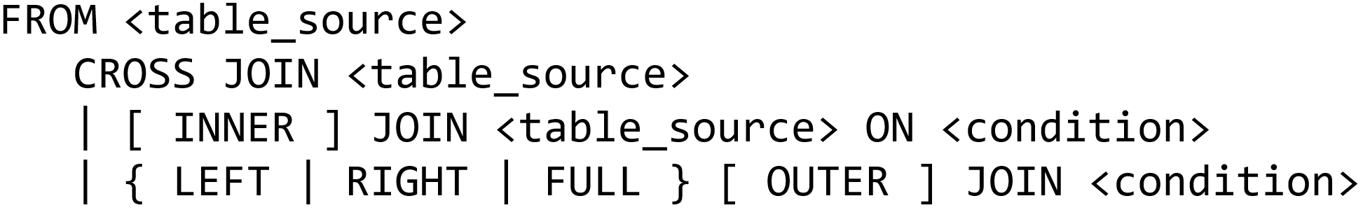
Welcome back everyone, this video, we’re gonna be taking a look at our last and final type of join the outer join. So here on the slide here actually shows some of the syntax that we’ve had so far, where we have our FROM clause. And we can join two different tables, two tables to and I say table source, because it doesn’t actually have to be a table from the database, right, it could be the result of a another join as well. So a table of some kind, joined with another table. So we’ve done the cross join, and we’ve done the inner join. And now we are going to do this outer join. This is this last syntax here. So we have a left, right or full outer join. And again, outer is going to be an optional key word, depending on ancy 89, or 92 syntax. But I’m going to encourage that outer be listed there, because it makes your queries significantly easier to read. But let’s take a look at what the OUTER JOIN actually contains with. So an outer join has three logical processing phases, instead of to write. So let’s take a look at what that what that looks like. So we have the Cartesian product, just like what we have with just like what we have with the cross join. And then just like the inner join, we Filter Rows out based off of some predicate. But in addition to that, we can now we now add rows from the preserved table. So what in the world is the preserve table? So fine line here is that the OUTER JOIN is just like an inner join, except with this extra third, this third processing step. So the reserved table is identified by either left, so the left table is preserved, right, or the right table is preserved or full. Both tables are preserved with us. And I’ll cover some more examples of this. Because this initially is kind of weird, like, what do I mean by a table being preserved? Well, I’ll explain that here in just a moment.

Really, we have, again, SQL 89, and 92 syntax, but really, only 92 is going to work in our current version of SQL Server. So having the outer word included there, let’s take a look at some of these joints. So a left join, it looks actually very similar to an inner join instead of although instead of just the this triangle symbol, we now have a tail on whichever side is preserved. So Table A is going to be the table that’s actually preserved. So join table A with Table B. And what do we get as a result? Well, before when we just did an inner join, we only had Kim analysis, right? So first step is cross join. So we have Jim paired with pickles, fish and ice cream, Kim pickles, fish and ice cream and Alice pickles, fish and ice cream. And then we filter based off of the ID. So only the records where the ID matches are kept. So that leaves us with two rows. But then we have a third processing step. So the third processing step is going to then add in the table the rows from the preserved table. So what does that end up with? Well, I get Kim and Alice, which is just like my original inner join. But then I also get gym added back in to the results. Because since I’m doing a Left Outer Join, rows that were not originally matched with the inner join are preserved and the result of the query.

And now you see that I have b.id and food. So B ID is from Table B and food is also from Table B. But those have no values for Jim because Jim net didn’t originally match with any record in table B. And so therefore, even though Jim has preserved in the in the query results, we don’t actually get any values from Table B because again right we had no match for Jim. So, this is the essence of the outer join, and particularly what I mean by a table being preserved. So a the preserve table, whether it be left or the right or both. records that do not have a match from the inner join step will be added back into the query at the end and columns were the the record had no matches for will be no. But let’s take a pause here and take a look at a couple of examples for the left outer join. So I do want to just highlight a couple things just to kind of show just to show the results here. So we have a couple things here, I wanted to show how many customers we actually have so that we have 663 customers in total in our database. And then we also, we also have two different buying groups. And this is important, because I’m going to start to expand this out by joining these two tables together. And so if I cross joined these two, right, it’s essentially the number of rows in table A times the number of rows in table B, and so 663 times two, right?

So if we run this query, aha, so now we get all all all of that. So 13 101 101,326 rows, okay, so each of the buying groups paired with all of the customers. So that is, that’s a lot, right. And that’s not necessarily valid data, it doesn’t really necessarily showcase the relationship between the two. But if we change this to an inner join, instead of just a cross join, okay. So again, right, I’m kind of just showcasing the each of the each of the logical processing steps, right, you can see step one, by you doing just a cross join, you can do, you can see the result of step two by doing just in just the inner join. So with just the inner join, I only get the customers whose buying group matches the customer buying group. And so now I only have 402 rows, right? So only the customers who have a buying group in the buying group table. Now, what if I change this to an outer join? So instead of enter, I’m going to say left. So now what happens?

So if I run this, I had 400. Before. Now I have 663. Again, right? Now I have 663. Again, because right? Because my sales customers is the preserved table, I keep all of the customers. And then I have all the customers who had a match are paired with the record inside of the buying group table. So if we go back over here, and go to the results, if I scroll down aways, let’s see here. Yep, scroll. Scroll down aways here. Now we have all the customers who are not associated with a buying group. So let’s say in this case, these customers aren’t associated with a big company. They’re just, you know, your normal person that is placing some orders for us. But this is the power of what a Left Outer Join can actually achieve. Okay, so one way we can actually identify which which customers are added, so the customers that were added, or the customers who don’t have a buying group. And so we can we can actually figure out the exact same the those exact people by just filtering out those who are no, so were big, buying group and big buying group is no, so the the customers who were not able to be paired with a buying group, those are only those customers. So we have 261 rows, right.

So we had, we had 400 customers who were paired with the buying groups, and then 260, who were not another way to do this is actually adding this based off of the bind group. So we can leave it just as the left outer join. But I’m going to introduce something that’s a little bit more useful as far as the LEFT JOIN goes. So this down here is relatively the same. But now I’m going to actually join a group by the buying group. That way all of the customers with that are associated with buying group, the first one or the second one, so we should have, remember we have to bind groups. So we should have two records as associate two records as a result of this. But remember, the is no function. So that’s going to check if this group Is No, if this column is no, then it’s going to replace no with no buying group, which is a lot more user friendly than saying just no as a result of the table. So this is an extremely useful function to actually have. But let’s give this query run, see what the result is. Haha. So we actually ended up with three buying groups instead of just two. So here are our two original buying groups. And then our third group is the knoll group, right. And remember, when we do a group buy, or aggregates, no oil is treated as the same value. So all no values are considered equivalent. So when we do the group by all Knowles are grouped into the same group, okay, since we’re grouping by buying group, and that’s no, all those who don’t have a buying group get put into that, that no buying group category. So this is pretty useful. Let’s see, though how many customers for each customer category.

But in order to get to the customer category, I’m actually going to need to introduce a right join. So let’s flip back real quick, and see an example of what the right join looks like. So a Right Outer Join, like my symbol here is flipped, right, so the tail is on the right hand side, meaning that the right table table B is going to be the table that’s actually preserved. So Table B will be preserved here. And so I still get Kim and Alice, remember, that’s the result of my inner join. Because Kim, the IDS two and three match with the IDS two and three, and Table B. But now ice cream has no pairing, right. And so the right side of the table, right seven and ice cream are preserved. And the left side where the the a.id, and name are get null out. So they are left out because they have no match. So Jim is not included here and the RIGHT OUTER JOIN, because Table B is preserved instead, instead of Table A. So let’s take a look at an example here. So our right join. I want to see how many customers we have for each category. And so I have this table, let’s actually add this to a second line here. So it’s easier to read. So we have select Customer category ID and category name. And see this is not buying group analysis customer category. But we have count star customer count. And so we have from sales customers, right join sales dot customer categories, on customer category, Id grouped by the category ID and then order by order by the ID. So if we run this, there we go. We have eight rows, so eight customer categories with the customer count.

And each one. We have these weird records here. We have one customer for agent and wholesaler and one for general retailer. So this is kind of weird. Do we actually have one customer in those categories? Or right? Since we have a right join, right, we’re right join on customer categories. And so categories are preserved. So we get all of the categories. But if a category has no customers, the customers are No. and No is still included in account. So we need to do count star, the noise actually kept in play. So we have some unused categories. So we can find those unused categories by changing this out. Let me put this on another line again, we can change this out and add the where customer ID is no. And so if I execute this query, we see those same three categories that how we had one customer and then our have no customer ID associated with them when we do the right join. So how do we correct our queries so that we show zero for the account instead of missing that out? So let’s bring this query back. So here is our query that we had earlier. So we had our count, and here are those three agent, wholesaler and general retailer, all those should have zero customers. Well, instead of counting star counting star will actually force the aggregate to include Knowles by default.

But we can say, See customer ID here instead. And run this query. Ah, now we get truly zero as a result, so count star is going to count the number of rows in the result right in the end that in each group, count customer ID, if you specify the column you want the count, we’ll count the number of non null values, which is an extremely useful, useful tool to make it to do a distinction between. And this is even more important as we start doing left and right and full outer joints. But we can, we can flip this, if we want to do a left join. Right, a left join will actually exclude all the customer categories that don’t match. But if we actually change, just to highlight how the direction now matters with our outer joins, if I’ve switched these two, it’s equivalent to the previous right outer join that we had earlier. But that is the left and right outer join. But if we can do a left outer join, and a right or outer join, we can also do a full outer join. So the FULL OUTER JOIN is going to preserve both tables. So we have tails on both ends now have our symbol there. So a table a full outer join table B. And so we get as a result, right, Kim and Alice, those are the two that have a full set of records, because those are the only two that matched in the inner join. But now we have Jim, on the left, right, because so the the result have a left outer join, and the results of the right outer join. So seven and ice cream are also included.

And you can kind of see the different null values there. But a Full Outer Join is nothing more than the result of a Right Outer Join, and the result of a left outer join. So the preservation step anyways. But let’s take a look at an example of the full outer join. So let’s plot this query. And here is it a run. So just kind of showcasing what this actually is here. So we have color names, stock items, stock item name, now we’re working with the warehouse table. And we’re doing a full join on stock items. On color ID equals color ID order by color ID order by stock ID. And so here, we see we have a bunch of no records. And then if we scroll down enough, we see here’s the two. So all the records up here, that’s the result of the left join. Here’s the right join. And then here are all the records that actually had both so they had to match a color and a stock stock item name. Now, stock item. In general, if talking about the relationship between the table a stock items has a knowable foreign key to the colors table. So and we also have colors that are unused by stock items, right? So imagine have a whole bunch of different colors. And we may not actually have a an item that is that color.

So that is the end kind of the end result of our full outer join. So again, right, a left join is going to preserve the left table, a right join is going to preserve the right side of the join, and then a full preserve both. So just kind of remember highlighting here in general, with all of our difference joins that we’ve covered so far, we have the cross join, which is the all combinations of rows between the two tables, that’s the base join that we’re working off of the inner join adds to the cross join a filter. So give me only the rows that have a match on this particular predicate. So Column A equals column B and so on and so forth. And then when we can also do a OUTER JOIN, which adds a present Step, and the table that is actually preserved is going to be either the left table in the left outer join the right table in the RIGHT OUTER JOIN, or both in case of a full outer join. But that covers the gist of most of the joins we’ll be covering for this class. But we’ll be utilizing joins in a variety of different ways moving forward into into some more complicated queries at any end. But I’m going to stop the video here. If you please feel free to reach out if you have questions.