CC 520 Syllabus - Spring 2024

• Link to this Syllabus
• Previous Versions

Contact

Professor: Josh Weese – weeser@ksu.edu

• Office: 2214 Engineering Hall (DUE)
• Phone: Office - (785) 317-3353
• Office Hours: See my calendar . Office hours are always available online and in-person. For online help during office hours, please send a direct message in MS Teams (busy times will utilize https://officehours.cs.ksu.edu/ ).
  • Want to meet with me outside office hours? https://calendly.com/weeser

Prerequisites

• CC 315 - Data Structures & Algorithms II
• CC 410 - Advanced Programming (Prerequisite or Concurrent Enrollment)
• Optional: MATH 312 - Finite Applications of Mathematics or MATH 510 - Discrete Mathematics

Recommended Texts

These books are not required. I will be providing notes, videos, and walk through examples during the course. If you are looking for more traditional text-book material, I have found these books to be helpful.

• T-SQL Fundamentals (Third Edition) by Itzik Ben-Gan
• Database Systems: The Complete Book (Second Edition) by Hector Garcia-Molina, Jeffrey D. Ullman, Jennifer Widom
• SQL Success - Database Programming Proficiency by Stephane Faroult

Required Software

We will be utilizing MS SQL Server for this course. For information about accessing SQL Server for the course, see SQL Server Access .

How to Get Help in this Course

CC 520 Database Essentials is not like your standard programming course. We will be doing some programming, but our focus will be primarily with data; how to store it, retrieve it, manipulate it, and use it with an application. Some of the topics we will cover are easier than others, but some can be fairly tricky. That, coupled with this being an online course, you are encouraged to seek help whenever you feel you are being overwhelmed or don’t understand a topic. You are not alone! We will always be willing to help students with any questions you may have about the class or other issues related to Computing Science. So please, don’t be afraid to ask questions. Get help early and often!

Here are the 5 recommended ways to get help in this course:

• Review the course materials posted on K-State Canvas and the course website
• Check the Edstem Discussion board to see if a similar question has been asked, otherwise, post a new question.
• Visit your professor’s office hours, or the office hours for your TA if available
• Send a message to the CIS 520 Help email (cc520-help@KSUemailProd.onmicrosoft.com )).
• Ask your teammates for help or advice on assignments or projects (be mindful of the honor code!)
• Schedule a one-on-one meeting with your professor/TA

More on the Edstem Discussion board

This semester, we will be using edstem.org, specifically, there Ed Discussion platform. Ed Discussion is a reddit/forum style web app that allows students to post and ask questions. This will be our preferred way of communication when it comes to questions/etc. in the course. Please adhere to the following guidelines:

• Before creating a new thread, please make sure there isn’t a similar one already made.
• If you are asking a question in Ed Discussion, please correctly mark it as such along with the correct tags.
• Please make your thread public when possible in case others have the same questions.
  • Threads can be made anonymous when needed. Course staff may anonymize private threads and make them public if they find it to be beneficial for the class.
• When posting code, please do not post solutions or part of solutions to homework. If you need to share your code with us, please make your thread private.
• If you would like a new category or tag made, please let us know!

If you need help getting started with the platform, please go through the following links:

• Student guide to Ed Discussion
• Content Editor Guide
• Push Notifications

Course Overview

Introduction to concepts and techniques in database management. Overview of relational databases, NoSQL databases, and related topics. Database programming and use of databases in applications. Theory and architecture of database management systems (DBMS).

Course Description

The purpose of this course is to introduce concepts, approaches, and techniques in database management. This includes exploring the representation of information as data, data storage techniques, foundations of data models, data retrieval, database design, transaction management, integrity and security.

Student Learning Outcomes

After completing this course, a successful student will be able to:

• Write and read SQL, including queries, relations, database modifications, constraints, triggers, transactions, and views.
• Recognize the difference between NoSQL and its philosophy compared to SQL.
• Design and create databases utilizing entity relationship models, functional dependencies, and normalization.
• Design queries and databases that are optimized in storage, retrieval, and processing of data.
• Create an application that utilizes a database.

Major Course Topics

• SQL Language
• NoSQL & its relation to SQL
• DBMS design
• Programming with databases
• Database system architecture
• Database efficiency
• Practical applications of databases

Course Structure

This course is being taught 100% online. There may be some bumps in the road as we refine the overall course structure. Students will work through each set of modules, with weekly or bi-weekly due dates. Material will be provided in the form of recorded videos, links to online resources, and discussion prompts. Each module will include a hands-on assignment, which will be graded interactively by the instructor. Assignments may also include written portions or presentations, which will be submitted online.

Grading

There will be three exams for the course. Students will be evaluated based on exams, homework assignments, and a term project. Assignments are to be completed without any collaboration with classmates or other outside help unless otherwise stated. Any unauthorized aid may result in a 0 for the assignment or an XF for the course and a report submitted to the Academic Honor Council. All assignments will be submitted through Canvas. The specific grading scheme is shown below:

• Exams/Quizzes: 35%
• Homework assignments: 25%
• Final Project: 40%

Assignments

In order to avoid turning in code or SQL that does not work (or maybe even the wrong file) please double check your solution after you submitted it to Canvas. Redownload what you submitted from Canvas and run it again to assure that the program you submitted is working as intended.

Late Work

Every student should strive to turn in work on time. Late work will receive penalty of 10% of the possible points for each day its late. Some assignments will NOT be accepted late! Others will be limited to a maximum of three days late (not always 3 days). Note that this penalty is applied on a per hour basis (i.e. if your assignment is 12 hours late, it will receive a ~5% deduction)

Subject to Change

The details in this syllabus are not set in stone. Due to the flexible nature of this class, adjustments may need to be made as the semester progresses, though they will be kept to a minimum. If any changes occur, the changes will be posted on the K-State Canvas page for this course and emailed to all students.

Safe Zone Statement

I am part of the SafeZone community network of trained K-State faculty/staff/students who are available to listen and support you. As a SafeZone Ally, I can help you connect with resources on campus to address problems you face that interfere with your academic success, particularly issues of sexual violence, hateful acts, or concerns faced by individuals due to sexual orientation/gender identity. My goal is to help you be successful and to maintain a safe and equitable campus.

Standard Syllabus Statements

Academic Honesty

Kansas State University has an Honor and Integrity System based on personal integrity, which is presumed to be sufficient assurance that, in academic matters, one’s work is performed honestly and without unauthorized assistance. Undergraduate and graduate students, by registration, acknowledge the jurisdiction of the Honor and Integrity System. The policies and procedures of the Honor and Integrity System apply to all full and part-time students enrolled in undergraduate and graduate courses on-campus, off-campus, and via distance learning. A component vital to the Honor and Integrity System is the inclusion of the Honor Pledge which applies to all assignments, examinations, or other course work undertaken by students. The Honor Pledge is implied, whether or not it is stated: “On my honor, as a student, I have neither given nor received unauthorized aid on this academic work.” A grade of XF can result from a breach of academic honesty. The F indicates failure in the course; the X indicates the reason is an Honor Pledge violation.

For this course, a violation of the Honor Pledge will result in sanctions such as a 0 on the assignment or an XF in the course, depending on severity. Actively seeking unauthorized aid, such as posting lab assignments on sites such as Chegg or StackOverflow, or asking another person to complete your work, even if unsuccessful, will result in an immediate XF in the course.

This course assumes that all your course work will be done by you. Use of AI text and code generators such as ChatGPT and GitHub Copilot in any submission for this course is strictly forbidden unless explicitly allowed by your instructor. Any unauthorized use of these tools without proper attribution is a violation of the K-State Honor Pledge .

We reserve the right to use various platforms that can perform automatic plagiarism detection by tracking changes made to files and comparing submitted projects against other students’ submissions and known solutions. That information may be used to determine if plagiarism has taken place.

Students with Disabilities

At K-State it is important that every student has access to course content and the means to demonstrate course mastery. Students with disabilities may benefit from services including accommodations provided by the Student Access Center. Disabilities can include physical, learning, executive functions, and mental health. You may register at the Student Access Center or to learn more contact:

• Manhattan/Olathe/Global Campus – Student Access Center
  • accesscenter@k-state.edu
  • 785-532-6441
• K-State Salina Campus – Julie Rowe; Student Success Coordinator
  • jarowe@k-state.edu
  • 785-820-7908

Students already registered with the Student Access Center please request your Letters of Accommodation early in the semester to provide adequate time to arrange your approved academic accommodations. Once SAC approves your Letter of Accommodation it will be e-mailed to you, and your instructor(s) for this course. Please follow up with your instructor to discuss how best to implement the approved accommodations.

Expectations for Conduct

All student activities in the University, including this course, are governed by the Student Judicial Conduct Code as outlined in the Student Governing Association By Laws , Article V, Section 3, number 2. Students who engage in behavior that disrupts the learning environment may be asked to leave the class.

Mutual Respect and Inclusion in K-State Teaching & Learning Spaces

At K-State, faculty and staff are committed to creating and maintaining an inclusive and supportive learning environment for students from diverse backgrounds and perspectives. K-State courses, labs, and other virtual and physical learning spaces promote equitable opportunity to learn, participate, contribute, and succeed, regardless of age, race, color, ethnicity, nationality, genetic information, ancestry, disability, socioeconomic status, military or veteran status, immigration status, Indigenous identity, gender identity, gender expression, sexuality, religion, culture, as well as other social identities.

Faculty and staff are committed to promoting equity and believe the success of an inclusive learning environment relies on the participation, support, and understanding of all students. Students are encouraged to share their views and lived experiences as they relate to the course or their course experience, while recognizing they are doing so in a learning environment in which all are expected to engage with respect to honor the rights, safety, and dignity of others in keeping with the K-State Principles of Community .

If you feel uncomfortable because of comments or behavior encountered in this class, you may bring it to the attention of your instructor, advisors, and/or mentors. If you have questions about how to proceed with a confidential process to resolve concerns, please contact the Student Ombudsperson Office . Violations of the student code of conduct can be reported using the Code of Conduct Reporting Form . You can also report discrimination, harassment or sexual harassment , if needed.

Netiquette

Online communication is inherently different than in-person communication. When speaking in person, many times we can take advantage of the context and body language of the person speaking to better understand what the speaker means, not just what is said. This information is not present when communicating online, so we must be much more careful about what we say and how we say it in order to get our meaning across.

Here are a few general rules to help us all communicate online in this course, especially while using tools such as Canvas or Discord:

• Use a clear and meaningful subject line to announce your topic. Subject lines such as “Question” or “Problem” are not helpful. Subjects such as “Logic Question in Project 5, Part 1 in Java” or “Unexpected Exception when Opening Text File in Python” give plenty of information about your topic.
• Use only one topic per message. If you have multiple topics, post multiple messages so each one can be discussed independently.
• Be thorough, concise, and to the point. Ideally, each message should be a page or less.
• Include exact error messages, code snippets, or screenshots, as well as any previous steps taken to fix the problem. It is much easier to solve a problem when the exact error message or screenshot is provided. If we know what you’ve tried so far, we can get to the root cause of the issue more quickly.
• Consider carefully what you write before you post it. Once a message is posted, it becomes part of the permanent record of the course and can easily be found by others.
• If you are lost, don’t know an answer, or don’t understand something, speak up! Email and Canvas both allow you to send a message privately to the instructors, so other students won’t see that you asked a question. Don’t be afraid to ask questions anytime, as you can choose to do so without any fear of being identified by your fellow students.
• Class discussions are confidential. Do not share information from the course with anyone outside of the course without explicit permission.
• Do not quote entire message chains; only include the relevant parts. When replying to a previous message, only quote the relevant lines in your response.
• Do not use all caps. It makes it look like you are shouting. Use appropriate text markup (bold, italics, etc.) to highlight a point if needed.
• No feigning surprise. If someone asks a question, saying things like “I can’t believe you don’t know that!” are not helpful, and only serve to make that person feel bad.
• No “well-actually’s.” If someone makes a statement that is not entirely correct, resist the urge to offer a “well, actually…” correction, especially if it is not relevant to the discussion. If you can help solve their problem, feel free to provide correct information, but don’t post a correction just for the sake of being correct.
• Do not correct someone’s grammar or spelling. Again, it is not helpful, and only serves to make that person feel bad. If there is a genuine mistake that may affect the meaning of the post, please contact the person privately or let the instructors know privately so it can be resolved.
• Avoid subtle -isms and microaggressions. Avoid comments that could make others feel uncomfortable based on their personal identity. See the syllabus section on Diversity and Inclusion above for more information on this topic. If a comment makes you uncomfortable, please contact the instructor.
• Avoid sarcasm, flaming, advertisements, lingo, trolling, doxxing, and other bad online habits. They have no place in an academic environment. Tasteful humor is fine, but sarcasm can be misunderstood.

As a participant in course discussions, you should also strive to honor the diversity of your classmates by adhering to the K-State Principles of Community .

Discrimination, Harassment, and Sexual Harassment

Kansas State University is committed to maintaining academic, housing, and work environments that are free of discrimination, harassment, and sexual harassment. Instructors support the University’s commitment by creating a safe learning environment during this course, free of conduct that would interfere with your academic opportunities. Instructors also have a duty to report any behavior they become aware of that potentially violates the University’s policy prohibiting discrimination, harassment, and sexual harassment, as outlined by PPM 3010 .

If a student is subjected to discrimination, harassment, or sexual harassment, they are encouraged to make a non-confidential report to the University’s Office for Institutional Equity (OIE) using the online reporting form . Incident disclosure is not required to receive resources at K-State. Reports that include domestic and dating violence, sexual assault, or stalking, should be considered for reporting by the complainant to the Kansas State University Police Department or the Riley County Police Department . Reports made to law enforcement are separate from reports made to OIE. A complainant can choose to report to one or both entities. Confidential support and advocacy can be found with the K-State Center for Advocacy, Response, and Education (CARE) . Confidential mental health services can be found with Lafene Counseling and Psychological Services (CAPS) . Academic support can be found with the Office of Student Life (OSL) . OSL is a non-confidential resource. OIE also provides a comprehensive list of resources on their website. If you have questions about non-confidential and confidential resources, please contact OIE at equity@ksu.edu or (785) 532–6220.

Academic Freedom Statement

Kansas State University is a community of students, faculty, and staff who work together to discover new knowledge, create new ideas, and share the results of their scholarly inquiry with the wider public. Although new ideas or research results may be controversial or challenge established views, the health and growth of any society requires frank intellectual exchange. Academic freedom protects this type of free exchange and is thus essential to any university’s mission.

Moreover, academic freedom supports collaborative work in the pursuit of truth and the dissemination of knowledge in an environment of inquiry, respectful debate, and professionalism. Academic freedom is not limited to the classroom or to scientific and scholarly research, but extends to the life of the university as well as to larger social and political questions. It is the right and responsibility of the university community to engage with such issues.

Campus Safety

Kansas State University is committed to providing a safe teaching and learning environment for student and faculty members. In order to enhance your safety in the unlikely case of a campus emergency make sure that you know where and how to quickly exit your classroom and how to follow any emergency directives. Current Campus Emergency Information is available at the University’s Advisory webpage.

Student Resources

K-State has many resources to help contribute to student success. These resources include accommodations for academics, paying for college, student life, health and safety, and others. Check out the Student Guide to Help and Resources: One Stop Shop for more information.

Student Academic Creations

Student academic creations are subject to Kansas State University and Kansas Board of Regents Intellectual Property Policies. For courses in which students will be creating intellectual property, the K-State policy can be found at University Handbook, Appendix R: Intellectual Property Policy and Institutional Procedures (part I.E.) . These policies address ownership and use of student academic creations.

Mental Health

Your mental health and good relationships are vital to your overall well-being. Symptoms of mental health issues may include excessive sadness or worry, thoughts of death or self-harm, inability to concentrate, lack of motivation, or substance abuse. Although problems can occur anytime for anyone, you should pay extra attention to your mental health if you are feeling academic or financial stress, discrimination, or have experienced a traumatic event, such as loss of a friend or family member, sexual assault or other physical or emotional abuse.

If you are struggling with these issues, do not wait to seek assistance.

• Kansas State University Counseling and Psychological Services offers free and confidential services to assist you to meet these challenges.
• Lafene Health Center has specialized nurse practitioners to assist with mental health.
• The Office of Student Life can direct you to additional resources.
• K-State Family Center offers individual, couple, and family counseling services on a sliding fee scale.
• Center for Advocacy, Response, and Education (CARE) provides free and confidential assistance for those in our K-State community who have been victimized by violence.

For Kansas State Salina Campus:

• Kansas State Salina Counseling Services offers free and confidential services to assist you to meet these challenges.
• The Kansas State Salina Office of Student Life can direct you to additional resources.
• The Kansas State Salina Campus offers several services for students, including health services, counseling, and academic assistance.

For Global Campus/K-State Online:

• K-State Online students have free access to mental health counseling with My SSP - 24/7 support via chat and phone.
• The Office of Student Life can direct you to additional resources.

University Excused Absences

K-State has a University Excused Absence policy (Section F62) . Class absence(s) will be handled between the instructor and the student unless there are other university offices involved. For university excused absences, instructors shall provide the student the opportunity to make up missed assignments, activities, and/or attendance specific points that contribute to the course grade, unless they decide to excuse those missed assignments from the student’s course grade. Please see the policy for a complete list of university excused absences and how to obtain one. Students are encouraged to contact their instructor regarding their absences.

Face Coverings

Kansas State University strongly encourages, but does not require, that everyone wear masks while indoors on university property, including while attending in-person classes. For additional information and the latest updates, see K-State’s face covering policy .

Copyright Notification

Copyright 2023(Joshua L. Weese) as to this syllabus and all lectures. During this course students are prohibited from selling notes to or being paid for taking notes by any person or commercial firm without the express written permission of the professor teaching this course. In addition, students in this class are not authorized to provide class notes or other class-related materials to any other person or entity, other than sharing them directly with another student taking the class for purposes of studying, without prior written permission from the professor teaching this course. The digital materials included here come with the legal permissions and releases of the copyright holders. These course materials should be used for educational purposes only; the contents should not be distributed electronically or otherwise beyond the confines of this online course. The URLs listed here do not suggest endorsement of either the site owners or the contents found at the sites. Likewise, mentioned brands (products and services) do not suggest endorsement. Students own copyright to what they create.

MS SQL Server Access

In order to complete homework assignments and practice on your own, you will need access to SQL Server. Your access requires a client tool and a server.

Client Tools

For this course, you will need to use a SQL client tool to access a SQL Server instance.

• All resources are available via remote access on remote.cs.ksu.edu. See https://support.cs.ksu.edu/CISDocs/wiki/Remote_Access for more information on how to utilize the remote resources.
• If you do not have a CS account, one can be requested here: https://selfserv.cs.ksu.edu/
  • To reset a forgotten password (or unlock an accound after too many failed login attempts), see https://password.cs.ksu.edu/
• We will be using two client tools throughout the semester. It is highly encouraged to also install a client on your own computer.
  • Azure Data Studio - Windows, macOS, or Linux: https://docs.microsoft.com/en-us/sql/azure-data-studio/download
  • SQL Server Management Studio (aka SSMS) - Windows Only: https://docs.microsoft.com/en-us/sql/ssms/download-sql-server-management-studio-ssms
• Windows Computer Labs: All Windows workstations in the Computer Science department have these client tools available.

Database Server

A database server is needed to host a database. In this course, we will use Microsoft SQL Server.

Option 1: Provided Database Server

Using the following information, you connect to our SQL Server instance from one of the aforementioned client tools. Depending on the tool, not all of this information may be requested. If you are accessing from your own computer, you will need to connect to the campus network via VPN first.

• Server Type: Database Engine
• Server Name: mssql.cs.ksu.edu
• Authentication Type: SQL Server Authentication
• Login: Your eID
• Password: Instructor will provide your initial password, then you will be prompted to change it.

Once connected, we will most often use the database WideWorldImporters. You should also have a database named after your EID that you can utilize to explore other examples.

Option 2: Install Your Own

Installing your own copy of Microsoft SQL Server is highly encouraged. Most versions of SQL Server will work for this course…but I recommend the one below for a lightweight option (the full version of MS SQL Server is not needed for this course and can take up quite a bit of resources when installed).

• MS SQL Server Express: A light-weight server that is often used for local development. It is an installation option of SQL Server Express Edition.

  1. You can install SQL Server Express here: SQL Server Express 2019 . The “Basic” installation option is sufficient.

     1. Alternatively, you can install LocalDB. For more information, see https://docs.microsoft.com/en-us/sql/database-engine/configure-windows/sql-server-express-localdb . This runs with even a smaller footprint than Express. If you go with this option, you will use a different server name to connect below in step 2: (localdb)\MSSQLLocalDb

  2. Now you can run one of the above client tools to connect to your local instance of SQL Server. You need to use the following information to connect in a query window:

     • Server Type: Database Engine
     • Server Name: localhost\SQLEXPRESS
     • Authentication Type: Windows Authentication

  3. Install the WideWorldImporters database. It it is hosted on github.com . For for our use, you can download the WideWorldImporters-Standard.bak copy of the database. Once the backup file is downloaded, move it to your user directory and issue the following SQL to restore the backup:

  RESTORE DATABASE [WideWorldImporters]
  FROM DISK = N'THEPATH\WideWorldImporters-Standard.bak'
  WITH FILE = 1,
  MOVE N'WWI_Primary' TO N'THEPATH\WideWorldImporters.mdf',
  MOVE N'WWI_UserData' TO N'THEPATH\WideWorldImporters_UserData.ndf',
  MOVE N'WWI_Log' TO N'THEPATH\WideWorldImporters.ldf';

• Docker Container Option: A full-featured database engine running in a Linux container. To build your own image, the container and the sample database are both installed by following the steps of the online Microsoft article Restore a SQL Server database in a Linux Docker container . Walk through the steps described until you complete the section of the online article named Verify the restored database .

Database Overview

Overview

Databases are essentially everywhere with modern technology. We live in a digital age, far more connected online than ever, and utilizing a number of smart devices that generate thousands of data points just for a single person. Our digital foot print is always growing…even more so for companies that are able to store far more data than they used to about their operation. Almost every application or smart device we use is connected to some form of database to store information it creates/collects.

The before times… Databases allow us to manipulate and store information significantly faster and in much larger volumes than ever before. But before databases existed, of course we had classic paper filing systems. Though, even when we started to advance technologies and created digital computers, data still was not readily accessible at our fingertips in large amounts. A lot of data was stored in single or multiple files like text files on computers for quite some time. File-based data storage and access is difficult to work with, resulting in a tediously written programs that resulted in a lot of repeated code. Data integrity, retention, and access also presents a major issue, particularly when more than one device/program/person needs to work the with data at the same time.

The main concept behind a database is a centralized data store that manages data integrity and allows fast retrieval and manipulation of data. Initially, when the idea of a data store or database was materialized, they weren’t really that much better than a normal file store. They were typically a static system in the 1960’s, which meant that modifications were tedious and hard to complete. More so, programmers had to know the physical structure of the database in order to utilize the data.

Edgar F. Codd

In 1970, Edgar F. Codd , a researcher at IBM published the paper A Relational Model of Data for Large Shared Data Banks. In this paper, he outlines how database systems could utilize mathematical foundations in set theory, predicate logic, and relational algebra. This work led to the creation of some of the first relational databases as well as the language used to work them called the Structured Query Language (SQL ). We will be re-visiting some of Codd’s work throughout this course!

What is a Database?

Example Data

Here we can see some basic information about universities in a table. Much of the data we use in relational databases resemble this format, except the information is typically at a much larger scale. A lot of situations find this data being stored in spreadsheets, comma separated value (csv) files, and alike; however, these formats have limited capability in manipulating and storing data. Spreadsheet applications can do some of this type of work, but there are limits…particularly in terms of scalability, accessibility, and reliability. That is where relational databases come into play!

Operations

In mathematics, when we perform operations on numbers, we get numbers as a result. So in databases, when we perform operations on datasets, we can get new datasets as a result. The vast majority of operations we perform on a database will be done in the form of a query. Think of a query as a question that we would like answered about some data or entity. The word entity can be used to describe a single record about something contained in a database, like one single student record. We can extract entities using a query with three primary database operations: selection, projection, and join.

• Selection is used to extract a specific subset of rows that match a certain predicate (condition). This operation acts like a filter for querying data. The highlighted rows below are from selecting universities where the ‘Year Established’ is on or before 1863.

• Projection is used to extract a specific subset of columns. This operation chooses which parts of the data are used. The columns that are chosen based off of the provided column names. The highlighted columns in the table below represent the projection of the columns ‘Name’, ‘Nickname’, ‘Website’, and ‘Location’. Note that when projection is used without selection, all rows of data are included.

• Join is used to combine data from multiple datasets. There are different types of joins that we will talk about…but when tables are joined, not all data has to be included in the operation. In the example below, you can see how the ‘School’ dataset can be joined with parts of the ‘Conferences’ dataset to create a new dataset all together.

Relational Vocabulary

There are a lot of terms that are used when working with databases. Some words can be used interchangeably.

• Relations: Two-dimensional tables, each with rows and columns.

• Attributes: The columns of the relation. The attributes are a set, not a list.

• Tuples: The rows in the relation. The tuples are a set, not a list.

• Domain: An elementary type for each attribute. A value must not be a set, list, array, etc.

• Keys: A set of attributes that prevent two tuples in the relation to have the same values in all the key attributes.

• Combining the above concepts into a complete database design is the database schema.

Introduction to Tables and Constraints

Video Transcription

Welcome everyone. In this video, we’re going to take our first look into some sequels, specifically t SQL, which is Microsoft’s implementation of the SQL standard.So to start off, we’ll talk a little bit about basic table structure. We’ve talked up already in a previous lecture about general table structure, but not necessarily how we actually create that in our database. We’ll also do a basic introduction to constraints today, which includes the not null constraint, primary keys, unique keys, foreign keys, check constraints and default constraints. These are by no means all of the constraints that are possible to use in SQL, as well as SQL Server, which is the database system that we’ll be using. But this should get you a good introduction into them. And we’ll be covering and using these throughout the course.

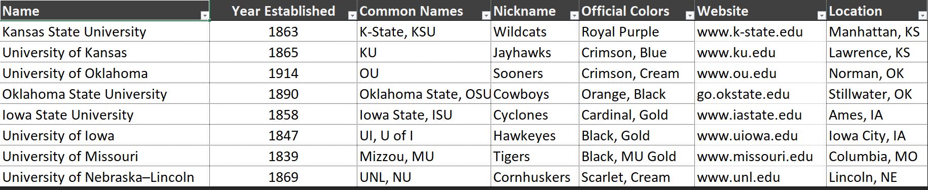
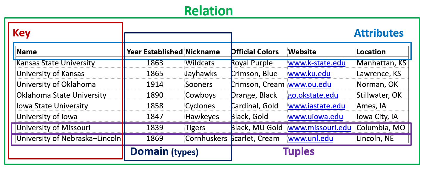
So as we noted before, tables are a physical form of a relation. Remember, relations are collections of attributes, tuples, and all of that, basically, what we saw with the university data, so the table is the physical manifestation of that. Now a table inside of your database is going to contain one or more columns, it cannot contain zero columns. So our database can’t contain a table that has no columns, it must contain at least one column, but it does not have to have rows or columns are a physical form of attributes, right. So remember, a relation is made up of attributes and tuples. Those attributes take the physical form of a column. Columns have a lot of different properties to them. Again, they are a set, not a list. So therefore, all columns inside of a table must be uniquely named right. So in this particular example, here, it would be impossible for us to have two columns called nickname, right. And so we have to have unique names for each column.

Name, all columns must also have a data type, and no ability. So whether or not that column can have data or whether or not that data is actually required. So a lot of records have inconsistent data. And some data is optional, right? When you fill out a form on the internet, or even in general, right, not all fields are typically required, depending on the situation that you have, the non required fields are allowed to be no, right. This diagram that I have here on my slide is an entity relationship diagram. This will look very similar to since you’ve encountered UML. Before, this is just the database version of that typical style of diagram. So on the left hand side, we have the indication of whether or not this column is a key, we have the individual columns listed here, the columns data type on the right, and then of course, the table name here at the top. Now also notice that we typically will also include the schema that that table belongs to remember schemas act kind of like a namespace inside of a database. So all tables for a particular database are contained inside of a schema.

And so and we’ll talk in a variety of different lectures about the individual data types here. And I’ll talk a little bit more about them. And this particular lecture as well. But we won’t get into a lot of the details just yet. But let’s take a look at some examples here on how to actually create our first table inside of our database.

So by this point, you should have watched the video and read the material on how to get Microsoft SQL Server installed, as well as as your data studio or how to reuse the remote connection in order to access an already fixed or correct installation. We’ll be using this throughout the class in order to actually write to do our exercises, or the notes that we that I showcase in lecture are in these videos. And we’ll also be utilizing this for our projects and for our homeworks but for now let’s create our first database. If this is your first time watching this video, and first time going through these examples, you will have to create your first database and the syntax or the the way we actually do that is using the Create statement, and then the name of the database that we want to create and in this case, I’m going to create a database called CC 520. And we need to also make sure that we are connected to our local installation of our database. And so in this case, I’m just going to connect to my local installation of SQL Express that is running. And then if you already have other databases in your local installation that are already created, you’ll see those pop up here.

But if you’re on your master connection here, you can actually change down here towards the bottom, you can actually change whichever database that you’re actually connecting to, just as a refresher, and if you ever want to change that connection, you can just change it up here to where it says attached to. But for now, let’s go ahead and say create, sorry, create database CC 520. So create databases, the statement, and then the name of our actual database there are remember each, just like what we do with programming each SQL statement reach query that we execute as part of our database or for our database, we need to end that with a semicolon. Now, as you’ll soon find out, not every line of SQL code will actually have a semi colon following after it. But let’s go ahead and create our database here.

So commands completed successfully. Now, keep in mind as well, if you’ve already created this database on your system, you will get an error. It says, Well, this database cc 520 already exists. So you don’t have to run this more than once. So we also need to create our first schema as part of our database as well. So just like what we did with our database above, create schema, and then we’re going to create a demo the demo schema, and then we’re going to set authorization to be DBO. We kind of hand wave over the authorization part here. This deals with permissions set for the schema, and we’ll talk about that later in the course. But for now, we just want to create this schema called demo. And note that the square brackets are TC equals or SQL servers, syntax for denoting names for database objects. Now, you can also use quotation marks here as well, quotation marks will work just the same. But the Microsoft SQL Server way of doing it would be the square brackets. Now, also note that before you actually run this create schema, we also need to make sure that we are using the correct database. Otherwise, your schema will be created in the database that whatever that your whatever your connection is actually physically attached to. And so since my connection is not connected, or directly connected to my individual database that I just created, I need to actually set use the go statement or use statements and then say, go.

So what go is going to do is it’s going to first execute this UCC 520 and then execute the Create schema. And so if I run this, both of those commands were done successfully. So this command was executed first, and then this command was executed second. Now, in theory as well, what we can do to fix this, at least as far as as your Data Studio goes, is that we can actually change our connection here. And instead of connecting to master, so we click on master first to load up all of this. And then down here for our database, we can say cc 520. Instead, press Connect. And now our connection is set to cc 520. And we don’t actually have to use the using statement or use statement to make sure we’re on the correct database.

But now that we have our basic schema and our basic database, let’s go ahead and add our first table. now. I’ll in the notes, you’ll find that I have this drop table if exists command. This is only there to if you’ve already ran through these notes. If the table exists already, you’ll get an error as a result. So as far as this example goes, you’ll want to drop the table first. So delete the table from the database. And then you can run that CREATE TABLE statement again. So let’s go ahead and do that. So we’ll do this and a couple ghosts. So drop it, drop it if it exists. And then we’re going to say create Table Table demo dot school.

So when we create table, when we create a table, the schema name needs to be included as part of the naming conventions. So that way your table, if you have more than one schema, you know which table that schema actually belongs to. So that is good practice there. So schema dot table, just like what we had with our diagram, right there. So we can see that our table name would be demo dot school. And we have each of our individual, we have each of our individual columns here. So this is the column name. Now note, I do have to put the square brackets around name here, because if I take those out, you notice that the color changes to blue. That means that it’s being recognized as a reserved word in T SQL. And so we need to either put double quotes around it or square brackets around it. So it knows that I’m intending to use it as an actual name of the column, and not part of what the reserved word represents in T SQL. And then right next to that, we’ll have our data type for the column. And then we’ll also have any constraints associated with that as well. But we’ll add those later, and in just a few minutes, but each of the columns are separated out by column as are, each of the columns are separated out by a comma, as you see here. And then again, all of those columns are wrapped inside of parentheses. And then of course, we end our SQL statement with a semi colon.

But if we run this, we see that our command is running successfully. And now I can actually browse over here into my databases. And if I refresh, I go to my cc 520, expand my tables. And now here is my demo dot school. And I can actually see all of the individual individual columns here, along with their data types associated with them. Now notice, as well, by default, if they are not, if it’s not specified, the columns are set to be not meaning that I don’t actually have to store any data for those particular columns, right? They’re nullable. And we’ll talk about the not null constraint here in just a minute. But let’s go ahead and also add some basic data associated with this. So if we look, let me go ahead and actually just touch it to the cell here. So we have inserts, which is the SQL statement to actually add more data to our data or a particular table. And we’ll talk about the insert statement later in the semester, as we get closer to that to data modification. But for now, just know that the insert statement will take a list of columns for a table, and then all of the values associated with it. So each of these row, each of these sets of parentheses are tuples, right. So this is one tuple, comma, another tuple. Remember, each tuple represents a row in our relation or table.

And each of these is in order, corresponding to each of the columns that I have up above. Now, if we run this, eight rows affected, so that means all of my eight rows of data got inserted into my table. So let us do a little bit more before we actually start moving on. So I’m going to hide this real quick. And then I’m going to…let’s go ahead and make sure our data got inserted. So I’m going to select star from demo school. Notice that my IntelliSense is thinking that demo school demo dot school does not exist. And you can safely ignore that I’m connected to the right database and I am that table is actually created, but some caching actually occurs here. And so as your Data Studio doesn’t always properly refresh right away. And so if you just created a table, and during this session, as your Data Studio may not recognize that that table actually exists yet.

But once you run that SELECT statement, so select star, and remember, select is the projection. So this picks which columns in our database that we actually want, star is a wildcard, meaning I want all of the columns. And then from is going to pick which tables I want to pull data from. And so in this case, demo dot school. But again, a lot of these SQL statements here, we’ll be covering in much more greater detail in future talks. But for now, we can see that all of our data exists in our particular table, as we inserted it just before.

So let’s take a look at a another example. So let’s move my screen just a little bit higher here. So here’s another big example. And if you want to take a pause here to type this out, now would be a really good time to pause the video to actually get this SQL code into your Azure Data Studio. Or you can copy this from the sequel notes as well. But I encourage you to start typing these out to get that muscle memory in. So just like when he first started to learn how to code, typing out SQL statements is going to be the best practice to actually get familiar with the syntax.

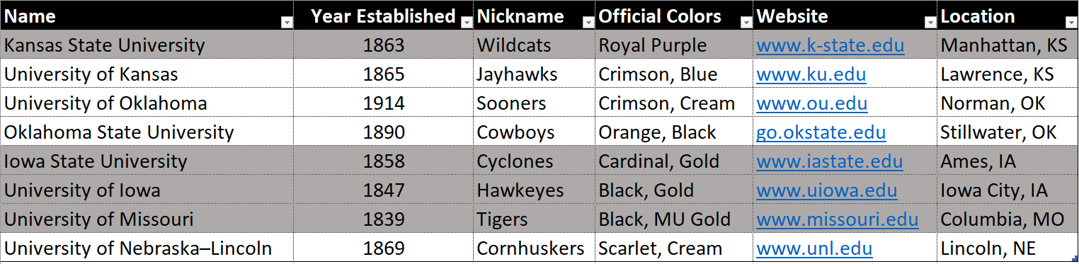
But let’s take a look at what happens here. So I had added, I added a new column here called a website, just to kind of explore here, what would happen down here in my table, so this was not included in my original table that I have up here. But it is included in this CREATE TABLE statement. But my insert has no website column. So if I run this, and then if I pull my statement from up there, and run by select star, you’ll notice that my website column all contains null values. That’s because I did not say that this website column could be or could not be no. So by default, it is normal, right? Meaning that I don’t actually have to insert data for that particular column, when I run an insert statement, I could just pick and choose which columns that I wanted.

So, but a lot of times, the vast majority of times anyways, most columns in the database would be required, so meaning they could not be not. And that’s really important, because if we have a lot of data attributes that are normal in our table, we’re actually really not being very efficient with our database design. And likewise, not being very efficient with our data storage. So it’s really important that we be very careful and allowing nullable columns. But let’s take a look at what the do what the our basic constraints could start to.

But let’s take a look at some constraints that we can use to prevent no values being inserted in our database. So constraints are essentially declarative role. So just like what we have rules and logic, we can have rules in our database as well. So our database management system, or DBMS, will check these constraints. Every time new data is added. Data is modified. And in some cases, when data is deleted, and any operation that violates a constraint will fail and return an error. So typically, this would be an exception that gets thrown. So SQL Server, our database management system will manage these constraints for us. And so when we work with our data, adding new data, deleting or modifying data, those constraints can be checked and to verify that our data or our data maintains its integrity. And that is one of the biggest reasons why we actually are using a database over something like Microsoft Excel.

But let’s take a look at our first constraint here. So as we talked about just a little bit ago, we want to make sure that We don’t have as much nor data as part of our database, right? knowable data is okay, it’s perfectly acceptable. But if we have a lot of it, our database design and storage is not that efficient. So the knowability constraint allows us to indicate which values are mandatory and which ones are not. So a value that a value is really anything that fits the domain of that column that is not null.

So in terms of a invar, char, a variable length string, that is 64 bits in length, or 64 characters in length, anything that is text or string will actually fit into that domain unless it’s no right meaning non existent. Similar thing for integers are n chars, which is a fixed length string. Again, we’ll talk about these different domain types or different data types in another class period.

Now, take a look at our ER diagram here. Now as well, we have changed a little bit of the of the structure here just a little bit, but pay really close attention to the that the name year stablish, nicknamed colors, city and state code are now a talyc. thing. So in an ER diagram, if your column name is italicized, it means that it is knowable, meaning that it is not required. If the text is not italicized, that means that column is required. So now, in this diagram, we’re making the website field required.

So let’s take a look at what that would look like in SQL. So if we recreate our table here, let’s go ahead and copy this in here. And so I know this is a lot of SQL code. But these videos would be extremely long if I sat here and typed out all of the SQL by hand, every single for every single example. So please bear with me, if you want to take some time to read through these SQL statements very carefully, please do pause the video for a moment. So you can read what’s going on here.

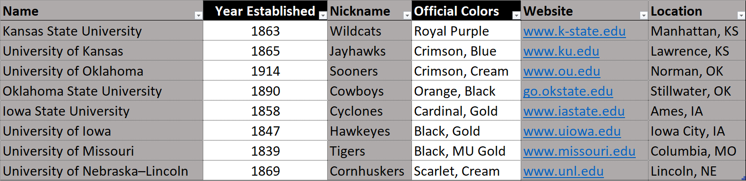
So we’re going to remove our old table. And now we’re going to create the demo duck school table again, and search the same values. And then we’re going to select everything to see what is left in it. Now keep in mind here, the change that I made is in the creation statement, I added a constraint now. And so we have our column name here, followed by our domain or column type. So this is a string that is variable length up to 128 characters. Now I am specifying that this column is not No. So by default, these columns if you do not include the knowability constraint, it by default has no in its place. And so it allows that column to be optional. But if we say not know, that column all of a sudden becomes required. So let’s go ahead and try to run this code again.

Ah, so cannot insert the value null into column website. Table cc 520 dot demo dot school column does not allow nulls insert fails, that statement has been terminated. And so when we do our select, nothing actually happens, right? Nothing is actually there inside of our table, because no data got inserted to begin with. So we have essentially restricted this. So any data that we actually try to add in our table, our database management system, SQL Server prevents us from inserting a record into the school table without the school’s website associated with it.

Now, let’s go ahead then and also make the rest of our columns not null. So here we go. And notice as well, I went ahead and took out the I went ahead and took out the website column here. But this should now work, right. But note if I ever happened to take out, let’s say one rep one value here and try to run this again. Notice that the insert fails because the number of columns for each row have to match the values up here, unlike what we had here, because we have unknowable, so we have name, year. Nickname, colors, the state, but now, right website is not included as as a column as part of my insert because I’m not actually inserting that value. So just keep in mind that that is also a restriction that we have for insertion.

But if we actually started to try to say, no here, huh, that statement has been terminated because of the error cannot insert null into the column state code, because that column does not allow nulls. And so we want to take this back. If I run this now. Everything is all good again.

All right. So these sorts of constraints may seem very simplistic at first, but especially when you have a database that is connected to a some sort of form, or anything like that is really important, as far as the database goes is to help ensure that your data is valid, ensure that your data is the data integrity actually holds up really well. A lot of times applications don’t have consistency with data. And so the database can help us enforce that consistency. Right. And again, that is one of the big reasons one of the big benefits that we are trying to leverage moving away from an Excel like file like an Excel sheet or txt file, something like that to something that is managed like a database

Key, Check, and Default Constraints

Video Transcription

Welcome back, everyone. This is part two of our introduction into tables and constraints. But now let’s start talking about key constraints. Key constraints are really important as part of our database design, because it enforces relationships and uniqueness of data throughout our individual tables. And across the relationships between those tables. Our first one here is a primary key constraint. Primary Key constraints make particular values for a column mandatory are required because a primary key uniquely identifies a row as part of an part of a table. That value being that uniquely identifies a particular record inside of a table must be unique. So we can’t have two identifiers are two values and as a primary key that are the same otherwise, we wouldn’t be able to uniquely identify a record or row in a table. And in our previous discussion, that is one of the major requirements in a relational database for table is that we must be able to uniquely identify a single tuple or row inside of a table to that primary key is really important to be unique. Also, notice here that in my ER diagram, I’ve changed a little bit of things here, the website column is gone, all of my columns here are also not italicized anymore, so everything is going to be required. And then we have our first key constraint added to our ER diagram here, PK for primary key, now more than one column can be a primary key.

So we can have a composite primary key. But for now, we’re going to shoot for just doing a primary key of school ID, which is of type Ent. But let’s take a look at a few examples here. So here’s another example of us creating a the demo dot school table. This is exactly what I have up here in my slide as well. So the new addition here is that we have a new column called school ID of type int, that cannot be null. And it is a primary key, right. So this is our primary key constraint and our not null constraint all together. And one. Also quick note here naming convention wise that we’re going here, you’ve noticed that my column, all my column names are capitalized. And then Personally, I do capital I capital D, but you may also see a lowercase D as part of this. But we have our typical insert statement down here. Notice that we do have school ID added as part of this now as well. And then school ID is listed throughout there. But if we run this, our SQL query fails, right, so invalid column name, invalid column name, school ID. So do if you are continuing on the same database that we had from our previous video, you may also have to add a go statement in between these two, or just execute these separately, because we have, we’re adding a new column here. And so our insert statement would actually fail. Since these queries are these statements are all ran on the database management system in one big batch. And again, we will talk about batch how SQL SQL Server runs queries in batches in a future video. But for now, you can run the drop and create in one in one cell in Azure Data Studio, or add the go statement in between these two.

But now if we run this, we can see that there is a violation of primary key constraint, PK school cannot insert duplicate key an object demo dot school, the duplicate key value is eight. So note that all of our key constraints are all of our constraints. inside of our SQL Server instance, for our database objects will be automatically named by SQL Server. We will talk about in a future video on how we could actually name those constraints to be a little bit more user friendly. But for now, we will use the auto generated names for them. But the reason why we have an issue here is that line 25 and line 26. Both of these tuples have the same school ID so you need University of Nebraska University of Nebraska I have the same name, same ID, but one is you when l. So University of Nebraska Lincoln, and one is University of Nebraska, Omaha. And so what we can do to fix that issue is just to say, nine here. So if we run this again, Ah, there we go. So nine rows affected. And then if we go down a little bit here and add a select star, and then from demo dot school and run that, we get our nine records out of it. Alright, so that is the basic implementation of how we would work with a primary key. Like I said, we’ll get more into more complicated keys in the future. But this gets your feet wet into some of the basics and how those primary keys actually work, and how that’s enforced when we insert data into our tables.

Now, let’s look at our next constraints. So unique constraints are very similar to how primary key constraints work. Unique constraints enforce uniqueness within that column or within those columns, it can be a composite unique key. But unlike a primary key, you can have more than one unique constraint. So this will allow this will allow Knowles inside of it as well, where a primary key cannot be no. So that is some of the primary differences between a unique key and a primary key. So we can have a composite primary key meaning that more than one column together can be the primary key. But with a unique key we can have. So for example, we could have name be unique key. And then we could also have, let’s say colors be unique or nickname be a unique key. And they could be two entirely different keys separated out with each other. But again, when we start talking more about database design and consensus consistency of data, we’ll talk a little bit more about the more complicated key constraints that we can have as part of our database. But for now, let’s just take a look at an example. So if you notice, and my ER diagram on my slide, we have the UK in the key in the key area of the diagram next to name so we’re trying to enforce unique names as part of our university table. And so what we want to do first here, let’s go ahead and do a new create statement. And again, if you get an error, you might have to add a go statement in between these. But we’re going to run the CREATE TABLE school again, primary key school ID. But now we added the unique constraint to our name. So if we run this, ah, notice that my unique, my unique key constraint was violated in our insert duplicate key and object demo dot School, which is our table, the duplicate key is University of Nebraska. So even though our primary key is not violated, the unique constraint that we have as part of our name column is because we still have this two same names University of Nebraska, and a university in Nebraska.

But what we could do is we could just add something that is a little bit more unique as part of the name University of Nebraska Lincoln, and University of Nebraska, Omaha here. And if we run this now, all nine rows were affected. And now if we run this, we can see that all of my records here are added and I correctly get University of Nebraska Lincoln and Omaha down here at the bottom. Keep in mind though, while unique keys do operate similarly to primary keys, they aren’t necessarily don’t necessarily do the exact same thing as being noted above there in the corner in our slide. And again, once we start talking about database design, and specifically normalizing our tables normalizing our information that we store in our database, we’ll get more into the harder details of why there is a big difference between these two types of PII constraints.

Alright, so then let’s take a look at our next constraint, which is check constraints. So check constraints are really cool feature inside our relational database languages, check constraints that allow us to enforce certain kinds of information for our particular columns. If you would have noticed earlier, when I’ve been doing my insert statements, we had that last row that had zero for the for the year established. So check constraints could actually enforce a particular range of data, it could can enforce a discrete set. So if we had a column we could enforce yes, no, or maybe, or yes, no, true false. And we can enforce a lot of different things here. So specific range of data, discrete values, we could also use a comparison here. So we could say, well, this column has to be between, or the end date has to be greater than or equal to the start date.

So essentially, any predicate that we can use, comparing columns of the table can be a valid check constraint. So we can use any of the columns as part of the table. And we can pretty much do any Boolean operation on those columns. That’s what we’re referring to as a predicate here. So we can do less than greater than not equal to, and, and so on. So this is a really powerful tool to verify certain, verify that our column, the data that’s being inserted into it or modified, meet certain conditions. But for now, let’s take a look at how this looks in our SQL code. And you’ll notice that I didn’t really include there’s no ER diagram here, some er diagrams, and I’ll draw some later in the class. But some er diagrams will include check constraints as part of it, but it’s not very common. But you may see them on some database design documents. But let’s see what we can do for check constraints. So the same this year, similar kind of statement that we just had before. But now we’re doing a CREATE TABLE demo dot school, and still have the unique constraint and the primary key constraint. But now what I’m actually adding here is a check constraint.

So for a year established, because we have a zero, a pesky zero down here and part of our data, so we don’t want to get an invalid year, or some really weird years. And even this, we’re I’m maxing out at your 9999. But just for a second example, we can kind of show this here. But what we’re doing here is we’re checking that the year established column. So the data that is contained inside of this column is between 1009 1999. And of course, we could put more realistic values here. But let’s go ahead and run this as an example. And so you can see that an error is generated that says that we have violated our check constraint for this particular for this particular column. So what we can do is actually create or improve our data accuracy here. So u and o was founded in 1908. So if we change that value, run it our table gets created, and all of our data gets inserted just fine. And there we have it. So there we have universe, Nebraska, Omaha with the correct date in mind. But check constraints are a very, very useful tool to enforce data integrity, data consistency, as well. Now in practice, not not all data can be cleaned this way through the database. There is some data, some data cleaning that must be done at the application level. So the tool that’s being used the to create data in certain data into the database, that tool or application recode program will need to actually do some of that data cleaning before it gets to the database. But the database management system can do some of that for you, which is a really cool thing.

Lets take a look at a another another key constraint, which is the foreign key constraint. Again, we will be talking about foreign keys throughout this class. This is just a gentle introduction. But foreign key constraints enforces what we call referential integrity. These are there are a few rules that go along with foreign keys. So foreign keys are going to just as they sound before, and so a foreign key is going to be in let’s say, table B. So table B has a foreign key. And that foreign key is going to reference a column in another table. And so the columns that are referenced must either be a primary key or a unique key name. So it can’t be just some random column, it has to be a unique inside of that particular table. So unique columns are unique keys, of course, and then primary keys which are forced to be unique in the referencing column. So the actual foreign key itself must match the type of the reference column. So the column in table B must be the same type and column A. But the constraint does work in both directions. So it’s a bi directional inference. So the referencing table is checked when the foreign key value is inserted. And when it’s updated, as well as deleted, but when when a value is deleted, and the referenced table is checked, the reference table is checked. So if a new record is inserted, the referencing table is chaps. And then vice versa for when a record is actually deleted. But this will make a lot more sense when we start looking into relationships. And we’ll talk more about foreign keys.

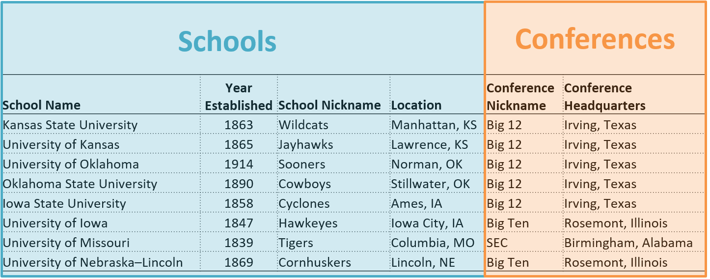
So this may be a little bit much initially. But again, we’ll be explaining this in much greater detail here in the new few near future. But this is what a foreign key constraint might look like inside of a database. And this is going to be the example that I’m going to show here. But we have demo dot school here, but we now have a new table called demo conference. And then notice here that we have a foreign key now and a school table or school table. So conference, which is a foreign key fk, and then we have a conference table. And then we have a relationship that’s drawn between these. So this is a crows foot notation to reference the, the, the relationship between these two tables, so one, so one and only one conference. So a school can be can be in one and only one conference. And a conference can be in it can be found in zero or more schools. And again, we’ll talk more about the crows foot notation in a future lecture. But just note this, this is what you’ll see for how a foreign key is referenced in the ER diagram. But again, let’s go ahead and take a look at an example because things make a little bit more sense when you actually see it in practice. So I’ll leave my diagram up there at the top corner for you. But let’s take a look at some new code here.

So this is a lot of code. But all I’m doing here is creating my demo conference table and my demo school. I have a bunch of data that’s being inserted here. And notice here that we have a foreign key constraint now in our school table. So conference, that foreign key references demo conference nickname. So references that table up there, they’ll be run this invalid name, invalid column name conference. Again, that’s because we’re doing we have batch processing issues. So the conference table must be created first. So if you’re using as your Data Studio, and using a Jupyter Notebook, you’ll need to make sure that that conferences ran first, and I’ll try to make sure that this is set up more properly in your SQL notes as well. But let’s go ahead and run this again. Ah, there we go. So five rows affected eight rows affected there. So if we run demo dot school, so all of that is and we can actually see the conference name up here now. And then if we also change this to a conference, we can actually see all of our conferences were inserted as well.

So cool, everything looks good so far. Let’s go ahead and look at how we can insert some more values. So demo dot school, inserting into school and inserting into conference. So here I am trying to insert University of Nebraska Omaha, which isn’t here yet. I took that out. We have University of Missouri University, Nebraska Lincoln, and both put them on here. And they’re going to be in the summit conference. And I’m also inserting summit into the conference table. But if I try to run this, haha, alright, so the insert statement conflicted with the foreign key constraint. School conference, the conflict occurred and the database cc 520 table demo conference column and nickname. So foreign key constraint, right. So the issue here, hey, let me for the sub summit, it does not actually. So we have you and oh here and then 1908, Mavericks, black, crimson, Omaha, everything here is the same. But this line here was not actually ran yet. So since summit and Summit League, right, because summit, if we scroll up here, the conference, right is that primary key is nickname.

And so since the summit here, did not exist when I ran this line of code, this one. So this failed, because of our foreign key constraint, we were still able to insert this into our conference table, because this executed so that’s what this one row affected down here. This one worked, but our insert did not because the summit did not exist yet. But now that it does exist, we can actually execute this in our our table gets in our value gets inserted just fine. And now when we actually run our demo dot school, University of Nebraska, Omaha is there. And then we can also pull from our conference table as well. And see that summit is there. Um, but that is the basics of how our foreign key constraints are done. But let’s go ahead and look at our next constraint thing.

Our next one here is a default constraint. Default constraints are extremely useful for information or columns that are knowable, right? So if a column is knowable, but you want data to actually be there, we can use a default value, which is really, really handy. So of course, just as it sounds, assigns a default value for a column, right, this is used on inserts when a value is not provided for that particular insult insert. So if a column is knowable, and that column is not provided as part of an insert, then a D, the default value is provided as part of the default constraint. So you can provide a value, you can still override that default value. So just because you have a default constraint does not mean that you can’t have a value insert into that column. It just means that if you don’t insert a value, the default value is actually used, I think, we can also utilize what we call an identity property that provides similar behavior. Although for an identity column, you’re not actually supposed to override those values. So that’s a little bit different. And identity columns are a little bit special. And again, right we will be talking more about what the identity column does in a future lecture. But I’ll showcase the basics here for this demo. But for now, let’s take a look at what this looks like in code. So let’s go ahead and re create our table here.

And so similar kind of thing. We had a school here. So our same school table that we had before, we do have our foreign keys still. So demo conference. So that still exists. I haven’t taken that on out. But I’ve added two new constraints here, right, two new constraints. So I’ve added an identity constraint. So identity column is going to actually auto increment that column. So every record that gets inserted, it will be one more than the previous record that was inserted. So in this case, I am telling it to start counting at one and counting up. Sorry, I’m telling it to start at one and then count up by one each time. So increment each value up by one. The other new constraint that added here is the default constraint down here. This is the identity. And this is the default constraint. In this case, I’m using assist date, time offset. So what this is going to do is it’s going to get the current time on the SQL Server instance, when this data or when this record is actually inserted. And that’s the value that will be defaulted there, created or updated on and that sort of thing is a very useful or very useful columns to provide some extra information in terms of debugging, and tracking, when records are actually inserted into your database. So notice down here, for my insert statement here, I don’t have school ID or created on as part of my insert those records are left out, because school ID is taken care of for us by the identity column.

So that will count up by one, and then my created on and I don’t need to create, I don’t need to add that manually, right? It takes the timestamp of when that record is inserted and adds that timestamp to our comm by default. So if we scroll down here, we can see our results. Notice that my school ID is auto incrementing. So k state was the first record u and l was the last one that I added and incremented by one each time I actually inserted it for that column. And then we also have my created on column where it did a timestamp when these records were actually inserted now looks like it appears like it is all at the same time. Let’s just because all these records were able to be inserted instantaneously because there’s not very many. But that does change as we add more information. So for example, if I add a new record here. So notice your an O is missing again. So if I add you and oh, I can actually provide a timestamp if I wanted to. So let’s do you just like to 21 run that. Notice that here is my 110101 University of Nebraska, Omaha, my dignity column is there. And then we can also leave that off if we wanted to as well just like what we did up here. Now, you’re not supposed to do this, where we where we actually put a value in for an identity column. So you cannot actually explicitly insert value for an identity column. But you can override that behavior.

So in SQL Server, there is a a setting for your actual database itself, where you can turn this protective feature off. If you wanted to, I do not recommend this. That’s the whole point of an identity column. If you find yourself needing to override the value and identity column, this probably means that you’re using identity column in a wrong spot. But rather than using an identity column, what we can actually do is use a sequence object. And again, we can cover this more in detail in future. But a sequence object is very similar to an identity column and the sense that The sequence object is going to auto increment, it’s going to be a default value. But instead, we’re actually having more control over that value. And so this is my sequence object up here. So create sequence, demo dot school ID, and then as int, so that’s the data type. And then this is the value that it starts at. So min value is two increments by two every time and then we have a no cycle.

So our sequence doesn’t wrap around itself. So you can have a pattern that way too, if you want your sequence to wrap, which is something that the identity column cannot do. And so to use this as part of our table, we use a default constraint. And then inside of that, we’re going to say next value four, and then our sequence object, that would be the syntax here. And so now if we run this, you can kind of notice down here, school ID now starts at zero and goes up by two every time because that is what our sequence object up here starts. But if I wanted to make it just like what I had up above, and my identity column, I can say one and one year. Aha, there we go. Now 12345678. But just two different ways to do the exact same or very similar idea very similar concept. Again, though, this can also be done programmatically in an application that’s utilizing this database as well. But that is going to conclude our introduction into database constraints for our tables. Next time we’ll take a deeper dive into some SQL code, and look how all of this works in action.

Introduction to Joins

Video Transcription

Welcome back everyone. In this video series, we’re going to be talking about joins with databases. So up to this point, we’ve focused on single table queries. But now we can start working on bringing in data from multiple, multiple tables and more or multiple data sources. joins, we’re going to be talking about overall in this set of videos, cross joins, Inner Joins, and pretty much variations of those. So the primary two types of joins that we’ll be focusing on our cross joins and inner joins. But we’ll also talk about outer joins as well here and a few. First, before we get into looking at multi table queries, let’s review what we’ve done so far. So first off, real big point, real big point to drive home here is the processing order. So remember, SQL is kind of different are kind of weird in comparison to the programming languages that you’re used to. So most programming languages are going to go from execute from top down, even when you’re working inside of individual functions. But with SQL, the the order of which that you actually program your query, and is going to be different from the order that that query is processed. Let’s remember that we don’t start off with the SELECT clause, we actually start with the from, so we have to know what our data sources first. And then we can filter those rows from those tables. Using the where clause, we can optionally group those rows up together based off of a certain number of columns or column expressions. And then we can actually also filter those groups. But remember, the having clause can only be used with the group by cuz having filters group by group, and remember, were filters row by row. So where can only be paired with from and having can only be paired with group by, then our select clause gets executed. So now we pick out which columns we want in our results. And then once our columns are selected, we can then determine distinct or not.

So by default, remember, we return all rows. But if we want to return only unique records, so no duplicate rows, we can use the distinct qualifier. And then after that we can actually order or sort. Remember, by default, our order by is in ascending order. So whichever columns you want to order by, if you don’t specify direction, it sorts by ascending. But you can also use descending order as well. After order by we can also use top if we want to reduce the number of rows further that are actually returned. So let’s say give me the top five rows from the results of this query. Now remember, top usually, you always want to pair with order by because otherwise, it’s non deterministic. So the results will be different every single time or not guaranteed to be the same every time you run it. But the answer NC standard for this, of course, is the offset fetch, which is also ran alongside the order by so orders first and then if offset fetches president that gets executed along with that statement. So in this video series, we’re going to be taking a look a little bit more into table operators primarily because so far, we’ve only utilized single table queries up to this point, in our FROM clause, we can use a combination of different table operators in order to perform a little bit more advanced query. So selecting data for from more than one table, for example. And so when we actually pull information from our tables, we we perform all sorts of other operations on them using like the where clause selecting order, by group by all those sorts of things. But within the from clause, SQL Server itself supports only four different operations there. And the ones that we’ll be focusing on today are going to be joints, particular. So how do we combine or bring together more than one table, there’s also apply pivot and Unpivot.

I’m listing those three there, primarily because they are opera operations that can be used inside SQL Server. I’m not going to cover those in this class. But if you’re interested in learning more about them, I’ve linked in the slide deck here I’ve linked the sequel documentation for those. So please feel free to go and read more about those. But join here is the only standard operator from from the anti standard so Apply pivot Unpivot those operations are not necessarily going to be guaranteed to be present in other database management systems like MySQL or Postgres. But nonetheless, let’s talk about joins. As I’ve already kind of alluded to joins are used to join more than one table. So the joint operation itself takes on the left hand side, a, on the left hand side, one table and on the right hand side the other table and then produces a single table as a result. So there’s three types of joins that we’re going to work with cross joins, Inner Joins, and outer joins. And all three of these are going to differ in the order of which they actually operate. But in the following videos, we’re going to take a look at each of these joins by themselves.

Cross Joins

Video Transcription

Welcome back everyone, In this video, we’re going to start taking a look at cross join. So cross joins are going to be the first join out of the three that we’re going to be covering. So on here, the syntax is listed on the slide. So from Table A cross join table B. And so the table source is listed here and a little bit of a generic sense, because the table source itself can actually be the result of another join. So let’s take a look at what cross joins involve. So cross joins are one of the simplest versions of a join between two tables. So it does have only one single processing phase. And that process, that processing phase is the Cartesian product. If you’ve never taken a look at a Cartesian product before, all, all we’re actually doing here is taking each row in table A and combining it with Table B, and then going down to the next. So row one with combined with each of the rows in table B and then row two and Table A each of the rows in table B and keep on going like that until we run out of rows in the first table. Now, the syntax here is listed in two different forms sequel 89, and SQL 92. And I’ll show examples of both. For this class. In general, I’m going to lean more towards one versus the other. But just be aware that there are two ways that we can actually list joins and our SQL queries. But nonetheless, let’s take a look at a cross join of the Cartesian product between two tables. And it’s a little bit easier to see this and an example.

So here’s my table A, we’ve got Jim, Kim and Alice. So we have two, two columns here ID and name. And then in our other Table, Table B, we have, we also have an ID. And then we also have food, pickles fish and ice cream. And so the relationship between table A and Table B is this ID. So this is ID here as a foreign key to Table A ID in both cases are the primary key. And then the two tables are linked together with a foreign key R as a foreign key constraint with that ID. So what happens when we actually do the cross join here. So the cross join as combine all of the rows from Table A with all of the rows with Table B. And if I step out of the way here for just a second, you can see that the number of actual rows that are produced here kind of exploded, right. So we have each table in table A from row one. So with Jim, Jim gets paired with pickles, fish and ice cream, and then Ken gets paired with pickles fish and ice cream. And then Alice also gets paired with pickles fish and ice cream. And the order here isn’t in any particular order. It’s not always guaranteed. Just remember that, but this is the result of a cross join. And it cross joins are really helpful. But you can actually see here that in some, in some scenarios, you might end up with a lot of duplicate data or or data that isn’t necessarily something that you’re looking for.

But let’s take a look at an example. These two queries here are just simply showing the number of suppliers and number of supplier categories. And this is again in the wide world importers database that we’ve been working with so far in this class. But I’m just grouping by or just counting the number of of each. So we have 13, suppliers and nine categories. And so remember, a cross join is going to produce all combinations of rows between the two tables. And so we’re going to do all the combinations of the 13 suppliers with each of the nine categories. So if we pull this out here, and by the way, this particular syntax here is going to be the ancy, standard 92. And this in particular is my preferred my preferred syntax, because it’s explicit to what join you’re actually using there. But you can see here I just have supplier ID name, category ID and category name. And also notice here this is where table aliases have become super handy, because otherwise I would have to use purchasing dot suppliers and purchasing dot supplier categories up here, when I’m talking about the column, the column name, so using an alias here helps us out a lot when we’re writing our SQL queries, and it helps condense things down significantly.

But we’re cross joining suppliers with this supplier categories. And so that means each of the 13 suppliers will have nine different categories associated with them. And so let’s go ahead and run this. Sorry, I need to highlight that. And so if we look here, we have 117 rows as a result of this cross join. And so we have supplier one, which is a date and Corporation, which eat with each of the supplier categories. So there’s all those and then we are all nine of those. And then all 13 are all nine rows associated with this particular supplier. And we can keep on scrolling down here until we get to supplier 13. And you can see we have nine suppliers linked with Woodgrove bank. This is pretty much it the THE CROSS JOIN is a relatively simple join and grand scheme of things. But all of the other joins we work with here are going to be building off of the idea of the cross join. Just remember that a cross join is all the different rows of Table A with all the combination of rows with Table B. But I did mention before that we had two forms of cross join, at least as far as this syntax goes. But notice with the this tax, which is ancy SQL 89. I don’t actually use the word cross join here, I just use a comma. And so by default, SQL Server will, if you just use a comma and you don’t specify the join between the two tables, it will do a cross join by default. But as I mentioned, I generally prefer to actually specify the word CROSS JOIN there, primarily because it makes the sequel a lot easier to read because you instantly know what kind of join that is being used as part of that query. That was the cross join and in the next video, we’ll start taking a look at INNER JOIN what’s built off of the cross join

Inner Joins

Video Transcription

Welcome back, everyone. So we’ve already started to take a look at some of the joints that are available to us and SQL. So the cross joins is what we first started with. But now we’re going to continue on and explore enter joints. Now, the syntax for an inner join is very similar to the cross join. So from Table A, and then enter, join table B on some condition. And do note that the inner part here is optional. So you can just say from table a join on Table B, generally speaking, I’m going to encourage leaving the keyword enter there. So again, it’s more obvious to which join we’re actually using. So what is an inner join. So inner joins are very similar to the cross join. And since that the first phase of an inner join is the cross join, so it produces the Cartesian product. So remember, the Cartesian product is all the different combinations of rows that you can make between the two tables. But with the inner join, we actually add a filtering phase along with that. So step two of the inner join is going to filter based off of whatever the predicate is, or the join, right, so join a table, a inner join table be on condition. So that predicate, that condition that we’re actually doing typically is going to be some, you know, column XYZ equals column ABC, or something like that, is probably the most common, but I’ll show some examples here in a few minutes. And again, there are two syntaxes that are supported here, SQL 89, and SQL 92. But again, I typically Lin, lean one towards one versus the other. And I’ll show the difference between the two here in just a few moments. Enter join here. So let’s see an example of this as a general table first.

So same tables that I tried to join last time. So Table A which I have the ID and Name, and if we do the inner join, so the inner join symbol, if you’re looking at set theory, is symbol there. And then we have Table B, which has three rows in it as well, pickles, fish and ice cream. And so before we had a whole bunch of different rows, right, we had nine, nine rows, right, we had Jim Kim and Alice paired with pickles, fish and ice cream. So there’s three rows per name inside Table A. But what if I wanted to do an inner join on ID, so table a.id equals table b.id. And so in that sense, we filter out all of the other rows that we actually have, except for the ones where the two table IDs match, or the two ID columns match. So for Jim, Jim’s not included here at all, because Jim’s ID, which is one has no association here in table B. So Id one does not actually occur here. Kim Kim has one record on the right hand side here on Table B. So Kim gets paired with pickles. And then the two records for Kim fish and ice cream that were initially created with the cross join get filtered out because, again, the IDS don’t match. Alice here gets paired again with pickles fish and ice cream. So we have three rows for Alice, except that we want to then filter out the rows that don’t have a matching ID.

So I the only row that gets kept here is fish, and pickles and ice cream get filtered out. Because both of those rows don’t have a match with the IDs. So this is an inner join in its most basic form. So inner join on a simple predicate where two columns match. And this is going to be one of the most common joins, you actually execute. Because it’s very useful for joining two tables that have relationship between them. So if we have a foreign key connecting to different tables, we can do an inner join on that on that foreign key to extract all the connected information that is directly related and ignore all of the other all the other records that may not be directly related. But with that, let’s take a look at a few examples. The last time this was my cross join, right so remember, we have a lot of different supplier or a lot of different suppliers. So 13 suppliers, nine categories. But what if we start to strip out a few of those things with inner join, because right now there’s a lot of different records. And we may not necessarily need all of these. So what if we did an inner join. So let’s change this real quick to do inner join on purchasing dots supplier categories, and then we need to add a predicate here. So the condition at which we actually are doing the join for, so on, and I’m going to do sc, I’m actually going to zoom out just a little bit here. So I can fit all this on here.

This is going to be supplier category ID equals s dot supplier category ID, enter joins the we’re joining the same two tables as we did last time, except now we are only keeping the records where the supplier category IDs match. So before we were joining all the suppliers with all of the different categories, but the suppliers may not actually have that category, they may not be that kind of supplier. And so we want to actually filter the ones that don’t match. So then, let’s go ahead and give this a run. Haha. So now last time, we had 100, and over 100 rows, and now this time, we only have 13. So we actually just only, we only have the suppliers with their associated supplier category, and not all the different combinations of now we can do a different, a different style of inner join here as well. The one that I list here that the has the key word INNER JOIN is the ancy SQL 92 standard. So just like with the cross join, I’m going to lean more towards these, the 92 style syntax versus the 89 syntax, which is actually is just a cross join. So let’s find my mouse here, I’m going to take out the inner join here. And then if I add in a where clause to this, this is identical to the let me out this Sorry. There we go. So this query is identical to the one that I just ran before the how the inner the inner join keyword. But this particular syntax is be fancy sequel 89 style of syntax, but as I mentioned earlier, I am going to push more towards using the 92 syntax because it is a lot more clear what type of join is actually happening.

So INNER JOIN and then on. But just remember, the inner join is nothing more than having a cross join, and then filtering out the rows only the rows that match the predicate. So this on and then this predicate here, this is just like what we used with the where clause. So one last thing here to talk briefly about the inner join is the direction of the relationship between the two tables. So an inner join is going to have a bi directional relationship, meaning that we are matching only the rows between the two tables that match. So we’re excluding we’re excluding records in table A and Table B that don’t match our predicate. Here in the next couple videos we’re actually explored will actually explore a join called an outer join, which will change the direction of that relationship. So that part is important to remember. But let’s take a look at a few other examples here with our inner join. So in this query, I have order ID order date. And then we have a line count and then we have a subtotal. So now we’re going to actually start exploring orders and order line so before we’ve already done a little bit with the orders with the salespersons and things like that, but now we can actually join the orders with the actual items that that order actually contained as part of it. So order lines is just each of the if you ever looked at it invoice is just essentially each item from the that invoice along with our cost.

So we are joining our inner join between orders and order lines on order IDs So matching the order from the order table with the order lines in the order lines table, and then we’re grouping by the order ID, because we could have imagined with an order we might have, we might have purchased more than one item. And so we want to group all of those items together. And then we’re going to group also by the date because I particularly want to lead to output the date as part of the SQL query. So we want to include that as part of the group by because remember, if it’s, if the column is not listed in the group by, we can’t include it in the SELECT clause, unless it is an aggregate or it’s been listed in the group by here, I am only giving orders that have a have a cost of more than 25,000. And then we’re ordering by the subtotal. So let’s give this a run real quick, just so we can see what outputs are real. So here is our order ID order date, the number of items that were purchased, well, not the number of items that were purchased, but the number of different items that were purchased, because these are the order lines. And then we also output the total cost of that order. But the primary reason why I want to show you this query is to to pause and think about what things are included or what the data looks like at each phase, or each step of execution of the query.

So remember that our FROM clause executes first, right, so we need to pick our data source. And so within that FROM clause, we see we have the we select the Orders table, then we join that with order lines. And remember, it’s a cross join first. And then we filter based off of our predicate order ID or o l order ID equals our order ID. And then we group those together. So this is, these are just all of the rows, the resulting rows of the join. And then we group those, and then we filter those groups. And then we select the columns that we want out of those groups. So we want order ID, which we can do because it’s in the group by, we can do order dates, which is also in the group by and then we have to aggregates count and sum. And then we order. So think, take a pause and think about the order of operations here the logical processing phases, and then what the data looks like as the output of each phase. So that is really important, because each each row after the front clause executes is individual rows. But the row a row after the grouping happens is a an aggregate a group of so all of the rows that that meets that particular group, that group matching. So that is essentially the basics of our inner join operation. And now we’ll see a lot of different examples of the inner join actually working because we’ll be using INNER JOIN quite a lot throughout the course. But I’ll go ahead and stop this here for now with the inner join. I might have a few extra examples as part of the notes, but next time we’ll take a look at some more complicated examples using joins.

Join Variations

Video Transcription

Welcome back everyone. And in this video, we’re going to be taking a look at some more complicated joins. So we’ve covered cross joins and Inner Joins so far. And remember, the inner join is just a cross join, but with a filter. But we haven’t really added a whole lot to these queries yet. So let’s take a look at a few different things that we can actually accomplish with them. In this video, we’re going to be talking a little bit about composite joints, where so far with our predicates that we included in our inner join us just enter join on one column. So our predicates are relatively simple. But we can actually have a little bit more complicated join there as well. So if we have table A and Table B, we can actually match those records on more than one column from each of the tables using Boolean operations. We can also join ourselves. So this sounds kind of weird at first, but there are a lot of good reasons where we would want actually want to join a table with itself in order to extract different kinds of relationships. And then we also have non equal joins, non equal joins are going to use an operator other than equality in inside of an inner join. So instead of matching, inner joining table a table B, where column one and Table A equals table, column one and Table B, maybe we have greater than or less than, or something like that. And then the last thing that we’re going to be working with today is going to be multi join queries. Now multi join queries are just as it sounds, right, we’re going to join more than two tables together. Now, we can actually mix and match joins as well. So we don’t just have to use all exclusively Inner Joins, or cross joins, or outer joins, which we’ll cover here later. But the big point here is that the join operations are executed from left to right.

So if we have from Table A, join table B, join table C, Table A gets joined with Table B first, and then the resulting table of that join then gets joined with table seat, and so on and so forth, we have more joins there. But we can also change that order up if we need to. So we can enforce order of operations, using parentheses just like what we do with math. So that makes things a lot, a lot nicer to actually work with. But without further ado, let’s go ahead and take a look at some examples of all of these types of join variations. Up here on my screen, I have a query that we’ve relatively seen before, right, we’re enter joining orders with the order lines, and then we’re getting the total sum of the sales are the order subtotal for each of the orders that were matched. And then we’re filtering out those orders, such that on those order on those orders and order dates, such that the price, the total subtotal is more than $25,000. So if we run that we see there’s 14 Records down here, all the different order IDs, order dates, and then we have the lines from the so how many items, how many line items were in this particular order, along with the total.

Now I can actually filter this even farther if we want to add another predicate, to our inner join. So for example, let’s give me only the orders where the order IDs match. And the items, each of the items that were actually picked, matched, or were picked on the same day that the order was completed, right. So this gives me only the orders such that all of the order if all the items from the order were fulfilled, the same day it was completed. So if we give this a run, sorry, there there yep, that’s much better. And so gives me a similar results, except now there’s only 12 rows instead of 14 because I filtered out a couple extra were the ordered all the entire order wasn’t fulfilled on the same day. But this is just an example of a composite join. Composite joins are really useful, especially when we have two tables that have a multi multi multiple columns that are actually joined on, so are related on. So if we have more than one foreign key, for example, between two tables, that can be a very useful composite join can be a very useful thing to leverage that type of relationship. But let’s then take a look at a self join. So here is a self join. A self join, as I mentioned before, is a join where we join on ourselves. So from sales customers, inner join on sales customers, where customer ID equals bill to customer ID. So this is going to give me all of the customers were who have only billed to themselves.

So for example, the person who the person who actually submitted the order, build it to themselves rather than going to a different company or a different customer. So this is really useful. This is a valid example to see what his self join, a useful self join may look like. Let’s take a look at another self join. Because again, self joins are kind of weird and awkward at first when you start getting on them. But this next one, we’re going to work with the people table as part of this database. Again, we’re still in the wide world importers database, but we have 1111 people inside the database as a whole. But let’s look for people who have shared email addresses, we want the names of the person and the one sharing the email. So whoever is actually sharing the email and the names of all those people who share, so we can join people on people. So from people pee, inner join on people SP on SP dot email address equals P dot email address, and then we order by the address. So let’s take a look at this here. So here we go. And you can actually see, since we’re ordering by the email address, and we joined on the email address, you can see all the different names associated with the same email address, which is pretty useful there. And so we have 1280. So almost almost 200 people who actually shared email addresses. Now, this, we can actually change this up a little bit more.

So very similar query, as I showed just a little bit ago. So we’re still doing a self join P, people p and r join people SP on email address. And P dot Person ID is less than SP dot Person ID. And then we’re grouping by email or ordering by email address here. So this is a composite join. Alright, composite being that I have more than one predicate that I’m joining on, it is a self join, because I’m joining on the on the table, the table A and Table B are the exact same table. And then I’m all I also have a non equal join because one of my predicates is a less than instead of an equal sign. So let’s give this a run and see what we get as a result. There we go. So Aha, so here are at five different rows. So essentially, what I get here is that the we’re kind of leveraging the person Id just a little bit. In general, the person that I’m sharing with is after that comes after the after myself, essentially, is what assuming that an email address is unique at first initially unique and then it can be shared with other people after the email address exists, which is why we’re using the less than for the person ID here. Because otherwise, we can actually end up matching to ourselves. So we can get duplicate there. But we have Abel, Abel spear spear, Leah and tarrazu being shared together. So, this is the person who the email address originated with and this is the person who they shared with and so vice versa right because we have you know, since this person existed in the database first because the person ID is smaller than that means this person shared with that person, which is the whole reason for this non equal join.

So the non the less than for the person ID those are self joins, composite joins. and non equal joints. So no new type of join, necessarily, it’s just a variation of Inner Joins there. But let’s take a look at a multi join query, very similar query that I had before, right, we have just our sub order subtotals, between orders on order lines, and grouping on the Order ID and order dates and having some greater than 25,000. So we just seen this query already before. But in general, when we’re working with multi joins, or joins in general, it’s important to focus on the join and the table structure at each time. So just as we mentioned in a previous video, you have to think about what the data looks like what a row looks like, after each logical processing phase. So what is the what does a row look like after the first join, then after the second join, what does a row look like after the from clause is finished, what does a row look like after the group by and so on, and so forth. So taking a pause to really break down and think about what rows and tables look like after each logical processing phase. And then that helps, in general, understand these more complex queries.

What if I wanted to add a, let’s say a customer name, to this. So for one, I would have to actually, of course, I either have to add this, I’d have to add, just add this to my group by if I wanted to add a customer name. So let’s, let’s go ahead and do that. Oh, so Well, I can’t do customer name here. Because remember, customer name is, well, we only have customer ID in the orders. So that means we actually have to add a another join in order to pull that in. Since we only have the actual order ID, we need more than what we actually have. So then let’s tack on here. Sales dot customers. That’s the table we want. Oops. And then we are going to do enter. Let’s go and take this down on the next slide, an inner join. And then that’s going to be inner joined into sales dot orders. And then we need a sales call as customers see. And then our predicate here is going to be on. And then we want see customer ID equals O dot customer ID. Aha. So there we go. So now we have, we’re joining all the customer information with the order first, right. So after that join, we have a table whose rows are all of the order information, and then all the customer information. And then that information then gets joined with the order lines. And so now we have all of that information paired with every single line from the order. And then let’s go ahead and change up.

Now let’s go and run this, we’ll run this real quick. Make sure everything is working. There we go. Oh, and we need to actually add the customer name here. So let’s put that here. CDOT, customer name and order date. Oh, yep. So remember, we can’t have something in our slept clause that is not in our group by unless it’s an aggregate. So we have to actually go down here and group by customer name. And there we go. So let’s give that a run. Ah, there we go. So still similar, still same number of rows as a result. But now we just have the customer name. And remember that this group by right, the grouping does not change. If I take out order date and customer name here, the groups are going to end up being the same because order ID is unique. So since order ID is unique to the individual order, all these all the information for each order gets grouped into the same row regardless. So that’s, that’s a benefit there. And we could change this up to group by just the customer name for example, as a result, so that’s that’s also something that we could actually look like look Let’s take a look at a slightly different query here. So this is going to join customers with orders and order lines, for all orders in 2015, grouping by customer ID, and we’re ordering by sales, so total sales there.

So let’s go ahead and give this a run. And now we’ve got 637 rows. So this is all customers who purchased something in 2015, and the total number of orders they had, and the total number of sales that they had. So just another example of how we can do multi joint query and extract more information just by joining in that customers table. But what if we only wanted the, maybe the top 25 customers or top 10 customers or something like that. So give me all the customers who bought the most things, and 2015 or something like that, right? So remember, we have top or offset and fetch those two commands to be very useful in that scenario. I did want to highlight again here with this distinct, we can add remember from our lecture on single table queries, and we talked about distinct, distinct can be used on a entire selection clause. So we can put distinct here right with the select. So all rows must be unique. But here, we can also add this inside of an aggregate function, where all of the things that are being included in aggregate must be unique. So we’re only counting unique order IDs, instead of counting duplicates. So because remember, if we don’t do that, then the order actually appears more than one time, because there could be more than one order line associated with each order.

So if I actually took this out, you can actually see the order count go up significantly. So this isn’t the order count. This is the number of order lines that the customer actually had. So that’s a number of items at the number of different items that the customer actually ordered. But let’s take a look at another example here. This is the same same exact query, except that you noticed that I’ve added in some parentheses, so sales customers, enter join sales orders, enter join order lines on customer ID. So really, the only change here is that I am first joining orders with order lines, and then I’m joining that with the Customers table. And in this particular example, the order does not matter does not actually affect the end result of the query. But as we get farther into the class, we’ll have some more complicated examples where the order absolutely does matter. And it does impact the end result of our query. That is even more important when we start talking about outer joins. Because those types of joins are dependent or the relationships are single direction not bi directional. And since inner joins are bi directional, the ordering in general does not matter as much. But when we start talking about outer joins, and later much later, when we start talking about things like sub queries, order will definitely start to matter a lot more. But that is going to be it for this video. So we’ve talked about self joins, composite joins, non equal joins and multi joint queries. So in the next video, we’ll be taking a look at outer joins our last join that we’ll be covering for this class.

Join Review

Video Transcription

Welcome back everyone. In this video, we’re going to be taking a look at our last and final join outer joins. Outer Joins in particular have three different variations for left and right. But before we get into a new joint, let’s take a look at the material that we’ve covered so far. So last time, we covered a lot of cross joins and inner joins, which are both table operators, that we can utilize to have queries that pull from more than one table. Initially, we covered only tables that we’re pulling from just a single table. And so our FROM clause wasn’t very complicated. But then we learned we can use things like cross join an inner join, to pull from, you know, two, three, or even more different, different tables and join those all into one single table as a result, SQL Server in particular, supports four different table operators join, apply, pivot and pivot. For this class, we are only focusing on join in particular, but and join is the only standard operator anyways, apply pivot and Unpivot. You may not see in other SQL languages like my SQL and Postgres.

So we’ve covered CROSS JOIN, inner join. So far OUTER JOIN is the one that we’ll actually hit today in this video. But joins in general right there, the operation, the purpose of the operation is to combine two tables together into one. So the left hand side of the operation must be a table, the right hand side of the operation must be a table. And the result of the operation is also a table. And so that’s why we can actually chain these joins together to produce one single table as an output. But each of the joins that we’ve that we’ve covered CROSS JOIN inner join, differ in their processing phases as well. So we’ve we’ve focused a lot on this logical processing phase, right the the fact that our query is listed in a different order than it’s actually processed. So joins have their own processing phases as well. So we’ve already hit cross an inner join, but let’s review those cross join is the most simplistic out of the two. So CROSS JOIN just produces the Cartesian product between the two tables. So all the combinations of rows from Table A, with all the combinations of row of rows from Table B, and those are paired together, and that’s the table as an output. But INNER JOIN is going to build off of that. So INNER JOIN is also the Cartesian product.

So it’s a cross join, but with the filter, right, so the inner join has the table a inner join table B on and then some predicate. And we learned last time that we can actually filter on more than one thing, right, just like what we can do with the where clause, we can have an AND, and OR, or, or even more as part of that. So let’s kind of review in general what these joints look like as well. So remember our table A that has Jim Kim analysis, we have ID and name as the two columns. And then Table B, we’ve got ID and food as the two columns, pickles fish and ice cream. And when I cross join those, we get a much larger table, where we have pickles, fish and ice cream paired with Jim pickles, fish and ice cream joined with Kim, and pickles, fish and ice cream along with Alice. So all the combinations of rows from Table A with all the combinations of rows from Table B. But then we introduced a inner join, where an inner join has a predicate associated with it. So on something right, and so here, I’m going to enter join on the ID column. So give me all of the join table A with Table B, but only join records that have a matching ID. And so the only two records in this case that have matching IDs are Kim and Alice. So Kim with an ID of two matches up with pickles, which also has an ID of two, and then Alice which has an ID of three pairs perfectly well with fish associated with ID three as well. But those are our two joints that we’ve covered so far. And the next video will actually dive into a whole new join the OUTER JOIN

Outer Joins

Video Transcription

Welcome back everyone, this video, we’re gonna be taking a look at our last and final type of join the outer join. So here on the slide here actually shows some of the syntax that we’ve had so far, where we have our FROM clause. And we can join two different tables, two tables to and I say table source, because it doesn’t actually have to be a table from the database, right, it could be the result of a another join as well. So a table of some kind, joined with another table. So we’ve done the cross join, and we’ve done the inner join. And now we are going to do this outer join. This is this last syntax here. So we have a left, right or full outer join. And again, outer is going to be an optional key word, depending on ancy 89, or 92 syntax. But I’m going to encourage that outer be listed there, because it makes your queries significantly easier to read. But let’s take a look at what the OUTER JOIN actually contains with. So an outer join has three logical processing phases, instead of to write. So let’s take a look at what that what that looks like. So we have the Cartesian product, just like what we have with just like what we have with the cross join. And then just like the inner join, we Filter Rows out based off of some predicate. But in addition to that, we can now we now add rows from the preserved table. So what in the world is the preserve table? So fine line here is that the OUTER JOIN is just like an inner join, except with this extra third, this third processing step. So the reserved table is identified by either left, so the left table is preserved, right, or the right table is preserved or full. Both tables are preserved with us. And I’ll cover some more examples of this. Because this initially is kind of weird, like, what do I mean by a table being preserved? Well, I’ll explain that here in just a moment.

Really, we have, again, SQL 89, and 92 syntax, but really, only 92 is going to work in our current version of SQL Server. So having the outer word included there, let’s take a look at some of these joints. So a left join, it looks actually very similar to an inner join instead of although instead of just the this triangle symbol, we now have a tail on whichever side is preserved. So Table A is going to be the table that’s actually preserved. So join table A with Table B. And what do we get as a result? Well, before when we just did an inner join, we only had Kim analysis, right? So first step is cross join. So we have Jim paired with pickles, fish and ice cream, Kim pickles, fish and ice cream and Alice pickles, fish and ice cream. And then we filter based off of the ID. So only the records where the ID matches are kept. So that leaves us with two rows. But then we have a third processing step. So the third processing step is going to then add in the table the rows from the preserved table. So what does that end up with? Well, I get Kim and Alice, which is just like my original inner join. But then I also get gym added back in to the results. Because since I’m doing a Left Outer Join, rows that were not originally matched with the inner join are preserved and the result of the query.

And now you see that I have b.id and food. So B ID is from Table B and food is also from Table B. But those have no values for Jim because Jim net didn’t originally match with any record in table B. And so therefore, even though Jim has preserved in the in the query results, we don’t actually get any values from Table B because again right we had no match for Jim. So, this is the essence of the outer join, and particularly what I mean by a table being preserved. So a the preserve table, whether it be left or the right or both. records that do not have a match from the inner join step will be added back into the query at the end and columns were the the record had no matches for will be no. But let’s take a pause here and take a look at a couple of examples for the left outer join. So I do want to just highlight a couple things just to kind of show just to show the results here. So we have a couple things here, I wanted to show how many customers we actually have so that we have 663 customers in total in our database. And then we also, we also have two different buying groups. And this is important, because I’m going to start to expand this out by joining these two tables together. And so if I cross joined these two, right, it’s essentially the number of rows in table A times the number of rows in table B, and so 663 times two, right?

So if we run this query, aha, so now we get all all all of that. So 13 101 101,326 rows, okay, so each of the buying groups paired with all of the customers. So that is, that’s a lot, right. And that’s not necessarily valid data, it doesn’t really necessarily showcase the relationship between the two. But if we change this to an inner join, instead of just a cross join, okay. So again, right, I’m kind of just showcasing the each of the each of the logical processing steps, right, you can see step one, by you doing just a cross join, you can do, you can see the result of step two by doing just in just the inner join. So with just the inner join, I only get the customers whose buying group matches the customer buying group. And so now I only have 402 rows, right? So only the customers who have a buying group in the buying group table. Now, what if I change this to an outer join? So instead of enter, I’m going to say left. So now what happens?

So if I run this, I had 400. Before. Now I have 663. Again, right? Now I have 663. Again, because right? Because my sales customers is the preserved table, I keep all of the customers. And then I have all the customers who had a match are paired with the record inside of the buying group table. So if we go back over here, and go to the results, if I scroll down aways, let’s see here. Yep, scroll. Scroll down aways here. Now we have all the customers who are not associated with a buying group. So let’s say in this case, these customers aren’t associated with a big company. They’re just, you know, your normal person that is placing some orders for us. But this is the power of what a Left Outer Join can actually achieve. Okay, so one way we can actually identify which which customers are added, so the customers that were added, or the customers who don’t have a buying group. And so we can we can actually figure out the exact same the those exact people by just filtering out those who are no, so were big, buying group and big buying group is no, so the the customers who were not able to be paired with a buying group, those are only those customers. So we have 261 rows, right.

So we had, we had 400 customers who were paired with the buying groups, and then 260, who were not another way to do this is actually adding this based off of the bind group. So we can leave it just as the left outer join. But I’m going to introduce something that’s a little bit more useful as far as the LEFT JOIN goes. So this down here is relatively the same. But now I’m going to actually join a group by the buying group. That way all of the customers with that are associated with buying group, the first one or the second one, so we should have, remember we have to bind groups. So we should have two records as associate two records as a result of this. But remember, the is no function. So that’s going to check if this group Is No, if this column is no, then it’s going to replace no with no buying group, which is a lot more user friendly than saying just no as a result of the table. So this is an extremely useful function to actually have. But let’s give this query run, see what the result is. Haha. So we actually ended up with three buying groups instead of just two. So here are our two original buying groups. And then our third group is the knoll group, right. And remember, when we do a group buy, or aggregates, no oil is treated as the same value. So all no values are considered equivalent. So when we do the group by all Knowles are grouped into the same group, okay, since we’re grouping by buying group, and that’s no, all those who don’t have a buying group get put into that, that no buying group category. So this is pretty useful. Let’s see, though how many customers for each customer category.

But in order to get to the customer category, I’m actually going to need to introduce a right join. So let’s flip back real quick, and see an example of what the right join looks like. So a Right Outer Join, like my symbol here is flipped, right, so the tail is on the right hand side, meaning that the right table table B is going to be the table that’s actually preserved. So Table B will be preserved here. And so I still get Kim and Alice, remember, that’s the result of my inner join. Because Kim, the IDS two and three match with the IDS two and three, and Table B. But now ice cream has no pairing, right. And so the right side of the table, right seven and ice cream are preserved. And the left side where the the a.id, and name are get null out. So they are left out because they have no match. So Jim is not included here and the RIGHT OUTER JOIN, because Table B is preserved instead, instead of Table A. So let’s take a look at an example here. So our right join. I want to see how many customers we have for each category. And so I have this table, let’s actually add this to a second line here. So it’s easier to read. So we have select Customer category ID and category name. And see this is not buying group analysis customer category. But we have count star customer count. And so we have from sales customers, right join sales dot customer categories, on customer category, Id grouped by the category ID and then order by order by the ID. So if we run this, there we go. We have eight rows, so eight customer categories with the customer count.

And each one. We have these weird records here. We have one customer for agent and wholesaler and one for general retailer. So this is kind of weird. Do we actually have one customer in those categories? Or right? Since we have a right join, right, we’re right join on customer categories. And so categories are preserved. So we get all of the categories. But if a category has no customers, the customers are No. and No is still included in account. So we need to do count star, the noise actually kept in play. So we have some unused categories. So we can find those unused categories by changing this out. Let me put this on another line again, we can change this out and add the where customer ID is no. And so if I execute this query, we see those same three categories that how we had one customer and then our have no customer ID associated with them when we do the right join. So how do we correct our queries so that we show zero for the account instead of missing that out? So let’s bring this query back. So here is our query that we had earlier. So we had our count, and here are those three agent, wholesaler and general retailer, all those should have zero customers. Well, instead of counting star counting star will actually force the aggregate to include Knowles by default.

But we can say, See customer ID here instead. And run this query. Ah, now we get truly zero as a result, so count star is going to count the number of rows in the result right in the end that in each group, count customer ID, if you specify the column you want the count, we’ll count the number of non null values, which is an extremely useful, useful tool to make it to do a distinction between. And this is even more important as we start doing left and right and full outer joints. But we can, we can flip this, if we want to do a left join. Right, a left join will actually exclude all the customer categories that don’t match. But if we actually change, just to highlight how the direction now matters with our outer joins, if I’ve switched these two, it’s equivalent to the previous right outer join that we had earlier. But that is the left and right outer join. But if we can do a left outer join, and a right or outer join, we can also do a full outer join. So the FULL OUTER JOIN is going to preserve both tables. So we have tails on both ends now have our symbol there. So a table a full outer join table B. And so we get as a result, right, Kim and Alice, those are the two that have a full set of records, because those are the only two that matched in the inner join. But now we have Jim, on the left, right, because so the the result have a left outer join, and the results of the right outer join. So seven and ice cream are also included.

And you can kind of see the different null values there. But a Full Outer Join is nothing more than the result of a Right Outer Join, and the result of a left outer join. So the preservation step anyways. But let’s take a look at an example of the full outer join. So let’s plot this query. And here is it a run. So just kind of showcasing what this actually is here. So we have color names, stock items, stock item name, now we’re working with the warehouse table. And we’re doing a full join on stock items. On color ID equals color ID order by color ID order by stock ID. And so here, we see we have a bunch of no records. And then if we scroll down enough, we see here’s the two. So all the records up here, that’s the result of the left join. Here’s the right join. And then here are all the records that actually had both so they had to match a color and a stock stock item name. Now, stock item. In general, if talking about the relationship between the table a stock items has a knowable foreign key to the colors table. So and we also have colors that are unused by stock items, right? So imagine have a whole bunch of different colors. And we may not actually have a an item that is that color.

So that is the end kind of the end result of our full outer join. So again, right, a left join is going to preserve the left table, a right join is going to preserve the right side of the join, and then a full preserve both. So just kind of remember highlighting here in general, with all of our difference joins that we’ve covered so far, we have the cross join, which is the all combinations of rows between the two tables, that’s the base join that we’re working off of the inner join adds to the cross join a filter. So give me only the rows that have a match on this particular predicate. So Column A equals column B and so on and so forth. And then when we can also do a OUTER JOIN, which adds a present Step, and the table that is actually preserved is going to be either the left table in the left outer join the right table in the RIGHT OUTER JOIN, or both in case of a full outer join. But that covers the gist of most of the joins we’ll be covering for this class. But we’ll be utilizing joins in a variety of different ways moving forward into into some more complicated queries at any end. But I’m going to stop the video here. If you please feel free to reach out if you have questions.

Introduction to Subqueries

Video Transcription

Welcome back everyone. In this video we’re going to be focusing on sub queries. Now up to this point, we’ve covered how to do single table queries. Multi table queries with join. So Inner Joins cross joins outer joins. But in this video, we’re going to be focusing on how we can nest queries inside of each other. But before that, let’s review a few things. Remember our processing order of SQL and the order that we write SQL is different. So the way we have to write SQL uses order of statements is listed here. But they’re processed, starting from the from clause, because before we can actually enter any of the other phases, we have to know what data to start with. Where allows us to filter those filter that data row by row, then we can of course, group that data together, and then filter those groups. So we have a the where clause being a row by row filter, the having clause being grouped by group filter, and then we can finally pick out which columns that we are projecting out and into our results, we can specify that we only want distinct rows from the from the result and also remember, distinct can also be utilized as part of aggregate functions as well, like Distinct Count, or count distinct sorry, then we can order our results as well as sending or descending order, ascending by default. And then finally, we can use top to restrict the number of rows that’s actually returned. So let’s say top five or top 5%. Offset fetch is the SQL standard of top remember, top is only native to Microsoft SQL Server. Fetch and offset are ancy standard and will be present in most SQL languages that you encounter.

So remember that joins are table based operations, we can take two tables as input and produce one table as output. That output table can then be utilized as part of a multi join query. So if we want to join more than two tables together, we can feed the results of one join into a another. Another join, we covered three types of joins. So far, cross joins, Inner Joins, and outer joins. All of these differ a little bit in their processing phases. But remember that the inner join builds off of the cross join and the OUTER JOIN built off of the inner join. So remember, cross joins are going to only have one single face and the base join. The Cartesian product is what is produced as a result of the cross join. So a row each of the rows and table a paired with each of the rows with Table B, all the different combinations there, then the inner join builds off of that cross join. So we have the Cartesian product again. But then we add a filtering step, just like if we had a where clause with it. And then our outer join is a Outer Joins build off of both of them. So we have a cross join first, and then an inner join. So we cross join, filter. And then we have a preservation step, where rows that were not matched, and the filtering phase will be added back in and depending on if it’s a left join, right join or full join designates which table is going to be the preserved table or both. But let’s focus on this videos topic sub queries or nested queries, you can kind of think of a sub query as if it was a nested loop in a sense, so you have an outer loop and an inner loop. So with that, we have an outer query and an inner query.

So the inner query is going to be embedded inside of the outer query or the caller. So the inner queries results will be returned the outer one, and we have a couple variations of this as well. So how this actually functions is going to be logically different depending on the types of values that are returned. And whether or not the inner query is dependent or independent. What that we do have two types or two variations of sub sub queries, self contained, where there is no dependency on the outer query. So the self contained query can execute all on its own without any information from the outer query, a correlated query which has a dependency on the outer query. So this is if we have an inner query or a sub query that depends on a column that is fed in from the outer query. So a correlated sub query cannot be executed on its own. But with each of these we have generally three types of returns a single value multivalued or table value. So single value just as it sounds, it’s a single value. A multivalued is a single column but zero or more rows, so it can return no rows, but it can also return more than one. And then we also have a table valued sub query, which can return one or more columns and zero or more rows within that, but and the following videos we’ll take a look at a bunch of different examples of self contained and correlated sub queries.

Scalar Self-contained Subqueries

Video Transcription

Welcome back everyone. In this video, we’re going to focus on self contained sub queries. And specifically examples of self contained sub queries that return only scalar, or single values. So self contained sub queries, if you remember, have no dependency on the outer query. So we can execute these queries in isolation, without any without any information from other queries. Logically, self contained sub queries are only executed once. And then that result is then utilized by the outer query. So the inner query executes first, and then that result is then given back to the outer query. But that only happens once. So if you remember, there are multiple types of returns that we can get from sub queries. So single values, multi values, and table values. For now we’re going to look at the single value or scalar sub queries. So scalar sub queries are self contained scalar sub queries will return a single value as a result. And that really allows it to be quite flexible, because we can use that pretty much anywhere in our query where a single value expression is allowed. But we may run into some problems here though, if our sub query doesn’t return a single value.

So if what happens, I know is returned, right? So if no results of the sub query exist, so we get no, and that can provide some issues. Because remember, Knoll is treated a little bit differently than most languages. If a sub query that is used as a single valued sub query returns more than one value, that query will actually cause an exception to be thrown. So this can provide some other headaches, because this syntactically A would be correct. But when the query actually executes, if there are more than one row as a result of that inner sub query, that error is produced. But I’ll without further ado, let’s take a look at some examples of self contained scalar sub queries. So I’m going to start off initially with this query here. So select Max order ID from sales orders. So let’s tab that in. And if I execute that, we see the last order that we had was 73,595. So I can capture this result and utilize it using variables. So something like this, remember, to declare variable, we use the declare statement, the at symbol denotes the variable name, so at variable name, and then after that, we have the type, so in this case is an int, and select Max returns only one single value because our select clause, that’s an aggregate function, and we don’t have multiple groups, so we only have one single result.

So if I run that, we shouldn’t get any errors, executed successfully. And then if we select, let’s, let’s look at that value real quick. So select at last order ID. And run this. There we go. So there’s the value of our sub query. But now that we actually have that value stored inside of a variable, we can actually put that anywhere, we have the option to utilize a single value inside of another query. So here, I just have a select Order ID ordered, ordered dates, customer, customer ID, customer name, and then we’re joining orders on customers. So customer ID, there were order ID is equal to the last order ID. So running this here is our last order order ID and then the that’s the date associated with it, and then the customer. So this is this is the customer that placed the last order in our database. Now this in general, is equivalent to if I took this query, so let’s backtrack this just a little bit. So I’ll take that sub query and delete my variable. And then instead of having my variable there, I’m going to say Where oh dot order ID equals and then our sub query. And so running this is equivalent to what I had before. So like I mentioned, we can have, we can utilize a sub query anywhere, we are expecting that type of return value. So in this case, we’re expecting a single value.

And so I can utilize this in the right hand side of our work our our equality operator operation in our WHERE clause. So we can also utilize this as part of a select. So I’m going to initially showcase this as just a variable. So this type of query we’ve already seen before with the customer ID. But now that that customer ID, I’m actually going to tack into this sub query here. So if I actually, let’s take this out real quick, and place that so this is our sub query. And if I execute this, we get 14. But now, if I replace this, and use the result of that as a sub query, we can actually pull the customer information for that particular order. So this is relatively, this is a little bit more difficult or not, I shouldn’t say difficult, but a little bit more difficult to follow, logically. So from sales customers, where customer ID is equal to this customer, right, so 1058. So that’s what we get there. Select customer ID, customer name, and then the order count. We’re only counting orders for that specific customer ID. This is equivalent to, well, we could do this in a lot of different ways, right, we could actually do a grouping we can do, we can specify, or we can do an inner join here. So we can do sales, orders, oh, enter join sale, customer see, and then group and then do account.

So there are a lot of different ways that we can actually write this kind of query. But what happens if there are no results and a scalar valued sub query. So let’s go ahead and put in the full example. Sorry, here we go. And then I’m just going to execute this little bit of SQL here. So as you see, we have customer name. But there’s nothing as a result of it right. So there’s no rows that are returned from the sub query. And so if I use that, down here, I actually get no as a result, because customer name actually does have a column, but the column has no rows associated with it. So this is actually more. So this may look kind of odd. But it can be useful in certain situations. We can also just as we have before, we can embed this entire query here, in place of this variable. This even looks more odd. But it executes just the same. So these are just a couple of examples where we might use a self contained single value or scalar subquery. And the following examples are going to take a look at self contained multivalued sub queries so self contained sub queries that return a column with more than one row

Multi-value Self-contained Subqueries

Video Transcription

Welcome back everyone. In this video, we’re going to be taking another look at self contained sub queries. But more specifically, self contained sub queries that return more than one row as a result with one column. So self contained sub queries, remember is a query that can execute in isolation, apart from our outer query. But a multivalued self contained sub query is going to be a sub query that returns one single column, but potentially more than one row. So these types of queries can be utilized with predicates like N, or also things like exists as well, which we’ll take a look at. But syntax looks something like this. So the scalar expression, so it could be a column, or a single value in and then the result of the sub query. Most of the time, this type of sub query, though, can be rewritten using joins, and I’ll show a few examples of this. Okay, so let’s take a look at a self contained multivalued sub query. So in this example, I have a another variable up here, that is just specifying a specific date. And then in my sub query down here, I have a select for customer ID customer name from customers, where the customer ID equals and then this result here. So let’s go ahead and execute our sub query. Cheat for just a second, because I need my variable declared appear.

So temporarily, I’m just going to highlight this and run that. There we go. So for this particular order, there are no customers are sorry, for this particular date, there are no customers. So if I backtrack this, and then run this again, I get no results, no results. Now, and this is contrary to the previous video, where we looked at a single valued sub query that returned nothing and was utilized in a single value expression. There our end, our outer query actually had a no value for a row. Here, I actually have nothing. And so let’s go ahead and change this to a another date. And give this a run. Ooh, okay. So there we go. So sub query returned more than one value. So n equals, if I step out of the way here, equals naught equals less than less than or equal to greater than, greater than or equal to is not allowed for a sub query. That is that returns essentially more than one row. So if I am going to take this query back out. And if I highlight this, and executes, hmm, so you see, now I have a multiple roses original 55, to be exact. So I can actually execute this utilizing a single equals two, because this is a single value operation value on the left equals value on the right, but the value on the right here has more than one row. And so Microsoft, the T SQL, the SQL doesn’t actually know how to do that comparison. So instead of using the equals operation, we’re going to use the in comparator. So instead of using the equality operator, we’re going to use the in operator. So where see customer ID is in this. So let’s execute.

Now, I actually have all of my results associated with so I do have 55 customers on that order date. But here, I actually have only 46. This is because there are a customer down here could actually appear more than once because this is from the Orders table. So this is all the customers all of the unique customers that have placed an order on May 5 May, May 30 2015. Let’s take a look at another example here. Oh well first, let’s Let’s change this back to 531 and see what the results are. So, go back to this, we actually still get nothing because there are no customers and nothing right. So this is an empty set. And so when we compare when we check to see if a customer ID is inside of that empty set, nothing actually gets returned, because, again, nothing matches that nothing is nothing. But I guess it is important to note here that we still don’t get a no row as a result here. So let’s take a look at another example, where we have a self contained multivalued sub query. So here is a an example where we have this big inner query, I’ll highlight this and run this so you can see what it returns. So bunch of salespersons IDs, and you notice there are duplicates here. So select salesperson ID from and then we have a big join stock items, joined with order lines and orders, where the stock item is this particular item, USB food flash drive chocolate bar. So that is then fed into the outer query. So select Person ID full name application, where Person ID is in this result.

So in this case, what I’m pulling out is all of the individuals where the where the that particular salesperson made a sale that contained this particular item. But let’s take a look at real quick on how we might rewrite a couple of these, let’s go ahead, I’m gonna go and backtrack here, just a little bit to the previous one that we did. So remember, customer ID customer name, that placed an order on this particular date. So I just want to show an example that we can actually rewrite this to be a join instead of a sub query. So I’m going to actually move this WHERE clause, cut that real quick. And then from the sub query, we just want the, we want the orders information, right, because we want all of the customers who placed an order on a particular date. And so we can do an inner join here. And this could also be done with a cross join, but with additional WHERE clause. So inner join, and then we have C, oops, sorry, sales dot orders. On and let’s go ahead and go down to another line here.

So I want to enter join C dot customer ID equal equals, do let’s give this an alias, O. O dot customer ID. Now I could do this one of two ways, I could place my date here in my WHERE clause and give us a run. So this gives me the exact same result as I had here just to kind of showcase these two different queries here. So if I run both of these at the same time, you can actually now here, I have 55 rows, and here I have 46. So remember with how this is going, right? Every customer ID inside customers is unique. But every customer ID and orders is not necessarily unique. And so now up here, if I just add a sorry, if I add this state qualifier and run this and look at my rows. See, there we go. So now we have two identical queries, one that uses a join and one that uses a sub query. Now there’s not any inherent performance boost between either of these, logically, roughly they are identical in nature. But one just uses the join and one uses a sub query in its place. But again, we’ll be exploring more sub queries and following videos. And in some scenarios, sub queries that are not able to be rewritten as joins or sub queries that would be more complicated to be rewritten as joins.

Correlated Subqueries

Video Transcription

Welcome back everyone. And in this video, we’re going to continue our discussion on sub queries. So previously, we learned that we could nest one query inside of another. And that led us to having outer queries and inner queries or sub queries, and the those results of the inner query then being passed back for processing and the outer query. And we also learned that with sub queries, we have two primary variations, self contained and correlated sub queries. With each of those having three potential types of returns single values, multiple values with one column or table valued, meaning that we have more than one column with zero more rows. Table valued sub queries are going to be reserved for another video. But what’s the difference between self contained and correlated sub queries? Well, remember that self contained sub queries are able to be executed in isolation, meaning that there’s no dependency between the outer query or the inner query with the outer query. Logically, self contained queries are executed only once, and the result is then passed back to the outer query for use. correlated sub queries, on the other hand, do have a dependency on the outer query. So the inner query here in case of a correlated sub query is going to have some reference to the outer query.

Usually, this is in form of an attribute or column reference to a table in the outer query. Logically, correlated sub queries are executed on a per row basis from the outer query. So for each of the rows inside of the outer query, the inner query gets executed. So correlated sub queries can be used for both scalar and multivalued queries. We learned last time though there are some quirks with self contained sub queries, and the differences between a single valued sub query or a single valued sub query and a multivalued sub query. With correlated queries. These are used in a variety of contexts. And they’re a little bit more difficult to rewrite when compared to a self contained sub query, for the most part anyways. So we can use this to usually do things like running aggregates versus the common use. And another benefit here is that it can be used in both the Select and where clauses. The common way to replace a correlated multivalued sub query is usually using the where exists clause, which uses two valued logic, unlike the in operator, remember, with Boolean values in SQL, we have that weirdness where we have true false and undefined. Well, the exists is yes or no, right? It does exist or doesn’t exist, exist operates on a slightly different context. It’s either it either exists, or it doesn’t. Unlike in where we have a possibility of, yes, it’s in this subset. No, it’s not in this subset, or I don’t know.

So, particularly in in situations where we’re dealing with no, but I think it’s a little bit more straightforward to showcase some examples. So let’s start taking a look at some correlated sub queries. So the query that I have up here on the screen was the last one that we covered in the previous video, which was a rewrite of a self contained sub query. So remember, we have the self contained sub query here, that pulls out the customer ID for for the orders were the order is on May 30 2015. And if I execute that, right there, we get all the customers who placed an order on that one particular day, and then we use the in clause to to incorporate that result back into our outer query. I could rewrite that though, using just an inner join, and then using the distinct qualifier, so we take out any duplicate customers. Now this is in contrast to a correlated sub query. Note with my with my sub query down here at the self contained, I have no reference to anything out in the outside in the outer query. My sub query as I did just a little bit ago, can be executed in itself by itself without any information from the outer query. But if I bring in a correlated sub query like this. So similar tasks that we tried to do before, similar to the first query we covered when we started talking about self contained sub queries. But here inside, I have the sub query where we have a select Max order ID, from sales orders where C O dot customer ID equals O dot customer ID.

So this is the trick, right? So this oh, well, where to table Oh, come from? Well, that’s all the way up here, and the outer query. So in our outer query, we have from sales dot orders, oh, where oh dot order ID equals the max order ID, where the customers actually match. So this is, you know, think of this as kind of like a join, right, we are joining the outer table, the outer query with the inner query using this predicate, essentially. So the order ID from the or the customer ID from the rows on the outer query are being fed into this inner query. And since this inner query here is executed, after our FROM clause, we actually have access to the tables that are available to us in the from clause in the outer query. So let’s go ahead and give this a run and see what happens. There we go. So logically, right, what happens is that my outer query starts first, of course, so from clause and our outer query, then our WHERE clause and the outer query executes. But the right hand side evaluation is done every single for every single row in this table here. Alright, so for every single row that is produced from the front clause in the outer query, the sub query, the correlated sub query in the where clause is executed for each time, correlated sub queries, in general, are more expensive to run, because of this fact, because they are ran against every single row, and in the Related sub and the related outer query that they’re associated with.

So do be careful when you’re executing this. But essentially, what we’re what we have here is, I am retrieving the last order for every customer. So what was the last order, so the biggest so order IDs are from smallest to the larger the order, the later the order was actually made. So this gives me the last order for every customer. Now let’s take a look at another example. But in this, but this time, we’re going to take a look at a correlated sub query that’s in our select clause instead of our WHERE clause. So this query is identical to the one that we previously executed, so we get the similar results. So let’s actually pull this one out. So just so we can see the differences here. So remember, our previous one, so customer ID, order ID, order date, salesperson, and this time, and the previous one, we actually attached the salesperson, and this one we are doing similar issue, similar, similar idea. But now we’re just doing customer ID, customer name. And last order ID similar, not quite identical. But up here we have the order date. So let’s take this back out, and go back to just this one here. So getting all the customers along with their order ID of their last order. But right now, we’re not filtering in the where clause, our last order is being pulled out of this correlated sub query. So select Max, order ID, from sales orders, where oh, customer ID, which is the inner query, equals see customer ID, which is the outer query. So I’m not actually using this to filter any rows out from the outer query, I’m just actually adding new information in that I don’t have any outer query.

So this is another common example that you may see using a correlated sub query. But let’s work on a new example here. So what if I wanted to show all customers with the number of orders placed in a particular year? And this sense we want customer ID customer name, and then we also want a new column called In order to account for that particular year, so I’m going to pick on 2015 here. So I’m going to go ahead and type this out. See? So we wanted Yeah, let me skip down here to the from clause real quick. So we have our table sales dot, customer, there’s Steve customer see. And then I want to see customer name. And then let’s also do C dot customer ID. And then we’re going to have a sub query here. And I’m going to put parentheses there for now. And I’m going to do as last. Sorry, let’s do 2015 Order count. And it’s probably going to yell at me for having a number there. So let’s put this in square brackets. There we go. Okay, so um, I also want to order by that as well. So make things a little bit easier to read order by, and then 2015. Order account, there we go. Okay, so how do I get off all of the customers with orders placed in 2015 and count the number of orders. So I only want customers that were in 25th, that placed an order in 2015. Now, of course, I could do a join here. But let’s do this with a sub query. So we have select, and now we’re trying to get the order count. So of course, we need to start with counts, right count star, I want to count all of the rows.

So let’s pull this down. So it’s a little bit easier to read. There we go. Okay, we want where do we get all of the orders. So that’s sales. Dot orders. There we go. Let’s go orders orders, oh, and then we have a where clause here that we need. So we want all of the orders that are between 2015, January, one, one and December 31. And we all but we first need to also we also need to consider linking the inner query to the outer query. So let’s go ahead and do the order date first, because that one is straightforward. ODOT order date is between and then we want only those in 2015. So 2015 Dash 101 Dash o one, and 25th teen three, one. Okay. So this gives me, let’s Well, let’s go ahead and give this a quick run. So what does this query give me as it is right here. So this gives me all of the how many orders that were between one 120 15, and 1231 2015. So all of the orders in 2015. So there’s a total of 23,329 orders in 2015. But we only want the count for that particular customer. Because if I ran this as it is that same value, this is a self contained sub query. And so that value is that sub query is executed once and is copied across all of the rows.

But what if we wanted to do just one individual customer? Well, we just add an and clause to our were here and link our inner query Oh, customer ID to the outer query see customer ID. If we run this now, of course, it is now correlated. So our correlated sub query has no knowledge. If I ran it in itself, right? We get an exception, right? Because it has, it depends on sales customer see, so this table here. And so since it has no knowledge of that, we have to run this run both of them together. But that’s the primary difference between self contained and correlated. But let’s give this a run. And ooh, now we got but we got some got some, some people who didn’t place any orders in 2015. And then we got some people that placed a few and then a bunch of people that place a lot of orders. So if we actually sort this descending, where you can see who had the most. So the top two were the tail spins and spins. And that’s just a quick walk through example of how we might complete that query. So again, this is all customers with the number of order or their with their numbers of orders placed in 2015. So I’ll have a few more examples of this for you to try on your own. But for now, that will stop for this video. And in our next video, we’ll talk about more correlated sub queries, but specifically multivalued correlated sub queries

Multi-value Correlated Subqueries Part 1

Video Transcription

Welcome back, everyone. So let’s continue our discussion on correlated sub queries. So previously, I showed some examples of a correlated sub queries primarily, though with scalar value return, so correlated subqueries, that only had one value as a result. However, the distinction between that and a self contained valued a self contained single valued sub query is that the correlated version has to be executed for every single row four, the outer query, versus the self contained query is only executed once. But without further ado, let’s take a look at some more examples of this. So usually queries solved with multivalued sub queries takes one of two forms. So we’ve already seen the first form which is shown here on the screen. So this is the self contained form, where we have in this case, give me all of the customers who have placed an order between or in 2015. So in, and so this is, these are all the customers and 25th, the all the orders in 2015. So if I run that, there’s all of our customers who placed orders in 2015. And then to get their customer name, I linked that to the outer query. Or I embed that in a sub query and link and have the outer query pulled the customer name, as I talked about last time, write the self contained version here is easily rewritten using a join as we shown before, but we can do a another version of this using the exists predicate.

And so let’s go ahead and see the difference there. So if you see here, right, self contained, I have no linkage to the outer query here. But in this query, very similar, very similar. But now instead of in I have exists, and I don’t actually have a check here for a column, right? So where before I had, where customer ID in, but now I just have where exists, okay, but that customer ID is now checked in the where clause in the inner sub query. So or sorry, in the sub query. So I have Oh, customer ID equal c dot customer ID, C being the outer reference. And order date is between, you know, 20 in 2015. So, both of these queries are 100% identical, as far as output goes, logically, they’re just executed a little bit different. Both of these, of course, I can actually rewrite using a join. So this query, and this query here, right, I can rewrite using joins. So inner join between customers and orders on customer ID. Remember that Oh, customer ID equals see customer ID that was my correlated sub query before, where order date is between one 120 15 and 1231 2015. But simple example, just showing you an easier one that can be rewritten fairly easily. But again, logically, all three of these queries are have the same result. Each one is just executed just a little bit different.

How did we see all customers who did not place an order in 2015? Well, remember the remember what we did before is that instead of an enter, join, we did a left join. Right. So from sales customers see left join on orders. Oh, customer ID equals customer ID. And we also have, we also want to actually put this I’m going to move this up one. I’m going to add this my predicate for my join. And so similar same query as I had before, I just have a left join now, and I’m replacing my WHERE clause here to be. Oh dot order ID is No. So this is what we did previously to find all of the customers who did not place an order and 2015. So how do I use a sub query to get all of the customers who did not place an order in 2015? Well, an easy way to do that is just to include the knot here. So where not exists. So records that don’t return a row here will not be included or will be included. Whereas exists rows, when the sub query does return a record, then that is included as a result. So differences between where exists and where not exists. The primary primary difference here, right is that the exist predicate uses to value Boolean logic, right? True, true to Boolean valued logic. So true or false, right, there is no undefined. Unlike the in operator which has, which is three valued Boolean logic, true, false and undefined. So that’s one big difference here that we have to consider using these operators, these predicates, they exist is only two valued two valued Boolean logic.

But let’s take a look at some more examples here. So do I have this query here, this is a pulling from a table that we haven’t pulled from before delivery methods not used by suppliers. So delivery methods not used by suppliers. So all I have here is a left join between delivery methods and supplier. So this gives me all of the delivery methods. And then I want to pull only the records where supplier ID is null. So the ones that did not match. So let’s go ahead and give this a run. So I have five delivery methods that were not used by supplier, so chill band, customer collect customer, Curie delivered van and post. So let’s take a look at a couple other potential ways that we can answer the question for, you know, finding delivery methods that are not used by suppliers, delivery methods that are not used. So at face value, this particular query looks like it may potentially work. But if we execute this, we find that the results are empty, right, we actually have nothing as a result, right, we have nothing as a result. So delivery method, if we just actually highlight this, around that. So here are all of our delivery methods here. So we have 10 different delivery methods.

And then if we run this query here, here are all of the delivery method IDs. So n starts to operate a little bit weird in this situation, right? Because two is definitely in this right, in this result, because we have deliver method ID here. But this query is not going to end up working. And some of this has to deal with issues with how no works. And remember, n is going to be a three valued Boolean logic here. So we can kind of get some weird results when our sub query returns any null values. So let’s take a look, stick another attempt at this. But instead of doing a, a, not N, let’s change this to do exists. Let’s execute this query here real quick. And there we go. We actually get the correct results here. So the delivery methods that are not used by a supplier so what essentially we’re doing here is very similar in spirit, the same idea here, but we’re not quite leveraging that relationship between the two. That’s the big reason here we’re not leveraging the relationship between the two. So select the delivery delivery method where not exist select star from purchasing dot suppliers S where S delivery method ID equals DM delivery method ID so here is our correlation between the inner query and the outer query. So if there is no supplier For the delivery method that I’m for the delivery method from the outer query, then exclude that row and then exclude that row. But with the correlated sub query, we can actually leverage the relationship between the two tables, instead of trying to use the set operation not in but I’ll stop this video there, because this video is running a little bit long. But in the following video, we’ll take a look at a couple more more complicated examples of correlated sub queries.

Multivalue Correlated Subqueries Part 2

Video Transcription

Welcome back everyone. Let’s continue our discussion on correlated sub queries. So previously, we showed some different examples on how we can rewrite different sub queries with different operations like left join, we compared the differences between or the results of the in operator in the exists operator. But let’s take a look at a deeper example. Or a larger example of a correlated sub query, or at least another common use. It’s one of the common uses that I listed, we’re running totals and for a variety of calculations like that. So this is one variation of that use case. So most of the most of this query is something that we actually have done before, it appears more complicated than it really is. So let’s first start out by explaining this query using the from clause since that’s where we initially start out with our processing. So from sales orders, enter, join on sales order lines, where order date is between in 2015. And then we group group by order ID and dates, order by the dates, and percentage daily total. The columns that we pull out here are order date, order, order ID, the order total, which we have calculated before in a previous video. But the big addition here is this sub query here.

So this is the new part of the query. So what I’m calculating here is the percentage of sales that this order contributes to for that for a particular date. So for the date that this order actually happened on how much money of the of that total, total tally, did it contribute? So 100 times some, so 100 times the order price divided by So some and I use RT as an abbreviation for return. So some of the return order lines quantity, so this is the, again, calculating the order total, from sales orders return Oh, so our to enter join order lines, again, different alias return order lines. And so again, this is still within our inner sub query, our our sub query here, but here is the our link to the outside our to return order date equals ODOT, order date, so give me so what this sub query is doing is calculating the total amount of sales that happened on this particular order date. So for this particular date, what was the total amount made, and we use that to divide into the order, the order total for that one single order, and we get that percentage. So again, a little bit, it looks a lot more complicated than it actually is most this we’ve seen before. And again, really, this inner query is calculating the total, the total amount made for that particular day from the outer query, and then using that in the outer query to calculate the percent of the daily total.

So let’s do let’s review one more example like this. So again, a running total is a another general use case for a correlated sub query. So let’s paste this one in here. Another example of how a correlated sub query can be used. So this time we have up let’s go and run this again. This time, we have a lot of the customer information being pulled in here, but we have order date order total, and then you’re YTD year to date running total for customer. This one is a little bit more complicated than what we had before. So we have a two joins here, customers on orders, orders on order lines, we’ve done this join before. So we can link the customers customer to the order that they made, grouped by the customer and then grouped by the customer first, then grouped by the order. So all the order for that particular customer are grouped together for each order. And then we select the customer information, order order dates, the order total.

So that’s all something that we We’ve covered before, but here is our new addition, our correlated sub query. So for this correlated sub query, we’re calculating the order total. From orders, inner join on order lines, where the customer ID from the inner table, right, the inner R T, O, the inner order table matches the customer ID of the customer table in the outer query. And the order ID matches the order ID in the outer query and the yours match yours match. And so if we assume that the order IDs are consecutive, that means the total running here is true, right year to date running total for the customer. So this is the first order that customer one place this is the total sum of 690 plus 3636, which gives us 3756, and so on, and so forth. So this is a really neat way to do a running total, just like what you would potentially do in like an Excel document. But we’re achieving this all with SQL with a correlated sub query. So this is probably one of the more common complicated uses of a correlated sub query. But again, as we showed earlier, the simpler use uses of a correlated sub query. Most of the time can be rewritten using just joints. But that will conclude all of the examples that I’ll talk about in videos for sub queries. If you do have questions, please reach out and we’ll be happy to help

Introduction to Table-valued Expressions

Video Transcription

Welcome back everyone. In this video series, we’re gonna be taking a look at table expressions. So previously, we talked about sub queries, particularly two types of sub queries self contained and correlated, the self contained sub queries being a sub query that can actually execute in isolation, so on its own without any dependency with the outside query. correlated query is the opposite of that, where we are referencing at least one attribute or column, and the inner query from the outer query. So we also talked about three different types of return values for sub queries that being single valued and multi valued. So those are the two primary ones that we covered. We also briefly talked about table valued returns. So remember, the single valued query is just as it sounds right, one single value that’s actually returned, so like a number or a string of some kind. And then multivalued sub queries are ones who are going to return one single column, but more typically more than one row. So technically, a single valued return is also a multivalued return. But a multivalued return can have more than one value, right? More than one row. But what if we have more than one column. So we really didn’t talk too much about what happens when a sub query returns more than one column. But that’s going to be our focus for today. So a query that or a sub query that returns more than one column is going to be commonly referred to as a table expression.

A table expression is a named query expression that represents some form of table. And now this table may not be physical in the database more often than not, this is actually going to be a logical construct only. So meaning that it’s a collection of information that has been formed into a table using the query rather than a an existing physical table in the database. Along with that, right, the table expression itself is merely just a reference. So anytime this table expression is actually referenced, is going to be a collection of queries that executes to create that table as a result. So why why the table expression? Well, generally speaking, table expression is not going to actually offer you any performance increases. So your SQL commands are not going to actually run any faster, for the most parts and using table expressions. But logically, they become usually easier to read. So this is very similar to the idea of functions and programming, right? We often use functions in programming to reduce the amount of duplicated code, or code that’s been copy and pasted or repeated, similar kind of idea with the table expression, since we can actually have a named representation of that table expression. That’s typically a complex piece of complex piece of SQL. So more or less, just logical benefits here, so readability and then also reuse depending on the type kind of table expression.

Some of our table expressions that will actually cover here are not allowed to be reused more than once. So that does come with a caveat there. And like I said, very rarely is a table expression used to increase the efficiency or productivity of your SQL code. There are some edge cases depending on the scenario, but more often than not, it’s used primarily for logical readability and construct, the easier construction of your SQL. Other things that include a table expression. So for a table expression to be considered a valid table expression, we have a few other things to consider. So first off, very similar to how we work with things like joins and stuff like that order is not guaranteed unless it’s actually ordered. Now, there is a tricky part with that as well as we’re not actually allowed to use an order by in certain scenarios and will actually show an example of this here in a few minutes. But all columns that exist inside of this table expression must be named. So we can’t have an unnamed column as parts. So Like if we do an aggregate like say average or count or something like that, we can’t just leave count star there, we actually have to say count star as or apply an alias to that column. Unlike a normal query where we don’t have to necessarily name our columns. If we’re not referencing them later.

Similar to an actual table, all column names must be unique. Okay, all column names must be unique. So think of a lot of the qualities of a general physical SQL table to be similar to the logical table expression as a result. Now, our table expression can be used in a lot of different scenarios. Pretty much in any data manipulation statements that we actually write, we can use a derive table there. And we’ll show a variety of different examples of this in action. But usually, the table expression is going to exist, for the most part inside of the from clause. But we’ll show except we’ll show a couple different examples of where we can place this inside of our queries. But different there are four primary types of table expressions that we’ll cover in the this video series. The first one are derived tables, which are most closely related to a sub query. So all of the sub queries that we covered previously, we only covered remember the single value queries and multivalued queries, but we didn’t get to the table value queries. And so that’s what a derive table is going to be. Then we have common table expressions, which are starting to look a little bit like functions similar to views and inline table valued functions. So an inline table valued function is like a view but with a couple parameters allowed with it. But each of these will be a topic in the upcoming videos.

Derived Tables

Video Transcription

Welcome back everyone. And in this video, we’re going to be taking a look at derived tables. So derived tables are actually better known as a table valued sub queries. But with the restriction that a derived table can only be a self contained sub query, it cannot have any relation to the outer query or be a correlated sub query. So, derived tables are always going to be defined in the from clause and the outer of the outer outer query. But the scope of that is a little bit more restricted. So a derive table can only exist inside of as part of the outer query. So once that outer query is actually finished, that derive table no longer exists. But there are some other weird quirks with a derive table as well. And we have a couple different kinds of aliasing that we can utilize as part of this. And I’ll show both of these examples in line and external and what the differences will will be, we can actually also nest derived tables inside of each other. So we can just like what we can nest sub queries within sub queries and so on, we can also nest derive tables. But there are some limitations to these derive tables and use. So the primary limitation here is that inside of our FROM clause in the outer query, a derived table can only be operated on once. So that table can be referenced a single time as part of a join, and then it cannot be referenced again. So in isolation, so once that derived table has been joined with another, the original derive table can never be referenced again. So there is that primary limitation on the use of a derived table. But let’s take a look at a few examples here to see what these actually look like.

So, and our most simple use, let’s take a look at this query here. So we have a just simple slug star just as a show you as a quick example here, but we have a sub query here as part of our FROM clause. And notice that this is table valued. And I know this is table value, because we have more than one column. And we could potentially have zero or more rows. So that’s the primary difference between single valued and multivalued is that the table value will have more than one column. But in a multi value and single value sub query, both of those are only restrict or restricted to only a single column of data. So that’s a quick and easy way to tell the difference between a table valued sub query versus either the other two that we’ve already covered. But anyways, this is a relatively simple query that’s going to get all of the customers that are a computer store. So let’s go ahead and execute this. And we can see our results. And let’s see, we have 51 rows or so 51 customers that are coming, are categorized as a computer store. Now, let’s take back a few things out of this query particularly what happens when I start to violate some of the restrictions that we actually haven’t placed for table valued sub queries. So remember, we must have a name for table vide sub queries. So we cannot skip on the alias. So if I take out the alias here and run this again, Ah, sorry, let me take out that. So you see that we actually get an error as a result, right? Because our, our sub query must have a name associated with it, right? We can’t just have this table out there. Without any name, if you think about how you how we created tables, and defined tables as part of a actual database, right, our tables, all of our tables must have a unique name, all of our columns must also have a unique name. So that means that if I have a column here, that is not named or example, I have an if statement, if and only if here, if the account opened is before 2015. Then they are loyal because they’ve been with us for a while. Otherwise, they’re considered as a new customer. So it’s relatively simple piece of SQL here, but notice I have no alias associated with this. I have no alias associated with that. So that’s fails, if I run this query by itself. And remember, I can run that query by itself, because it is a self contained sub query, we can’t have a sub query that is correlated, that generates a table, a table value as a result. So self contained queries only here.

But you see that this inner, the sub query executes just fine by itself, right? Because it is value valid SQL, customer ID customer name. And if I don’t have a column name, SQL defaults to no column name as a result, but as a whole, if it’s used as a derive table, remember our actual physical our tables, whether it be physical or logical, must, our columns must all be uniquely named. So with that, what happens if I name this column as see here, say or as, here we go. Customer category name. So what happens here? There we go. So everything is unique, right? Everything is unique. But what if I now take and add the actual customer category name column, so from the actual customers table, so customer categories, dot customer category name, and then comma there. And then if we rerun this query, ah, now we get an exception, right? The column customer category name was specified multiple times for customer store customers, right, that’s the derived table that we have. But again, right just like a physical table, our logical table must have unique uniquely named columns as a result. So I also talked about some weirdness with ordering right. So order of a derived table is not guaranteed, just like the order of a physical table is also not guaranteed. But with a derive table, we actually cannot have an order by we cannot have an order by as part of a derive table, because a table innately is cannot be ordered, right? It’s, the order is not guaranteed. So if I run this inner query by itself, again, right self contained that can execute in isolation, we can see that it works just fine. But when we execute it as part of as part of the whole, we get that exception, saying that we can’t actually utilize the order by as part of that.

So we can’t actually order our table. But just some notes on some common exceptions that you may get when you first start doing table valued expressions, particularly with derive tables. We also mentioned before about different types of aliasing. So inline versus external column aliasing. So let’s take a look at a difference between these two. So in line column, aliasing is just as you normally expect, right? We for each of the columns, so select year as order year count star as order counts, this customer ID as customer accounts, so on and so forth, right. So this is our normal aliasing that we have been using in all of our videos up to this point. So this is what we refer to as inline aliasing. Now, external, is a little bit different. So if we run, show you this query here, shift this down for a second. But we can see the difference between these two. Now, both of these queries are identical in nature, except down here and the second query, I actually have this little notation here. So this is known as external aliasing. So my sub query itself, I have no defined, or I have defined columns, but my columns are not actually named. But if I look down, if I go down into where I alias, my derive table here, I actually specify the column names. I specify my column names here. The syntax looks very similar to back when we and started inserting fake data into our the initial database that we created with the schools. When we did insert statements and things like that we could specify the column names associated with that for the actual given table.

Similar kind of syntax We’ve used here, but just remember that the syntax that we use up here using inline column aliases, and external column aliases are both valid syntax. And there really is not necessarily an innate benefit of one or the other, unless you are utilizing these columns down here. So like, if you wanted to, if you had anything that you wanted to actually reference the Select by, like, if you’re using top and stuff like that, then you may want to utilize inline column aliases here. But that goes along with different table expressions that we’ll be covering later. So we also talked about how we can nest our derived tables within each other. So let’s take a look at an example of that. So here have order your customer accounts. And then from and I have this big derived table called a cc. And then inside here, I’m picking out the order year and the customer counts from also a derived table. So I’m pulling the order year and customer ID from the Orders table. Right. So this looks to be relatively complicated as a part, but here we see that we just get the number of customers that we have per year here. Now, where our customer count is at least 650, this can be rewritten again, like many of our other types of sub queries, this can be rewritten using joins. But nonetheless, this does just show that we can nest derive tables within each other just like how we can nest other types of sub queries in with each other.

So, what happens then, when we try to reference a derived table more than once I mentioned before that once a derived table has been joined on, then it cannot be referenced again. So here, we have a derived table here. So this is called cu r. So this is the the customer counts per year here. And that is left joined with the order year and customer count. Again, p r e previous order year equals order year plus one. So it’s basically combining the current year with the previous year. And so let’s go ahead and run this. There we go. So here we have both joined together. And again, right we have a left join. And so here for 2013 2013 was our earliest year that we had sales for and so we don’t have a previous customer count there. And then we showcase the following years, the customer count and 2014 versus 20 are in 2014 versus 2013 and the difference between the two. So, pretty useful query as functionally speaking as we could see, but if I tried to join by tried to separate this try to run this Ah, right, you see, I cannot actually join, I can actually do a self join on myself, right. And previous previous videos, we saw that we could actually do self joins, which is a very useful query. But in this situation, I can actually use a self join on a derived table, because the derived table is referenced as part of the joint already and cannot be referenced more than once. Right? So that is the limitation here that we see with a derived table. But that’s going to be it for our examples on derived tables.

Common Table Expressions

Video Transcription

Welcome back everyone. In this video, we’re going to be taking a look at common table expressions, otherwise known as CTS. We can see the syntax of a common table expression here on this particular site here, but it’ll show some examples that will make this a little bit easier to read. So, as I mentioned, common table expressions are also known as C, T E’s. They’re very similar to derive tables write, similar in nature that the scope is limited to the outer query. But the benefit of a CTE is all of these things here. So probably the biggest benefits between a CTE and a derived derived table is that we can reference a CTE more than once. So previously, when we talked about derived tables, we, we were shown a derived table cannot be referenced more than once. So we can’t do a self join, for example, on a derived table, but with a CTE, that’s going to be possible. Along with derive tables, we can also do in line and external ABC and CTS, we can also utilize more than one CTE in the same query. And CTE is can also be recursive. We’re going to save recursive CTE, though, for a nother video, that’s a more complicated topic. But just like you can call and reference a function within a function, we can have a CTE that references itself. So recursion, but nonetheless, let’s take a look at a few examples of a CTE.

So previously, this is what we ended on with a derived table. So let me undo this bit here. So we had a derived table. And in order to reference a derived table more than once, we actually had to populate, to actually redo the derived table twice, right. So in order to join this derive table on itself, we actually have to do the derive table yet again, on the right hand side of the join. Now with a CTE we can actually get around that issue. But let’s take a look at a simple CTE. First, let’s take all of this out and replace it with CTE. So here we are. Now, we are going to declare a CTE very similar how you might see a function in your favorite programming language, either Python, or Java, or even C sharp, we have a simple variable up here, which is going to be our customer category name. And then here is the beginning of my CTE. So this chunk right here is my defined CTE. Notice, I don’t have a semicolon at the end here. That’s because this is all one SQL statements right here. The scope of my CTE only exists up till this point, right? The scope of my CTE is only in this highlighted portion, if I had other SQL query is down here, but this semi colon still existed, then the scope here ends with that. But with and then this is the name of our CTE customer store customers, or computer store customer sorry, not we’re using an external aliases here. So we’re defining our column names externally from our sub query. And so with this CTE as and then here is our sub query within it that defines our CTE. And again, this is a table valued expression, because we have two column names or two columns, right?

So from sales customers see enter join sales, customer categories on customer category ID. So this is very similar to a query that we saw before with our with just a derived table. So let me pull let me bring this back up here. So you can see that so remember, this is the one that we had before with just a simple derive table, doing the exact same thing, but now I’m just doing it as a CTE and in general, in my opinion, CTE I find site a CTE is much easier to read and utilize versus derived tables, just because it doesn’t really busy up your main outer query here, instead of compared to the derived table, which all the SQL is built in, there are nested inside. So CTE is in general are a little bit easier to read. And logically, there is no difference between the two. As far as performance goes. So let’s go ahead and execute this so we can see our results. So very similar to our previous one, we have 51 customers, that are computer store customers. And the benefit here is I can actually change this variable name to get different categories, if I wanted to. But big point here, again, is the importance of the semi colon, we don’t have a semi colon here, because if I put the semi colon here, notice now all of this is bread, and all of this is red, because this CTE no longer exists, that CTE is coupled with the outer query which is actually beneath it. So just as a just as a friendly reminder there. But in comparison here, as I mentioned, we had external aliasing there, we can also do internal aliasing, since my inner columns here are actually named already, I don’t actually have to specify the column names as part of my CTE.

So if I run both of those, I actually get the same, the same results as parked, just like what we can just like how we actually define our multiple variables in SQL, we can also define multiple CTS and utilize them as part of our query. So here we have a two CTS order year CTE and customer count si t. So again, this is the exact same derive tables as I had previous previously in the in the last video, when we talked about derived tables. So if we execute this, we can get the order year paired with the order counts, just like we did previously. But in general, in my opinion, this is significantly easier to read, when you’re when you’re inspecting and going through SQL code. So I tend to err on the side of using CTS versus derived tables. But both are logically equivalent. Unless you’re talking about referencing more than once, then we need to use a CTE instead of a derived table. Just to showcase that issue here. We have one single CTE here from customer count CTE. But down here, I’m doing a little bit more complicated query. So this one is equivalent to this query here. So remember this, this really long query that because I had to get around the idea, or I had to get around the limitation of a derive table because I can’t reference the same derived table more than once.

So I can’t do a self join on a derive table. So this query in general is really difficult to read and very bloated in general. But this is already significantly fewer lines of code. And it’s also much easier to read as a result. So we have customer count CTE, but now I can reference that CTE more than once. So from customer count CTE cur. LEFT JOIN customer count CTE previous on order year equals previous order year plus one. And so we get the exact same result as my previous execution as my derive table, but we end up getting a much, much better viewpoint, our SQL ends up looking much better as a result, so a lot more user friendly and readable overall. So those are the primary benefits to a CTE versus a derived table, even though logically they achieve the same goals. But CTS do have the benefit of one being able to be referenced more than once. They are, in general, a little bit more user friendly to read. And there’s also a couple other benefits particularly with ACC being allowed to be recursive as well. But as I mentioned earlier, we’re going to reserve that topic for a nother video.

Views and Inline Table-valued Functions

Video Transcription

Welcome back everyone. In this video, we’re going to be taking a look at views and table valued functions. And so up here I have both of the syntax for each. So have the syntax for review and the syntax for inline table valued functions. And I will show the Show More examples of these and will hopefully make a little bit more sense then views and inline table valued functions are provide an extra benefits when compared to derive tables and CTS. So when we were using CTS and derived tables Previously, we had to use them within the same outer, the outer query, right, so the the life of a derive table or a CT exists only within the query, it actually executes. Otherwise, that CTE or derive table doesn’t actually exist. So views and inline table valued functions have a much broader scope. And so they provide the benefit that these are actually stored in the database itself. And so we can reference these in multiple queries in multiple occasions without having to recreate them every single time. So that’s the primary benefit here. So they’re available and stay in the database until they’re actually directly dropped from it. So you can really think of these are, from a view, it’s mostly just similar to a derive table, that we can actually reference more than once. And then similar to inline table functions, we can reference those more than once as well. But we can actually pass parameters to them. So they start to behave exactly as they sound, they start to behave more like functions than just something that we can call. So view is basically a function without parameters.

And then the inline table valued function is essentially the same thing as a view, but we can actually provide parameters to it. So remember, though, just like with our derive tables and CTE, they are logical constructs only, meaning that the actual data that represents a view or table valued function, just the same as a derive table or a CTE, that derived information is not actually physically stored as a table in the database. Now with a view or an inline table valued function, the actual construct of the view or the inline table valued function is stored in the database. But the data that though that those actually present or give access to that’s not separated out from the tables and stored as a unique table is just a logical construct only. So that means that these are actually every time we utilize a view, or an inline table valued function, we actually execute queries as a result of that. But let’s take a look at an example of a few of these. So initially, here, as we start off, I’m actually going to use our just our throwaway database, cc 520. If you haven’t created that already, you can just say, create database, do a database. So you can just say, create database if you don’t have the CC 520 database on your local machine. Otherwise, I’m gonna backspace that out, since I’m already connected to it, but I am going to first create a new schema for our database demo. So let’s go ahead and run this. Oh, sorry, I already looks like I already have already have this schema, then I want to then create a view. But first, let me I want to delete the view that I had for so execute that. But our actual view looks like this.

So here we are, CREATE VIEW demo dot United States as this query here. So as a essentially what we get here with a view is a stored query, write a query that we would normally execute. So I can execute this here, right? This these are the results of that individual query there. But if I wanted to reuse this query in multiple locations, or are on multiple occasions, I can store this as a view and use that. Use that to recall out another time So execute this, now that view is actually created. And to utilize that view, I access it just like I would a table. So from demo dot United States, so United States was my, my view there. So execute this, and voila, there we go, all of the states along with their names. So that’s the that’s a view in its very bare nature, right? The view object is actually physically stored in our database. So if we actually connect to our database over here, I can dive into our cc 520 database here. And then if I expand my views, ah, there’s my view that I created demo dot United States. So this is something that’s actually stored in our database. But the information this data here, the rows of information is not physically stored here. Right, it has columns and everything, just like a table would. But the actual data is pulled at runtime, from the tables that are tables that it’s actually pulling from, right. So just keep that in mind. Right? Our, our view is not storing information, as part of it, our view is not storing information as part of it. And also notes back here with my view, let me pull this back up here. We had this here, right, even though I’m in my CC 520 database, I’m actually pulling from Wide World importers. And so here’s another big benefit that I can actually pull out here.

Now, from our, our query in general, right, we can execute and pull data from not just the current database were connected to, but we can pull from any database that is on the server we’re connected from, or connected to. And so my fully qualify, this is a fully qualified name. So our a fully qualified to table name or object, database objects name is going to be the database, right? So if I, if I hover over here, it’ll say, database, wide road importers, schema, wide world importers dot application. And then if I hover over countries, it says table. Now, this is in contrast to the view that I have. So if I, even though my view is being put where I would normally expect the table to be by hover over that it’s a view object, not a table object. So the data that the view is actually pulling is not physically stored. As part of it. It’s just storing the query. And that query is then executed when this view is utilized. So this works similar to our table or inline table valued functions. So let’s showcase that. Yeah. There we go. Okay. So again, I’m just dropping, dropping what I had before, before it actually runs. So I’m creating this database object that is demo dot state provinces for country. So and we can actually expand these here. So I have no tables here. Yeah, there we go. Okay, so let’s go ahead and give this a run. So create function, demo dot state provinces for country. So this is the name of the function. And then we define the parameters for that function. So the name of the parameter, and then the type. So this is defined just like a variable would be, except that we don’t have to do define, and then the variable name, but we still need the app symbol, then the return type of this function, so returns and it returns a table. And so then as and then here is the value, the thing that we actually return. So we return, we execute this query and return the results of that. So this is similar to what we just did earlier.

But now, actually, actually run this all as one chunk and that’s why I’m actually using these go statements here. These are the batch processing operators. So I tell this is all one single chunk of code that I’m running in at once but It runs this first, and then it creates my inline table valued function. And then it runs this last SQL statement. So let’s go ahead and give this a run here. And there we go, we get our state provinces, our state abbreviations along with the state names. So if I hover over, hover over these here, you can see that it is a indeed a table valued function. And it can run without this. So if I delete all of this stuff here, just like my view, it highlights it in red, because it doesn’t. The IntelliSense doesn’t pick it up. But it’s still valid, right? It’s still valid, that inline table valued function does exist as part of our database. But nonetheless, we get the results out just the same. Okay, so I’m going to clean this up real quick. I want to remove that from my database. So if I run this, again, it doesn’t produce any errors. But in general, right, I do want to highlight the fact that the inline table valued functions and the views just like derived tables, and CTs are logical constructs only, right? Meaning that the the data that they return is not stored in concert with them. So let’s go ahead and create our view here. So here is the view I’m creating. So demo dot United States cities. So this is pairing all of the cities with the state pairing cities with the states from the wide world importers database. But again, though, I’m still creating this view as part of CC 520. Right. So let’s go ahead and give this a run. That created my view. And so let’s take a look at what this view returns Oops, here we go. So let’s pull this up here. And give this query a run. So this is our previous one that we had. This is the just the United States, the States, along with the state abbreviation and state name. And then we also have our new one here. You using the United State cities. So run this right?

I’m actually joining on two views in this case here. But let’s save this for just a few minutes here. Let’s take a look at our original view first. So here, I just have my view, cc 520. Demo, United States. And if I run this again, right, it’s just our CB abbreviations with the state names, but a handy dandy little feature. And this is this exists, and Azure Data Studio, as well as SQL Server Management Studio. But if I highlight the query, and I say explain, ah, so it actually shows every logical processing step that actually happens as part of this query. So the things that happen first are on the far most right hand side here. So I have a clustered what we call clustered index scans. I’ll we’ll save clustered indexes and things like that for a future topic. But essentially, what’s happening here is it is having a join an inner join between the results of our two views. But what essentially happens here is we are having an inner join, that actually happens, but I have no inner join here and my single view that we have, right, so it’s just United States. But if I remember, if you remember what our view looked like, right, remember, our this is the, this is the sequel that my view runs. So this is the sequel that my view runs. Notice we have an inner join here, right we have an inner join between two tables, country C and state provinces. So this is that inner join. So this is the this is the two tables. And if you actually dived in here, you can look at very way way down there at the bottom you see the output list, you can actually see the tables for the table. that is part of this, this database object.

So you can see Wide World importers dot application dot state province for this one. And then for this one, you can see the countries table. So here are the two tables that we’re doing an inner join on. And then we sort them, we’re sorting them, and then running them through, and then they are actually selected. So our select clause, and then we are pulling from our, to our inner join, right, this is our view. All of this chunk right here is our view. And then that is ordered and returned as a result, right. So again, this is the primary the primary reason why I’m showing showcasing this is if this was a physical construct in the database, we wouldn’t have a join here, right, because I have no join as part of this query that I’m running. But since this is a logical construct, when I actually access our view, that SQL query that has the join with it executes as part. So there’s a lot more going on behind the scenes, that happens with views. And that’s actually gets some people in trouble with views and inline table valued functions, and CTS and things like that. But particularly with views, views, and inline table valued functions, a lot of people think that they are, they improve performance, and they’re optimized and things like that. And while the queries themselves that represent or that the views represent might be optimized, but this query is no better than this query here. Right? There is no logical difference between the two, this is still being executed as the result. And so a view does not necessarily give you any form of optimization, they’re just something to be careful about with that. But let’s take a look at our second view that we had.

So our second view we had, we had one to enter joins as part of that. So between three tables, so we have three tables and two joints. So if we execute here, right, we have demo dot United States. That’s our previous one, right? And remember, that had two tables. And then where’s my mouse here, then, and this one, I’m joining United States with United States cities. And so this table here, or this view here has is joining joining two tables. And then this query here is joining three tables. And then those are joined together to form our final results. So let’s go ahead and execute this. And so this gives me all of the cities along with the state abbreviation and state name. And then if I click the EXPLAIN button here, ha, well, on the surface, this query looks really simple. But underneath the hood, we can see that there is a significant amount of extra work that’s happening behind the scenes. So you can see the actual query, query here, and then the all of the different joins that have to happen. So here’s two joins. Here’s the third join, right of the result of that query. And then here is our, our last join, to combine the two views. And so there’s a lot of things happening here as part of this query. So just really driving this home here that our views and inline table valued functions are logical constructs only. And so when we actually utilize them as part of the query, it’s just simply for better readability and reuse of code, just like functions are but again, write the code inside of the function, or the code or the SQL inside of the view or inline table valued function gets executed every single time that it’s utilized.

The Apply Operator

Video Transcription

Welcome back everyone. And this video, we’re going to be taking a look at the Apply operator. So this is going to be our last table expression that we’re going to be looking at for this course. But again, the general syntax of the Apply operator is included up here. But I will of course, show some examples of how that looks. But what is the Apply operator. So apply itself is non standard syntax apply is unique to SQL Server, if you are looking in other SQL based languages, you’ll be looking for what is called a lateral join. But SQL Server calls this the apply operation. But in general, how this operates is apply as a table value a table operator, and so your the left and right hand side need to be table expressions. Or rephrase that. On the left hand side, we must have an actual table and the right hand side of the Apply can actually be a table expression. So it could be a CTE, it could be a T provided sub query or or anything alike, but some table expression on the right hand side. Now, the main benefits that we get out of using the apply or otherwise known as the lateral join, it allows us to do a join on a correlated sub query, right.

So before when we did derive tables, and we even showed a situation with a join on to derive tables, but we couldn’t actually use a correlated sub query right, because a correlated sub query requires a reference to the outside a column on the outside query. And since the table since our table valued expressions that we’ve been using so far have been part of the from clause. No, the from clause has to execute in order for us to retrieve a reference from it. But the Apply allows us to reference that. So I’ll show some examples of how this looks here in just a moment. But there’s two kinds of applies that we may do. And now more so as the anti standard, right lateral join. Generally speaking, a lateral join makes a little bit more sense than apply. But nonetheless, right, we have cross apply and outer apply. And the same goes for the anti standard, we’ll have a cross lateral join and an outer lateral join. But their primary differences here is that the cross supply is more related to what you would expect for an inner join, right, it’ll apply the table expression on the right to every row and the table on the left, right. That’s why it’s applied to applying the expression table expression on the right to every row on the table in the left hand side. Typically, that involves matching on some predicates and things like that. And so that’s where the cross apply, is somewhat related towards what an inner join might look like, the outer apply is closer to what we would expect to a left outer join.

So it’s exact same as the cross apply. So we have the first steps, first step is the same applies the right table expression to every row of the left table, but then it’s going to add the outer rows from the or it adds the rows from the left table that did not actually have result in any rows in the table expression on the right. So when we apply the table expression, in step one, for both cross apply and outer apply, if that table expression results in no rows being returned, that is excluded from the join. Ok. So the row on the left is excluded from the join. Now, in the outer apply the rows that results, the rows that result in nothing be returned after being applied, or after the table valued expression being applied, then those are actually included in step two. So we do the cross apply. That’s step one. And then just like the outer joins that we used to do, anything that didn’t match, we add on the end. And so here, we’re not actually matching on a predicate, but the the expression, the rows for which the expression returned, nothing for those are added on the end. So that’s why it’s so closely related to it. An outer join. Now. Why would we need to use this? Well, ply provides particularly two kinds of benefits over other sub query types or approaches, particularly when combined with top or another words offset fetch. The first one here is that we can actually pull multiple rows, right? When we actually working with self contained sub queries that are that results. Here, we can actually have more than one more than one row being returned. But with apply, we can actually pull out more than one row.

So this provides an exclusive benefit compared to the self contained queries that we were pulling before. Likewise, we can pull multiple columns, even if we only have one single row. So really, otherwise, a scalar subquery can only be used in the SELECT clause. Because these are a single valued sub query, right, we can’t actually use anywhere else. Mainly because it’s only returning one value. But apply provides us extra benefit on top of that, right, we can actually pull more than one row and more than one column, if needed. This will make a little bit more sense. I’ll show an example of these two benefits here. And just a few moments. But let’s take a look at a basic apply first, remember here how we pulled the last order ID for every customer. So this is back in the video where we started talking about scalar sub queries. So again, I can’t have this, this has to be a single valued query, right, we can’t actually have more than one row being returned as a result here. Likewise, this can’t be more than one column, either, because this is pulled us is placed inside of our select clause. But what if we also but what if we want the last orders order date along with the Order ID? Well, we could actually do two correlated scalar valued sub queries, right? So we could do, we can have a sub query for each column name that we actually need to pull, which would work. But again, right, that’s not very efficient, right? Because we’re having to pull the same table multiple times in order to get that information out. Or we can do a derive table. But even if we use a derive table, we still have to have two references. So this is what it would look like as a derived table. Right?

But again, right, we have one row, right, one row here, right, so we have a select Customer ID Max order ID, last order ID from sales orders group by customer ID join on, right enter join on ID, customer ID equals customer ID. So this result here, right, for every row on the left hand side customers, I have one row one and only one row on the right hand side that I’m joining on. But we’re still referencing that table more than once, right, we’re still referencing the table more than once. So what if we did the apply operation. So with the apply operation, we actually only need to pull the table once we have only one reference here. And so instead of using Max, now though, we actually have top right, so top one, and I’ll show an example here, that shows the difference here. But let’s go ahead and execute this query here. Sorry, executed now. So here we go. We have order ID, but now with the order dates. So this is identical to this is identical to the query that we just had before with the derive table. So here’s that derived table that we did, identical in every way. But here we have customers inner join on the derive table, enter join on orders. So I’m actually having to pull all of the data from orders twice in order to achieve the information that I actually need. But here, this is where a table valued expression can actually save me some some more efficiency or get me some more efficiency out of my SQL is that I’m actually only pulling from my orders table once and only once, right? I’m not, I don’t actually pull all that data twice, multiple times. So this is the primary benefit that I get from using apply in this situation. So let’s go ahead and run this. There we go.

And so I can also, by the way, I can also change this to two, for example. That works, right, that’s pretty cool. We get now for every, for every customer, we get the top two, the last two orders, along with their order dates. And so this is the biggest, one of the biggest benefits. So out of those two bullet points, right, one of the one of the big benefits that we get with apply in combination with top versus a scalar valued sub query with like Max and so on. Likewise, we get some performance increase. Because before, if we wanted to do these queries, with just a scalar valued sub query, we’d actually have to pull that data multiple times from the table in order to achieve the same results. But here, we only have to pull the table once. In addition to this, how can we return all customers along with their most recent order of 2015? Only? Well, similar kind of thing here, I can actually add filters, add that filter inside and my sub query here. So we just have our order date between and then in 2015. But what does this return? Well, as General? Sorry, let me run this again. There we go. So this top order, and this is, we get how many rows we get 657 650 7am I missing any missing any customers here? Well, if you remember back a little ways, we can actually show that there are only 663 customers, as far as let’s select count, star. And then. We need distinct here cil. C dot customer. Id There we go. Now let’s give this a run. There we go. So this is the exact same query, basically the exact same count as I get up here. But now if I switch this here to a left join to get all customers. Right, we can see that we have 663 customers in total. So we have 600. And if I go back to enter join here, we have 606 157 customers that actually placed an order in 2015. And then we’ve got six other customers that didn’t place anything.

So how did we how do we actually get the customers out? That didn’t actually place an order? Well, simply enough, right? Since the way I showed down just just a second ago with the left join, we can do an outer apply. Outer apply, instead of a cross apply, give this a run. And if we switch over here, you notice I have 663 rows as a result. And then to actually see the last six the six rows that were added. Let’s go all the way down to the bottom. Here we are. Okay, here we are your all of the customers that did not actually place an order in 2015. Right? All the customers that didn’t place an order in 20 15 This makes a lot of sense. So if we think about the processing order, so switch back over here. So the cross supply is just the expression on the table expression on the right applied for every row on the left. And we only get, we only have the results of rows that actually result in a value or rows being returned from the table expression. And the outer apply, we do the exact same step. But then we have the step two, where I’m adding the rows on the left, that resulted in nothing being returned from the table expression on the right. And so when we apply the table expression here to pull the the top order from the Orders table for that particular customer, and 2015, we don’t get any orders as the results, right, because they didn’t place an order in 2015. But since I’m doing an outer apply, those customers are added back in at the end and step two of the outer apply the outer play operation to be included, just like what we did, what we kind of similar to what we would do with a left join. So this is a big benefit that we can get using an outer apply versus a cross apply.

So said cross apply is somewhat like an inner join. So we’re getting the results of the right table expressions applied to the rows on the left table, and only getting the results where we actually had rows returned from the table expression. And then the outer apply is the same operation but with the addition of the rows that had nothing returned from the table expression. And in those situations, no is substituted in. And so we can do very similar. We can do. If we wanted more than one row very similar to like what we did before, we can say top two, but now we get 12 We get still, in theory, right, we would get 12 if we if they actually placed orders. But since those are actually applied. And since these are actually added after the fact, we actually don’t get to rows for every customer that didn’t place an order, we just get the customers that didn’t place an order. Compared to previously, we get all of the customers that placed there the the customers that did place an order in 2015, we get their top two, top two results. Now, keep in mind though, if we did have a customer then we placed one order in 2015. That customer would only have one row because the inner query right the the table expression here would only return one row as as as it is. But that really concludes our examples for the apply operation in SQL Server. And remember that with the Apply operator, if you’re looking at the SQL standard, or an other database languages like Postgres, for example, you’d be looking for what they call a lateral join.

Introduction to Window Functions

Video Transcription

Welcome back everyone. And in this video series, we’re going to be taking a look at window functions. So with window functions, we’re actually going to be applying a function or an expression over a subset of rows from your query. And so the subset is actually referred to as the window. So hence the term window functions because we’re feeding the that small window of rows that saw a small subset of rows, and applying a function on top of that to calculate some value. But up to this point, we can actually accomplish some of this functionality using things like group by and sub queries. But window functions do allow us some added flexibility and some added expression that we can’t get otherwise. So when comparing this to group by, we can like said we can accomplish similar results, except for the fact that with group by we actually lose some of the detail, meaning that when we actually do the groupings, the all the rows that belong to a group, all those details are actually lost, because the only values that are retained are the columns that belong as part of the group. And of course, we can add the aggregates, as well. But all of the other details, the individual row information is not included as part of the grouping. Then we can also, with window functions, we can also calculate things across groups, were grouped by when we do aggregates, those aggregates belong to that group only. And so we can’t do an aggregate or calculations between groups where with window functions, we can achieve that functionality, similar ideas, similar story that we achieve with sub queries. But the primary benefit here with window functions with sub queries is that all of the the actual query that the underlying query, so in this case, like the outer query, all of those filters and rows are preserved. And so we don’t actually have to, to, to actually achieve some of the similar functionality. With sub queries versus window functions, we actually have to duplicate our sub query.

And so we have, we have to have multiple polls of the tables, multiple joins, multiple filters, and all those sorts of things to actually achieve the same result, as a window function, where the window function, we only have to pull those things exactly once. And I’ll show an example of these here in a few minutes. But nonetheless, we get a lot of benefit from window functions, reducing the amount of sequel that we need to achieve certain tasks, and overall making our query a little bit more efficient as a result. So also with window functions, ordering is kind of weird, in the sense that ordering within a window function is not necessarily going to be the ordering, and the overall results of the query. Meaning so if you order by a specific column, outside and then in the primary query, and then when the when you do the window function, certain window functions allow you to order within the window itself. So within that subset of rows, but the ordering of the subset of rows is not going to be you know, that same column that you order those subsets by the results of the query won’t necessarily be ordered by that same set. So, or the, or that same column. So order by is a little weird with window functions. And I can mention as well, only certain window functions allow ordering. But we’ll talk about those here in a few. So inside of a SQL query, what does a window function contain? So the syntax of a window function is going to typically have your window function over and then these three parts. So our over clause is going to be the really big keyword here as part of our what kind of helps define our window function. But this over clause contains three different parts partitioning, ordering and framing. So the partitioning is actually going to be what defines our window.

So how do we group our subsets of rows? So are we going to partition by for example, customers or order IDs? What is the condition that we’re actually going to group those rows into? ordering of course, is the ordering of the rows within the window. So the ordering here is not the overall ordering of the results of my query, but it’s going to be the ordering with In the actual window itself, and then within a window, we have frames. And so let’s say we have a window that has 10 rows as part of it. Well, we can frame that window such that it excludes a certain number of rows. So we can actually specify a range of rows inside of that window, that that the function the window function is actually applied to. So for example, if we want to skip the first and last row of our window, we can do that with framing. I’ll show some, I’ll show some examples of what this looks like here in a few minutes as well. As far as window functions go over all we have three different categories of window functions that will utilize ranking window functions, analytic window functions, and aggregate window functions. So ranking window functions, sound as they are, we can actually ranking functions or going to more or less number our rows.

So let’s say we wanted to rank all of our salespeople by month. All right, so let’s say I, you know, Bob, Jill and Jane are salespeople, and who came out on top every month. So in order of sales, right, so maybe Bob was first in January, and then Bill and then maybe and February, Jane was first and then Bob. So that’s what we can achieve with the ranking function. And there’s a couple different types of ranks with that will show case in the following videos and some examples, analytic window functions, this is primarily going to be a form of an offset. So we’ve done offset fetch so far, right, which simulates kind of like a top 10 sort of thing. But we can also do offsets with inside window functions and subsets so we can get, let’s say, we can lead or lag so we can get the previous row or next row, that sort of thing very similar to what we did with the offset fetch. aggregates are very sound very similar to what we’ve actually achieved so far with group by, so sums counts, that sort of thing. Those are going to be the kind of functions that we can apply using aggregate window functions. But nonetheless, we’ll cover partitioning, ordering and framing and the three different types of window functions in the following videos.

Rank Window Functions

Video Transcription

Welcome back everyone, In this video, we’re going to be taking a look at rank window functions. So this is the first out of the three types of window functions that we’ll be covering. And you can see the syntax here, where we have our general function. So we have our function here over. And we have three different options that we’ll we can include as part of our window, our of our over clause. So partition, which is going to define how we group our window, our rows into our windows, order by is the ordering of the rows within those windows. And then we have the rows clause, which is the framing portion here. And so that’s how we define what rows inside of the window we actually include, as part of that we include to apply to our window function. So in our case, what we’re going to focus on in this video here is what kind of functions that we can apply here on the left hand side of the over clause. So for ranking window functions, we have four primary functions that we’ll utilize here, we have rank, DENSE RANK, row number and n tile. So rank and dense rake, operate mostly the same. So it’ll rank the rows within a window. So starting out, typically, like 1234, with with the rows inside, now, rank is a true ranking system. And then if there is a tie, the rank, the numbering system actually skips the number. So if we have a tie, for third place, for example, will it’ll go 123. And let’s say there’s a two way tie for three, it’ll skip four, and then go to five, and also show an example here in a few minutes. DENSE RANK is a little bit different in that matter, where DENSE RANK is actually not going to skip those numbers. And so with DENSE RANK, you’ll actually see, three show up twice. For example, if we had a two way tie for three, where rank would actually skip the number, row number is going to just be a sequential number within side inside of the window. So rank is not necessarily going to be a straight 1234, depending on if we have time ties, for example, or depending on what we’re actually ranking on, right. So if we’re ranking on sales, right, the person who has, let’s say, the highest sales is going to go is going to be rank one, and the lowest sales is going to be the last rank, where as the row number isn’t necessarily going to be correlated to that particular value. So just a straight sequential numbering.

And then in tile is going to be doing a similar manner of of these, but we’re going to be assigning row numbers based off of a subdivision of n. So let’s say we wanted to do a quartile ranking. So and this may be for like a year, right, because we have quarters, and within each quarter, we want to analyze our sales. And so we can analyze our sales within every quarter by using in tile of four. So subdivides, our our window and two, or main chunks, or our windows into four main chunks. And then along with our ranking functions here, the over clause is going to have a little bit of different functionality here. So partitioning is supported. Ordering is actually required here in this situation. Because if you think about rank, DENSE RANK, row, numbered and tile, all of these will have different results depending on the ordering of the rows within each of the windows. And so without that ordering, this is non determinant. And so we want to make sure that those are ordered in order to get a consistent result here. So ordering is required. But framing is allowed, but he relevant in this situation. And now I can show an example of how that works. So let’s look at a few things here. But first off, I actually do want to take a brief moment here to show the benefit of why we actually include a window function versus No window function. So in this little example here, I just have, I mean, connect to a rope. So now we’re connected to our database. But here is just, you know, grouping orders and getting the order totals, right. We’ve done this query before already. But what if I wanted to also include the lot the actual lines from the order, so all the order line information, so we can calculate a line total for each item that was actually ordered. And so that becomes a little bit more of a difficult query. But we can achieve that with a sub query. More specifically, we can achieve that with multiple sub queries. So this becomes a little bit more chaotic.

So we can actually get within an order. So here is customer ID eight. Out here, here’s an order that has multiple lines. So we can actually calculate the line price. So how much did this particular item cost with the number of items that they purchased of it, the order total, and then the total for, for the customer itself. So we can actually start out by, we can expand what we can do with just the base grouping by adding sub queries, but with the sub queries, notice that I’m actually pulling from orders and order lines and multiple multiple cases. And so the sub query solution for this particular problem is not as not very efficient overall. But we can achieve better results or, or more efficient results using window functions. So with window functions, let’s go ahead and showcase our first example here. This is a simple ranking function or an example of utilizing a simple rank window function. So we have a order total CTE here. So let me go ahead and run that. So simply justice, just the exact same query that I had before, that just groups by the order ID and gets the total amount for that particular order. And then, with the ranking, what we actually do is, we pull the order ID and order total. And then we have four different window functions here. So we have row number, rank, DENSE RANK, and quartile. And just this is just primarily to show you how the how each of these ranking functions work. So let me expand that real quick. Cool. Alright. So over here, and I’m actually going to highlight a couple of examples. So as we start to go on we row number is purely sequential right? Row number is going to start at one and then increase as we go from our table results. Rank is going to increase as we go as well, an order of our rows that we have here. So order total. And it happens to be the same same ordering as our resulting query, because I’m ordering by order total here and ordering by order total here, just as an example. And I’m not actually partitioning here yet, either. So keep that in mind, I just have the window function applied over all rows. So since I’m not partitioning, my window is the entire result of the query, right? So that that’s a something that we can achieve and do with this window function. So partitioning not required but is an optional feature that we can add in here. But nonetheless, let’s keep on going here. DENSE RANK. You can see here it is, apparently, so far, the same as rank and row number. And quartile is all one here.

Now if we look over here in our messages, we can see that we have 96 rows, and since we are doing in tile of four so we’re doing core tiles that means roughly speaking, since we have 96 rows, roughly speaking to one every 2423 24 ish rows, our quartile will increase. So if we scroll down here, we can see that here’s our separation of our quartiles. So row number 24. And row number 25. Or number 25. This is where we increase into quartile number two. So the first 24 rows, and so on and so forth. And so that’ll be the similar issue, similar case for our third and fourth quartiles. But I want to skip down to rows number 40, and 41. Particularly, because here is where we have our first tie. So our order total here is 19 $1,944. And so our row number is still sequential. So regardless of the tie, our row number keeps on increasing within our window. And remember, here, we’re not partitioning so our window is the entire result set of the query. But with our rank and DENSE RANK, you can see that both are listed as 40. So when we have a tie, the ranking or the rankings are going to be the same. But the important difference is what happens in the in the row after. So after that tie is broken. So we have a different order total. Notice the difference between rank and DENSE RANK now. So with rank, we actually skipped 41, because there was a tie here. So there was one tie. So 40, and this would be the 41 row. But since this is a tie, it actually skips 40, the rank 41 and goes straight to 42. DENSE RANK, however, does not skip numbers. So if there is a tie, it still does 4040. But then in the next order total, we actually just increase to the next rank, which would be 41. Instead of skipping the number of ranks that were actually tied for here, we can actually go and see another example down here for rows 47 through 49. So you can see here, same order, total 4748 49 row number, then rank and DENSE RANK are all the same. So 4747 47. And remember, we skipped, we skipped a rank. And so the rank here is one higher than DENSE RANK, because DENSE RANK did not skip a number.

But you see here now, rank increases by three in the next order total, because we have a three way tie here. So we skip three numbers, we go up a couple of numbers before when we increase to our next rank, whereas here with a dense rank, we just increase by one because we don’t skip the ties. That’s the primary difference here between rank and DENSE RANK. And I quartile is relatively self explanatory, right where we’re chunking our windows into an N in number of groups. So we can do this by threes. We can do this by twos any in that is one or more. And then the quartiles will be numbered within within such general thought that comes to mind here. What comes first in processing order with window functions. So does the grouping or window function happen first? Well, window functions are going to primarily exist inside of our select clause for most of our use cases. And so our group by when we consider our CTE up here is actually going to execute this group is actually going to execute first before we get to our select clause. And so group by the CTE in general is not necessary here. Now, if we were utilizing this as part of if we’re utilizing this in with things like sub queries, CTE would make a little bit more sense here. But with our particular case, for this scenario, we can rewrite this same query without using the CTE. So here is that exact same one. But we just do our join orders, order lines here, and are grouped by and then we have our rankings up here. And remember, in this case, I’m using group by because my window function is being applied. applied across all rows, instead of partitioning, each partitioning the rows into smaller subsets, but we can use partitions, right, we can use partitions. So let’s go back to an example with our CTE here, because I’m going to change things up a little bit. So we have our group by again here, but now I’m actually going to group by the salesperson.

So we’re going to get the order, order date, and the salesperson ID in sales total. So if we actually run this real quick, so you can see the results of that salesperson ID order date, and then the amount of sales. So the for every order date, how much did each salesperson actually make in that day. So that’s what that CTE covers, and then our query down here, we’re applying a window function to actually calculate the rank of every salesperson for that particular day. So we can expand this here just a little bit. So here is all ranked by Okay, so here is here is our first window. Because we are actually partitioning by the order date. So our original CTE here is grouping. But then we can actually apply a partitioning over all of those groups, which makes things a lot more expressive, we can calculate more interesting bits of information apart from using group by by itself. So partition by order date, order by sales total, and then we’re going to rank. So rank is going to be applied over these windows, right for every window, rank the rows inside of it. So here’s our first window, our first order date, one 520 15. And then our sales total is ordered in descending order, and then our ranking as applied as such, right, so the person with the highest sales total is ranked one, all the way down to rank 10. This is different than the sequencing, right? Because the row numbering is a sequential sequential selection, so always 12345, so on and so forth.

Here, the rank is going to reset within each row or within each window function. So if we once we go down here to our second window, here’s our 10 salespeople. And we have or we have 10. Salespeople that sold things on the sixth, and so again, ordered our sales totals and then we have our salesperson ranks here. But that is how the partitioning is going to work here. So our rows are first. So if we think about the order of operations here, our rows are partitioned first, and then those partitions, those windows are ordered by the specified columns. And then the ranking function is then applied over that window. The third step of the over clause, if we had framing included here, the framing would actually reduce what rows within that window are actually included when applying the rank the function that we’re actually applying. So in this case rank. But if we do not include the framing clause, by default includes all rows within a window. And remember with with ranking type functions, ranking type window functions, framing is irrelevant. That concludes our examples on ranking window functions. So we have our four different ranking functions that we have here rank DENSE RANK, row number and tile over and then we can include we can do partitioning and ordering which ordering is required partitioning is optional. If partitioning is not included here, it applies the ranking function over all rows, and then framing in this case, is he relevant to our ranking functions because the ranks are going to apply to the entire window, regardless of the framing. Next video, we’re going to talk about our other types of window function

Aggregate Window Functions

Video Transcription

Welcome back everyone. And in this video, we’re going to be taking a look at aggregate window functions, aggregate window functions are going to have similar syntax as previous window functions. So you have the function applied over and then we can specify and define our windows that the function is being applied over the window being defined using the partition by clause, order of the rows within that window. And then which rows within that window are actually where what the function is actually being applied to. So we have a variety of different aggregate window functions. Typical the typical aggregate functions that we used as part of our previous sequel experiences apply just the same. So all of the group, all the experience that we have writing group by statements, so max, min, average count, some, all those sorts of things will apply here with aggregate window functions, although distinct is one of the clauses that are qualifiers that is not allowed as part of an aggregate window function. Although you can do a simple workaround here that will will show so as part of our aggregate window function, what is actually supported. So using the over clause, we can actually utilize both all three partitioning, ordering and framing as a result. So none of these are we can have all of these, or actually none of them for aggregate window functions, which is a really powerful, expressive way of utilizing these, the use cases for aggregate window functions are probably more common when compared to the other types of window functions. Although I would probably rank, you know, Agria as being the most common, and then you have rank and then offset. But aggregate window functions are very useful for things like running totals, period totals or quartile, things like that. So monthly totals year to date totals, moving averages, all of those calculations that require subdividing our results and things that we apply our functions on to. But nonetheless, let’s take a look at some examples of these inaction. So I have a quite a large query up here. Our CTE that we have been using so far, and our window function examples is the same thing here, we just have our order total CTE. But I also have an additional column here that I did last time I have salesperson ID, along with the Order ID, but I don’t have customer here. Now, if I go back down here to my actual query that’s utilizing utilizing the CTE, we have a salesperson order ID order total.

And then we have a couple of different window functions. So we have count over. So total order count, count over and then salesperson order. Order counts, total sales in the salesperson sales. But notice here, I have a few of my over clauses that are empty, I don’t define a window at all. So no window and no framing, no ordering within there. And so when you have an empty over clause, the window that is actually included as part of that is actually going to include all rows, and it’s going to it’s not going to have any order as well, in order in that sense, especially when you’re doing things like count and sum and average, things like that order doesn’t necessarily matter. For the end result of the calculation, this line here, it would be just equivalent to just a normal count star when so select count star from table. So that’s essentially what we’re doing here with the empty overbuy. But I can do counts based off of a can do account and apply that to a specific window instead of just all rows. So if I want to define a window, remember I use the partition by and so count star over and then my window is being defined as the salesperson ID. So this counts the number of rows per salesperson, right? So partitioned by the salesperson ID. So this is the total number of orders that a salesperson has. So if we look at salesperson to salesperson to actually has two orders, and so they have a order count of two here, and then we have the total sales. So some Have all orders, over right all orders, meaning all rows because my window from my window is empty. And then we have a. And then we have the total of sales just for the salesperson, right, so total sales across all salespeople, and then total sales for just this salesperson.

So if we go down here and look at our first salesperson, salesperson two, we can see that the total sales across everybody doesn’t, doesn’t change, right? But the salesperson totals do change, right? We have 3307, for salesperson 25647 For salesperson three, and you can see that actually salesperson three has quite a few orders. So here is salesperson three, we have six rows, so salesperson order count is six, the total number of orders that we have across all of the salespeople in on 2016, one one is 47. And we have again, the total sales, which is all rows. So that doesn’t change between windows or between salespeople, but the salesperson sales actually does. Now, you may be thinking here, like what’s the point here, because a lot of these columns don’t actually change from row to row. So it doesn’t actually provide a lot of extra detail. But if you actually start to apply these, as part of other aggregate expressions, things become a little bit more expressive and more meaningful. So this is the identical query that I had before same CTE same slot clause. But now instead of having the just plain total sales, I’m actually converting that to percentages. So that makes it a little bit more interesting to compare to the total sales that were done. So here is my total sales, sorry, here’s the total sales, total sales over all orders. And then we can actually get the, then we can actually get the percent or the percent of this one particular order compared to over over all sales. And then we can also do that for the salesperson. So for salesperson to this is easiest to apply to their first order that they did here on that day, that first order was 90% of their daily sales for that particular date, then the second order was little over 9% of their sales. And so with this, converting it to a percentage actually starts to make a little bit more meaningful impact as the results of the query and stuff, reporting just the raw values.

But the point of this is that we can actually use window functions as part of other expressions as as as other calculations, particularly here as shown with our select clause, we can do this same thing as well with framing. So let’s take a look at example of that. This one not any different right here we’re calculating sales person running total running total, excluding the current row. And then the running total overall interesting thing here running is this one right here, because this framing, and this framing are not as different before, but notice that we have unbounded preceding and current row. We don’t have unbounded here again, because if we had unbounding here on the right hand side, then that would include all rows in my window from in my window beneath the current row. But I go everything before the current row including the current one. So that’s what we have there. Now here we have unbounded preceding and one preceding so all rows from the beginning of my window up to one preceding the current row. So since I’m doing one proceeding the current row it excludes the current row from the application of the function so the sum excludes the value of the current row total. And then here, with my last run, running total, this gives me all rows in the window function including the current row, but no rows after the current row. And that’s the important part here with these two here, these are not the default behavior, because the default behavior would include all rows in the window. But here, we only include up to the current row. And here we include are up to and including the current row. And then here we include up to the row, but excluding the current row. But let’s take a look at what this means for our values here. So it’s a little less meaningful here to show for.

So let me run this again, it’s a little less meaningful here to show on salesperson two, but we can go ahead and go through here, we still have order total, the first three columns are the same. But here we have the salesperson running total. So the first order is 3005. The second order is 302. So the running total is 3005, plus that order total, which gets us there. And that’s why also, this row is actually this value is actually no because there’s nothing up to that point. And so there’s nothing that we can include there, because it excludes the current row excludes the current row. Here, we include the current row and the running total. But notice that this running total, is unbounded, preceding unbounded preceding, but it continues to go right and continues to go. Because my window Ah, that’s one thing I didn’t actually note here, right? What’s the window here? Right, what’s the window here? Well, my first window, my first window was the salesperson ID, my second window for for my, my window for the salesperson running total is exclude and current is also based off of the salesperson ID, but just the running total. I’m not partitioning anything. And so this includes all rows. So this is kind of the neat thing with that we can kind of bring out with window functions, because we can apply this window function across groupings across Windows. And this is how it can be much more expressive than the traditional group by because with group by, we can’t do any calculations between groups very easily like this. So our running total just keeps as as you normally would calculate in something like Excel, we have a running total that just keeps on going up as we go down as orders keep getting added on. But the other two columns, you can see here with order, what salesperson three, the salesperson total, keeps going up and up and up and up until we hit salesperson six, and then it resets because the salesperson running total is restricted to just the that window which is defined by the salesperson. Same thing with the salesperson total salesperson running total excluding the current row. But this is just an example that is a little bit more expressive and a little bit more meaningful kind of showcases some more of the powerful things that you can achieve using the window functions, particularly with aggregates and playing around with how you define the windows. And how you define the framing order by the ordering here also does matter as well, right?

Because the order if depending on which rows are flipped, which way the running totals are going to be different for those rows. So just something to keep in mind as you’re working with these. But let’s take a look at our last example here. So our last example is going to do this, using this daily total CTE. So this is going to give me the total amount of sales per day across all order across our entire table. But the kind of reason is this in general, including the including the order year and order month doesn’t initially make a whole lot of sense, because I have the order date there already as it is. But it makes a little bit more sense as I go down here and to my main function, which is going to calculate month to date sales and year to date sales, including the total for that day. So this is the this is the primary two columns that I was kind of pulling verbatim from my CTE and then these two columns here are my window functions. So We have a sum over and sum over my first partition. This is something that we haven’t done before, we have so far, we’ve only defined our windows our partitions using one column. But now we can actually also define our windows using two columns, which is kind of neat. So, partition by order year and order month. So within a year, partition by month, right, and then here is just partitioned by year. So this is a year to date total. And this is a month to date total. So if we go down here, my total on month to date and year to date will all be the same. Until let’s see, here, we scroll down just enough here. There we go. So you can see where the windows actually stop, and the next window begins. So my first column, my first window function month to date, sales, increases, increases, increases and increases as we go until we get to the end of the month. When that window in so my first window stops here on 131 2013. And then you can see my month to date, sales, resets.

And so that the total the total and month to date sales for row 28 match because that’s when the window got reset into a new window. And our year to date continues, right, our year to date continues. Because now, my my window that I’ve defined for my year to date sales, actually just goes and goes all the way through 2013. So this highlights that I can actually have windows that overlap with each other. So I can have Windows within Windows or Windows that overlap. And that is also something that is a lot more expressive that we can achieve here with window functions that we can’t achieve. With group by because group by we’re not kind of, we can do groups within groups, if we do sub queries and things like that. But that becomes very complicated. And it’s really not very expressive. We can’t do a whole lot of things with sub queries in that sense. But here, when we can allow Windows to overlap with each other, we can do a lot of expressive things here, particularly around things like running totals and aggregate functions. But that is going to conclude our examples for aggregate window functions. We showcased a bunch of different aggregate functions being applied over a slew of different kinds of partitions, Windows and frames. And the lack thereof, right, we can apply these aggregate functions over over all rows, we can specify a particular we can specify a particular window. We also saw the framing and a more meaningful action here where we specified what that function is actually being applied over. So all rows within a window or rows up to the current row excluding the current row preceding that sort of thing. Said and like we showed here, the common use cases for aggregate functions primarily include things like running totals, and moving averages. And we did period running totals, where we show that we can actually overlap our windows that we apply our functions over, but this will conclude our video series on window functions.

Offset Window Functions

Video Transcription

Welcome back everyone, In this video, we’re gonna be taking a look at offset window functions. So our syntax is very similar to other window functions. So we have our function that we are going to apply over our window that is defined here. And remember, we can define our window using a partition. Without the partition, our window is going to encompass our entire query set, then we can order the rows within our window. And then we can also define which rows we are pulling, which are which rows are being applied to within that window. So we are primarily going to cover four different offset window functions here, these are going to differ a little bit when compared to offset fetch, which primarily just focused on pulling a top five or top 10 rows off of our query set, or, you know starting five rows. And instead of starting with the first row, we can do similar things with offset window functions. But in this case, the offsets are being applied by window instead of the entire query set. Although we can achieve identical results if our window is the entire query set, but we have four different functions here lag lead first value last value, first and last sound just as they are they obtained the first value inside of my window or the last value inside of my window. And then we also have lag and lead lag is going to be a before the current row and lead is after the current row. So whatever we’re looking at, we can lag in number of rows behind or lead in number of rows ahead. And we can calculate things based off of that which can be really beneficial in terms of things like running totals, these window functions, just like the previous ones that we covered are applied using the over clause and the offset window function, we are able to partition so we can define our window. Ordering is actually required, again, similar to what we saw with rank. And framing is also supported. But framing is only supported for first value and last value, not for lag and lead.

Because lag lag could actually go outside of your your frame. So we don’t want to use framing inside lagging lead. Without further ado, let’s take a look at some examples. Because I think that makes things a little bit more clear, rather than just talking about things. So here is our first example. And in this example, we’re going to be taking a look at lag and lead. So remember, lag is going to be before the current row and lead is after our current row. So similar kind of thing that we had before we have a CTE that’s going to calculate every order total, along with pulling out the customer ID and order ID. And then down here, I actually have the query that applies my window functions. And I have quite a few different window functions here. So I have two lags and two leads. One, the first one here is lag one lag to lead one lead to so the parameters for the functions here for the window function on on lag and lead. The first one is the column that you want to pull or use as part of the apply to as part of the function and then the number of rows you want to pull that value from. So here, I’m going to pull the order total from one row before the current one. And so that’s what this previous value is. And then here I’m going to pull the order total two rows before the current row. And then lead does the same way except I’m pulling the pulling the value one row after and two rows after. And so the column that we use as part of the lead can be any column that you have as part of that you can put as part of the SELECT clause. Lagging lead can be a little bit confusing at first because we actually end up as a result with a lot of different null values.

So we’re actually partitioning our query results by our customer ID. So every window that we apply lead and lag on to is actually the same here. We could have different windows that we apply to each each window functions, why it’s very powerful and or expressive. But in this case, to make things easier to read and understand, I have the same window defined for each one. And the same ordering defined for each one, the only thing that’s different is which window function is being applied to. But if we partitioned by customer here, see that here. This is one window. Since we’re partitioning by my customer ID in all cases here, then that means this whole these, these first three rows is my first window. Now, if I look down inside here, we can see my order total. And then the results of each of my window functions. Now row one, you can see here has a no value for the previous value column. That’s because there is no previous row right row one, the first row here is the first row in my result set. And so there is no previous row to pull the order total from. And so that will be no same thing for previous two. But next value, and next to value. So this is 3092. That is this row here. And then next, next to value 188, is right here. So that’s where those two columns are the values are being actually pulled from, we can go down to the second row in this window. And so we have our previous value now works because we have a row to refer to. So 2225, here is pointing or pulling the value from the previous rows order total. Previous two is no because again, that’s all the way up here, and we don’t have two rows before me to actually compare to. And then we have next value, which is this row right here. And then next second, notice that doesn’t actually pull eight 980 97 here, that’s because that goes outside of my window. So the lead and lag applies only to the rows within the window that is being applied to. So if you run out of rows, either in the lag or the lead, then the value that actually gets pulled as a result of the window function will be no. And then last here for our last row and our window function, we have previous value in previous to value actually has, can actually pull value now because we have two rows. And then our next and next two values are both No, because this is the last window our last row in our window.

That’s the lag in lead, I’m not going to go through every every window here. But you kind of get the general gist here for lagging lead. And that can be any number of rows that can lag or lead. And you can kind of see the beginning benefits of this and creating unique columns to pull information from. But let’s look at a another example here for first value in last value. So same CTE that I had order total. But now instead of lead and lag, I have first value and last value. So just two window functions, I have these same partition. So this is the window that I’m defining. So my window is based off of the customer ID, I’m ordering based off of the Order ID and then my frame is a pretty long one here rows between unbounded preceding and unbounded following. So essentially, what this is, is the default behavior of our framing in all cases of window functions. So if I do not specify a frame, then my the rows that are included as part of my window are all rows. And this is just a long winded way of saying give me all rows within the window. You can say a number here. So rows between unbounded order like preceding one or following one, or two or three or so on and so forth, which essentially says cut off the the first or the first or last row or first or last in rows. I will include some more documentation on on this or the framing as part of the uploading canvas. But more or less I find myself specifying the framing less often than I actually Need to. But there are situations where you do need to expressly identify the frame when you don’t want all rows inside of the window. But unless, let’s go and give us a quick run, and you can see here is again, same windows that I had before, I have my first window here for customer one. And you can see the first value is the first order total. And the last value is the value in the last order for this customer. So 188. And those values stay the same throughout the entire window. Because first and last don’t actually change at all. But we could modify this to change the frame to exclude rows from this calculation as well. But let me just to showcase that this is truly the default behavior, just to show that this is the default behavior. Let me actually comment out one of these for the frame, and execute this again. And you can see that the results are identical to what I had before. So I included this in here just so you can see what framing can look like. And I’ll include all the different options and things that you can actually place as part of defining the frame and notes. But nonetheless, that will conclude our brief examples for lag lead first value and last value. Offset window functions are, I think a little bit simpler and easier to understand when compared to ranking and aggregate functions, but they can still be very useful and expressive in writing our SQL queries

Introduction to Set Operators

Video Transcription

Welcome back everyone. And in this video, we’re going to be talking about sets. So everything that we’ve been doing so far in databases has been primarily working with sets. If you remember from data structures, sets are pretty much just an unordered list. But operations on sets work a little bit differently when comparing to other data structures. So set operators that we’ll be covering today, take in on the left side, a query and the right side a query. And so the input query one input query to this is just a fully executed query results. So if we just run a select star from Table B, and set operators select star from Table A, we can combine all those results in a certain way based off of which set operator we use. And that of course, there’s also an optional order by so remember, sets are just unordered lists. And so our query results unless they are actually ordered, are not guaranteed in any particular sorted order. But let’s talk about the general processing order here with our set operators. So first off, our input queries are going to be actually executed before the operator gets a chance to actually execute, of course, because we need our operands in full first, so the input query on the left will be executed first, and then the input query two is going to be executed. And then those two are then combined using the set operator. Now, all the normal logical operating phases here are relatively normal as you would expect, with the individual input queries, except with the order by order by is a little bit different here and inside of or utilizing a set operator. So it doesn’t really matter at all what order the input queries here are to the set operator. Because sets in nature are an unordered data structure. And so order matters not for running our set operators like Union intersect and except that we’ll cover here in a little bit.

And so input query one and two should really don’t need an ORDER BY clause as part of them. But you can order the results of the set operator by adding order by after the set operator actually finishes executing. So along with the set operators in SQL Server, we have also a set of multi set operators. Now this is also this also exists inside standard SQL as well. So really, what’s the difference here between a set operator and a multi set operator? Well, generally speaking, set operators are typically concerned with just the existence of a row in a set. So if I’m combining a set, set a was set B, what is in set A what rows are in set A what rows are in set B, and then I work on combining those based off of the existence of a value in one set or the other, a multiset operator is going to be concerned with the number of occurrences of that value in each set. So that’s the very minute difference here. But the benefit that the multiset operators actually allow us to have is that if we have things like duplicates, we can actually include those duplicates as part of our results if a multiset operator exists for the set operator we’re actually working with. So I do want to very briefly here, just kind of refresh everyone’s memory for what a set on paper will look like. You should have already seen this with data structures. But I wanted to highlight a couple of differences here. So we’re familiar with this, right? We have 123 here. So that is a list, right? So this is a list. And then we have this notion with parentheses. So we have 123 here, this is a tuple and then our sets are typically denoted using curly brackets 123. So I really just wanted to write this up here very quick like primarily because if you look for any information about sets, whether it be in your math class or online, searching for set operators, things like that, you will see this In this style of writing here when defining a set, so just keep that in mind. But most of the time, most of the work that we’re actually doing with databases is just the result set of a query. But in the following videos, we’re going to be talking about a couple of the set operators that we have access to in SQL Server.

Union

Video Transcription

Welcome back everyone. And in this video, we’re going to be taking a look at our first set operator union. So the syntax looks very similar to the generic syntax that I’ve shown so far. We have an input query on the left union with an optional all a qualifier. And the right hand side was, which is the input query to add an optional ORDER BY clause. So as remembering as well, the input query, and the two input queries will execute in full and their normal processing order before the union starts to happen. So let’s talk about what union actually contains, the union of two sets is going to create a set containing all members from A and B. So A union B is take everything from a and combine it with B, and then we come and then we end up with one set with everything from both. So what does that mean with our actual operations and databases? Well, in databases, it’s a little more confusing overall. So the mathematical way of representing this is we have A union B here. So the U is the actual relational set operator in algebra. But in databases, we actually have two union operators, we have union all and union distinct. So union distinct is going to be the default. So let’s, this is the default. So if the all keyword is not specified, the distinct union is going to be done. So the actual end result here is going to be the same. So when we union A with union B, we actually get all of a, all of B, and union all gets all of a all of B, and then all of the bits that they share together. So that’s what my Venn diagram here represents. And you should be a little bit familiar with what this Venn diagram looks like. We, we’ve shown this style of Venn diagrams when we were talking about Boolean operators, in CC 110. So the primary difference between the two here is that distinct, does very similar things that you would do a select distinct for. And so union all can actually have duplicate values. So if you have 123, and set A and 123, and set B, then we have double one, two threes, and the result, so we have 123123.

And our final result, if we have 123123 with with a b, then the duplicates actually get removed, and so you’re left with only one of each. So if let’s say here we have 123, and 345. Union, right, this is going to result in a set, that is with all 123345. And again, the ordering is not guaranteed, right, because sets are unordered. So the results can differ depending on the original ordering of the set, or the operation that’s actually done. So let’s do a little wiggle line here. And then over here, let’s do the same exact set operation 123. Union, then we have 345. This is going to result in a set that is 123. Or by this is the primary difference for our distinct union versus our all union so all will contain duplicates, if there are the same value in both the set A and set B. But in our union distinct if had duplicate values exists. So the same value exists in set A that exists in set B, then those those duplicate values are removed and we’re only left with a unique set. Not all of the set operators that will come Today we’ll have the distinct and all options. So most of them will actually have one or the other. But union is a unique situation where we actually have the union all and union distinct. But let’s take a look at a few examples of SQL running the union set operator. Alright, so let’s take a look at this example. Here, we have just a simple query here, where we are are actually selecting the email address from our customer table joined with the people table and trying to figure out who is the what are the emails for the people who are primary contact persons, and what are the emails for the alternate contact persons.

And so if I run each of these separately, let me connect to the database here, we get all of the email addresses as a result here. And we have 663, email email addresses, because there are 663 customers, right. And then the people who serve as alternate contacts, we can check that as well. So we have 402 rows of alternate contacts. So just over just a little over 1000 email addresses, overall. So let’s take a look at the result of actually doing a union here. So this is our input query. One, this is input query, sorry, this is input query two. And then we end on an ORDER BY, and we end on an order by. So that’s the kind of weird operation here because this looks like this is this looks like the order by actually belongs to this query here. But it actually belongs to the result of our union. Alright, so this order by actually comes after the union actually finishes, so the, this query executes, this query executes. And then the results of those two queries are then are then applied the union operator, so then we get the result from our union operator that is then ordered. So input query, then input input, query one input query to union, and then order by so let’s go ahead and give this a run. There we go. And we have a little under 1000 rows, so 984 rows here as a result, so that our that’s all of the email addresses of the primary contacts and the alternate contacts. But notice that it is a little less than 1000. Right? We had, we should have over 1000 email addresses.

Well, the default behavior here is union distinct, right? So if I don’t include so distinct here, we don’t actually have to, we don’t actually write distinct here. And actually, if you try to write distinct here, it’s going to give you a syntax error. So we don’t want to put that there. But that is the default behavior, right? Union distinct is implied if the all key word is not. So if we do union all we get the duplicates. So if we do union all so we have 984 rows with Union distinct, and then if we run this again, we get a Yeah, 1065, for union all so that means we have 80 ish, 80 ish emails that are duplicates, that means that there’s about 80 people who serve as both the primary contact person and the alternate contact person, at least for the email addresses. So that is, the is the essence of a union operator, I actually find union pretty useful if you just want to combine the results of two different queries. It’s actually a quite expressive way of doing so. You can like this particular query here, we’ve done this, but this operation before, we can actually rewrite this using joins, and we could also rewrite this using sub queries and CDs and all sorts of other things. But this is just one other way of actually achieving the same result. And it’s not necessarily more or less efficient. Sometimes, it can be more efficient to do a join here because he In this case, I’m actually having to pull all of the customers twice. And so union between these two is a little less efficient because of that fact. But in some scenarios, you’ll actually find it very difficult to write, rewrite a union operation as a join. So sometimes this actually is impossible to do. So the set operators would be the preferred way to go in those scenarios. But just remember here as well, we have the difference between union distinct which is the default behavior or union all if you actually specify the all key word here next to the union. That will do it for our union set operator. But here Next, we’ll start talking about intersect and accept

Intersect

Video Transcription

Welcome back everyone. And in this video, we’re going to be taking a look at our next set operator intersect. So the the query syntax is very similar to what we’ve seen so far, we have an input query on the left and input query on the right the set operator in between, and an optional order by at the end. But do note that intersect does not have an intersect all option. So let’s take a look at what the intersect actually does. So the intersection between two sets results in the elements that are shared between the two sets. So the elements in B and the elements in A that are shared, that is what is left after the intersect actually fully happens. Now, as I mentioned, the intersect itself does not have an intersect all in T SQL, although we can do a little bit of a workaround here to get that to happen, if that is something that is needed. But let’s take a look at how this works with our Venn diagram. So intersect works very much like the end operator in Boolean algebra. So if we had a and b, we had the things that A and B shared. So for intersect A intersect B is going to result in a set such that the values and set that are in set A and in set B are returned. And we can actually also draw a Another similar example of we as we did with Union. So let’s get that going to have a set one, two, and three here, intersect a set that has three, four, and five, which will result in a set where that only has the numbers that are shared between sets A and B. So only three. All right, so we just did union here just a little bit ago. And let’s take a look at what this looks like with intersect. And I’ll be using the same exact, mostly the same exact query throughout all of my union examples just so it’s a little bit more consistent. So this is the exact same query that I ran with Union, except now we have intersect in between. And remember, the order of operations here is the input query one, followed by input query two, and then the intersect operation between the results of those two queries.

And then the ORDER BY THE ORDER BY is not part of the second query. So let’s go ahead and give this a run. Sorry, there we go. So we get our email addresses again, and you can see that we actually only have 26 rows now. So the intersection between customers who are the primary contact person, their emails that are the primary contact, and emails that are alternate contact, there are only 26 customers who have the same contact for both. So email addresses that are both the primary and alternate contacts. And again, we have done this already before using joints. But just kind of showing you an example of how intersect will work between the result of two queries. Now, as we mentioned earlier, the intersect operator does not have intersect all, but we can simulate the effect of intersect all so something like this here. Now, this example what Wide World databases are while Wide World importers database doesn’t actually work in full. So when you run this, you actually still get 26 rows. But it kind of highlights how this work round would work if we had data in our database that actually had the overlap. But primarily there is there is no the reason why there’s only 26 years because there isn’t an email that is used more than once for the primary and alternate, so it’s not there’s no duplicates here. So that is the primary reason there but we can actually look at the ending results here and showcase this so you remember the over clause, we are doing a window function right? Row number over.

And then here’s our window function write partition by email, and then order by. And then this is essentially going to select the, the first value as part of our window and then sort by that. So essentially, it’s sorting by our sorting by sorting our rows, sorting our numbers here, the row ID, the weird thing here with this, we can’t really order as we normally would, right. So that’s kind of why we have this, this, this order by here. So if we actually take this out, see here. And run this. Alright, we can actually run row number, so we’re actually going to order by here, so order by select zero, and give this a run. And what that select Order by select zero is going to let us do is actually order the window that we’re actually picking. So if we run just this individual query, this will actually be a little bit more informative. Here, we can actually already see some of the results here, if I scroll down just a little bit, rows six and seven, we have able, at example, comm here, and we have row ID one and two, you can kind of see how this query would actually end up helping us doing a intersect with duplicates, as a result. So if we wanted to, if we wanted if our second query here had that same email address, so if I actually, let’s go ahead and select this, run that and you see Abel doesn’t actually appear appear here, because Abel does isn’t actually used as an alternate contact email. So that’s why this intersect. Trick doesn’t actually work with this example, because there’s just no duplicates to join on or to include as part of the intersect all. But if we did have duplicates here, this trick with the row number would actually get as good as there, because it works here, you can actually see that we have emails that are used more than once there. But if we don’t include this window function, then the intersect ends up pulling that out, because it combines all the same email address into one. But that unique numbering between duplicate emails works pretty well.

And so if you find yourself in a situation where you need to do an intersect all this would be a trick to actually try, I can show the end result here, if we actually let me let me undo here. Let’s go back to this result. And I’m going to actually change the top and bottom to be the exact same query just to show what can happen with intersect all so here we have 623 rows with the intersect between these two queries. And so just one of these queries by itself, remember a 663 emails, so we have roughly 40 ish speaking that are duplicates. And so if we wanted to do that exact same thing, but do the intersect all, you know, I’m going to do the exact same thing as I did just a little bit ago. And I’m going to put the same query down here on the bottom. That way, when we run this, we actually get the duplicate emails. So now you see I have all 663 rows, and Abel gets actually put out here twice now. So the row the emails that are used twice as a primary contact. So just a little example of how we could get around the SQL limitation without the intersect all but again, by default, the intersect is just intersect distinct, and even in this case, this is still intersect distinct, I am just kind of exploiting the the intersect operator by making the duplicate emails not unique. So they get left in using the intersect operator. Of course, generally speaking, we wouldn’t actually want the row ID to be in the end result of our query here. So we could strip that out by using a CTE so we can actually use a set operator and inside of a look for a CTE as well. So, with intersect all CTE, our CTE there is accepted. Now that we just ran, and now we can run this and strip out the strip out the row ID not including that. We don’t want to strip that out inside here. Because without that row ID the intersect all wouldn’t work. So we want to leave that row ID for the actual set operator. And then if we don’t want it as returning that results to our users or whatever, we can strip that out by utilizing a CT and an additional query

Except

Video Transcription

Welcome back everyone. And in this video, we’re going to be taking a look at the Accept set operator. So accept is going to have similar syntax as we’ve seen so far. Again, input to query one on the left input query two on the right with the except operator in between, and an optional order by to end with. So what does the except operator actually do? So the except operator is going to be the difference between two sets. So the result is going to be everything. So a except B is going to be things that belong to a but not to be just like a subtraction operator, essentially. Except all does not exist, just like intersect all does not exist, and T SQL. So again, though, we can use a similar workaround that we’ve done with intersect all. But again, the default behavior for accept is accept distinct, so no duplicates. So what does our Venn diagram look like for the Accept set operator, so the Accept set operator works very much like our subtraction, right, so we have all of a except B, so A, but not B, if we’re talking in Boolean, so all of a but we exclude anything that anything of a that is shared with B. So if a value is in A and B, that value is removed, as part of this except set operator, let’s take a look at an example of this set operator being applied to two sets. So we’re going to draw out the set operator that are the sets that we had previously with Union and intersect. So this would be our one, two, and three for our first set, except which looks like our minus sign.

And then our input set to is going to be three, four, and five. So we have set a 123, set B three, four, or five. So if we have a except B, we have all of a except for values that are shared with set B. So we have one and two here, but three gets removed, because three exists also in set B, so all of a except B. But let’s take a look at some examples of this working in SQL. Alright, so here we have the similar query that we’ve seen. So far, I’m dealing with the email addresses for the primary contact and alternate contacts again, but now we’re doing the Accept. So if we execute this query, we get 597 rows this time around. But what does this actually give us? Right? What does this actually give us? Well, if we have the primary contact emails, except alternate contact emails, this gives us email addresses that are primary contacts, but not alternate contacts. So that’s what the except operator will actually get us here for our email addresses. So fairly expressive thing that is, again, somewhat that more difficult to write as a join, but still possible, still possible, just a little bit more difficult to actually write in other ways, right. But just like what we have with programming languages, right, we can the same, you know, expression, we can write in a same Boolean expression or function or whatever, we can write, or even just tic tac toe, right, we can write tic tac toe 1000s of different ways in Python, or Java or C sharp, but it doesn’t necessarily mean that any one of them is the best way. It’s just that there’s different ways of going about actually achieving that same task. So similar idea that we have in SQL, we can achieve the similar results that we tried last time for getting around the fact that T SQL does not support accept all. So we still have to use the original accepted distinct, but we still, we can still use the window trick. So if we have a window function that applies a unique number to each of the email addresses that are duplicates, we can run this and now we can actually see that we actually get more emails as a result. And then if we scroll down here, we can see there’s our friend Abel, that has it now a duplicate email as as a result of the Accept.

So this example does work very well with the accept all you can kind of see the exploitation that I can achieve here by avoiding by getting around the except operator that pulls out or that removes duplicates. But since these two rows have a unique number now attached to them, those rows are no longer the same, they are different. But same query, same exact query, just tossing all that into a CTE. So we can run just a simple select without that row number and our end query results. That is our accept operator. And that’s actually going to be our last set operator that we’re actually going to be covering as part of this course. So there are some things to consider when you are going to use multiple set operators or chaining set operators together. So, intersect is going to actually take precedence over union and accept. So intersect will happen first, and then union and then accept, although union is not exclusive, union and accept have the same precedence. So if union comes first, so union will happen first if it comes first before accept, or vice versa. But you can just like algebraic equations and other things in SQL, you can enforce order by using parentheses. So we can take a look at a couple of example, or here, let’s just take a look at one example.

And I’ll include more examples as part of the notes. But here is a simple query, where I have a list of brands, champion, Nike Under Armour, and then we have Nike Under Armour down here and then intersect Nike, Adidas. So the end result of this is champion and Under Armour. So let’s break this down real quick. If we do this query here, we get champion so champion, Nike Under Armour, except Nike Under Armour. So that leaves us with just champion left because that’s the one that is in set A but not in set B. And then we have intersect with Nike, Adidas, but that does, that’s not the actual execution order, right? Because we don’t execute the Accept first, because if we did, then champion intersect Nike, Adidas would actually result in an empty set would actually result in an empty set. What actually happens first, is this intersect, right? So the intersect happens, so we run that we get Nike, right? We get Nike, and then champion Nike Under Armour intersect Nike is going to just take out Nike and leave us with champion and Under Armour as a result. So we can actually force that order if we wanted to change things a little bit. So let’s say I wanted to force this, except to happen first, I can actually wrap that in parentheses. And so if I run that, Aha, there we go. Now we get what we expect, right? So this whole statement executes first as part of input query, one for the intersect function. So that is going to be something that we can achieve using parentheses. So just a quick little example to show that precedence of the set operators does matter. So order of operations is still going to apply when you’re utilizing the set operators, much like what you expect with many other things in SQL and your programming languages.

Database Design Principles

Video Transcription

Welcome back everyone. And in this video, we’re going to be starting our discussion on what makes a database a good database. We’ve talked a lot about so far how we might make a SQL query to retrieve data. And later, we’ll also talk about SQL queries that we can use to actually insert and modify and delete data as well. But what makes a database design a good database. So there’s a couple primary things that we’re after as part of a good design. And we’ve talked about some of these items, when we talked about the motivation for why we need a database over something like an Excel sheet, for example. But data integrity is one of the big ones, right? So the data that we actually store is, is sent, received and stored in the same way that the users are actually translating it as so you know, if we need to store some number, or string or whatever it may be inside of our database, that same number that is transmitted is stored. And then when we retrieve that data, that same data is actually retrieved as well, it didn’t actually change or get corrupted or, or anything like that. But the big point behind data integrity is that we’re trying to avoid unintentional changes of our data, whether that be in transmission, writing, or retrieving our information that we’re actually working with. But that also also kind of helps us with maintaining our data as well. So this includes anything, any data that gets updated, deleted, all those sorts of things, and also the maintenance of our code. A poorly designed database is going to typically impede our ability to maintain a consistent state of information, and especially maintaining that consistent state across a larger period of time. poorly designed databases often include multiple copies of the same information, and summon, some copies get updated, some don’t, some get deleted, some don’t. And a variety of other things in between. And I’ll show some examples of this here in just a little bit.

But that also helps us write better code as well, allowing us to maintain good quality SQL code that we write as part of our database alongside application code as well that utilizes the results from that database. This also helps translate usually to better performance, a well designed database will typically take up less storage, especially with a database that doesn’t store duplicate information. Of course, less duplicate information means that we’re having to store the same information only once, rather than multiple times. So that usually translates to better performance as far as storage have better efficiency for storage. And typically, better performance on SQL queries. Although sometimes, we do sacrifice some performance to improve the footprint or storage of our database. But again, it really depends on the use case. Here, we talked about good design that provides data integrity, maintenance of that data, as well as better code as a result for this class. Overall, we’re going to talk about a couple primary, a couple primary design principles that we want to follow. And these are of course, covered at a very high level. And we’ll have some more videos that cover these in a little bit more detail. But these are some of the things that you’ll want to strive for as you’re designing your databases. But the first one here is to avoid unnecessary complexity. Sometimes when we’re working with data and information, it can be a big pitfall to overcomplicate things. So sometimes we make extra tables when we don’t need extra tables, adding more columns, and we don’t need more columns, and a variety of things in between. But unnecessary complexity, of course, also increase in our database also increases the complexity of our SQL that we have to write in turn complicating our code that we have to write, which makes your your program your programming your SQL code, and the program that uses it more susceptible to bugs and issues down the road. This also can affect our data integrity as a result.

So unnecessary complexity is a kind of a difficult one to avoid because it’s not always apparent that you’re going down a road that is more complex than others. But this does come with practice and we’ll see some examples of this as we start designing more databases, our other general design principle that we’re going to focus on here is avoiding redundancy. Most of the time, this just equates to not storing the same data more than once. So this is going to be kind of our mantra as we start going through writing our databases. So I’ll show I’ll, I’ll show this in my upcoming example here. But this is also something that you should consider following when you work on your final projects and go out into the real world and start designing databases as well. This is probably the most common issue that I actually see in database designs, not only in industry, but especially for new database engineers, or designers that come out. So typically, it is easier up front for someone to store the same data in in one column and store that exact same data in another column in another table. But that duplication of data can, again, as we talked about a little bit ago, influence our data integrity, right, the data consistency gets lost, because if one record is updated, but the other is not, then we have an inconsistent state of data of the same kind of record that we’re actually storing. So one of the things that we’re going to really try to focus on here is trying to avoid storing the same information more than once. On occasion, we can’t avoid this, but on more, more often than not, we can avoid this kind of issue. But those are two primary design principles that we’re going to be focusing on as part of this course. And here in the next video, we’ll take a look at an example of the beginning of designing a database

Database Design Example

Video Transcription

Welcome back everyone. And in this video, we’re going to be taking a look at an example database design. So we’ve shown some basic database, UML diagrams, but we really haven’t taken the time to draw our own yet. So in this example, we’re going to take a look at designing a really basic database for offering college courses on a campus like K State, a course is going to be defined by its number delivered by a department in a college and offered certain semesters at the same time on various days of the week. So this is going to be the basis that we’re going to start off of start from for drawing our database design. And here, I don’t really give a lot of details here, right, we’re just basically defining a college class, right, like cc 520. Right, CC is essentially the department, which is offered in the Arts and Sciences College. And so 520 is the number and typically right, the CC the department and number is going to be a unique combination within a given college. And so there’s a lot of other core details here that we’re missing as part of this. But let’s take a look at how we might start drawing a database that will store college courses. So what we have here is called Lucid Chart, it is a diagramming tool that can be found online, you can download it as well, there is a free version that I’m using here, it does limit you to the number of documents that you can actually create. But for the most part, you can get around that by adding multiple pages like I have down here to the same document, you can achieve the same kind of functionality through a lot of other programs. One other one that I really like is called draw.io, which is a completely free tool that you can use online to draw things like flowcharts. And in this case, UML diagrams for drawing or designing databases.

So here is a UML diagram that I talked about, for our table that we talked about here, or the course that we talked about here, a course identified by a number department college and then offered some semesters, at the same time at various days of the week. So I don’t quite have all of the detail here yet that we talked about. But I do have some of it, right, so we have a course table. So every every entity that we see over here, and you see there’s a couple of different options here that we can actually use, most of the ones that I’ll be using today are going to be just this entity model here, which allows me to identify the columns that are listed here, and my table. So table name, which is course and may actually be better me to make this a shaded header, it doesn’t quite look as clear. So I’ll leave it unshaded. But we have the table name here. And then all of the columns associated with that table or that that that is in that table. And on the left of each of those column names, I can specify whether or not something is a key, like a primary key foreign key, or maybe that has a unique constraint associated with it. So UK is used to denote a unique constraint. And we can specify a variety of other things, other constraints here as well, if we’d like to, if you wanted to get in more detail, we could do this triple the triple field, where are the triple column table where we have the keys or constraints on the left, the column attribute names here in the middle, and then the column types on the right hand side. And today’s example I’m not going to go into assigning types here. But I will talk about the general difference between some of this. So what I’m focusing on for this example is our logical design of our database. Meaning that what we actually put into into action and implementation like in Microsoft SQL Server will actually be a little bit different to what the actual database design actually looks like.

Because the logical sometimes or Some things, we’re not able to concretely model as part of a logical design, versus what we what we actually implement in the actual database. And I’ll try to highlight some of those differences as we go along here. But for now, we’re not going to really try to define the physical, the physical implementation of our database. So I’m not going to bother with the column types for now. So let’s go ahead and take this out. But we have a single course here, a single table. And obviously, we’re not, we don’t have all of the information that we need yet, like days of the week time, this course is going to start all those sorts of things. And even things like semester, right is very vague of what is actually stored there, like, are we going to store fall 2020, fall 2021, spring 2022, whatever it may be, that’s a lot of little different pieces of information that we have to cram all into one column. And we want to avoid those types of things as well. We don’t want a column that we are forced to store more than one bit of information, even if it is related, it is much more powerful to store the those pieces of information in separate columns, or even in separate tables. So we, for one can have more expressive queries. And two, we can actually have better data integrity, right, we don’t have to have as much redundant data being stored as part. So let’s kind of explore what we can try to start adding to this, to make this a little bit better.

So I’m going to use my little copy up here just so I can change things here. But or to make this go a little bit faster. So let’s first start out by taking out some of the dupe the things that would be duplicated, right, because if a let’s say, you know, in general, right, a department is going to offer more than one course, typically. And if a department offers more than one course, things like the college name, and department name, are going to be duplicated across all of those different instances or all those different rows. And again, we want to avoid duplicated data. I’m not going to touch semester for now, let’s go ahead and focus on college and department. So let’s make a department, a department table. So I’m going to have department here, and I’m going to go ahead and do most of my most of my primary keys, for a lot of this data are going to be surrogate keys, meaning that at some unique identifier, typically it’s going to be some auto incrementing number, that as we increase as we insert new data into our table, these surrogate keys are a little bit more beneficial and easier to work with. We could enforce that, you know, a department name be unique, which we’ll probably do anyways here. But having the primary key based off of that can be tricky at times. So in general, it’s better practice or you’ll see this in practice out in the real world where we have this auto ID field that serves as our primary key. And even in other database implementations like MongoDB, which is a no SQL solution, their primary their default primary key is an auto incrementing ID field that you don’t even have to add as part of the the database design is just exists as part of the database implementation. So let’s go ahead and add a couple more fields here. So we’ll need to do let’s add Name, college and let’s say like phone and email or something like that. So here we have the part met name, let’s do college. And then phone and email. And then we don’t have I’m not going to have a key here quite yet. We’ll expand that in a little bit. But I am going to enforce that the department name be unique so we can’t have to department to department of computer science does have to have some unique, some unique name as part of it. So now what we what can we do with this setup?

Well, it I can actually show a relationship between these two tables. And now instead of actually storing department here, as part of my course, I would actually store department ID. And that department ID now becomes a foreign key. And with that, we would, we can still enforce that this be a unique key as well along with number. So we don’t have the same course number twice, for a particular department. If that is a restriction that you want to add, I’m not going to add as many of the like unique keys restrictions here, I’m going to save that as an additional exercise for you to try on your own. But just something to consider. So now we actually have, we don’t have as much duplicate information, along with the department now. So we don’t have duplicate information for the department. But we’re still duplicating information for the college because you can see here, I have college, for the course. And then I also have college for the department. And so it really doesn’t make sense to keep college as part of our course. Because since it belongs, since it is associated with the department, then we can take that out of the association with the course because we don’t need that we can get that through the department. So we can remove that row. Let’s this back over here. And by the way, as I’m drawing these relationships here, we talked about before, where the quote with the crows foot notation in our homework, so the crows foot notation, with the three lines. This is this means many. This one here that I’m putting on that is one or many. And then if we had a relationship that has the three the three ticks, but with an open slot, let me find it, here we are, this one here that is zero, or many, that means a department must have can have zero or more courses, or one or more courses and this situation here. And some of like, as I mentioned, some of these relations here cannot actually be strictly enforced as part of the physical implementation of your database.

So if you initialize your, if you initialize everything, and you say that while the department must have a course, well, some of these things are not actually you’re not actually able to physically enforce as part of the database design in Microsoft SQL Server or Postgres, or MySQL, or whatever database management system you’re actually using. So this is primarily a This is primarily a logical, logical implementation of our database as a whole. But we have our line being drawn here to show that a department will have at least one or more courses. And a course can only be assigned to a can be offered by one and only one department. We’re not going to open up the can of worms here that you know, maybe a courses co taught, and it’s offered by you know, two departments, we’re not going to go down that road for this design. But that could be potentially something that we might have to account for down the road. But let’s continue on expanding this a little bit. Because we also want to consider our college along with this. Because with our college that we have here, again, we have the same issue that we had with our course, we have a we have the opportunity here if a college has more than one department that we’re storing redundant data. So let’s go ahead and make ourselves a college table. And then within this college table, we’re going to have a college ID. And let’s do a couple extra rows here and I’m actually just going to do a name for our college I’m not going to bother quite yet with make this unique and make this our primary key. And then we’re going to draw a relationship from college to department And a college will have, maybe, let’s go ahead and enforce one, at least one department or more. And then a department must be associated with exactly one college.

Also keep in mind as I’m drawing these relationships, the the spots where I actually connect it to on the UML diagram here, whether I connect it down here or up here that has no relation, you won’t actually see the linkage drawn between the actual fields. It’s just the linkage between this table to this table or this entity to that entity. And now then, we actually need to make this here a foreign key and change this to college ID. All right, so now we are on the road to having less duplicate data as a result of writing this out, but our design here is pretty flawed over all, primarily because we still can’t tackle this thing, this aspect right here, a course is offered certain semesters at the same time on various days of the week. And so all what we’re actually able to are all what we’re achieving with that, right now is just this semester column right here, as part of our course. And having the semester all all about information packed into one column is quite flawed, we’re not going to be able to query where our queries aren’t going to be able to be very expressive. It lacks consistency with data integrity, and all those sorts of things. So let’s work on splitting that out from our course table. So I’m going to shift our entities down here a bit. And I’m going to make, let’s see here, probably needs a few extra tables that I’m going to put up. So let’s put one over there. Put one up here, and then I’ll put a couple down here. Alright, so let’s go ahead and see what we can do to pull out semester. So first off, let’s make us semester, a semester table. Because things like fall, spring, summer, all those sorts of things we don’t want to list out and in one column, fall 2020, or fall 2021, or spring 2022, or whatever it may be, because again, we’re duplicating the idea of have the term right fall, spring, summer, or intersession, or things like that. So we don’t want to duplicate that information. So we want to attach an ID to that.

So we could even say this to be term. And let’s make this primary key term, ID. Let’s a nother row here. And this is going to be a unique field. Term name. Over here, let’s see here. What do we need to actually start to pull out from our courses? Well, let’s rename our semester to B term. This is going to be term ID. This would be foreign key. And then we would have something like year here. But even with this, if we drew this as part right, we’d end up duplicating information. As we offer, let’s say cc 520. We offer it this spring, but then we offer it again, the following year, and so on and so forth. And some you know, some courses, of course are offered every semester. And so we end up again, duplicating information about the course write the name, description, all those sorts of things that we don’t really need. That doesn’t really change from semester to semester necessarily, but we we so we don’t want to actually duplicate that part. So let’s kind of keep on abstracting this a little bit farther. To be, let’s say, course schedule, so we can keep track of when something is actually offered. So let’s include here. Course Schedule ID. I’m doing some of this on the fly here. So of course, there’s probably some better ways of doing this by did kind of want to illustrate how we might iterate over our database design as we go. So we have our primary key. And we need at least a couple of fields underneath here. So let’s have a foreign key to be term ID. So let’s put that up there. Let’s shift this up a little bit. So we have some space. And let’s take out let’s take out this row. And then we’ll go ahead and draw this relationship, let’s flip it. So we’ll have a course here with zero or many here. And then let’s say we have course, start date, course and date, but it doesn’t. Well, it’s just not make as much sense here to call this a course schedule.

But let’s take this back out and rename this term schedule instead. Because mostly like fall, the fall 2021 semester starts at a specific dates, and so on. So let’s rename this to term dates. Alright, so we have like, the fall term, or spring term, or so on and so forth. And then we have the date associated with this here. And then with that, maybe we also have Above this we have we could we could get, actually, no, we don’t want, we no longer have to store a year because it’s kind of implied from our terms start date. So let’s go ahead and remove year there. And with that, then we can also remove year from our course. So a course is offered on a schedule let’s go ahead and model this. So like our will assume for now that the course the course, the course names and stuff like that don’t actually change. So let’s then go over here and make our course schedule to do here let’s shift some of this over. Alright, so we have a course, we have our term. And now let’s go ahead and try to extract a little bit more information here. As a result, so we have to actually have some way to combine our term with our course because the course is offered during a specific term. And so we want to be able to model that. So if we we could, in theory, make a relationship directly with the term schedule. We could link a course directly inside here, but that means we You’d also duplicate the start date and end date for a huge number of courses. So we don’t want to do that. And then we’d also have a many to many relationship there, which is also kind of hard to model physically inside of a database. So let’s go ahead and keep on trying to work through this.

Let’s make a schedule ID, this is going to be our primary key here. And then we’ll need to have quite a few row or quite a few columns as part of this Sony course ID will need the term schedule ID, the will also need to know the days of the week, and then also the time that the course starts. Or the location, the location. So let’s then do this number. We’ll do course ID. And then we’ll do term schedule ID. And then I’ll leave this one blank here, this will be the week. Something we haven’t quite fit, we haven’t quite got that table made yet. Love a foreign key here, a foreign key there. And then for now, I’m just going to keep this abstract and say location, delete that. But as I mentioned, here, we need some way to denote when this course is offered. So during that actual terms, so let’s go ahead and do a week schedule. And the week schedule ID. And then let’s add a few rows here. Let’s do days of the week, and then start time stop time. So days, the course the days, and then the start time, stop time. And then let’s go ahead and make these three fields unique together. So we don’t have a duplicate week schedule, right. So like Monday, Wednesday, Friday at 1pm to 2pm, or something like that. So let’s then get this key over here to our car schedule. There we go. And so let’s go ahead and also draw our relationships here. So we have a course, that may be associated to a that’s going to be associated with a course schedule. One schedule item is going to be associated with one course. Because a course can’t be scheduled more than once and a particular term. Or at least in this situation here. That there and then we have terms scheduled to course schedule.

So we’ll once a term schedule may be used and multiple course schedules. So we have, but of course schedule a single course schedule is associated with only one offering there. And you we might have a term that has no courses yet, so we’ll do zero or many there. And then we need to associate our week schedule with our course schedule, and that will be a similar relationship. We may have a time that does not have any courses. But a course schedule. A course that has been scheduled has exactly one one offering during that particular term. But zoom out just a little bit so we can get a bigger picture of what we have going on here. So this is everything that we’ve we’ve done so far. And of course, there’s absolutely some more work that we can do here. For example, we don’t have any enrollment information as part of our courses, of course now. So we have our college department, the course, and the time that the course is actually scheduled. But we have no information on being or we have no way for a student to actually enroll in said course, either. So I am going to leave that portion of this particular database a exercise for you to do on your own. Likewise, things that I haven’t included here, there are a lot of various things in my design here that may or may not work. Or, like, for example, I haven’t put unique keys on things that probably should be unique. I haven’t added all of the other additional tables that we might also need to store this type of information. But you kind of got to start to see the the picture that we did, right, we started off with a very large course table that had everything in it.

And things particularly things like the departments, the semester, all of that, and we broke that out into their own tables. So now we have our own department table, our own college table, that way that information is not duplicated, we now also have fewer ways that the course information is duplicated, because we separated the course from the scheduling. That way, we don’t have to repeat the course name and description and things like that. So this is really the start of trying to design a good database, right trying to reduce redundancy, trying to increase consistency among data. And overall make the your SQL that you can write much more expressive. If everything is crammed into one table, or one column, things like that, it becomes more difficult to write actual SQL queries. But that will include my example, that we talked about here. And the follow on videos will actually spend a good amount of time talking about the underlying theory behind what makes a good database design. We’re not going to have a huge focus as far as a lot of practice on the database theory, but I’ll be covering it in a more general sense. So hopefully that you catch the overarching ideas that is important to designing a good database

Obtaining Good Database Design

Video Transcription

Welcome back everyone. And in this video, we’re going to start taking a look at some of the fundamental database design theory, that makes a good design better. So we’ve already covered some things that centers are on, on what not to do with a database design, right? primarily centered around inconsistency with data and redundant information. We saw this with the university course example as well. But data redundancy can be a problem with you know, with redundant data, which record is the consistent one, which one is the truth, right? If we have the department name for computer science listed more than once, which spelling is the correct one, this becomes even more of an issue with misspellings of people people’s names or emails or things like that. Um, so data consistency is a huge issue there with data that is copied in into multiple places, especially when we deal with things like deletes or updates to information as well. So if we have to update things in multiple locations, some may get missed. And so that data record is no longer consistent with the original. And so that introduces this idea of data anomalies, behind data, redundancy, data consistency, and all sorts of other issues, including an the worst case scenario losing information. And so bad database design isn’t just about an efficiency or performance issue. It really highlights issues with keeping our data safe, secure, and true or consistent with how we actually store it.

That brings a good question to how do we actually achieve a good database design? Well, we’ve already showcased some of the issues that we encountered in representing a course as part of a university, and trying to reduce the amount of redundant data that we’re actually storing. But it’s much more than just redundant data. So overall, a lot of the underlying theory that we’re going to be focusing on is this idea of normal forms, which have been developed over the course of many years through a lot of different database researchers, a normal form is going to typically guarantee for a database if a database design follows a one of the normal forms, it’s going to have this guarantee the sets have guaranteed different properties associated with it. And we’ll talk about some of those properties here and a little bit, the most common normal forms that you’ll see are third normal form, and Boyce Codd Normal Form. And we will cover both of these and a little bit. But they aren’t going to be the core focus of what we’re talking about today. But third normal form and Boyce Codd Normal Form do guarantee certain types of data redundancy. And there’s quite a few different types of data redundancy overall. But as far as normal form normal forms go, there’s actually five Normal forms in addition to Boyce Codd Normal Form. And the higher you go here, and number. So the more you go down into the center, the more consistent your data is going to be.

But the sweet spot is typically going to be there around Boyce Codd, or third normal form. So these are going to be the most common goals behind the database designs is what you’re trying to shoot for. But what is a normal form? Well, overall, normal forms are going to be defined using two primary things, keys and functional dependencies. We’ve talked about keys in the past and the idea of a primary key which uniquely identifies a row. And we haven’t really hit on functional dependencies quite yet. But generally speaking, normal forms are going to have a lot of restrictions on these two things, particularly around keys and functional dependencies in order to guarantee certain types of data integrity and data consistency. But we’ll talk about those in a following video.

Functional Dependencies

Video Transcription

Welcome back everyone. In this video, we’re gonna be talking about functional dependencies in regard to normal forms. But what is a functional dependency? Well, a functional dependency is a form of a database constraint. functional dependencies in general aren’t always defined as part of a physical constraint on your database or inside of a table, like a unique constraint, or a foreign key or a primary key. Finding them is really the core essential part of getting a database designed well. In general, functional dependencies are going to be used for normalizing our database or normalizing our tables or relations. Usually starting with some relational schema, overall overarching idea, finding those functional dependencies between tables between entities, and using them to design a better database overall. So what is exactly a functional dependency. So a functional dependency is a set of columns, that implies another set of columns within a table or relation if we’re talking about other terminology. So at a very basic level, here we have, for example, department and course number implies course name, and course description. We can’t just say course number implies course name Course Description, because we could have, you know, CIS 115, or CC 520, or cin CIS 520. So, database essentials, and CIS 520, which is operating systems. And so we can’t just say course number, but if we say department course number.

So if we know cc 520, then we can pretty much know what the course name and the course description are going to be. So formally, we have this kind of notation. So if we have attributes a one a two through a n, so the dot dot dot means eight through. So this works for any number of columns or attributes as part of a table, the right arrow here is going to mean implies. So attributes a one through a n implies B, one through B M. So if we have department course number, that implies that we know also no course name and course description. So this is the formal logic that you would actually see if you try to look up some functional dependency information online. And formally, it’ll look something like this. So if we know columns, a one a two through a n, then we also know b one, b two through BM. So finding these functional dependencies are crucial to creating a good database design. But when does this functional dependency hold? Right? So how do I know that department and course number means if I know department and course number, then I also know course name and course description. So does that How do we know that actually works across our entire database or within our table. So formally speaking, a functional dependency will hold if for all rows, that functional dependency is true. So in other words, if we have this relationship s, with columns, a one through a n and b, one through BM, so we have all of these columns, this is one table inside of our database, and we have rows denoted by t and t prime here.

So imagine that we have you know, anything any number of rows as part of our table, if rows t and t prime agree or a one through a n, then they also agree for B one through BM, meaning that for every single row in our relation, or in our table inside of our database, this functional dependency holds true. So if I had a table that had all of our departments, and course numbers, along with the name and description for all of those, then we could go through row by row and check to see if our statement that we made earlier here, department course number implies course name course description, we could go through each and every single row to make sure that that statement holds true. So really, what functional dependency functional dependencies here and the notation that I’m using really boils back down into some formal logic, and a lot of it can boil back to what you learned with conditional logic Boolean In logic when you first started learning how to program but in the following videos here we’ll take a look at some examples of various kinds of functional dependencies

Functional Dependency Examples

Video Transcription

Welcome back everyone. In this video, we’re going to be taking a look at some examples of functional dependencies. So first we’ve talked about when a functional dependency may hold officially as part of a relation. So a functional dependency holds or doesn’t hold on an instance of a relation or table. If for all cases are all rows, and that functional dependency holds true, or we find a row, that’s where a row where that functional dependency does not hold true. So we have this example bit of information. Here we have column student id, name, phone and department. And let’s say for the sake of this example, we say that our student ID in informs us that we know we can infer name, phone and department from just the student ID. So if we have a computer science students, we can say that that computer, we, if we have their ID, we can infer their name, and the phone number and department that they belong to. Let’s say we also can say that if we know the department, then we also know the phone number for that department. So let’s see if if these things hold true here. Well, if we look down the student ID column, this holds true right student ID implies name, phone and department because if I look at student ID, all of the bits of information, name, phone and department are unique for every single student ID. So we have no duplicated information, right? So if, for example, though, if both of these students here student ID, 3542 and 1111. If both of them had the same name, then we would have some issues, right, our functional dependency would not hold, because there would be no way for us to tell the two apart. So let’s continue on looking at some of these. So department phone, well, math holds true. So math implies 1234. And g implies 1234. Cis implies 9876 97. Six, that’s consistent.

But we can also then, let’s try this other way. Right? Phone implies department. So if we have phone implies department, let’s look. Well, that works. Okay. But what about this, right, this is where we have an instance, where we have something that does not hold. So if we had, the student ID example is kind of hard, a little bit harder to see. But it’s a little bit more clear. If we talked about phone number. So if we have, if we had the same student ID but different names or different departments, then we’d have an issue with the student ID. But here we have two departments that share the same phone number. And so department implies phone still holds that functional dependency, but phone implies department does not. Because if 1234 implies math, and then here 1234 implies English. And so this functional dependency, we can say does not hold for that situation. So this means what the functional dependency and functional dependencies hold only if the data being stored, holds, if it matches through with all the rows that we’re actually storing inside of our database. If we introduce a record to our table that causes that functional dependency to not hold, then we have some some form of issue either our application is not catching all scenarios and cleaning the data that we need cleaned up before it’s being stored, or we have an inherent flaw in our database design. Another you know, a confusing example I guess with with functional dependencies here are the idea of city state and zip.

Even if we consider like Kansas City, Kansas, Kansas City, Missouri, or even was just Kansas City, Kansas side right? There’s Letha, Shawnee, Olathe North of the South, we have all all these different zip codes. And the zip code does not necessarily imply city name because a zip code can span multiple cities. A city can span multiple zip codes. And a city can also span multiple states. So city state and zip is usually something that someone we all default to well, if we Know, the zip code, then we know, the the city or the state, and so on and so forth. So there’s some really confusing things that can with data that can make it difficult to actually write good databases, or good tables as a result of that. But let’s take a look at this example. Here, we have a few functional dependencies here. And remember, our functional dependencies are constraints inside of our database. On some instances they hold. And on others, they don’t, as we saw with our previous table with the phone number and the department, but do all of these functional dependencies hold for this particular example? So take a pause real quick in the video and take a look at the data and check to see if all of these functional dependencies hold. Well, let’s take a quick look. So we have name implies color. So iPad silver, iPhone, silver. So this is okay, so far. We don’t have so good so far. Right? Category store, categories, store, Gadget, campus store, gadget campus store, good so far. And then we have color and category. So gadget silver implies price 529. So gadget silver 529. Gadget silver for 29. Ah, well, this functional dependency here does not hold according to the data that we have in our database right now.

But what if we added an additional additional row here, right? What if we add an additional row? How about here Well, name, category, name, color, name implies color category implies store. That looks to be all good. But let’s take a look at color category again. So gadget silver implies price 529, gadget black, so we’ve changed the color here, Gadget, Black 429, tablet, Silver 569. So, so far, so good. With this particular situation, right? They all hold here. But just because they hold all all, just because they hold here in this instance, of our table doesn’t necessarily mean it’s a good functional dependency. And we can enforce the idea of a functional dependency on in some cases, we can add things like check constraints, which we’ll talk about later in the course, to enforce functional dependencies inside of our physical design of our database. And then we can also enforce restrictions on the application side to filter out data. So we don’t actually violate any of our functional dependencies that we have defined. But they all they all hold here in this particular example. Generally speaking, we’re going to, or at least our goal with doing a good database design is we want to be able to extract and identify all of our functional dependencies that we have. So how do we actually achieve that task? Well, if we have, just for a sake of example, our functional dependencies that we had just just a second ago, if they all hold, then we can also imply name category implies price. But well, why? Well, if we have a set of known functional dependencies, typically we can actually extract more functional dependencies out of that as a result. And in this case, we can extract the name category implies price through a transitive property. So if name implies color, and color category implies price, then we can also say color character. Then we can also say, name. Category also implies price because name implies color, color, and category implies price. Therefore name and category implies price as well. So just one method for us to extract more functional dependencies. But in the following video, we’ll actually take a look at more ways that we can extract all of our functional dependencies. And a lot of times, we are defining functional dependencies initially, just based off of our inherent knowledge of our data, and then we can use these other techniques to pull out more

Anomolies and Armstrong Rules

Video Transcription

Welcome back everyone. And in this video, we’re going to be taking a look at various ways of pulling out more functional dependencies. Inside of our relations. Particularly, we’re going to be focusing on how we can avoid anomalies and pulling more functional dependencies out using the Armstrong rules. So first off, what is an anomaly? Well, anomaly. An anomaly can be defined as essentially a bad functional dependency, and particularly where where a bad functional dependency holds based off of the current data that we have. So typically, we will know some of the functional dependencies just based off of our knowledge of how the data works in the real world. But we really, truly need to find all of the functional dependencies, so we can identify the bad ones, because the bad ones are going to be the things that causes data consistency issues, and integrity issues down the road as more data is added into our database. So how do we find all of these as a whole? Well, there are a few methods that we can look at to find all functional dependencies. The first one here are called the Armstrong girls. Now, this will cover a little bit more into the the heavy theory side of things with databases. But we are going to cover these just as an informative step. But Armstrong’s first rule is called the splitting and combining rule. So if we have a one attributes a one through a n implies B, one through B M, that means these are all equivalent, right?

So a one through a n implies b one implies b two, and so on. So if we have a multiattribute, functional dependency on the left, that implies the right, then we can split the right hand side of the functional dependency out into individual functional dependencies. The second rule of Armstrong’s rules is called the trivial rule. And this one is relatively straightforward. So if we have a one through a n implies a i, where i is one of a one through a n, right? So in other words, if we have something like this, ABC implies a, ABC implies B, and ABC implies c. So those are all trivial, right? So you know, the student ID is obviously going to imply that we know the student ID, and so on. Our last Armstrong rule that we’ll be covering is the transitive closure rule. So if we have attributes a one through a n implies B, one through B, M, and B, one through bn implies c one through C p, then we can infer that a one through a n implies c one through CP. We did this already before. Using the name, name and color category implies price example in our previous video, but let’s take a look at some functional more functional dependencies centered around that. So here are the same ones that we had before name, color category, category and Play Store and color category implies price. So from these functional dependencies, we can imply all of these other functional dependencies as a result. And let’s break down which Armstrong rules that actually apply here.

Well, the trivial ones are pretty straightforward and easy to go. So name category implies name. That’s obviously the trivial rule because we have the same column on both sides. So that means this is a trivial functional dependency. Name category implies color. We’ve already covered this particular one in a previous video, but this is the transitivity rule, particularly on the dependencies four and one right since we know name and category implies name. Then name category also implies color because name implies color, we have six, which is a trivial rule again, because we again, we have the same cat or the same attribute or column on both sides of the functional dependency. Seven is going to be the split and combine rule based off of five and six. So since we have named category implies color, named category implies category, therefore we have named category implies color category. So we’re coming Binding five and six into one single functional dependency. And the final line here name category implies price is the transitivity rule based off of seven and three. So since category and color implies price, and we have name category implies color category then we have name category also implies price because color category here, this right hand side of seven is this left hand side of this functional dependency. So therefore, we can substitute price for color category because color category implies price. But this is kind of hard, right? I mean, overall not too bad. Most of the rules are trivial or easy to combine or split. But this is kind of painstakingly slow to actually implement and the larger your tables and relations are, the more difficult the Armstrong rules actually get to apply to extract all of the functional dependencies. So in the following video, we’ll take a look at a little bit of an easier way to extract all of them.

Closure Sets

Video Transcription

Welcome back everyone. In this video, we’re going to get to our discussion on extracting more functional dependencies from our database. So before we ended on the Armstrong rules, which worked fairly well in pulling out more functional dependencies, but we found that it was a little bit tedious to actually do. And if we applied that to a much larger schema or much larger database becomes a little bit impractical and use. So that brings us to the idea of a closure set. So a closure set is defined as a set of attributes a one through a n, and the closure set of the that set of attributes is defined here, using this plus, right, so this is, if we have a one through a n with the curly brackets and the plus sign. That means this is the closure set of those attributes. The closure set of those attributes is the set of attributes b such that a one through a n implies E. So essentially, everything that you can imply for a given set of attributes, that is a closure set everything that we can imply from a set of attributes. So if we consider our previous example with name implies color category implies store and color category implies price to what are the closure set of these functional dependencies. So to start out, by computing the closure sets, we’ll list out each of the functional dependencies that we have. So name. So we’ll first start out with name. So what can we imply from name. So initially, we can just say, we can imply name and color, right name being the trivial implication, because we can name implies name. And we can get name and color, we can get color from our original functional dependency up here. So what about name and category? So what about name and category? So I’m just listing some of the individual attributes down here.

This isn’t necessarily a direct one to one mapping up here to our functional dependencies, although we’ll use our known functional dependencies to compute our closure sets. So what can we imply using name and category? Well, initially, we can just put the trivial ones first, so name and categories and then category. But what else can we imply? Well, name itself implies color based off of our functional dependency appear. And this existing closure sets, we can also imply store primarily because we have category up here as part of our functional dependency. So category implies store so we can include store here. And since we have color and category now, on the side here, that means we can also imply price based off of this last functional dependency. And so if we have the name and category, we can actually imply all of the other attributes as parts. But with color alone, we can’t imply anything other than just color. Now, this isn’t all closure sets. Based off of these examples. If we wanted to compute all closure sets, we would exhaustively go through all the combinations of attributes on the left hand side, but a lot of those would actually result in the exact same closure set. So we don’t have to compute all closure sets, because a lot of them are going to be duplicates of each other or equivalent in nature. But there is a nice handy algorithm that we can utilize to compute our closure sets. So if we have a set of attributes x a one through a n, we’re going to repeat this algorithm until x does not change. If b one through B, N is a implies c is a functional dependency and b one through B in our all in x, then we’ll add C to x. So let’s take a look at an example here. So if we take a look at our name, and category, right, so we can look through all of our functional dependencies here, right, so we have a name, category, color, store price. So name gets added, because name and category gets added by default, because those are the trivial functional dependencies. That name implies color. So color gets added first, we’ll loop back up and then try a another sets. So or try another. So if we can extract another functional dependency out from here.

So we can now that we have color, we have category and color implies price. So that is another functional dependency, right. And so that means we can add C, which is price to our closure set. And now that we add price here, we don’t actually have any other functional dependencies that we can extract. So our algorithm stops. So hence, right, we have a new functional dependency, right? Name and category implies color store and price, which is something which is a functional dependency that we did not have before, before we started calculating our closure sets. So this is one benefit that we can actually do, in terms of extracting more functional dependencies is computing the closure sets and see what other functional dependencies we can actually pull out. Typically, it is normal to in our closure set include the trivial, the trivial inferences here, like name and category. But when we, when we define a functional dependency, typically our functional pin are we don’t include in our functional dependencies, the trivial attributes, so we don’t include named category as part of on the right hand side as part of our functional dependency. So we stripped those out. Let’s take a look at a quick example here of this working in action. So if we have a relationship, a relation or table, A, B, has columns A, B, C, D, and F. And we have these functional dependencies here. What can we actually achieve here? Well, first off, we’re going to compute two closure sets, just as an example as part of this. So we have kala a closure set of A and B and a closure set of A and F. And we start out by essentially just putting the trivial ones out there, right, the columns that are on the left, we can just immediately put those on the right, so let’s take a look at our individual functional dependencies here.

So first off, we have A and B. So A and B are going to imply C, so we can include that down here and our closure sets. So let’s put C here. And then with the other of the other inferences, that we can make b implies d, so we can add D to this closure set. And then we also now are, we now have a and d as part of our closure set. So that means we can also imply E. So those are the attributes that we include as part of the closure set of A and B, let’s take a look at a an F now. So a an F, by itself, a f is a functional dependency implies B. So that is the first one we include. Now that we have B, we have a and b as our functional dependency up here at the top, so we can put C and R our closure set. Now that we have, we have B and R, we have B as well. So we can add D to our closure set. And now that we have A and D in our closure set, we can use this functional dependency to include E. So this is a I think a much quicker and easier way of pulling out all of the things that we can imply, given a set of attributes. And that allows us to identify more functional dependencies. And in this case, we just identified a couple new functional dependencies. So A and B, also a and b implies C, D, and then a f implies B, C, D E. And so those are two new functional dependencies that we’re able to extract by and by creating our closure sets. In general, why do we care? Why do we need closure? Well, with a closure set, we can find all functional dependencies as part of a relation. And with that, after we if we have a closure set, we can actually confirm whether or not a set of attributes implies another. So if we compute x plus or the closure set of x, so if a is in the closure set, we can confirm that that functional dependency does exist. So this will become a little bit more apparent as we work and build on this foundational database. You Particularly around defining our tables. And so one of the big reasons why we want to extract all of our functional dependencies is so we can make sure that our tables are in normal form. And we can use this as a way to identify keys as part of our relation as well. But that will be continued on in a another video.

Super Keys

Video Transcription

Welcome back everyone. In this video, we’re gonna continue our discussions on how we might design a good database. So last time we talked about third normal form Boyce Codd Normal Form, and how those normal forms can be defined using functional dependencies, and keys. And in particular, we’ve spent a lot of time talking about functional dependencies and what that entails. And we also defined how you might calculate the closure sets, and how those closure sets could help us find all functional dependencies, along with some other techniques for finding those as well. But in this video, we’re going to focus on the second part of what makes up our normal forms, particularly with keys. So we’ve talked about primary keys, and what that entails with our database. So if you remember, right, primary keys are a column or set of columns that help uniquely identify a row inside of a relation or table. And so there are I’m going to take that just a little bit further and talk about keys and super keys in particular. So what is a super key? So a super key is a set of attributes a one through a n, such that your, I can spell this out here says such that for any other attribute B, we have a one through a n implies B. And remember from our previous videos, the underline the arrow is the implies symbol, to avoid duplicates, a, it’s a very important notion in a database to refer to or have a key of some kind. And that key being a primary key, or in other words, a super key that helps identify all other columns, that in turn, helps uniquely identify any given row inside that relation. So I have another super key that I want to define here.

A minimal super key is a key that is a set of attributes, which is a super key, and has no sub set of attributes, that is also a super key, right? So meaning a key or a super key that has no super key or set of attributes inside of it, that is also a super key. So if we have attributes, you know, a one, a two, a three, a four implies B, so for a super key. But if you know a one and a two is also a super key, then that’s a one, a two, a three, a four is not a minimal super key. So we want typically, when we talk about primary keys, with database design, a primary key is going to be a minimal superkey. Or at least a good primary key will be a minimal superkey. Because we don’t, you know, if we don’t need the additional attributes to make it a primary key a key that uniquely identifies a row, then it’s it’s kind of a waste, right? Both in terms of design, which complicates your queries. And to in terms of efficiency, and, and storage. We’ll talk about later in this class about indexes, and how that impacts you know, your your, the speed of your query, and those keys are going to be indexed. And so if those keys are are larger, it’s going to increase the amount of time that it takes to actually index your tables. But indexing will be a talk for a later lecture.

But for now, let’s talk about let’s talk more about our super keys. So previously, we talked about how we could compute our closure sets, so x plus our closure sets for all attributes in our relation. But primary reason why I’m bringing this back here is that if the closure set of x is all attributes, then x is a super key, right? So if the closure set of you know student ID is all attributes meaning that this that you can imply all other columns with that attribute, then that column is a super key, or set of columns is a super key. And remember, we want only the minimal super keys in the end. So we will spend time to calculate all super keys, and then we want to reduce those super keys down to the minimal possible number of attributes that still maintains a super key property. So let’s take a look at an example of what this may look like. So here we have an example, relation called enrollment that has students address course room and time columns. And for the sake of example, let’s say we have these functional dependencies here. So we have student implies address room and time implies course. And then we have student course implies room and time. So with those functional dependencies, how would we calculate what keys we have here? Well, and and when I say keys, I mean minimal super keys, minimal superkey. So how do we calculate our super keys? Well, we may also have, we may have more than one key here as well, right?

That’s totally viable and reasonable as part of the table, there may be more than one key, or more than one possible key, we will want to only when we actually define our tables in Microsoft SQL Server, or whatever it may be, we want to make sure that the we only define will only have one primary key. So in this sense, we want to start out by trying to figure out what set of columns implies all others? Oh, let’s take, let’s start breaking this down. By by student here. So student implies address. So and what can we get from address? Well? Nothing really. So initially, we’re just going to have students as a as part of the key. But students alone isn’t enough, right? Because we can only imply address from students. How about adding, and address or address implies nothing? So address doesn’t want to be address shouldn’t be part of the key. So let’s say so we have student not address how about course here. So if we have course, and students, right, so student course, implies room and time, right. And then so let’s that adds to our key. And then room and time implies course. And so we get essentially everything that we need from from student and course. Right. But since since we have and I’m going to, let’s go here, I’ll go to my pen here. Since students room and time, right be highlighted attributes here are going to be our minimal superkey. But the attributes that I have underlined in red, there are going to be a another super key because with student stute implies address, so we got that. And then room and time implies course. And so all the other dependencies are all the other attributes are trivial, right, trivial functional dependencies. And so we get two super keys out of this relation, yeah, student room in time, and then student course.

And so really, typically, what we’ll want here is a set of attributes that are a minimal superkey that we want to use as our primary key, and in general, will typically want to go with the key that has the fewest number of attributes. And this is, in particular, it makes your queries a little bit easier to write because you have less columns to worry about to uniquely identify a row and improves your indexing because you have to index on fewer columns. What and so we’ll talk about that in a future course. But here you can see a little bit of an example that I use to show how you can go from your functional dependencies to calculating our keys. And remember, we want for our keys in our table, we want a minimal superkey not just a super key. So if we had if we had a super key. So for example, if I had course as part of my key here on the left. So if I had if I added course over here to student room and time, that would not be a minimal superkey because A student and course is also a super key so it is not minimal so we want to reduce that to make sure that our keys are minimal

BCNF Decomposition with Functional Depenencies

Video Transcription

Welcome back everyone. In this video, we’re going to be taking a look at how we might start improving our database design. And in particular, decomposing our tables trying to achieve Boyce Codd Normal Form. But first off, how do we use the information that we have now about Super keys to eliminate anomalies in our database design. So, one, one key fact that I’m going to try to hammer home here is that each attributes must provide a fact about the key, the whole key and nothing but the key. This is a an adaptation to William Kent, who is a famous database researcher. But in general, when we start writing our or deciding on our keys, right, all attributes in a relation should provide information about that key, and nothing else. And so we’re trying to reduce our table a reduce a relation to the minimal number of attributes that can be represented using that key and, and transforming the other attributes down into their other into their own relation. This is what we do when we try to normalize a database. So remember, Boyce Codd, normal form a relation, or table R is in Boyce Codd Normal form if and only if, for every functional dependency x implies a. x implies a is a trivial functional dependency, or x is a super key. And so this is where we bring back that super key information. We’ve talked about Boyce Codd Normal Form in the past, but we really didn’t have all of the necessary definitions to go for it. And if you’re looking for the relational algebra definition here, for all, so that’s what this upside down a is. for all for all x, where x is a set of attributes, either the, the closure set of x is x, or the closure set of x is all attributes. So this is this is this is the trivial trivial functional dependency. And then this here, right? Remember, this is a super key.

So let’s take a look at an example. Because it makes a little bit more sense, trying to look at this in a little bit more concrete manner. So we have this relation here that has name ID, phone and department. We’ve seen this before, when we are talking about anomalies, and how we might have bad functional dependencies. So here we have a functional dependency ID implies name and department. So Id implies name and department. So 123, Fred, and C is right, and C is 987. Is Joe and math and Joe and Matt. So this all works out just fine. But what is the key here? What is the key? Well, it can’t just be ID by itself, right? Because we have the situation here with Fred and Joe, who have two different phone numbers for the same ID. And so Id by itself won’t work. We’ll have to tack on phone along with that. So most likely the other the other functional dependency here is phone implies department. But that really makes ID implies name department a bad dependency, right? Because we have another dependency inside here, right? We have we’re missing phone right? For one, right? We’re and Id implies name department has a bad functional dependency, because it doesn’t really capture this right? We have this issue where the ID produces a different phone number for for the individual people. So how do we correct this right? How do we help fix this anomaly and our relation? So I’m going to show this algorithm. It’s a lot easier than what this initially looks like here. But we can decompose our tables using boys Normal Form, particularly using functional dependencies. So Boyce Codd Normal Form decomposition using functional dependencies.

So we’re going to choose a set of attributes a one through a m, such that it implies b one through B in. So this is just a fancy way of saying a functional dependency, right. So we’re going to choose a functional dependency that violates Boyce Codd Normal form looks like I have a typo there BCNF. And then we’re going to split our table into R one, and R two, r one is going to be just the functional dependency. And r two is going to be the left hand side, the left hand side of our functional dependency and the other attributes that were not included. And we’re going to repeat this with R one and R two until we have no more violations of Boyce Codd Normal Form. So this is what it looks like with a Venn diagram. So r1 is going to be his r1 is going to have all of a so this here, right all of a and then the let the right hand side of our functional dependency. And then our two is going to have a and all the other attributes that were not included in our one. Generally speaking, a if a relation has only two attributes, it is always in Boyce Codd Normal form because either right, either there are no trivial functional dependencies, meaning that the two columns imply themselves or the two columns imply the other, or the two columns imply each other. And then otherwise, we have A implies B, but B does not determine a sort of A implies B, but B does not imply a so A is the key. Or three we have it the other way around, we have b implies A, but A does not determine B, so B is the key, and so on and so forth. So or we or we have both right, a implies b and b implies a. So both are the keys.

So if you’re if you get your tables down into two columns, then your table is guaranteed to be in Boyce Codd Normal Form. But this here looks a little bit more complicated than it really is. So let’s take a look at an example of this in action. So here is our table that we had earlier. Remember, we determined that Id implies named department has a bad functional dependency. Because we have this issue with the phone number, we have this issue with the phone number. And so we want to decompose this relation, right. So we’ll have two tables here we’ll have name, ID and department as one. And then we’ll have phone and ID as the second phone and ID as our second, remember, because we are decomposing into r1. So if we let’s go, I’ll go ahead and shift this over here. Right. So this is our decomposition. And then this is our r1. This is our our two, right. So r1 is based off of just the functional dependency, right? And then r two is the left hand side of the functional dependency plus the rest. Okay, so r1 is the functional dependency, the left hand side and the right hand side of our functional dependency. And then our two is the left hand side of our functional dependency, and then the rest. The rest of that meaning all the other attributes that were not included in our one. And now in this case, now we don’t have that weird issue with phone number. Over here, we can just have our ID as our primary key because Id implies name and department. And then over here we have that same same thing that we had before we have ID implies phone, which doesn’t actually work, right because we have 123 but 123 has two different phone numbers. So the primary key here is ID and phone right so I ID and phone the both columns together. But this is now in Boyce Codd Normal Form. This is a now this is now in Boyce Codd Normal form so that decomposition helped us remove the anomaly from our table

BCNF Decomposition with Closure Sets

Video Transcription

Welcome back everyone. In this video, we’re going to be taking a look at Boyce Codd Normal Form decomposition again. But instead of using functional dependencies for the basis of our decomposition, we’re going to use Closure sets. Now in general, I find closure closure sets to be a little bit more complicated to use for decomposition. So I typically lean on using functional dependencies as the basis for decomposing my tables and normalizing them. But closure sets can be a very consistent way to find all of our functional dependencies and therefore have a more guaranteed normalization results at the end. But I’ll show an example here in a little bit where the decomposition using Closure sets actually can generate more than one set of resulting tables. But what does the algorithm actually look like? So we have this is going to be like said, this is going to be a little bit complicated to rebel, try to read this, read this out slowly here. Find the x such that remember S T stands for such that. So find x such that x is not equal to the closure set. And the closure set is not equal to all attributes. So x is not a super key. And remember, x here is referring to a set of attributes, right? Just like what we had before, right, so x is a set of attributes. So if not found, then r is in Boyce Codd Normal Form. Okay. So this is essentially kind of work kind of going back to our like bad functional dependencies that we use last time to be composed. But here instead, functional dependency, that is not a super key. So let’s keep on breaking this down then. Okay. So if, if we did find a set of attributes, right, if we did find a set of attributes, that is not the full closure set, and not a super key, then let’s create a new set of attributes. That is the that is all attributes in the relation minus the closure set.

And then we get to lynoral decompose our relation r into r one, which is the closure set of x and our two, which is x union y. So very similar to how we how we broke things down with our functional dependency, right? Remember our one before, was, our one before was the just using the functional dependency left and right hand side of the functional dependency. And said here, we’re just using the full closure set of x. And then our two is going to be x union with everything else, right. So the attributes x that we use, that we use to compute the closure set, combined with the rest of the attributes from the relation that we’re decomposing, that are not included in the closure set that are not included in the closure set. And we repeat this until no X is found. So meaning that there is no more closure sets that are not the super key. So this is complicated. In general, this is kind of hard to follow. Let’s take a look at this an example. So here we have this relation student that has a name, ID age, hair color and phone number. We have these two functional dependencies here ID implies name and age, and age implies hair color. So we’ll do our algorithm here. So we’ll we’ll have a couple different iterations here. So we find x such that the closure set of x is not all attributes. So the closure set of ID is name, age, and hair color. Along with ID, of course, the trivial. And that is not all attributes because it excludes phone number, we can imply phone number here. So that’s what we’re referring to the ID is not a super key. So we decompose that into two, call our two tables, right? decompose that into two tables.

So this here is our one. This here is our two. And remember, r one is the closure set of x. And r two is x union y. Right? Where Y, in this case is ID, name and age. So this is IB plus minus the rest. Right? So that would be ID name, age, hair color minus name, ID, age hair color phone number. So why is actually going to be just phone number, right. So the closure set of ID minus the entire minus all attributes. Sorry, let’s realize let me let me rewrite this here real quick. So for our two, then we have x, which is ID, and then y, which is phone number for our two. Now, we don’t we can’t reduce phone any farther than what we had it right, we can’t reduce vote any farther than we have it because there is no set of attributes x here, that is not a super key, right? You have no set of attributes here that we can’t we can’t decompose this any farther. Remember, a table that has two attributes is guaranteed to be in Boyce Codd Normal Form. And so we can’t break that down any farther. But we can break down student one farther, right, we can break down student one farther. Particularly, we’re going to pick on age here. Because age implies hair color. Age implies hair color here. And so an age itself is not a super key. Because we can only get age and hair color out of age. So let’s break this down again. Let’s break this down again. We have r1 Here are two here. Why? In this case is age and hair color. So age, plus minus all which is equal to id a name, right? Because all being all, all here is going to be the attributes from student one, right the attributes from student one. So we have age and hair color minus IB, name, age and hair color.

So if we take out age and hair color, from students, one we we are left with ID and Name. So we have ID and Name. That’s why union x so we have ID name and age. And so in this case now, right, in this case, now, we hair is broken down into everything that we can, because age implies hair color, that’s a super key hair color does not imply anything else. And so therefore that is in Boyce Codd Normal Form. And then Student Two is in Boyce Codd Normal Form. Because name does not imply anything. Age does not imply anything here. Because we don’t have hair color anymore. We don’t have hair color here. So age does not imply anything else. And Id ID is going to imply name and age. So that is our super key. So this is our example here using Boyce Codd Normal Form decomposition using Closure sets. Now I could have done this using functional dependencies. So this relation here, basically using our functional dependencies, right, we have age and hair color. This is one of our functional dependencies. This is our other functional dependency. So we could have decomposed this using functional dependencies But this is just another methodology for getting a relation down in down to Boyce Codd Normal Form. I’ll show a bigger example here. But this instead using more functional dependencies here. So we have a large relation ABCDE and F, and we have these functional dependencies up here, A, B implies c, c implies d, f implies B and D implies a.

So I’m going to start picking on my first functional dependency here, a B, the closure set of A B A, B is not a super key. And so therefore, I can decompose R into R one and R two. So we have R one and R two, R one being the closure sets of a b, r to being the closure set minus all attributes. And so that would be a B, A, B, E, and F. Let’s see, let’s see here, we can, we can break down our one further, because we have c, c implies d, and d implies a. So we have a C, D, which is not a super key. And so therefore, we can break our one down into r1, one and r1 two, which gives us a D, or a CD, a CD, which is the closure set of C, and then our one two, which is just c b, which is AC D minus A, B, C, D, and that leaves us with just the C union y which is BC. So that gives us sorry, not CB just B. And we won’t break down r1 to any farther because that is in Boyce Codd Normal Form, we’re down to two attributes. Over here we have the closure set of D is 80, which is not this not a super key. So in theory, we could also break that down farther. So gives us a d and d see if we broke that down. And then over here, over here, we can break down a B, E, F, and to FB and fa e because the closures that have F which is just b and f is not a super key. So we break that down into the closure set of f and then F union y, y being a and e so FB minus all attributes. And this is this are two one is in Boyce Codd Normal form because we have two attributes.

Our two two is in Boyce Codd Normal Form, because we don’t have any any other functional dependencies here because f we don’t have B here anymore. We don’t have a does it A by itself does it imply anything and he by itself doesn’t imply anything. So therefore we’re in Boyce Codd Normal Form. And then we could also identify all the keys here. So in our one, one, D is our key, D is our key, because D implies a C is our key and our 112 because c implies d our two one f implies B has F is the super key and an AR T one. There is no functional dependency here to base this off of and so all three are our super key. So the general question here is the schema that we have unique right are the tables that I broke everything down into a unique decomposition? Well, the answer to that question is no, it is not unique. So if you spend some, you know take a pause of the video here and follow this trace here. Everything is roughly the same except r 22. r two two is broken down into FC E instead of fa e right. And so this decomposition can be different. The decomposition can be different depending on the functional dependencies that we use and The order that we break things down in. So which solution is better? Which solution is better? Well, we have two, two schemas or two sets of relations or tables that we use, or that we found as a result.

So my first example here, and my second example here, well, seemingly, you know, at first glance, well, we have 1234 tables here and 12345 tables here. And so we have fewer tables here. But does that necessarily mean we have better or better tables? Not necessarily, right? Not necessarily, which solution is better? From a theoretical point of view? Both solutions are good, because they’re both in Boyce Codd Normal Form. From a practical sense, it depends, right? It really depends. In practice, you’ll take a look at how the tables are actually being used. So what are the common ways common things that you’re actually querying for? What are the most common attributes being inserted together looked for together, query together, those sorts of things. And so you want to break those things down into if you have multiple ways you can decompose a relationship relation into you’ll want to decompose it such that you have the fewest number of joins that you actually have to, you have to actually run. So if you’re most commonly using or pulling information from common attributes together, and you decompose that table to make it in Boyce Codd Normal Form, but that separates those two attributes. If you have a decomposition that keeps those two attributes together and still maintains Boyce Codd Normal Form, that that would be the preferred way to go because right, those two things are commonly queried together. And that would over time, increase the efficiency of your database. But both solutions are good because we still maintain Boyce Codd Normal Form

Lossless Decomposition

Video Transcription

Welcome back everyone, we’re going to continue our discussion on database normalization and obtaining good database design. So previously, what we’ve seen, we’ve talked about third normal form and Boyce Codd Normal Form, how we could calculate the functional dependencies and the super keys, and how we can use those to find that or how we can use those to decompose our relation to break it down into Boyce Codd Normal Form. We’ve defined our functional dependencies, and how we can find all functional dependencies using Closure sets. And whether or not a dependency violates Boyce Codd. Normal Form. We also defined a super key, which is just a set of attributes that imply all other attributes. So a primary key. A super key is a minimal super key when there is no other super key in that set of attributes. So you have so we have no subset of attributes that also is a super key. And that minimal super key is what we use as our primary key for our database, or for our tables. And then we also learned that we can decompose our tables into Boyce Codd Normal Form relations or tables, using those bad functional dependencies as well if we have a bad functional dependency. So Boyce Codd Normal Form as a refresher as well, it’s in a relation R is in Boyce Codd Normal form if and only if for all functional dependencies. x implies a x implies a as a funk as a trivial dependency, or x is a super key. So for all x, either the closure set of x is x, or the closure set of x is all attributes.

So we have trivial functional dependency and the super key right so trivial, super key. Now, let’s take a deeper dive into decomposition. So So we’ve shown the example with our ID, name, and department and phone number. Here we have our name price category table that we’ve seen before. And so we can actually decompose this into name and price and name and category. But because we have a functional dependency name implies price. But this is a problem, right? This is a problem. Because if we do decompose it, well, not necessarily problem. When we decompose it, we have iPad 529 twice here. So this is actually a good thing because we do lose, we lose a row. But we we actually D duplicate, right, we d do D duplicate, we don’t actually have to have iPad 529 twice now, because we have different categories, right? We just have iPad 5.9. So this is last less decomposition. Last less decomposition. But let’s take a look at this example. If we decompose this into name, category and price category what’s incorrect here? What’s incorrect? So we have iPad, tablets, iPhone gadget, iPad gadget, we have 529 tablet for 29 Gadget 529 gadget. Uh huh. Okay. But how do we actually get this information back? Right? So the individual tables are okay, we didn’t lose rows of data. But can we re can we recombine our tables back into the original? Can we recombine this back into the original? Well, the short answer is no, no, we can’t.

Because if we look at if we look at this here, iPad 529 tablet, iPad 5.9 gadget, we can actually pair these back with the correct rows can no longer pair these back with the correct rows. So this is something that is in Boyce Codd. This isn’t normal form right this is a normal form, but this is loss he decomposition. So a decomposition is lost less if and only if we can recover the exact information we started with. So if we start off with a table ABC, and we decompose that into a, b and AC, if we can recover a, b, c, then we have achieved last less decomposition is lossy if we cannot recover ABC as a result of combining those tables again after they’ve been decomposed. So we don’t want that we don’t want to decompose our table, but lose the relationship that we had originally started with, right. So we do have to be careful when we start decomposing our tables. So, in general, if we have a relation are such that we have attributes a one through a n b, one through B M and C one through CP, we decompose that into our one a one through a n u one through BM and a one through a n c one through CP. If a one through a n implies b one through BM, then the decomposition is lossless, because then we can actually re compose the original relation, right? If that is not the case, then we have lossy decomposition. If we are doing Boyce Codd Normal Form, right Boyce Codd Normal Form decomposition is always lossless because they’re based off of our functional dependencies, our closure sets. So keep that in mind. We’re doing our decompositions we can’t just decompose our tables to try to make them better. We do have to be careful because if we decompose arbitrarily, we can have a situation where we actually lose the information we actually lose the related the relation, which is what we’re trying to leverage as part of SQL

Limitations of BCNF Decomposition

Video Transcription

Welcome back everyone. In this video, we’re going to be taking a look at some limitations behind decomposition using Boyce Codd Normal Form. So previously, we talked about how we, when we’re decomposing our tables, we need to be careful because if we’re not actually adhering to Boyce Codd Normal Form, and we’re decomposing our tables, ad hoc Li, we could actually have lossy decomposition, meaning we actually lose the original information, or at least, we lose, we don’t lose rows of data. But we can’t we can’t actually reconnect those rows of data together. So our joins become useless there. But there are some limitations behind Boyce Codd Normal Form. So Boyce Codd, normal form by itself and we’re decomposing according to it. Our decompositions are always lost less, which is a good thing, which is a good thing. But what about functional dependencies? So if we have this relation here, Professor projects departments, where we have our functional dependencies, Professor implies department and projects department implies professor. This is a Boyce Codd Normal Form violation because we do have a functional dependency. That is not a super key. Okay, so we want to decompose this. And so we have Professor departments, Professor department, and then we’ll have everything else, right, Professor department and everything else. So that’s Professor department, and we have Professor project. But what about this functional dependency here, Project department implies professor.

So this has no functional dependencies. But we lose that dependency, right? We lose this functional dependency project department no longer implies. Professor, right? Project department no longer implies professor. So this is a issue right? Or this is a problem with Boyce Codd Normal Form more of a limitation, right? We still don’t lose information, we still don’t lose information, we can actually join this back together and get our original table back. So what’s the general problem here? Right, what’s the general problem? Well, what about this right, what about this set of data? Right? We have Professor department Professor project, and we have Johnson COEs Robinson CIS Johnson recruitment, Robinson recruitment. So no problem here, right? Because our functional dependencies, local to the individual tables are satisfied, right? That’s fine. But if we pull all the data back into a single table again, ah, Project department implies Professor no longer actually holds, right? Because we have CDs recruitment, CDs, recruitment, and now no longer implies professor. Right, that no longer applies. Professor. So this is either a bad functional dependency, or we can try to attempt juice do more with our decompositions. How do we keep hold of those functional B? How do we keep a hold of those functional dependencies when we decompose our tables? So let’s take a look at how we might do this. So we lose dependencies, when in relation with a dependency x implies y is decomposed, And x ends up in one of the new relations and y ends up only and another. So if a functional dependency is split apart, we lose that functional dependency.

So that decomposition is we refer to it as not dependency preserving, it is lost less, but it is not dependency preserving. So the common form of this issue is a b implies c and c implies b Right? So remember our example. We had Professor implies department, and project department implies professor. So A, B implies c, and c implies B. So this is our limitation, right? This is our limitation with Boyce Codd Normal Form. Boyce Codd. Normal Form decomposition does not always preserve dependencies. Let’s take a look at this example. This is an example that I previously broke down using decompose using Closure sets. But if we attach I’m not going to go over the actual decompose Part, feel free to track, go down the tree here and follow this if you’d like. But this was decomposers enclosure sets. And so let’s take a look at our functional dependencies now, as a result, so we have, we have d implies a, so that holds that holds, we have c implies d, that still holds, we have f implies B, and that holds. But this functional dependency here, a b implies C, no longer holds. So again, another example of how Boyce Codd Normal form of decomposition may not keep all of your functional dependencies intact, it may not keep all of your functional dependencies intact. So, general goals here, why are we decomposing them? Right? Why are we decomposing them? If we lose functional dependencies as part of it? Well, big goal that we want to target here is eliminating anomalies, right anomalies. reduce redundancy, right? When we update and delete data, right? We don’t want to have to update and delete in multiple parts. Because that leads to inconsistency with data.

That is the big problem that we’re trying to solve here. Eliminate anomalies. We want to also be able to recover information when we decompose, right when we decompose a relation. We don’t want to lose data as results. So can we get the original one back? That’s good. But preservation of dependencies, can we enforce functional dependencies without performing joints? Right? Can we achieve this without performing joints? That is our general goals when we try to decompose our tables and there are ways that we can decompose typically if we choose to decompose into a specific or two particular groups of attributes to hold on to those functional dependencies. So generally speaking here, right, Boyce Codd, normal form decomposition, no anomalies. Awesome. Good green thumbs up there. recoverability of information. Also a good big thumbs up there as well. But unfortunately, sometimes we may lose dependencies as a result. So we can get most we can hit most of our goals, right? We can hit most of our goals with Boyce Codd Normal Form decomposition. And sometimes if we have multiple ways of being able to decompose that relation, sometimes we can hold on to those dependencies, but not always right. Not always

Other Normal Forms

Video Transcription

Welcome back everyone. In this video, we’ll be taking a look at other normal forms. So so far we’ve only we focused on primarily Boyce Codd Normal Form. And we’ve mentioned third normal form. But if you remember this image here, there’s a lot of other things that we could actually achieve here. So we have normal forms one through five, as well as Boyce Codd Normal form, which is somewhere here in the middle here. So if we are in Boyce Codd Normal form, which is one that we’ve been focusing a lot on so far, then that if your relation R is in Boyce Codd Normal Form, then it is also in third normal second normal and first normal form, but it is not guaranteed to be in fourth or fifth normal form. So typically, what we’re going to be targeting on is hopefully, achieving Boyce Codd Normal Form. In this class, we’re not going to cover the fourth or fifth normal form. These are less common in industry, although you may encounter them and in some situations. But before we continue further into discussing our other normal forms, I do want to cover a couple more vocabulary terms here, particularly candidate keys, which is just another name for a minimal super key. And we call them candidate keys because these are keys that we will use as our primary key for that table. We also have prime attributes, which are attributes of a candidate key name, and non prime attributes. So these attributes do not occur in any candidate key. So basically, we have columns that are part of a key, and then columns that are not part of a key. So let’s keep those in mind as we start discussing our other normal forms.

So in this class, we’re going to cover our in this video, in particular, we’re going to cover normal forms one through three. So the first normal form is set is essentially covering the fact that a relationship only have simple attributes, it should only have simple attributes. This, this, in general means that a table should only have a single valued or atomic attribute or columns. So basically, the value stored inside of the column should be of the same domain. And, you know, of course, we still have all columns, of course have unique names, the order of the data here does not matter. But this table in particular is going to violate the First Normal Form because I Can I have more than one piece of information that’s being stored in the same column, right? So place of origin. And the place of origin here is the you know, Liverpool, UK, right? So city country, and that is bad form, right, this is bad form. So in order to normalize this and make it adhere to the first normal form, we would actually split those two pieces of information to their own columns, origin and country, for example. So anything that has any multivalued column or attributes will violate normal form one. And that incense also makes it very difficult. If something is not in first normal form, it’s almost nearly impossible to make it adhere to a third normal form. Because that data is all coupled together in a single column. This type of normalization is not as prevalent in things like no SQL databases, like MongoDB, for example. But we’ll have another lecture series later in the course, that talks about no SQL.

But this is our our first normal form, right? Our columns should have our column should only contain single values, data, single value data, not lists, not you know, multiple pieces of information like City State, Zip or, or anything like that. So one piece of information, one single piece of information. Our second normal form, here we have a relation for albums, and the attribute on the right, captures the country of the artist, right? So we have album and artist ID, the label for that album and then we take me off of the screen here. And then we also have artist country. Now the second normal form says that As artists nine which is the Beatles is a British Group, all their albums are from the UK. So artist implies country. So, but the country right itself should not be an attribute or should be an attribute of the artist not of the album right. So, the album should not be able to imply artists country. Simply put, though a relation is in second normal form if it is in first normal form, and every non prime attribute of the relation is dependent on the whole of every candidate key. So, this in general violates our second normal form because of this. So, album artist is our our key here, album and artists together imply label and country. So that’s our super key or minimal superkey. But we have artists implies country. And so in order to get this in second normal form, we actually need to split this out into two relations. Here, we have artist album and label and then artist name and country name I just added in there just so we can keep track of whose artists name but this is in second normal form, or as this table is not, so more or less, right? Everything. And if we have a composite if, if we have a composite key, all non prime attributes must depend on the full key, right, so we can’t have any sub dependencies as part normalization level three, right? Non prime attributes cannot depend on each other, right non prime attributes cannot depend on each other.

So here again, we have a relation for albums, and the attribute on the right captures the country of the recording studio. So we have studio implies country. In the same way, if the studio Abbey Road here is or so if the studio is Abbey Road, then the recording could only take place in the UK. And so we might want a table with all studios and countries where they’re located. But here right this violates our third normal form, right, because we have our album artists, which again is our super key are minimal superkey. But we have studio implies studio country and so this violates our third normal form, because we have non prime attributes right non prime attributes that are dependent on each other. So if if when you know one attribute, then you always know the second the second one should be in another table, right? So if that is the case, right? This should be in a separate table, if we know one and we know the other than that should be taken out and put into another table, right? This is just a functional dependency, right? A functional dependency that is a non prime attribute, right non prime attribute, you know, one, you know the other. So essentially, third normal form, we don’t want any transitive dependencies. So every non key or non prime attribute must provide a fact about the key, the whole key and nothing but the key. So if we split this out into a, or if we want to normalize this according to third normal form, we would have something like this, where we split the studio out into its own table, and then we link that and to the other table using a foreign key with a studio ID there. So this would adhere to our third normal form. But those are normal forms one through three and we will cover a little bit more particularly on the differences between third normal form and Boyce Codd Normal Form and following videos. And also remember, there are the fourth and fifth normal forms, but we will not be covering those two normal forms for this class.

Third Normal Form vs BCNF

Video Transcription

Welcome back everyone. In this video, we’re going to be talking more about the third normal form. And so just read your reiterates our statement that we’ve seen, so far every non key attribute must provide a fact about the key the whole key and nothing but the key. This was famously famously done by William Kinte, who was the database researcher, but this really, really fills out our need for third normal form right we have any any non prime attributes must not be a functional dependency right if we have a non prime attribute that is a functional dependency or implies another column that is not the key, then we have an issue we need to split that out into its own table. So, as a refresher right third normal form, if a relation R is in third normal form, if for every non trivial functional dependency in our where a one through a n implies B, then A one through a n must be a super key if it is not or it is not part of the key then it is not in third normal form. So, if the functional dependency the left hand side of a functional dependency is not a super key, or it is not part of a key, then it is not in third normal form. So let’s talk about some differences here with third normal form versus Boyce Codd Normal form because we’ve covered Boyce Codd Normal Form quite a bit.

And remember, a relationship is a relation R is in Boyce Codd Normal Form, if for every non trivial functional dependency a one through a n implies B, then A one through a n is a super key. Boyce Codd Normal Form is slightly stronger than third normal third normal form, right. So if we bring up this picture here, we have Boyce Codd Normal Form is deeper into that image then third normal form. We have fourth and fifth up here that would be stronger than Boyce Codd Normal Form. fourth normal form has no multivalued dependencies. And fifth normal form says that non trivial join dependencies are implied by candidate keys. But like I mentioned before, we’re not going to cover fourth and fifth normal forms. But big big picture item here that we want to remember is that Boyce Codd Normal Form is slightly stronger than third normal form. An example of this is with this example here. So we have a relationship ABC with a B implies c c implies b remember, this is the example that we had that when we decompose this in Boyce Codd Normal Form, we lose functional dependencies or we can lose functional dependencies, but this here is in third normal form, this is in third normal form, because we have no non trivial functional dependencies or that are not part of a key right that are not part of the key b Right. So c implies b b as part of the key and so therefore, therefore, this is in third normal form, but B is not a super key, right this is c implies B is not a super key. Therefore it is not in Boyce Codd Normal Form. So we have a relation that is third normal form, but not in Boyce Codd Normal Form.

So what does this mean for our decompositions? Right? So we we now know that Boyce Codd Normal Form is the stronger normalization. But with third normal form, we can still recover all of our information that we that we have in the original after we’ve decomposed. And Aha, we do preserve dependencies now. Right this is a big benefit of third normal form versus Boyce Codd Normal Form is that we are able to preserve dependencies however, however, third normal form can still have anomalies, right? We can still have anomalies. So that is a big thumbs down for third normal form. So some benefits right over the over Boyce Codd Normal Form, particularly with this right with Boyce Codd Normal Form, we’re not guaranteed to preserve all of our functional dependencies. But with Boyce Codd Normal Form, we do not have any anomalies, right. So we have no anomalies with Boyce Codd Normal Form, but with third normal form. There might still be anomalies as part of it. But some practical advice here. We’re going to add For Boyce Codd Normal Form, but settle for third normal form. And all practicality for third normal form for most databases for most use cases is going to be good enough. But if you really want to focus down on getting a really well formed database, along with, you know, along with lots of extra, like if you have a lot of data if this is going to be a really large database, you know, obviously Boyce Codd Normal Form is going to help you out there by reducing a lot of those data anomalies. Third Normal Form is is perfectly fine for most use cases, especially if the database is on a much smaller scale. But that’s going to conclude most of our discussion on design, particularly around normalization. So we will have some more discussions on designing tables, not necessarily particularly around normalizing them, but how we might organize and design tables to adhere to certain data, data relationships.

General Database Design Practices

Video Transcription

Welcome back everyone. In this video, we’re going to be continuing our discussion on database design. And so to start out, we’re going to really focus on some general best practices when we talk about designing our tables apart from general database theory. So, first off table names should be nouns. And this sounds kind of odd at first, but when we actually start talking about the logical representation of a lot of our data, right, the we typically don’t always talk about our data in just nouns. So for example, we’ve talked about this, you know, albums being produced by certain artists before and naming that table. In conceptual model, right, and a conceptual model, an album is produced and produced, is a fairly well, good descriptor for an album. But as far as our database is concerned, when we talking about storing that information, produced album is a better representation. So it gives a lot more information and exactly what it is, right produces the action, not the thing. And so we want to name our data table our tables, after now, and that represents the data that’s being stored inside of it. Other general recommendations, same thing kind of goes for columns and our tables as well. So columns should be nounce, just like our tables. There are some general exceptions here, though, particularly when we have two valued columns. So this generally is referring to a true false yes, no type answer. This would be things like, if we have a user table, right, typically will have some indicator whether or not this user is active or inactive. Just in case like if a user is deleted, or decides to stop subscribing to our service, whatever it may be. And usually, we don’t really want to delete that information. And so we tag it with a column that is active or is removed, or something of that nature. And when we have this these types of columns, typically we describe it as the positive side, so is active instead of is inactive, or is removed versus is not removed.

Generally speaking, this is just a way that we typically think about these types of questions, we typically don’t think about a true false question on the negative, we typically refer to it as a positive side. And then, of course, it can be false. Other general recommendations that we have here, along with column names, they should not be redundant. So we want to try not to repeat the name of the table in the name of the column, unless it is a key. Okay, so we’re talking about things like if we have a car table, well, we would name the price of that car, the data that represents the price that car just price rather than car price, it may initially feel like you should name it car price is more information. As a whole, you think about when we referenced these columns inside of our queries will typically access those columns through the table itself. So we already have the information of what that price is associated with. So car dot price. So car car price is redundant. So try to keep the name of the table out of the name unless it is a key that is very useful for when we reference things from outside of the table, particularly when we do things like joints. So sometimes we can use different names for different references of the same thing. So in the second table, if we have like a foreign key or something like that, we can rename that foreign key to be more associated with what it represents in the in the foreign table. But usually speaking, it’s better practice to keep the same name of the key in the foreign table as it was in the in the original table. But overall, just be consistent in your naming scheme. We have things like Person ID versus Person ID, so all caps ID versus lowercase. Generally speaking, it doesn’t really matter either way here as long as you are concerned. Since throughout your database design as far as which capitalization you use, and similar thing goes with the naming of your keys as well, as long as you are consistent with how you reference them. That is what really matters there. And as far as readability goes, but keeping those names as particularly along with foreign keys, that can help improve that readability as well. And you’ll see some of these examples as I show some better design patterns later on. And you can kind of make note of how I named the keys inside of each of those tables as well, you can kind of see the best practices being put in action.

But what other kind of recommendations do we have here? So think twice before using delete, think twice before using Delete. When we create our tables, we can allow or disallow deletion of that data, particularly when we run things like updates, deletes, which will be a topic in another video. But typically speaking, in the real world, Once data is created, it’s never truly ever deleted. Any Once data is created, it’s almost never truly deleted. This is because it’s good record keeping as well, you know, we if a user decides to stop subscribing to our service, we don’t want to delete that user and all of that person’s history, because what if they decide to resubscribe at a later date, we want to be able to pull all of that information back to, you know, enable that process and make that transition a lot easier for that user. And this also helps, again, with record keeping, and data analysis and reporting and things like that. Users can also make mistakes. And so if you use your accident, when we delete something, then hopefully we can actually recover that information as well. And if we do, so, if we do this well enough, we can restore all of that information. So we will also have another video fully on this process as well. This can typically be resolved using things like history tables. So tables that are designed just to keep track of historical records when a record is deleted or updated. But you can also do this with just a column indicating whether or not a a record is active or inactive or is removed or is is not removed. That’s a the low hanging fruit. And there are some pros and cons between each solution. But as I mentioned, we will have a full video on that topic and another time, other things that we want to consider. And regarding two keys, typically you want to use something called a surrogate key versus a natural key. Natural keys are what we see in real life that are naturally unique, like a social security number or an email address, right? So if we have, let’s say, a user table here, we have email, oops.

So email is a typically a good way to indicate uniqueness, right? Because our emails are all unique. So if a user name, for example, is just their email, we can guarantee that that user is going to be unique, and we don’t have to worry about any anything conflicting with that when another user comes along. However, the problem here is that when we run things like updates, if we run our queries, deletions, insertions, all those all the different operations that we actually use, involving this user, working with a natural key is actually more expensive than doing something like a surrogate key. And so usually, what we do in this situation is we will have a surrogate key. So let’s say in this case, user ID. And again, since this is a key, I’m repeating the name of the table inside of my column name. So we’ll make our user the user ID our primary key here, and then our email address is just going to be a unique key now. Or just to kind of enforce the uniqueness property there since it’s no longer a primary key, but this way, right this way, if our email changes for whatever reason, our performance is not actually impacted because all primary keys here, all primary keys are actually indexed. And so that indexing actually improves the speed of our queries. And when our primary key changes, that index has to be recomputed. And so that’s one of the reasons why the performance can get hit, if we are using a natural key as our primary key. But in general, this user ID, this surrogate key will never actual change never actually change. But again, we’ll talk more about the performance implications when we talk about indexes, along with the impact of having primary keys as well. But that will conclude all my general real world practice, best practices recommendations here. Of course, there are more out there. These are just some really easy ones to remember and general rules of thumb that can really make your life’s a lot easier when you’re working with your database design.

Database Relationship Types

Video Transcription

Welcome back everyone. In this video, we’re going to be taking a deeper dive into relationship types between our tables. And we’ve talked about some of these in passing before when we talked about UML diagrams. So we’ve seen these as part of the homework, and throughout our various other videos that we’ve had in this class so far. But let’s take a deeper dive into what these represents. So the first one that I’m going to cover here is one too many. And so the one of the common examples that you’ll see with this is a parent child type of relationship. So this is something where one record can have many connections on the right hand side, so one on the left many on the right, this can be something in the form of department, and employee. Or it could be something like our customer, and order, as we’ve seen so far in our database. And so the one to many representation here between these two entities would look something like this. So we would have, for our departments, we have, we’re one we have a department that can have one or more employees, an employee belongs to one and only one department. So the double dash here. So this, this here is going to represent one and only one. And then this here is one or many, then for our customer and order we have, we have one customer who has, who can have many orders. But a customer may not have an order yet, right. And we’ve seen this as part of our queries with the wide world importers database, where some customers or some salespeople don’t have any orders or or sales and a particular year, or even on a on any particular day, right. So that representation looks something like this, and a formal UML diagram. So we have our one and only one, zero or many, one and only one, one or many. But some of this here is logical constructs only, meaning that I can draw my relation here in my UML diagram. But some of this cannot be related cannot be physically represented as part of our database, and SQL Server Postgres, whatever database you’re actually working with, now, particularly this representation here, between department and employee.

So I have one department that can have one or more employees. But how there is nothing here that can, when I’m actually writing my database, physical database, there’s nothing there that I can do to prevent a department existing without having an employee. So some of this representation cannot be physically represented as part of our database. However, we can enforce some of this using things like check constraints, and other forms other methods, and constraining data inside of each of our columns. But things like one to one or more, we can’t necessarily always enforce that representation. Now, zero or more is more representative of what actually happens in our physical database design. But it is important to draw your UML diagram correctly towards what the data actually is logically, because that helps programmers and other people who are interpreting and using that database, it helps them understand how to write the code that supports that relationship behind the scenes. So things like this will not necessarily be able to be restricted physically on the database side but can be restricted on the application side. Otherwise, relationships that we talked about so far are one to one. So an example of this is products and inventory. And so the relationship here, between product and inventory here is going to be I’m just gonna draw a line here. We have one product to zero or one inventory. We could also have one to one on either side, so the remember, this is one and only one. And then this symbol here is zero, actually type right out zero here, this is going to be zero, or one.

So drawing this out here, right again, basically, these can only be implemented with zero or one similar issue with our zero or many, right, we cannot actually, logic, we can’t actually physically enforce one and only one or one or many inside of our database construct that these are only logical representations. So physically, these can’t actually be represented. So here again, I’ll read this from left to right, we have one product is associated with zero or or one inventories. And then an inventory is associated with one and only one product, right. So an inventory logically cannot be present without a product, but a product can be can be present without an inventory. And then down here, a products can, one products can be can belong to only one and only one inventory. And inventory can be represented by one and only one product. So the difference between these two representations here is that my product on this line here can’t exist without a corresponding inventory. Up here, it can, my product can be alone, my product can exist without the inventory there. And again, some of these representations are logical only physically, we can actually enforce all of these relationships. And I’ll try to point these out like I did here, with the one and only one. But some of these logical representations can be enforced through check constraints. And we’ll get to that here in a little bit. But the last typical relation that we could have is many to many, so many to many, is typically going to be implemented using a linker or bridge table associated with it. So many too many is going to look something like this. So we have something like that, and you can have a one or zero there. So we can have one or many or zero or many.

Now, as I mentioned, right thing, these are typically represented using what we refer to as a linker table. So this right here is a linker, or bridge table. The primary reason why we actually have the linker or bridge tables here is because many too many itself can’t be physically represented in our database, right? Physically, this cannot be implemented. And so in order to physically implement this relationship, we actually have to enforce something like this, where we have a intermediate table or aka link or or bridge table that represents that many to many relationship. So if I read this from left to right here, a product can be in zero or more product locations. And a location can also be in more than one product location. And so what this enforces here is that we can have many products at many locations. Right? But this table is the representation of that relationship, right? This table is that representation in our relationship. So anytime, best practice here, anytime you have a database that has or a diagram that has this many to many relationship here. We are typically going to redraw that using a link or table. So if you ever do see that and in practice, just the many to many, just understand that underneath the hood and the actual raw implementation. There’s going to be be some form of link or bridge between those two tables. But that will conclude all of our standard relationships between our tables, and the following videos we’ll talk about some different variants among these types of relationships.

Relationship Variants

Video Transcription

Welcome back everyone in this feeder, we’re going to be talking about some variants of our standard relationships that we have inside of our database. So the standard relationships, one, or only 1010, or many, many, many of those sorts of things. So, first one that we’re going to talk about here is how we represent multiple relationships between two tables. So generally speaking, right, we can have a table that has more than one relationship with another. So we have a center table, something like like this. So we have an end, let me switch back to here. So we have an employee. And then an employee may have a role. And then we have departments that the employee belongs to. And we have this connector between the three. And so we have this kind of relationship here, where there is more, on the on the left hand side, we have one or only one. But here in the middle, we have one or more. So we have this linker table, right, if we have, we have an employee may have more than one role in the department, right? And so to represent that multiple information, because it because we an employee can have more than one role, and more than one role is associated with a particular department. So how do we represent that information. So we put all of that down into its own table. So we have our multi way relationship here, right, we have our employee table. And just now remember, we are using surrogate keys, I could in fact, use email as a primary key here, because it is a unique field. But right it is a natural key. So we don’t want to use a natural key as our primary key here. So we have employee ID.

And remember, all of our keys have the name of the table associated with it. But all the other columns do not. So we don’t have employee first name, we just have first name. And primary reason for that is when we go down here to do joins, things like that. The keys are important to have the name as part of it because it helps writing those queries a little bit easier to read and easier to do overall. But then we go down here, and we have our departments as well. So departments department ID, and and name. names should probably be a unique key here. So we don’t have any department who has the same name. And then we also have roll. So role ID, role name and role description. And then we can have an employee that is associated with more than one role, which is also says can be associated with more than one department. And so this is a really unique way or interesting way to represent this relationship. If an employee has, let’s say, one role to accomplish and department X, and a different role to accomplish and department a, we can actually represent that information here. So again, this center table is not actually a physical representation of the data. But this here again is a linker table, linker or aka bridge table. So very similar to how we represent a many to many relationship between two tables. We can also represent a many to many relationship between three tables by using that link or table as well. And we can connect more than one table together in one table by using more than one foreign key here. So you’ll see that I have SK one f k two f k three.

That’s because each of these foreign keys references a different key in a different table. So roll ID represents roll ID employee ID to employee ID and department ID to department ID here. And again, remember I’m using some best practices here. My foreign keys are named after the primary key In the originating table, this makes it significantly easier to track back to the or the origin points, or the origin table for that key. This not only helps us in our database design, but when you actually start programming this in part of an application, it also makes writing your application code significantly easier as well. So let’s continue on to our next relationship variant. And this case, we’re talking about multiple roles. So this is somewhat like I did before, where I have multiple foreign keys for multiple from, or sorry, the the table I showed here, I have multiple foreign keys down here from more than one table. But in this situation, I’m going to have multiple foreign keys to the same table. So for example, we have the relationship here, between con a customer and contact information. So what we actually achieve here is two foreign keys foreign key one foreign key two, but primary contact, secondary contact both of these. So both of these, reference, the contact ID, both of those reference the contact ID. So a primary key can be the foreign key in another table in multiple references. So we are not restricted to using a primary key as a foreign key once and only once. We can use it multiple times and doesn’t have to be used multiple times in different tables, it can be used multiple times and only a single table as well. So this works out fairly well. One of the caveat here is how do you prevent both from being the same? Right? How do you prevent the primary contact from also being the secondary contact? Well, generally speaking, this can be done using a check constraint. And I’ll showcase these, I’ll showcase these in, in some feature examples. We’ve shown we’ve shown check constraints before as part of our lecture series. But we haven’t really got a chance to really implement our own yet. But if if it’s just simply doing something like this, where we’re checking to make sure that the secondary contact is never the primary contact, and vice versa, then we can achieve that with the check constraint.

So what’s next? Self referencing entities, this is a kind of an awkward one, we can have an entity like employee reference itself. So we can have an employee that references itself. This is kind of a weird one, right? So for example, how do we have a how would we represent someone’s manager as part of an organization? Well, a manager is nothing more than just another employee, right? And so we don’t want to necessary we don’t necessarily need another table to to store, just the managers, because the manager is just an employee as well. So what we can actually represent here is that a manager, right, the manager ID is nothing more than a foreign key to employee ID. So not only can we use a key as a foreign key multiple times in the same table, or an external table, or multiple external tables, but we can also use a primary key as a foreign key within itself, which is kind of weird to think about, but it works out fairly well. So essentially, you think of this as a hierarchy chart, right? We have multiple employees as part of an organization, and so on and so forth. Right? And so, the person at the top, let’s say, this is the this is the CEO, right? They, we would actually have we would actually make the Manager ID here nullable. And so the person at the top would not actually have a manager, but everyone else well or you could also make it to where the if if if an employee does not have a manager, then the manager is themself, so you could actually have that as well. So you would have a self referencing loop there. But this organization chart as employee organization chart is really what we represent with just the single table. So a self referencing table is actually a very expressive way to represent this type of information. This similar structure can also be represented in your file system. So if you open up File Explorer in Windows, you have folders and folders within folders, and so on and so forth. How do you actually store the location of a folder? Well, a folder is nothing more than a folder that can be inside of another one, and so on and so forth. So you could represent the parent information with this same self referencing structure. And I’ll show an example of how we might store files here in a little bit. But these are some of the primary variants of relationship types between tables that we may actually represent. And in some following videos, we’ll talk about some more advanced relationships that we can represent between our tables.

Database Subclasses

Video Transcription

Welcome back everyone, In this video, we’re gonna be taking a look at subclasses. Now subclasses seem kind of an odd thing for databases. subclasses are an object oriented programming idea, right? So we have a parent class serves as our base class. And we have child classes that inherit, you know, attributes and behaviors from the parent. But we actually could represent similar ideas inside databases, typically, we’re going to have three different kinds of approaches here, the object oriented approach, which is really one, one direct mapping to what you would expect in like Java, or Python, where you have a table for each class or type. So you have a, a table for, let’s say, an animal, a table for a dog, and so on and so forth. You have things like nullable columns. So you can represent the class structure by just having columns that you can know out for certain scenarios. So, you know, you can have, you know, animal as your base class, and you have dog and cat as your sub classes. But a dog does not have all of the same properties as a cat. And so if the, if the animal that we’re representing is a dog, then the things that represent a cat are doled out, and vice versa. So that’s, that’s an approach. And then we have the ER style, which is probably the more complicated representation. And this is the true abstraction setup here where we have a base class or superclass that represents the base information. And then you have child classes that are connected to that table through relationship of some type. But let’s first take a look at the object oriented approach. So generally speaking, when we do this approach, all the common attributes are going to be in all types. So if you have an attribute that’s shared between classes in your data structures, then that common attribute is going to be a column in all of those tables in your database design. In the object oriented approach, we have no keys, or sorry, we have no foreign key. So there is no direct relationship between each of the tables. So we have no connection between the objects, that connection is represented using that that connection is used or created using those common attributes. So the common attributes are those connections between each of the subtypes. And then tuples are only inserted into the applicable type, meaning that there is no base type.

So we would have sale for dogs, cats, and things like that, we wouldn’t actually have an animal class or an animal table, we would just have dogs and cats, and those dogs and cats that have all the same attributes as an animal does. But only the unique attributes for dog and the unique attributes for cat. Sometimes you will need a general type. We can’t always get away get away completely from the base type. But most of the time, we can get away with that. But let’s show an example here. So here is a short example showing an employee part time employee and salary employee. So part time and salary employee are to two general types of employees. And here, we I ended up just adding a general employee, just in case with these, right, here’s our object oriented approach. And you can also see, let me actually pull out the highlighter here, the common fields, right, so employee ID, we have name, we have email, as well. The things that are unique between these are going to be the other other other fields, right pay rate, salary, vacation time, those are all unique, right? To each of these different types of employees. So we have salary and vacation time for salary employees, and then part time employees just have a pay rate their hourly, they don’t have a salary or vacation time. So this is again, a really interesting problem. Four at face value. This is a relatively quick and easy way to represent our employees. Right. One of the cons Of course, is that we have duplicate information. But that duplicate information is actually spread across each of these tables. So how do you prevent an employee from being in all three? Well, typically, you would have things like a check constraint again, right? You could use it when and when something is inserted, you can use a check constraint, right? And that check constraint can make sure that if an employee is salary, if they are not also part time. How do you prevent, make? Or how do you make sure that employee ID stays unique among all three tables? Well, generally speaking for employee IDs, employee ID, in all three cases can be done using a sequence object. So we have that one sequence object that keeps count, right?

That one single object that generates the employee IDs, for each for each of these that makes that unique across all three other general question here as well, what if What about email? Right? What if you added an email attribute that all employees that all all employee types should have, but must be unique across? All? Right, so what if I had an email here, but that email then could not show up here and cannot show up there. I don’t have a foreign key that represents that. And so again, this becomes a lot of heavy lifting with constraints, like check constraints, sequence objects, all those sorts of things to actually represent this. So I do see this object oriented approach to sub classes, and some scenarios in practice, but far less often, because you have all these additional constraints that are needed. Plus, you also have duplicate information, you have the potential for duplicate information stored across different tables. So what are the other better ways that we might be able to represent this? Well, not necessarily better ways, but different ways. So let’s take a look at a another representation of subclasses. So another representation, we can actually use just a single table approach. So within that single table, anything that is shared between our objects, so let’s bring back the dog cat example, right? dog and cats are both animals. And so though, the common attributes that all animals share, those would be non knowable. So those are required attributes as part of our table. But the things that make our dog a dog and, and cats a cat, those would be knowable, because obviously a dog would not have cat attributes, and a cat would not have dog attributes. So those would actually be knowable as part of our representation.

But let’s take a look at a general example here, using our employee. Now, I’ve collapsed all three of our all three of our tables. So we had the employee part time and salary employees all three different tables with the object oriented approach. In this case, we are doing one single table with all three, and the the common attributes, employee ID, name and email are now non nullable. Non nullable, and then the three nullable columns salary, pay rate and vacation time, were the things that made salary employees salary employees, and part time employees part time employees within you are UML diagrams, by the way, know, the Italian. If a column name is italicized, then that means that column is nullable. That is a standard UML representation for databases. But let’s take a look at this table a little bit more, right? How would I actually enforce that? If someone is part time that they don’t have a salary and don’t have vacation time? How would I enforce the correct columns or no or not? No, depending on which type of employee that we’re actually doing? Well, we could do a we could introduce a type with a check constraint. So let’s take a look at what that would look like. We could do this without a type, but it makes it a little bit easier to do Do a type here. So I would actually do a type inside here. So add a type, add type in as a new column. And so then if employee type is full time, then the salary must not be no vacation time must not be No, but pay rate must be no, because a salary employee does not have a pay rate because they have a salary. And then if the employee is part time, then they cannot have a salary or vacation time, but they must have a pay rate. And so this is the general approach that we’re going to take, if we want to represent a subclass type relationship. So employee types with salary part time, and we could have other types of employees as well with if we wanted to use only a single, single table, this works out for the most parts. And I typically like this approach a little bit better than the three tables approach because I don’t have duplicate data being introduced. And it’s much easier to keep track of things that way. But again, you have all of these Nolde columns. So data that is not actually fulfilled. So we don’t need salary and vacation time for a part time employee.

So that’s extra overhead added into this, as well. Typically, this will was this will work very well for small examples or small datasets, but start to fall flops, performance wise, for very large datasets. Because, again, we’re taking up extra space, we have extra columns that aren’t actually being used. And so it’s extra overhead that we don’t need, those check constraints can get expensive after being ran over, over and over over over the course of a time. So typically, a better approach to representing subclasses is the ER style. So typically, what what what we’ll have here is a single super type. So we will have an employee. Right? This is going to contain the primary key, right? And the common attributes, right, just so we’ll have the employee ID, name, email, all the things that all employees have there. And it will contain a record that represents all all employees will be here, right? All employees will be here, and then we’ll have each subtype, those subtypes will also contain the key, but the specific attributes that make that type it right. And so we have part time and salary over here. And so we actually have this representation. Right. And so now we’re actually starting to represent the true style of abstraction here, right. So, if we’re talking about you know, object oriented programming here, here, this is a superclass and these are sub classes. So, part time employees and salary employees are inheriting from the base class, the base class or superclass employee, but let’s take a look at this representation and a full example. So, here is a look at a much larger example with the employees all stretched out here. So I have employee salary employee and part time employee, employee here. This is this is my base class or superclass. This is a subclass. subclass. And notice that we have we have two keys now are so we have a primary key that’s employee ID.

And then we have employee type ID, which is a foreign key to employee type. And it’s also unique with the employee ID. So the same employee, right So Bob can only be one type of employee and Jill can only be one type of employee. And so we actually store the type of along with the base class, right, we store the subtype along with the base class. And that lets us know, right, that lets us enforce these checks down here, that lets us enforce these checks down here. And so we want to make sure for example, that we want to enforce mutual exclusivity, right. So if a an employee is a salaried employee, we want to make sure that they are not a part time employee as well. So they can be one or the other, but not both. And so to enforce that exclusivity, we need to keep track of the employee type and the employee table. So we can enforce that check constraint down here. So an employee cannot belong in the part time employee if their employee type is for example, not to. Okay, and then the foreign key. Alright, the foreign key employee ID actually will cover the, the information that is shared up here, right. So not only is the employee ID the primary key for salary and part time, but it’s also a foreign key back to the original base class. So this representation here, this ER diagram representation is my typical way of representing subclasses as part of databases, it makes, generally speaking, the most logical sense, but things like nullable columns, and the others are still beneficial to our representation here. And sometimes they mix and match we kind of combine some of the pros of one solution and, and the pros of another to make a better solution overall for whatever data we’re trying to represent here. But this representation here is going to be the closest you’re going to get as far as the traditional representation of a base class and subclasses in object oriented programming in terms of databases,

Union Types

Video Transcription

Welcome back everyone. In this video, we’re going to continue talking about various types of entities, and subclasses, including union types. This is also somewhat of a subclass idea. Generally speaking with Union types, sometimes relationships are mutually exclusive, like we showed just a little bit ago, that can involve all sorts of things, right? Folders, with files, users groups, all of these things are mutually exclusive, right? A folder can be owned by a user or a group. But how would you prevent a folder from being owned by both types? Right? How would you prevent a folder from being owned by a user and a group, but it’s usually only only owned by one, right? It’s either owned by a particular user or owned by a group, but not both. So this is like a subclass. This is like a subclass. And this is a really big, a big representation here. So I’m actually going to switch screens here. And we are going to take a look at this inside of Lucid Chart. So this is a user folder and group. So in its base form, it’s going to be very difficult to actually represent the mutual exclusivity here. So a user can have zero or more folders, and a group can have zero or more folders. And here again, here, I’m combining some of my techniques here, right, here’s a self referencing table. So a folder belongs to another folder. And so that parent ID is indeed another folder. So here’s our self referencing fact. And then we have a name for it and group ID and user ID.

So how do we represent the mutual exclusivity here. So a better way of actually representing this because there’s, it’s, there’s really no way of representing or preventing a user and a group from owning a folder here. So down here, I have a much larger representation of this along with some check constraints. So now along with the user, and group, I have an owner. So I separated out the the information into an owner. And that owner is kind of like a subclass, right? We’re, we’re, our user and group are kind of like sub classes to the base class owner, right, just like what we did with the ER style diagram here, you can kind of actually see general representations that we saw with employees, right. So think of this as owner being employee, part time employee, salary, employee and employee type. So I have the same general structure here. But now I’m just combining a bunch of other things along with it, because now I have the multi way relationship here between user folder, group and owner. And then I also have a self referencing relationship here with the folder ID with parent ID. But now with this kind of structure, I can enforce the owner type, I can enforce owner type. So I can make sure that, you know, only F if it’s owned by user that only exists here on the user table, if it’s owned by a group that only exists in the group table. But then down, but then I can now enforce exclusivity, because the owner is indicated by only one single field, right? It’s indicated by one single field before, right.

Before I had group ID and user ID as part of the folder, right? What should our properties right? But the ownership now, instead of having both included US foreign keys here, only the owner ID is included, only the owner ID is included. And so we enforce mutual exclusivity by allowing only one owner type ID here for what the same owner so owner type and Owner ID are unique together. And so only one owner can exist for a folder now, through this process. Only one owner can now exist through this process. So I’m going to include as part and Canvas I’m gonna include these images as well as part of This lecture. So please do take some time to kind of look through this. And please ask if you have questions. This is more of one of our more complicated UML diagrams that we have done so far in terms of relationships. So, this here is kind of a mixture of er, we have multi way relationship and self referencing. So, those are the types of relationships here that I’ve represented. And so, and again, remember this, this one here on the bottom is the general better approached represent the idea that we were trying to do with this with with this. So, this up here, I can’t actually enforce everything that I need to properly as far as the relationship goes. But down here, I can actually enforce that relationship in the database itself, without having to rely on application logic.

Weak Entities

Video Transcription

Welcome back everyone, In this video, we’re gonna be talking about weak entity types. So weak entities are entities where their keys come from other classes. So this example comes from things like order lines, or tracks for an album. So even with a wide world importers database, we’ve seen a lot of examples where the keys, for example, or her lines come from another table. And so typically, we tend to the sets are often used in one to many relationships, where, where we have a minimum of one rather than zero, or many, so one, or many versus zero, or many. Logically, we can only we can enforce that situation, right, we can’t actually enforce that we have exactly one of the other. So for example, we can’t enforce that an album has one track, we can’t physically enforce that fat. While Chicly we can represent that here. But physically we cannot. So this is referred to as a weak entity set. Because our key over here depends on a key from another table. So typically, what we’ll have here, we have Track ID. And then our we have a foreign key album ID unique key for album ID, that goes over here. And the unique not unique key is also combined with the track number as well, because we can’t have duplicate track numbers for album. But this type of relationship here is weak at best, because like I mentioned, logically, we can represent this here easily enough with an album can have one or more tracks.

But an album, an album can’t have zero tracks, but has to have one or more, but physically within our database we cannot represent. And we can’t force the album to have at least one track. Now, this also brings up a little bit more of discussion into applications, because I can enforce this relationship and with application logic, but I cannot enforce it on the database side. So within the database database itself, so Microsoft SQL Server, Postgres, MySQL, I can’t actually force this relationship to exist. But I can force this so I can force the one or more for a during with the application. So if an album is only entered through an application, so let’s say a front end user interface, for example, I can actually force the user to also enter at least one track before the album is saved. So I can force that, but that relationship cannot be forced on the database side. So that is one of the weaknesses of this type of relationship here. So the one to one or many, the one or many side of this relationship is the weak entity, right? Because this depends on the album existing first. And the fact that we can’t, we can only represent this logically or through an application and not force it or we cannot force it on the database side.

The Multiple Path Problem

Video Transcription

Welcome back everyone. And in this video, we’ll be talking about the multi path problem. So we’ve already talked about multi way relationships where we have multiple relationships between one or more tables. But the multiple path problem can come out of this type of relationship. So when there is more than one path between a single entity to another, we get an issue, right? This provides multiple different ways to do our joins, when we write our SQL queries, and when we have multiple ways of performing our joins when writing our queries, we can actually get different results depending on which direction we actually started joining first. So this provides an issue, right, because if we if we aren’t aware of this issue ahead of time, this provides an interesting problem that our queries are not going to provide consistent results, depending on which direction we start to join first. So there are a couple ways we can fix this issue. The first one is going to be taking out the foreign key reference entirely. And this makes it so that the person who is writing the query only has one and only one option to joining the tables together, right. So if there aren’t multiple ways of joining the same information together, then there’s not going to ever be the inconsistent issue with results. And so the problem here, though, attributes from the reference table would have to be duplicated in order to get that relationship across. The second option, second solution here is going to be duplicating the key and then use composite foreign keys instead, by using composite foreign keys, then no matter which direction we actually join, the results will always be the same, the result is always going to be the same. And so in this, I’m going to show a couple different examples of this, it’s all going to be based off of the same, the same set of tables, but I’ll show it in UML first, and the issue where where it arises. And then I’ll show an example in SQL as well. So here are two examples, right. So the first one on the left, right, this side, this is the multi path problem over here. And then it is fixed. Oops. On the right hand side, I fixed the multi path problem. And so let’s take a look at some of the distinct differences between the two. But first, I’m going to highlight why a multi path problem exists.

So here there is more than one way to get from an invoice back to the order, right? So I can get to from the invoice I can get the order here, right foreign key, but I can also get it through the invoice line through here, but I can also get through the order line through here. And so there’s different paths that I can take to get back to our my original order I can go this way I can go this way. So both directions, so I can go I can go that way. I can go that way, right. So two directions that I can actually perform my joints, I can join my invoice with invoice line, then order line and then back to order, or I can join invoiced order both of those are going to result or could potentially result in different data sets as a result, right. And so if I go over here now with my my fixed solution here, multiple paths still exist. But what now and what the same exact result, this is due to the composite keys, this is due to composite keys. And so in particular, this line here, okay, and this line here, and this line here, now, invoice ID is not unique over here anymore. So invoice ID is just the the foreign key over back to the invoice. And my order ID right is now a foreign key. Right? Foreign Key reference Seeing both write foreign key referencing both this order and that order. And so what this actually enforces is that the invoice, invoice line and order line are all synced up to be the exact same order, right, they all link back to the same order. Now over here, you notice that this order, the invoice is synced with that order, the order line is synced that order, right? But in theory, right, this order this order here, and this order here could be different, because there is no synchronization of the Order ID between each of the tables.

And so that’s why this, this side, on the left, this is a problem because the order ID is not synced up to the same order. But over here on the right hand side, since I’m using a composite key with the Order ID. That becomes right, that becomes synced up. And so when I joined, no matter which direction I joined, if I joined invoice, invoice line order line, or invoice order or invoice line order line, or vice versa, whichever direction actually joined, the result of my query will be the same, right, the result of my query will be the same. So let’s take a look at what this might look like an SQL open up a new query here. So I’m actually going to do a couple of couple of things here. First, I’m going to set up my tables just like I just like what with how, initially, I’m going to set it up like the multi path problem here. So my table is going to represent this issue right here. And so I have my order table, order line, invoice invoice line. And then I just have some basic data to actually insert here just to represent the problem. And so notice, I don’t have any composite foreign keys here, I have no composite foreign keys, I have a unique key order ID or line number unique key here. But that’s pretty much it, I have no composite foreign key, I do have my foreign keys linked here, but no composite foreign key. Okay. And so let’s let us actually showcase the query that will highlight this problem. So first, let’s go ahead and connect to my database. All right, and then I’m going to use CC 520 here. So again, all of my tables that I all of my tables that I had shown as part of the UML diagram on the left hand side, so this one over here. We’ll be and then some associated data with each of those tables. And this query. I am pulling out all of the information. So invoice line, invoice ID, order ID, product quantity, quantity, invoice or invoice quantity from invoice joined on invoice line, joined on order line joined on order and then down. And then let us execute. Okay, so I’ll run this once.

So invoice 345, invoice ID 2121, order ID 2020 and 10. Okay, and package a cool beans bean roaster packet of Cool beans, quantity, and so on and so forth. Now if I go down here Alright, so now that we have our base data, our base data inserted into our tables with the multi path problem existing in there. Let’s check out these two sequel SQL queries. So both of these queries are going to pull invoice invoice information along with the order information and the product quantity the so the amount ordered And the invoice quantity. And at face value, they both look to be about the same. But the line that I want to highlight here is this last one. So with this line, right invoice ID, invoice line ID five, I get order ID 10 For package of Cool beans here. But down here, I get order ID 20 are the exact same invoice ID and invoice line Id still the same products order quantity and invoice quantity but a different order ID. So this, this provides an issue. And really the only change that I actually made here is here. So I have entered joined demo dot order on order ID O dot order ID equals O L dot order ID. And then here is O dot order ID equals AI dot order ID. And so the IDs are not syncing up properly between each of the entities with our join. The entities are not, they’re not a sinking together with the correct order ID, because I now joined on a different predicate. So the order of information is dere. Same joints just ended up with some slightly different information as a result. So how would we have fixed this issue? Oh, I’m going to make the here a new page here. And well, you see see 520. So same exact tables, same tables.

But now instead, I am actually representing this fixed, fixed table over here. So the primary changes are gone that I’m going to represent are now this composite key, this composite foreign key here, along with the unique key order ID and invoice, invoice line and order line. So let’s take a look at that. So here is a few new things. Here’s the new unique constraint. So the order ID and the order LINE ID must be unique together. Here are the new unique constraints. Order ID and invoice ID must be unique together. And now down here, here is a composite foreign key. So order ID and order LINE ID must reference order ID and order LINE ID in the order line table from the invoice line table. So invoice line to order line. And order ID is synced now between invoice line and invoice. So not only is inside my invoice line table, not only am I syncing my orders, but I’m also syncing the order lines as well. Right. So let’s take a look at this as part of our database. Run this again here real quick. Let me drop. If we look at this issue, right, if we look at this issue, oh sorry, I can’t actually zoom in here. So if you squint really hard or zoom in really sitting really close in your screen says insert statement conflicted with the foreign key constraint in voiceline the conflict occurred and database CC five pony table demo order line.

So let’s go down and look at our order line. And so scroll down here. So we’re in our invoice. We have a composite foreign key order ID and order line, order ID, order LINE ID. And then we also have our composite foreign key here with our order ID and order ID invoice ID and the invoice. So if we go back over here, we have our sorry, this should also sorry, I do have an error here. Okay, one so this should also be Sorry, not or so I have a my foreign key here fk one fk one. So these two together, these two together. So that’s my reference. That’s my reference here. And so what happened is that when I inserted when I tried to actually insert into my order line table here, I violated oops, sorry, I violated my foreign key, I violated my foreign key constraint in my invoice line. Because if I scroll down here, we got these three, these three insert statements happened because these three here, three rows, six rows, four rows, here’s my four rows. But this failed, right? Primarily because of this line here. This should actually be 201 instead of 101. Right. But that violated the key constraint because of this, right? This has to. So this should be to a one, not one to one. So this is a typo, right, this is a typo from me entering the data, or whoever is entering the data, whatever it may be. This is a user error. This and this could be either user error, or programmatically whatever it may be. But now with our composite constraints with our composite foreign keys and unique keys, this is prevented now through the error that’s generated from the database. So this doesn’t have to be prevented from on the application side, it can be prevented through the database design itself. So nonetheless, right, this is more a more complicated, sorry, this in particular is more of a complicated problem that we are probably used to as far as our design. But issues like this do come up. The multi path problem is something that is doesn’t happen often. But when you have this complicated relationship here, between a bunch of tables referencing each other, now you can get into issues like this. So just be aware of this is one possible way that we can use to correct and fix this problem and our database design

Insert

Video Transcription

Welcome back everyone. In this video, we’re going to start talking about data modification queries in SQL. So data modification, if remember, is one of two major parts of the SQL language. So we have data manipulation language, or DML, and Data Definition Language, or DDL. So far, we’ve been focusing on learning the SELECT clause and all of the other statements that go along with it. That is one of the six statements that we have in the data manipulation language. So DML is going to allow also insertion So inserting data, updating data that is already exists, and deleting data that is in our tables. And we can also combine a number of those statements together using a MERGE statement, which we’ll also be covering. But first off, let’s talk about insertion. So inserting data is a pretty flexible statement inside SQL and SQL server two to go along with that. But for now, we’re going to focus on just the standard insert statements. So insert values, insert, select, and insert Exec. And we’ll show an example of each of these. But these are also standard statements.

So if you go off to use MySQL or Postgres or any other SQL based relational database engines, these statements should be roughly the same as you are experiencing in Microsoft SQL Server. So the insertion syntax all begins with insert. So insert is the primary clause here, optional you can include into, so insert into and then the table name. And then inside of the parentheses, you can list out the columns of the data for the data that you’re actually inserting. So you can exclude or omit a column from a table and during the insertion statements, if that is the case, there are a couple different situations here, the first situation is going to be that there is some constraint on that column that allows it to be omitted. So that means it’s either going to have a default constraint, meaning it’s going to have a default value assigned if that column is omitted from my insertion statement, or there is a null constraint allowing that column to be nullable. So if no data is actually included for that column, then no is placed in that column instead, for that row or for that record. Otherwise, the insert statement will actually be rejected. Because if a column is non nullable, meaning that you can’t have you can’t have missing data, or there is not a default value associated with it. So both of those things are not true, then we fail our Insert because the the constraints actually are not validated.

But let’s take a look at a few examples of what this looks like inside of SQL. Now we’ve, I’ve shown briefly in some past videos, what insertion looks like, but we really never talked a lot about insert in detail. So the first thing that I need to do here is actually create a toy database here for us to play with. I’ve used this in the past for some other examples. So we are go using the person table, or creating a person table has Person ID as the primary key, not nullable. And this is an identity column. And we’ll talk more about identity here. What that means for insertion, first name, middle initial last name created on and then we have a unique constraints. So last name, first name together must be unique. And then we also have some non nullable columns and some nullable columns, as well as some default constraints here as well. So this is this, in general is the simple form of our person table. Now, this works out, okay, this is perfectly acceptable SQL creation of the table itself. But typically, I was gonna I will push more towards this structure here, which is an explicit naming of the constraints or each of the listed one. So we don’t have to name the actual identity constraint or the NOT NULL or knowable constraint. But it is good practice for us to name default constraints. And then it’s also very good for us to name our keys. And then so primary keys foreign keys and unique key constraints. Those are listed here, you can kind of see my naming convention. So it is the type of constraint. So PK primary key or default or unique key, and then the schema and then the table. And then the column. And this is really important primarily because if you don’t actually name your constraint, it is a very long winded, automatically generated name that SQL server creates. And it’s not very human readable.

So it’s very good practice to actually explicitly name those constraints here. So let’s go ahead and give this a quick run. There we go. So we have our table. Now actually go ahead and delete the simple version for now. And let’s do this insertion here. So, total execution time one row affected. So things work out fine for our insert. But let’s see what is actually inserted what that record looks like now. So if we run this, again, this is our data that we get back. So Person ID one, John No. Doe for the last name, and then created on. So this works out, okay. And if we examine our data a little bit closer, we can actually see why this statement works. Because we only include the first and last name as part of our insertion clause, right? We have, but then we also have Person ID. But we don’t have to include that because that’s an identity column. So that’s automatically generated, and sequence as data is inserted into our table. First name is a required column because it’s not null, and it does not have a default constraint. Same thing with last name, middle name is optional, because it is knowable, and then created en is also something that we don’t have to include, because it is also a not know, but it has a default constraint. And then we also, of course, have our unique key constraints down here as well. But what happens if we try to do this? So what happens if we try to insert something that doesn’t adhere to our constraints, so it says cannot insert the value null into column first name, table, so on so forth, column does not allow Knowles insert fails. So you will get this insert fails error if the data that you are trying to insert doesn’t actually conform to the constraints in that particular table. So that is important to remember. So what happens if we try to do some other invalid insert, here, so now I’m actually going to insert Person ID.

So if we sorry, if we run this now, says person cannot insert explicit value for identity column and table person when identity insert is set to be odd. So way back, and in some previous videos, we talked about the identity column, as well as sequence objects. But there is a setting in SQL Server that you can set on the backside to enable insertion for identity columns. Typically, that is not recommended, because identity is a self numbering column. So self number, self numbering database objects. So if you can get some unintended behaviors, and issues if you insert values for that, for that identity column or sequence object, even though you can definitely not recommend it. So let’s also look at this insert here. So I am now adding first name, middle initial last name, and then created on so what happens when we try to insert for default constraint? Everything works fine. And if we actually take this down here and see what the data is, we see that Ah, yep. So I have Jane here that got inserted, what the exact timestamp here of 112 1000. So default constraints are easily overridable compared to the identity column or sequence objects. So that’s something to keep in mind as we do our insertion, we could also insert more than one value at a time. So this process would look, take out this select. Here. So I’m going to show you so so far, we’ve just been insert values with one, one tuple. So one row. So this is all one row, if you want to insert more than one row with the insert values clause is just a, the tuple. So the row of data separated by commas, so the row of data comma, so this is first row, second row, third row that I’m actually inserting in here. And so if we give this clause a run, we can see now we have the two, the two rows that we had before plus, Joe, Fred and Marie, that we’ve just inserted with that one INSERT statement. So this is going to be something that is very powerful, very useful, especially when you start initializing your tables with data inside of them.

But there are, of course, all sorts of practical applications for being able to insert more than one thing at a time. And it’s typically actually going to be more efficient to if you have more than one thing to insert, it’s more efficient to do that in one single clause versus two or more, because each subsequent SQL clause that you actually execute a query that you execute, requires that new connection or a connection to the database. And so if you are reconnecting to the database every single time you run a query, and that becomes an expensive process to actually run, versus just combining everything down into one query. So there is definitely some overhead, definitely some overhead if we are going to try to insert more than one thing at a time through multiple queries. So another type of insert that we have or showcase here, what we just did, is here. So basically, showing this here just to show you what is actually being inserted in the values clause. It’s basically just kind of like a table. So you’re inserting this small subsection into your database. Okay, so that is the insert values clause. Let’s take a look at what the insert SELECT clause looks like. Here is an example. So insert, select, and let’s actually showcase what that looks like. And here we are. There we go. So over here, here is the additional three rows, or additional row right here that are right here that we’ve actually inserted. Beforehand, we had five rows, so we ended on Murray. And we just essentially just duplicated, all three of those, right, we just duplicated all all our all all five people that we had inside of our inside of our table. So what what really happened here is that our insertion is inserting the the result of this selection clause.

So if we run just that portion, if we insert it again, this is what that would actually look like. And we’re actually if you notice here, I’m modifying that last name to be XYZ the second. So we don’t have any issues with our unique key constraints. What the first name last name being unique. If I took this out, you would see see that error come out from that constraint. But this is also a very powerful way to insert new data into an existing table, in particular for inserting or duplicating records or taking things from one table and moving them to another. That is also a common use case for this select this type of SELECT statement. So and that query, by the way, so the insert select can be quite literally any SELECT clause. So let’s go ahead and create a new table Go here, customer order accounts. And then I’m going to use a CTE here. Right? Because a CTE is nothing more than essentially a table construct, right? It’s just a logical virtual representation of some, some query. So we have this CTE here, that’s customer ID, order, year order, month, order count, sales, etc. I’m pulling data from the wide world importers database. And then I am going to run an INSERT statement on customer order accounts. So essentially, again, here’s my common use case, here, I’m copying data from one table or one database into another. And so I can literally have any to any SELECT clause will be valid syntax or a valid statement for this, for this query, or for this type of insert will be run this. Here we go. Here is all of our answers. So here is the first first statement, this is the insert clause. So this is the number of rows that were just inserted. And then here are the number of rows that I was able to retrieve from my new my new table here. So that now covers the insert values, and then insert, select, so insert values being brand new data that doesn’t exist anywhere in your tables, or any other database. So you need to actually explicitly define those values that you need to insert. And then we have the insert, select, which is very useful for moving data from one table or one database to another. And then we also have the insert exec insert statements.

So I’m going to do a new table here, I’m going to redo the customer order counts. So similar that we’ve just had before, go ahead and run that. And then I’m going to create a stored procedure. And we haven’t, we haven’t actually covered stored procedures yet. But I will show you what this looks like. And there’ll be a follow on video here very soon. That covers stored procedures and in more detail. But what you can think a stored procedure as as a query, like a query like function that is physically stored, or sorry, the the the query itself is stored on your in your database, it’s still a logical construct. So like the data itself is not physically stored. But the the query itself is stored in it does provide some performance benefits over for other over other things like views and things like that. But again, we’ll talk about more detail about what a stored procedure is and how we can create them, and a nother video. But for now, just know that we can create a stored procedure. So think of it as a query that we can just essentially save and our database, and we can execute a stored procedure by using the exec exec statement. So exec, and then this is my stored procedures that demo dot retrieve customer order counts. So I’m executing, you know, think of this as a function that returns return data. So we run this, and here is the result of my stored procedure. But we can also add that as a input to our Insert class. So instead of this just being a SQL query, this can also be the result of a stored procedure that can also insert the result of a stored procedure. So if we run this, all of those rows that we had just pulled from our stored procedure, which again, this was what this was the SELECT clause that I had in my CTE just a little bit ago. Then we can feed that directly into the insert clause through a stored procedure. So this is again, very useful for pulling data from another database another table into a nother table right into another table. So transferring of information back and forth. But that is going to cover our pace forums of the insert clause. So the insert values, the insert, select and insert exact so insert values being the new data that’s that you’re creating to be inserted into the database. Then we have Insert insert selects, which is the result of any SELECT query, and then insert exec which is similar to the Insert select but we’re executing some stored procedure instead of executing a straight query but and follow up videos we’ll talk about other forms of inserting data into our database.

Identity & Sequence Objects

Video Transcription

Welcome back everyone. In this video, we’re going to continue our discussion on data modification. And in particular, what happens when we use Insert on a table that has columns that are identity or sequence objects. So, in general, a lot of our tables are going to have an identity column or a sequence object, because a lot of what our keys are based off of our primary keys are usually going to be a surrogate key that is, generally speaking, auto numbered. And so that’s where the identity column or sequence objects are very beneficial to use for, in general, we do have three different possible ways to utilize the values coming out of the that identity function. And so we have the Add identity, and this is going to return whatever value was generated last, from the last query that we executed on that table. So if we inserted the first record in a table, and that identity, for that column was one at identity will actually pull the that one out. And we can utilize that as just like a variable inside of our queries. Likewise, we have scope identity, which returns the last value that was generated by that identity column by the last session in the current scope, and I’ll showcase an example of how this actually differs from the, the previous at identity.

And then we also have ident, current and then table name. And this returns the last identity value generated globally. And so you can either ident current without a table name, or specify a table name. So that can be specific, either global, or specific for a, a, a particular table. identity itself, remember, is non standard, but in general, is a simple, simple form to actually add an identity column to our database. And generally speaking, when we’re inserting, it’s as long as you remember those last couple of items, we can pull that value out of that identity column, if we need to do any advanced, advanced things to the data that we actually insert. But it is non standard, the standard SQL definition is going to use sequence objects which achieve a very similar result, sequence objects, remember, look something like this, I’ve showcased these before, we haven’t really used them a lot, so far and the queries that we’ve been executing, but a similar process, right, we have the start value, the smallest number that we want, and then and then the number that we actually increment from so this can be up by one or by two, or so on and so forth. And then we can indicate whether or not we want this window range. If we have a specific range of numbers, we can force it to cycle through. So if it ever hits a min or max, it’ll actually go back to where it started from. There are other options to achieve similar results to this. But generally speaking, they’re a little bit more advanced topics. And don’t come up as often or as in normal basic usage, and simple database designs. But you can do some more advanced things with Seekins objects when we’re working with inserting data into our tables. general syntax that we’ve covered so far, and again, I’m going to cover a little bit more into into more details on examples of the identity columns and things like that. But we have covered these three primary syntax of forms of our insert statements.

So insert values, insert, into Insert, select, and then insert exec and everything here. This is looks a little bit more complicated than it really is. This is just the full SQL Server Standard definition of the statements. But you can see the previous examples of what we have done so far, but this kind of shows you what different options you can actually include as part of your insert statements. But let’s take a look at some more examples of the insert clause. And in particular, how our insert is going to work when we’re dealing with identity columns. So this sequel is included in the Canvas module. So this is just going to be recreating all Have the tables that we for all the tables that we use as part of our demo schema. So person address, things like that. So nothing new that we haven’t seen yet there. But in particular, I want to go ahead and create and focus on particular, our identity columns. So if we pull this back up here, this is just going to highlight this identity of these identity constraints. So we have an identity constraint for Person ID and identity constraint for identity column for our customer. Both of these are primary keys, they start at one and increment by one each time. And again, in a different SQL language, other than Microsoft SQL Server, you might see a sequence object being used instead of identity. So let’s take a look at an example of inserting into our tables that have an identity column, where we want to actually manually add and add to the value for that identity column. Typically, when we want to pull a value particular for an identity column, it’s best practice to use scope identity, and rather than, rather than an identity, unless you need to ignore scope, and scope is typically going to refer to this the current session that you are executing in. So right now my my tab here, this is my connection to our database. And so this connection is our scope. And I’ll show an example of a different scope here in just a second. But let’s go ahead and execute this. And let’s go ahead and find our JD enterprises. We just inserted into our customer. And so our add to Person ID was linked to our contact person was linked to John Doe. And so this is a helpful use case for scope identity. And again, scope identity is going to be our typical preferred our preferred method two pulling out the last value for an identity column for for our insert statements, but we can also so if we so this was five, and then if I do a another connection here and execute this, you notice that my, the last identity now is six, whereas here, it was five.

And if I run another one here, this is still a different scope, but the identity, the last identity hasn’t changed yet. So it’s still going to be six. So this is a this is what the difference is going to be for that versus at identity, so we can actually showcase this. So our that at identity is going to be empty, right? Because there hasn’t been if we go back here there we go. If we go back to the slides here, remember the difference here. So this is an identity is returns last I didn’t the value generated in this session. Similar ish, similar thing was scope identity, but the session and current scope, and then ident current returns the last identity value value generated globally. So that’s the primary difference here, right? That’s the primary difference. So scope, so session is this connection, right session is this connection. Scope is going to be scope is going to be in the blocks of the batch that actually run in and then the session is going to be from a different connection to the database, right? So that’s why this here scope identity, even though it can include The value generated by the session in the current scope, there is no set there is this is a different session, right, this is a different session. And so the global last identity value was what is six. So that’s going to be the last item that we actually insert. So just some primary differences with what, what we actually see with scope, identity, and identity, and ident current, just some different behaviors there. So just be just be cognizant of when we need to actually use the value from an identity column like here, we’re inserting that into as a foreign key into another table, the you have three different options. Typically, you’re going to use this scope identity. But in some scenarios, you might want to use identity current. Or if you are using things in a different session, you may want to use an identity versus scope identity. So there’s some differences there. Okay, so that is the identity column, let’s showcase what this looks like with a sequence object. So let’s run this here. We need to also apologies. Demo dot person address, because we have a foreign key constraint that’s preventing us from doing so. There we go. So So now, what I’ve done here is I don’t have an identity property set on my person ID. So I’m actually creating a sequence object instead. And so to actually link that to our Insert clause. I’ll actually first let’s show let me showcase what that sequence object actually looks like. So I’ll actually run this underneath this tab here.

So run this and so here’s the next value out of our sequence object. So we can select that. So this is the demo dot Person ID sequence. And so select next value for demo dot Person ID sequence. So that gives us the next value that’s going to be used for the sequence object. And so typically, what we’re going to we can, we can actually do this before the insert if you’d like to. So you don’t actually have to, for First we don’t have to actually insert something into the table to get the value out of the sequence object. That’s, that’s number one. And two, rather than fetching the value, after we actually do the insert, query, you can do it before, so we can actually store this as part of a variable. So if we do this here, so we pull the next value four, so this is out of the sequence object, next value for the sequence, store that in a store that as new person Id give this run one row affected. And so if we pull that out, you can see here, our our next person that was inserted, so before, right, before, when we did every time, we actually execute this, this here, right, every time I run this, you see that my sequence goes up, because next value forces the sequence object to actually count to the next number. And so every time you execute this, the the sequence object actually increments the value regardless if you’ve inserted something into that table or not. So if I insert a another value, right, if I insert another thing into the person table and utilizing my variable here, which will be next value, that would be 23. The next person that I actually insert. So we are we don’t actually have to use a variable either here we can actually just put next value straight into our Insert query. So if we do this, insert into person, values next Next value for a demo personality sequence. Run that. And if we showcase this here we get 23, just like what we did just like what we saw before. So again, this is kind of the difference with between the identity column and the sequence object, the sequence object is disjoint, or separated from the data that’s being stored in the actual table. And that’s using that sequence object. And so you may get things like this, where even though I have only have two records here, doesn’t start at one, and doesn’t. And the second one is it number two, because I ran this statement here, next value for sequence multiple times before actually inserted the data there. You can also use it and multiple locations. So if we do something like this, so select Person ID, next value.

So as I mentioned, right, this is, doesn’t matter what table I’m pulling things from, I can use this in whatever I’m actually working with as part of my SQL queries, you can use the select clause and generate multiple values at once. So every time that next value in a column, if you use next value in a column that is generated every single time for every single row. So you know, things, things that we can achieve there, you can also reference it more than once. So if we do this, here, we have this so we have a person ID, P dot Person ID, P dot full name. And then and then this is from the wide world importers database, by the way, I’m pulling from the Alternate ID from our, from our sequence object in our demo schema. And then I’m using that same that value again, here for this column. So this is kind of a unique application here. So generally speaking, right? The, when you execute the statement, it’s all done at once, right? For every row, it’s all executed and pulled out at once. So the value used here, right, this statement here, both of these, this is executed all at once. And so the value that you see here is going to be the same value you see here, because we’re doing a row by row operation. And so the values for a row are executed all at once. And so the actual sequence number is the same for both columns. sequel is, is this see that number is used, the same or the number that is used as part of the sequence is the same for both columns. We can use sequences as default constraints as well. So so far, this is done manual. And as you can see our behavior and, and differentiation between things is kind of wonky, because we are our sequences, if we’re truly using our sequence only for our person ID and we want to sequentially you know, increasing as we insert records, doing it by hand can be a little bit tricky. It can be a little bit tricky. And you can, like I said, get a numbers that are kind of out of that are kind of weird. So if you run that next value multiple times you get something, skip a whole bunch of numbers. So if you don’t want to skip anything, we can actually force the sequence object to be part of our default constraint. And so this is going to act just like and I didn’t even call them, right.

So just like an identity, they call me now don’t have to define a value for that column when you insert data. And so we can execute a, let me scroll up here, we can execute this and get our next person ID. And so then if we wanted to also, you can also apply this as a window function. Right? So again, we can we can have it as a default value as part of our constraints here. Just like an identity column would be or we can also use this as part of a window function, which is pretty cool. So let’s run that. Here we go. So the same sequence over and then we’re, we’re separating our, our, we’re framing up our window and ordering it by full name. So if we run this here, so here is our window function being apply over our query here. So something that we can use, this is particularly used to define an order to our rows and our query. And we can also, if we want to, this is super handy. Something that is a little bit more flexible when compared to the identity column. But it’s very easy to restart our sequence. So if we force our sequence to restart, right, that becomes something a little bit easier to do. And if we sort, ascending here, you can see all of our sequence object values there. But if we sort by Person ID. That’s, that’s that. So just some different options that you can have when using sequence objects, particularly when inserting data into our database. So we have the identity columns, which are Microsoft, or T SQL specific. So Microsoft SQL Server, those are typically typically very easy to implement, because there’s a lot less that you have to do to actually attach that to a column. But we can also use anti standard syntax and use a sequence object, which is a lot more flexible. It’s not tied to necessarily one and only one table inside and one and only one column. And that sequence object can be used across multiple instances, multiple queries, and multiple different tables or even multiple databases at that as we shown. So generally speaking, a sequence object is going to be a little bit more flexible, and it is standard identity is going to be very quick and easy to use. If you’re using Microsoft SQL Server. I’ll leave into this video here on the general syntax that we’ve seen so far for the insert statement, but that will conclude our coverage on inserting data into your tables.

Delete & Truncate

Video Transcription

Welcome back everyone. In this video, we’re going to be starting our discussion into the Delete clause and our data modification series. So remember, our SQL language has two primary parts, the data manipulation language, which is what we’ve been working with primarily so far, and the data definition language, which involves things like the CREATE TABLE statement, we primarily worked with the SELECT clause for most of this course. But the SELECT clause is one of six statements that we may see in the data manipulation language, or DML. So what we’ve covered with so far with Dave, the DML, as far as data modification goes has been insert so far. And in this video, we’re going to be taking a look at the Delete functionality. And then later, we’ll start looking at how we might update data. And then also combine the Update, Delete and so on and together with into one clause using the MERGE statement. But first, let’s take a look at delete. So primarily in SQL, there are two ways you can delete data. The first one being the Delete clause, this is the most common way to delete information, it does support in T SQL, it does support the from clause as well. So delete from but that is non standard as far as the SQL language is concerned. So you may see different structures or different syntax and different database systems. So a T SQL or Microsoft SQL Server versus things like Postgres, or MySQL, the syntax may vary slightly. But delete is an atomic operation. Meaning that if your Delete clause is going to delete, let’s say five rows from Table A, then either all five rows get deleted, or none of them do. So the the delete operation cannot be interrupted. So it’s either all or nothing. As far as that is concerned. Later in this course, we’ll talk about transactions, which can help help support that animosity as far as the database statements go, but the other way you can delete data from a table and SQL is the truncate command, truncate is more destructive, of course, truncate is going to delete all rows from whatever you’re working with. And this is actually very minimally logged. So truncate is actually, if you were to remove all tables from a table, truncate would actually perform faster than the then the Delete clause, but truncate is, is quite destructive, right? You want to be careful when you use this command, because it does delete everything, it does delete all the rows.

And at least as far as the table is concerned, it’s also if you have an identity column for dealing with T SQL here, it does reset the identity value back to where it starts. So that can be very beneficial. The Delete clause does not do that. So if you happen to use the Delete clause to remove all rows from a table does not reset the identity value back to the starting point. So that is one benefit of the truncate command. If that is what you’re going for. Now, you do have to be careful using truncate if there are foreign keys being used. So if there are any foreign keys that are referencing this particular table, truncate will not work. So that is also a limitation of the truncate command. But that prevents us from deleting on unintended rows from other tables that are referencing that. But journal syntax here that looks for for these commands, we have the a standard delete and then non standard delete and then our non standard truncate. So non standard here is going to allow us to use things like a an alias as part of our deletion. Whereas the standard delete does not. That’s the primary difference between the two. And then we also have a truncate command as well. And truncate is not a fancy standard it is specific to T SQL. Although you may see you may see similar types of operations in other database systems. But let’s take a look at some examples on how we might actually execute our SQL here. So for this video, there is a corresponding setup script that’s going to add all of our demo tables back into our database. So that person address, and so on, along with some starting values here.

So make sure you run that script before you start executing any of these queries here. And we can also take a look at what this actually looks like. So if we pull out all of that data as part of a just select star command, you can see all of our records here. So here is our person table and our person address table. So let’s first start off with a simple delete. So I’m going to start out by I want to delete, let’s say, Joe from our table. So delete from person address where Person ID equals two and address type id equals two. And then if we and this is not deleting the person itself, but deleting the person from address, so this would be person address ID here. So delete where the address type is two, and the person ID is two, just in case, if this person had more than one address being listed there, we can delete only one, that one specific one. So let’s give this a run. Alright, so you notice now, for Person ID two, I have deleted a one of their addresses, I have deleted their address that was of type two. And if we select star from demo, dot address, type. And execute that, you can see that I deleted that person’s work address, but not their home address. So I left their home address intact, but removed their work address. Now, of course, you can delete more than one row at a time. So we can say Delete. And remember the from here is optional, we don’t have to add, we don’t have to say delete from here, we can just say delete, and then the name of the table. So delete demo dot person address where personality equals one. And so if we look here, we have these two rows here. So Person ID one person ID one, they have a home address and work address. And so if we run this statement here, ah, now we are two rows shorts now. So we can see that the both of those were deleted as a result. We can also if we, if we like we can use sub queries as part of our deletes. So here, I am selecting a, you’re using a sub query here as part of the where clause for my delete, so delete person address where a person ID is three. So that’s this row here, where and where address type ID is work. So this is something like as I don’t know, what the identify the identifiers are for the each of the individual address types. Using a sub query here and using the more human readable version can can make our query a little bit more readable. And so there we delete that person’s work address. We can also delete all the rows in the table as well. But let’s first I’m running out of rows here to delete.

So let’s go ahead and run that setup script again real quick. So we get all of our rows back. And then let’s just outright delete demo person address. And so if we run this, we can see it deleted all rows from our table. And so of course we can check to see if there’s anything left and of course there isn’t because we deleted all the rows because we had no WHERE clause and so it just deleted everything. And of course we can also So use a, a delete, let me go ahead and run the startup query again, and then do the similar thing. So let’s say delete demo person where not exists. And then we select everything from the person address table. And the person ID, in that person address does not equal or equals the person ID from the person table. So if we run this zero rows affected, basically, this is just a delete deleting people who had no address. And so since I have all the addresses, then I don’t delete any, any people because everyone has an address. But if I go in, and let’s go ahead and delete all of the people again, there we go. And then when I, if I run this, I actually deleted four rows from my person table, because those are the people who had no addresses. So if we do this, select star from demo dot person and every Korea so now we have no people left because we deleted all of the records in the address table. And then we also deleted all the people who had no addresses. We also deleted the people who had no addresses. So that is some examples of sub queries. And what happens when you delete everything. T SQL also supports the non standard form, allowing the full FROM clause.

So what I’ve shown so far, with things like delete from demo dot person to address that is standard in the from clause, the from word there is not required. But we can actually let’s go ahead and also run the setup script again real quick, we can now actually have the full FROM clause. And so that means we can do aliases, we can do derive tables, all sorts of things as part of this. So now inside of my where not exists, I actually can say P dot Person ID, from my outside table, right from my outside table. So this is a very, again, a little bit more expressive, a little bit more user friendly, as far as being able to use aliases and things like that in T SQL, but again, this syntax here is not required. So meaning that you know, if we have our full from syntax, we can also use joints, and the standard ancy standard delete clause, we can actually utilize joints. But in T SQL, we are able to do that because we can use the full FROM clause. So here, delete pa from demo dot person address as PA, enter join on address type, where Person ID equals three and T dot name equals work. So before, right, I had to use a sub query. So let me bring that statement back up here. So these two clauses here are identical. So this is what we had before. This is anti standard. This is anti standard. This down here is SQL Server specific. And some other database systems may allow you to do this, but it is not part of the the the ancy standard. But as you can see here, it’s a little bit cleaner to read when compared to using a sub query. So the join allows us to do a little bit more, a little bit more of an expressive delete clause versus the anti standard which requires a sub query is to do the exact same thing. So if we run that I may delete this back here, and let’s execute that. There we go. And so you can see that I deleted one row and then pull the rest of the room. So I deleted Person ID three Where their address was work. So and they only had a work address, so I deleted it from completely from the table. So that is going to be mostly just mostly our delete clause.

So we’ve covered both of these syntax here, the standard deletion, and the non standard deletion. Remember, the primary difference here between standard and non standard is that in the standard, we can’t use the full from clauses just from table. But and the non standard delete supports the full, the full FROM clause. So we can use table sources, we can do joins, all of those sorts of things can be included here in the from clause, and the standard is just from table and then in non standard we can do from and then anything that goes into your standard FROM clause, as if it was a SELECT clause. Then we also are going to talk about our truncate here, as well. So truncate, just like our so truncate, just like where we deleted all rows, we can very quickly say truncate and truncate is going to remove everything from the demo address table. And so what is also nice about this is that if we see if we look at the identity column, the current ID ID is going to be one, because we have completely refreshed our table. So I can show you what happens here. And a little bit more detail. If we reset our tables, and then execute this again, you can see before the truncate our identity column is six after the truncate is one. This is again faster than saying this is faster than saying just this delete here. And as well. I load this back up. And this, you can see that my identity column, when I do delete results in the same identity, right, the identity doesn’t get reset. So six would be the next value that would be inserted for that identity column as a result of inserting a new record, but truncate here resets it back to wherever, whatever it started to. And you’re not going to really see the execution time here is is you know, I have very, very little data to deal with. But you can see that the total execution time is not going to be really it’s not going to match. This one is technically faster at the moment, because there’s just not enough rows here. But truncate in general for larger sets of data are going to be are going to be faster statements to just completely remove everything inside of our inside of our table. But that will conclude all of our statements that we have listed here to remove data from our database

Update

Video Transcription

Welcome back everyone. In this video, we’re going to be taking a look at data modification again, but in particular, how we might update data that exists already inside of our database, updating data is going to be achieved using the update statements. And again, this is an atomic operation, meaning that either all rows are updated, or none of them are updated. So it’s an all or nothing statement, it cannot be interrupted there. And but again, we’ll talk more about transactions anatomist at another video. Up update does allow some non standard SQL statements. So very similar to our delete, we can also have the full FROM clause supports inside of T SQL, but not as part of ancy standard. And so we can also include variable assignments as part of this as well. But this, again, is non standard. When compared to other database languages or data database implementations like Postgres, or MySQL, they will have some slightly different syntax. So the syntax that we’ll be covering in this video includes the standard updates, which is listed here up at the top, so update, and then no FROM clause, right, or no from that update, and then the table name, and then set and then the columns that we want to set and then the value that we want to set those columns to, then we can also include an optional WHERE clause as as well. So if we want to update a specific row or set of rows, we can specify that using our search condition as part of the where non standard allows the use of a From clause in addition to that, so that’s going to be the additional item here. And we can also do variable assignments as part of this as well. So update and then set up here, I can’t actually use in standard SQL I can’t use I can’t set variable names or variable values as part of it. But we can do this inside of the non standard update in T SQL. And the table source here down here for the non standard update.

Again, we have the full well, you have the full functionality of the from clause. And so we can, that means we can use table expressions. And we can also use joins. But let’s take a look at an example of a few updates. So before you if you’re following along, running these SQL commands, as you’re watching the video, please make sure you rerun the setup SQL scripts along with this. So we have the starting data in our original demo tables. So first thing that I am going to do is a basic standard update. So here, I’m just going to showcase what the person address looks like now, and then what it looks like after. So what I’m going to update is the person address table set. And then the column which is line two, two big bird’s nest where person I do ID where Person ID is two and address type is two. And so if we run that, you see Person ID to address type two, which is row four. And so I’m setting line to line two is no currently. And then if I see here’s scoot this up a little bit, if I go down here and look at this row here, you can see now, instead of being No, it is Big Bird’s Nest. So simple update, right simple update, we have the table that we’re up to the table that we’re updating, and then the values that we’re setting what the associated columns, and then the where clause specifies which rows we are actually updating. Of course, we can update more than one row at a time. So if I do something like this, so update person address set. And now I can also set multiple columns, right, so the columns are separated by commas. So line two is going to be no city is going to be the little apple and then I’m also updating the updated on column where a person ID is one. And so if we run that, so Person ID one, those are these two rows here. And so if you look here, the city is now the little apple and The updated en is also updated to the current timestamp.

So, again, very simple update syntax as far as that goes. But you do want to be careful just like what the Delete clause, right? You don’t want to accidentally you know, for one, you don’t want to accidentally delete things that you don’t want to delete. And conversely, we also don’t want to delete or sorry, we also don’t want to update rows that we don’t want to update, because that removes data from our database, because we’re replacing it with something else. And so we want to be careful when we execute these commands, we can. History tables are a technique that we can use to undo updates and deletes. But traditionally, there is no way to there is no undo function. Standard, right. So if you delete something, it’s gone. If it’s updated, the data that was there is now replaced permanently with the new data. Now, like I said, Well, we’ll have a video later on in this course, that talks about how to implement history tables that can help undo some of those actions. But let’s look at some more examples of our updates. We can also update using sub queries. So just like what we have, with our delete clause, we can use sub queries in Update clause as well. That includes sub queries as part of the set, and where, so here, I am setting the address type to whatever the ID is of home, and the updated on and then we’re setting where the rows that we’re actually updating are going to be person three, where it’s work. So we’re actually we actually changed person ID three. And the address is work, we flipped those are, we’re going to flip that one, this one here, we’re going to flip this to be the home address. So if we run this SQL, now that is ID one, which happens to be the type of home. So sub queries are a powerful way to get some more flexibility out of our standard update sequence or our standard update. If we exclude by the way, if we exclude a where clause, it updates all rows. So it said Be very, very careful when executing updates or deletes because you can accidentally either update all rows or delete all rows, if you don’t write your where clause very carefully. So it is good practice to try out your queries on a demo or test database before you roll that out and do it on real data. Because of course, you can accidentally destroy information and not process and testing out your queries.

So just keep that in mind when you are running these updates. So I do want to showcase some non standard updates. So everything that I’ve showcased so far is anti standard. But now let’s do something that is a little bit more specific to SQL Server, I’m going to go ahead and run our startup script to get us back to what our original data was. And here I’m going to update all of our people are, sir are the records were? The first name is Fred Rogers. And the type is work. So this was identical, if you remember to, so this is person three here, person three is Fred Rogers. So that’s this this person, yes, the third person that was inserted, and the query that we had was this here. So if we split this and showcase these two, so the query on the right is identical to the query here on the left with the query on the left is not standard SQL. This is because I’m using a From clause and using a join. So the full from the from clause is not supported in the standard update that is supported in T SQL. So I can do joins, which allow me to not have to use sub queries as part of it as part of my update. So both of these queries here do the exact same Same thing, they both update the exact same record. But this one over here is a little bit more compact. Because I can take out one of the sub queries, which is this one down here inside of my WHERE clause because the full FROM clause is supported, I still have to use a sub sub query as part of the address type ID because I have to pull whatever address type the ID of whatever home is. But nonetheless, it does simplify our query a little bit by introducing the ability to do joins, I can also use variables inside of the nonstandard update. So in particular variable assignment. And so here is a variable I have declared up here, and I am setting it as sorry. About, I’m setting it as part inside of my set clause. So at updated on equals updated on, which is, this is the column name, this is the variable. So don’t confuse the variable with the column. And this is the current time. So what I’m doing here is I’m getting the current timestamp. Setting the column equal to that, and I’m also storing that value in the variable here. That is very, very nice if I want to recall that value as a result of the updates. So I can actually pull that value back out and and see what was actually set as part of the query result, instead of having to run a full select on the database, or on the on the original table itself. So just an example of a useful feature of the non standard updates in T SQL, being able to set do variable assignments as part of the set to clause in the updates. But that will conclude most of our work that we are going to focus on utilizing the update clause. Remember, just as a short recap, we covered the the standard syntax for updating, so update table and then set and then the list of columns and the values associated with those. And then we also covered the non standard update, where the non standard update allows the ability to use a full FROM clause so that includes things like joins and table expressions as well.

Merge

Video Transcription

Welcome back everyone. In this video, we’re going to be taking a look at the MERGE statement as part of our data modification video series. So what data modification, remember, we’ve covered so far inserts, updates, and delete. But now we’re going to look at a way to combine those operations, The MERGE statement is going to allow you to both insert and update in a single statement. So the syntax is a little bit more complicated here. So we as follows We have merge and then the table that we’re targeting, and then using the source table, so let’s take a look at the syntax for merge. So the syntax here is a little bit more complicated than some of the other statements that we’ve seen so far. But we’ll go through some examples and see how it looks. But merge on the target table. So we’re merging two, using this table on this predicate. And so when this predicate finds a match, right when matched, do this, when not matched, do this. So we can do an update or delete here when matched or not matched, and vice versa, when matched, and when not matched are optional statements. So these are optional, but we’ll show some examples of how this works. And General. The statement here can include predicates for evaluating matches. This is mostly for verifying if changes actually happened as a result of some operation. And note that I’m actually saying matched here. For my predicate, we have this on keyword which is very similar to what we did with joins, right, and inside of a join that was defining the filter. But here, we’re not actually filtering any rows out, it’s determining whether or not a row matches or does not match the predicate. But it’s not necessarily filtering rows. So the operation is slightly different. But let’s take a look at an example of what merge looks like. So again, also, please make sure before, if you’re following along here, please make sure you run the setup query for the this video. And then let’s take a look at our first example. So I’m actually going to use a CTE here, to showcase this. So with CTE, this is just pulling out the information about Marie Jones.

And so selecting that data from the table there, and then I have this MERGE statement down here. So merge person address. So this is my target table that I’m merging to using my CTE as the source of information source source CTE on s dot Person ID equals pa dot Person ID and address ID matches. So basically, I am my match condition is going to be the person ID from my CTE matches the person ID in the target table. And the the address ID or address type ID from the source, CTE matches the address type ID in the person address table. So again, these are matches not filter, so we’re not filtering rows, we’re matching rows. And so when a row matches, we do this statement. So we’re updating line one to line one, so on so forth, and updating the updated on. So if there is a match, I’m just updating the record in my table to be the record from the CTE the matching row in the CTE. When not matched, we’re going to insert right. So when there isn’t a match, we can actually pull from the target table. Right, but if, or and the source here, right, so we have no targets to actually compare to. So when we’re when we have a match, we can take the source, right, the source we go back here to the syntax here. When matched, we can update or delete the target table Using the source table, when we don’t have a match, then we can insert data into the target table from the source table. So here we are, when the records don’t match, so when the row from the source CTE source CTAs doesn’t match the record and the person address table, then we’re going to just straight out insert it. So that record essentially doesn’t exist. And so therefore, I’m going to insert it instead of updating it. So let’s go ahead and execute this. And that, and there we go. And so I’ll take myself off the screen here for a second. So we see, I am looking for Marie Jones, looking for Marie Jones. And we can actually see the record that we’ve updated. That’s the last two rows here, Marie Jones and Marie Jones down here. And we we have situations. Okay. So Marie Jones, originally, if we look back down here to our original table, right, only had one row, right, our original address table had only one row for Marie Jones. And she had a work address, but not a home address. And so up here, I gave my CTE both a work and a home address for the work address, I just updated it.

For the work address, I just updated it to be to be what was in the matching row here that now matches this row. So because the name and the address type matched, and so this is now PO Box 123, at Sunny Hill, which changed, right this was this is snowy drive. And so I changed her work address. And then I inserted a new record for Marie for her home address. So remember, right remember, the the merge predicate on Person ID equals Person ID and address type equals address type. This is not a filter, this is not a filter, it is a matching clause. So if and that only determines right, this match this predicate here determines on if we if we run the matched or not matched. And again, these are optional. So I can I don’t have to have a not match action. And I don’t have to have a matched action, I can have one or the other or both. I can have one or the other, or both. So all of these other rows, these, this first five, these first five rows in my table, were completely ignored for four matches because they did not match the person ID for Marie Jones, right, because all of these people appear were not Marie Jones, so therefore they did not get updated or records were not inserted on their behalf. So let’s use us check out a another example here. So similar CTE, just a different, I’m changing her work address back or home address back and work address back. Let’s go ahead and execute this. And I have when matched and the and the values in the column, write differ, then update, write else but not match just insert. So the not match part is still the same. But the new part here is that I have a predicate for my matched. Now I have a predicate for my matched. So again, the original predicate and the USING clause is do the record does the record from the source match what is in the target? If it does, then I’m going to check the this predicate. And if this predicate is true, then I’m going to do the update only if this predicate is true. So let’s go ahead and execute this. Oh, zero rows affected zero rows affected. So we have an error somewhere. All right.

So really, we have a the primary issue is we have nullable columns. We have nullable columns. And so With that, and if we go back here to look at our address table, person address change person address. So, line one is not null, line two is no. So that’s knowable. Really, really the difference is here, I can actually showcase you this, this statement here. This code is exactly the same as I just showed. But the difference is that instead of having no here, I’m actually providing a suite a for my line to have my address. And if we run this, again, though, we get zero rows affected zero rows affected, because we still don’t have a match, right? We still don’t have oh, well, we have a match. But our predicate is invalid, our predicate is invalid, primarily because we have this issue. Here, we have this issue here. Right? If we look at our duty to do so let me just do a select, sorry, showcases select and star from demo dot person address. And then if we go down here to Marie, line two, in both cases are not line two in both cases are null. And so even if we provide, even if we provide something right, remember comparisons to know Boolean comparisons to know do not work in SQL, because it becomes a three value predicate logic, meaning that we have true false and unknown. But when we are comparing something against No, it’s going to be unknown, because we don’t know what what the result is because the value is absent. So a correction to this. A correction to this is to use something like this. Correct. A correction is something like this. So when we have knowable columns, and we’re comparing something and getting small, we need to use the is operator, right? Is no or is not No, right is no or is not no. And so here, if our line two is no and line two is not and T dots are CTE and R. So if our CTE line is null and our source, our target table is not null. Basically, what I’m doing here is, this is a fancy way of just me doing that, are they different, right? Are the two different if the line if the line two is different, and my target and my source, then I’m going to update so if we run this now. Uh huh, there we go, we get one row affected, which should now show this record down here being line two to being not null, there we go. So they’re sweet A. So when we have this record here, so here’s my sweet A.

So when we have the same person, so when the person ID and the address type matches, so when the person is Marie Jones, and we are looking at her worker address, and the values differ from the source and the target, then we’re going to update it to match what our source table is, or our source information. So let’s take a look at the same example here, but a little bit cleaner, because I can actually use our, our set operators to improve on that really long winded comparison of comparing whether or not the source and the target are the same or not. And so a really interesting way to do this is using the intersect set operator. So if the source and the target intersect, then we don’t update because they’re both the same. But if the intersection does not exist, meaning that they are different, then we update and so that is a really useful, useful way to do that. And if we run that, we can actually see the end result of this. Getting up Data is here. But that is our merge right? Our merge is going to allow us to combine, update or deletes along with an insert. So when matched, we can either update or delete records. So the match between the source table matching the rec the row in the source table matching the row and the target table on this predicate, and then we can also perform an insertion if a match does not exist on the target.

Output

Video Transcription

Welcome back everyone. In this video, we’re going to be taking a look at how we might see the results of any data modifications that happen as part of our SQL queries. So, in order to see more fine grained details of what happens when we update, delete, or inserts will use the output command, or the output clause is going to return information about anything that was affected as a result of our queries. This is supported actually on all DML statements. So this includes the SELECT clause as well. But it’s most commonly used when we insert, delete or update records. This can also help provide information along with a merge or merge clause or a MERGE statement as well, particularly with the action function, which this allows you to see which operation was performed on each row. So before when we ran our merge statements, we could only see the number of rows affected, and not which ones were updated and which ones were inserted or deleted and things like that. So we can actually check to see what was done on a row by row basis with the merge. And it can also help transfer output into another table. All But although the output table itself can’t have any relationships associated with it in this case, but this in particular, is very useful for creating history tables. And so if you accidentally, you know, if you’re running like a delete, or update, you can actually capture that information before it’s deleted or updated. And so you can restore that information after that action has actually happened if you need to. But let’s take a look at an example of what output looks like.

So what I’m going to show here, and be sure to rerun the startup script, so we get our original table or our original values back into our table. But I’m going to use the same merge clause that I originally started with in the previous video. And so merge person address with my CTE on personality and address type matches. And if it matches, if the IDS match, then updates the target table with the source table. And when it doesn’t match, just insert it. But the new thing as part of this is the output. And in particular, I’m highlighting the ability to do action. And we can actually add output to any, like I said any DML statements, we can add the output command. But it’s like said most useful for things like merge and insert updates. But for our output command, and I’m going to do the action as operation. And then what I’m actually showing here is, whatever was inserted, show it, whatever was deleted, show it. Now also keep in mind, an update counts as a delete, right, and update counts as a delete. An update is a deletion that only deletes parts of a row, but not all of it. Right. So that’s really the that’s really the the syntax here. So if we run this statement, yeah, we can see the two rows that we actually, that actually happened. So we inserted this new row here, as Remember, our person up here, remember that Marie had only a work address in our existing address table and not a home address. So we inserted the home address. So that was an indication that it is that the there was not a match, right. And then for this one, there was a match because we hit our update clause in our merge. And so this is the operation that actually happened. And then we can see, if we scroll to the right here, we can look at the inserted right as part of an update, these are the values that were that replaced the existing values. And then the deleted was the values that were there before. And so this was on the far right hand side, these are all the values that were there before the merge happened. And then these are the values that were actually updated.

So these are the values that were set. So you can see that this outputs. This output feature with particularly with the action is very useful, because now instead of just seeing the rows affected, we get the data itself back out on on the roses. Okay, so we can see what was actually inserted, not just the number of rows that were inserted. And we can also see what rows were updated. And with updates, we can see what was there and what is there now, which is very useful. And then, in particular, for keeping track of things like history and things like that. And then and in terms of a pure deletion, in terms of a pure deletion, we would have delete here as the operation and nothing for the inserted and just the deleted values. That would be the primary difference there. What is the practical but what is the practical benefit here? Well, the practical benefit, as I mentioned, here is history. Right? If we update something, or delete something, we want to keep track of it. Because a lot of times, that helps us run reports as part of our application or our our database. Reports are very expressive way to kind of track data and see what’s going on what’s happening with our users. And likewise, if an action was completed, unintentionally, the tracking of that information of what happens, updates and deletes and things like that allows us to undo those sorts of operations. So this, this query here is identical to the one that I had before. But now, I am going to use this output action as into, and this person address table. So let me actually run my setup again. And here you can see that address change table, this is to keep track of all the times that a person changes their address. And so if we actually execute this now, we can see that we have two changes to our address. Right, this is our Insert and our updates. And so we had a change here we had an insert for person a person for So Marie Marie inserted a new a work address, and then updated her home address. And of course, you know, we could we could include all of the extra information here that you know, the what was actually inserted, we can include that here, and what was updated what what what it was and what it is now, we could also include that here. I’m not going to include that, that much detail in this particular video.

We’ll pick this information back up in a later video, where we talk about the strategies behind different types of history tracking that we can implement as part of our database. But for now, the output command is something that is very useful in keeping track of changes that happen, particularly with updates, inserts and deletes although it can also be used as part of the SELECT clause which is also a DML statements. But that will conclude our videos on data modification

Batches

Video Transcription

Welcome back everyone. In this video, we’re going to be starting our discussion on programmable objects. And we’ll be covering a lot of different topics in this video series. But first, we’re going to talk about batches. So batches aren’t necessarily a programmable object. But we really do need to understand how sequel runs, queries in batches. So we can understand scope, and how programmable objects are actually functioning. So batches are chunks of SQL queries, or a series of SQL queries that are are sent to the database server as one unit. So we could have five SQL queries in a row. And those could be sent as a batch to our Microsoft SQL Server service. So far, what we’ve used with batches is just highlighting SQL queries and running it or each of the, like Jupyter Notebook cells, that is, when you press run on a cell that is considered to be a batch. Or if you have a sequel file without any ghost statements, that entire file would be sent to the database server as a full batch. But the addition of the Go syntax is going to allow you to separate SQL queries inside one file into batches. And this is really important when we start talking about scope of things like variables, for example, also certain programmable objects and CTS and things like that. But it does allow us to separate things out. And this can help logically organize our SQL queries into smaller chunks.

When we are actually executing them on the server, some things actually need to be fully processed first before we can actually execute queries on them. So particularly difference between DDL and DML. So the data definition language, so that’s the create tables, and DML. So select queries, insert, updates, and deletes. So without batches, we can actually function properly when we’re working with both of these kinds of statements in one file. So if we have a create table, query, and then right after that CREATE TABLE query, I have an insert query, the CREATE TABLE query must finish executing first before the insert query actually executes. Likewise, similar issues arise with updates deletes, selects, all those sorts of things. So we can’t mix and match DDL and DML, the DDL has to be executed first. And then the DML can follow afterwards, assuming that the tables haven’t been created yet. And so the resolution of these table names and things like variables, functions, all of those sorts of things, that that naming resolution is done per batch. So just like if we declare a variable inside of a function, the scope of that variable is within that function. Very similar idea for when we work with batches in SQL. So the scope of a variable declared locally is going to be within a given batch. And there are ways we can declare global global scopes. And we’ll also show that here in a future video.

But for now, let’s take a look at some examples of batches and the effects that batches have on the way we write SQL queries. First off, I’m just going to show a very simple toy example here. So if I execute this, we notice that we have three different SQL queries, right, are actually three different batches. Sorry. And within those batches, you can see the total execution time and the number and the things that were affected by that batch. So each one of our batches here actually has just one SELECT statement. So here is batch one, batch two, and batch three. But notice how the second batch has an error, but the other two batches are not affected by that error. And this is really important. Because if I MC go over here to my results, you can see that I get Hello, and hello again. But I don’t get this message here, right. I don’t get this message here. But if I actually take out this batch operator, let me comment this out real quick. So if we comment that out, run this again. You notice Now I only have two things that actually executed. Here’s my first batch. So line one, and then here is my second batch. But notice that I only get Hello out as a result. So this batch executed completely and successfully, this batch executed, but the first query in that batch failed. And since the first query in that batch failed, the rest of the batch was not able to finish executing. So this is equivalent to a function throwing an exception, and the rest of the function doesn’t doesn’t finish executing because an exception occurred. Very similar idea here as an SQL. But the same idea here, this is why variables aren’t visible across batches.

So if I open up this example, here, I have this variable called greeting, which is called Hello. And notice I separated this out as a batch. And so if I execute this, I get an error again, right must declare the scalar variable greeting. So the scope of greeting exists only within the batch, it was declared, it does not exist in this batch, the second batch here. So the scope for our declare statement is local only to the batch that it is that is declared in. And so if I take out this batch operator again, and give us a run, now we actually see our query execute successfully. So this is really some of the fundamental uses of batches. And why batches are important to note the separation between different sets of sets of queries. And because it is really quite common, that we have multiple queries in one single dot SQL file. So this is really common usage. And so we can use that ghost statement to separate those out. So if we also, let’s see here, try this example here. Data Definition Language statements, creating objects must be the only things inside of the batch. So if I have additional things in my batch, we run this thing here. Haha, right, we get some issues, right, we get some issues.

So when we create database objects, that can be the only thing inside of that batch. So creating a table, creating a schema, so on and so forth. And so if I need to do other things like data manipulation, language queries, like selects, or even other DDL queries, like drop schema, we have to actually separate those out into batches. So if we try this, hmm, so we actually see that there is error here. But let’s go ahead and take this back out as a batch. There we go. Hmm, right, because I can’t actually create a table on a schema without the schema existing first. And so if I take out this batch here, but I take out that go statement, it actually gives me a syntax error. Because the schema must be created in its entirely entirety, before we can actually add tables to it. So this is the reason why we separate these things out batches. Because if we sum if we submit all of that at once, the queries don’t actually get to view the end results of the objects being created until after the queries have been finished executing until the batch finishes. And so if we want to create things and create database objects, and then run queries on that database object in the same file, they must be separated out in batches. So let’s take a look at one more example of our batches and action here. So this is just to showcase some more issues or more information on naming resolution with batches. And so if you notice, when I run this, I get an error down here, I get a couple batches that work successfully.

So my first batch which is this DROP TABLE statement up here at the top that runs successfully. And then I have a second batch here, which is my CREATE TABLE query that runs successfully. And then I have an alter statement, and then a select statement. But notice, right notice that name for One, my IDE doesn’t actually recognize name as being a valid column name. But my ALTER TABLE statement up here clearly adds that column into my table. But within this scope, right within this scope name does not exist yet name will only exist after this batch finishes executing. And so in order to get this error to go away, I have to separate these two queries out using a batch. And now, that actually works. Right now, the name column actually exists before I run the SELECT clause on it. So this is another issue. And again, my ID is my ID still showing invalid column name here, kind of ignore that error, but it actually executes now and I actually have that name column that exists. So just be careful when you’re working with ALTER TABLE statements, and basically any data definition language query. A lot of the times those are going to need to be separated out into their own batches for your rest of your queries to actually execute properly. But that will conclude our discussion on batches. And coming up next we’ll start to explore some more programmable objects and relation to that

Temporary Table Constructs

Video Transcription

Welcome back everyone. In this video, we’re going to continue our discussion on programmable objects. But in turn, we’re going to revisit some things that we’ve already covered around temporary tables. So, temporary table contracts are an important idea because as we get into programmable objects, like stored procedures, we need to understand that not everything that we do with SQL is physical storage, right? A lot of the times, this is logical representation. And in some cases, these are only logical to within within a certain session. So a single connection to the database, or global, which is available to everyone that is connected to the database added at any given time. So different things can be utilized in this sense. So things like things that we haven’t covered yet, our table types, so we can actually define our own custom types within SQL. And those can be made available. We’ve also we’ve done things like use CTE keys, and user defined functions as well, which we’ll also revisit here in just a few. But first off, we’re just going to cover mostly just variables and custom types. But let’s take a look at some examples of these variables that we’ve seen. So far. Most of the time that we’ve used them are scalar type data variables, right, we declare a variable, assign it a value, and then we utilize that as part of our SQL queries. But we can also create tables, and store those tables as a variable as well.

So here is our person table that we’ve typically used in the past. And so we can actually run this and store a full table as part of a variable, right. So this table itself does not exist physically in the database. It’s not part of our schema, but it is local to our current execution right within our batch. So we have this person variable available to us, that has all of these columns, and it will behave and act and just like a table normally would. But it is stored inside of a variable instead of a physical table in our database. The first line here is really the only difference between our our normal variable declaration versus the table variable, right, and we just have table here, instead of like in var car or anything like that. Alright, so now let’s go ahead and let’s go ahead and keep on finishing out creating our demo database that we’ve seen so far. Um, so here we have the address type table. Again, very, very similar, very, very small table. But I will also include the person address table, which has a little bit more complicated, and it starts to show a little bit of the limitations here with variables. So most table constraints are fully supported on table variables. But we are not allowed to actually name them.

So I’m gonna go and run this real quick. So that runs perfectly fine. But if I uncomment, this line, you can see that actually come up with an error. So I can’t actually physically name my constraints. Although I can add, I can have a check constraint, I just can’t name that check constraint. Because again, those these constraints are not physically stored in your database, it is stored as part of the variable, it’s stored as part of the variable. Similar issue goes along with foreign keys. So foreign keys are not allowed. So you’d get an error if you uncomment. This. So just kind of be aware of some of those limitations when you’re working with table variable names. But we can run queries on on these, so we can insert data into our variables. That works just fine. If I did a select, select star, whoops, wrong key, select star from and then let’s go ahead and just pull out the people from the people variable. And you can see that we get all of our data out and it shows up just like a normal SELECT query would on a regular table. So this is pretty useful if we need a quick temporary table to execute some queries on So there, there are some beneficial situations where we can get that from, we can also run some more complicated queries on this. So we have an insert select from. And so we can run a more complicated insert with a join. And then we can also do joins on the temporary tables, through the, through the different variables.

So here I’m joining the person address temp table with person and address type. And so if we execute that, now we can get all of the people and all the all the information for each of the people out along with all their addresses. From from our temporary tables, so getting there are not super common use cases for for a variable, a table variable. But they do provide some extra flexibility when we’re working with that. So this is temporary variables, right temporary, temporary, temporary table variables. But we can also so that’s here. Sorry about that. Brock, if you would mind cutting that last touch out. So those are all of our table variables, these are temporary constructs that do not physically exist in your database. But temp tables are not are not stored in a variable and are stored in your database. So these are physically present. But they do have a specific scope. And some certain scenarios, they’re only visible to a single database connection or a single session. Other temporary tables are global, and so they’re visible to all people who are connected to your database. So let’s take a look at a couple examples of those. So here is an example of a temporary table. Tables that have a pound sign in front of them are going to be are going to be stored in Microsoft SQL servers, temporary database structures. So if we execute this, sorry, let me unhighlight that, execute this, get all of our information back out as normal.

But notice that everywhere I actually use a table name, I’m using a pound sign instead in front. Now important part here for this is this here. So if I highlight this and run, here we go. And notice this is this is available to my current session. So that this, I executed all of this first, right created the temporary table construct. So this physically exists in my database now. Go to databases, right? You won’t actually see this here and my schema here. But if you are not, Yep, here you go, here is my Temp DB and table roles. It’s not going to let me expand it here in the file explorer. But this Temp DB right here, that is where this table actually exists. So you can kind of dive dive down into that if you’d like to in your own time. But you can see the results of that right here. So here is and by the way, this SP help. This goes for any table in the in your SQL Server. Okay. So this is a, this is the name of the table. So hashtag person, the owner is DBO so this is owned by the database system. This is a user created table. And this is when that table was created. So this is all in one session. This is all on one session. And so if I highlight this and open up a new new tab and run this, ah, no object at person or pound person does not exist in database Temp DB.

If I go back over here and run this again, on this side, it still works right it still works. So this One database connection. So one session, this tab over here is my second session. So it’s a new connection being made to my database. And so therefore, my temp table only exists within the session that it was created. It is not available to other sessions. Let’s do, let me do some cleanup here. Let me go ahead and drop the temporary table real quick. And then I’m going to create a new one. Now, okay, so here, I’m going to create a another temporary table. So select insert into so doing a SELECT INTO. So I’m pulling out all the customers from the wide world importers database Customers table and inserting it into a and inserting it into a temporary table. So if I give this a run, see everything works. But let’s try this from my other session. Again, still only local to my individual session, not available to all sessions yet. So we’ll get to global ones here in just a minute. But this is probably the most common use case for temporary tables, where you want to make a quick copy of a table. And then you could actually execute example, query queries on that temp table instead of the real one. And so you can try things out to see what happens make sure everything is running properly. But again, it’s is typically a general edge case here, you don’t have constraints either on this temporary table as it is right now. So you would have to add constraints to this, if you want the full copy of your original table does not duplicate the constraints from the table he pull from. So you have to add those manually, you have to add those manually. But nonetheless, this is a handy way to create duplicate or duplicate data from an existing table.

So what if we go ahead and drop that table real quick? What if we wanted the our temporary tables to be available to everyone, right, everyone. So a single pound sign denotes a temporary table that is available to the current session. A table that is created with a double pound sign in front of its name denotes a global, temporary, very global temporary table. So this table works, this is just going to work exactly like my previous example. Everything works fine in this session. But now, if I try to run this query over here in my second session, ah, it works. This is just a quick and easy way to create global temporary tables. Very useful for again, like I said, trying out queries on data that can be destroyed if you need to. So and this way, you can create all of your normal constraints as part of this. So default constraints, check constraints, all those sorts of things can be added here. And so very easy way to try out very quick and easy, harmless way to try out queries, if you don’t have a test database ready to go.

In addition to temporary variables, we can also create our own custom table types. So let’s take a look at this example here. So here we have this type. We haven’t actually seen this syntax before create type. But I can create my own custom types inside of SQL Server. So create type, and I’m calling this a demo dictionary, and then as table. So this type is going to be a table. And within this table I have two columns key and value. Just like what a typical dictionary would have right a dictionary is a key value store. And so we can have a column that represents the key being the primary key make forcing the key to be unique. And then we have a value associated with that. And then we can declare variables of that type. So declare states normal variable declaration here, and then here’s my type. And then, since that is a table type, I can run queries against it, just like my, my table variables that I showcased earlier. So I can run an insert. And then I can also run select on that query as well. Important thing to note here is the different batches. So I if, if I have my old one, I drop it first, before I create it.id, that is in its own batch. And then the Create type, since it’s creating a database object, that also has to be in its own batch. But that is still visible down here, when I create my variable that’s still visible down here. So I can run my insert on my table variable just like I was showcasing earlier. And I can run a SELECT clause on my newly created variable, table variable as well.

So these sorts of things are very useful for as, as I showcased here, creating ad hoc types in our SQL queries. So things like a dictionary is very useful. Things that it may not necessarily store physically, but useful for when executing large and complicated seek sequences of queries as a result, but that is going to conclude all of our examples on temporary table constructs.

Views & User Defined Functions

Video Transcription

Welcome back everyone. In this video, we’re going to be taking another look at views and user defined functions. So remember, a view is a logical construct only. And it is considered also a table expressions. So remember, views are just queries that we created and stored as part of our database. But the data that the view actually pulls from is not actually stored. Again, as part of the view, the view is nothing more than just a query that retrieves data from other tables. But it is a very useful construct, to allow users to interact with the database in a more secure way. Because they don’t have access to the they don’t have direct access to the original tables. Views in general, give a false sense of performance increase, even though views themselves have no benefit at all, towards performance of your of the queries that are actually executing. So I mean, views are very commonly misused in general, in terms in terms of databases. So a lot of times people get the false sense of performance increase. And a lot of times views are kind of abused in that way. And so we have to really do be careful when we’re working with working with views. Views, in general are a good way to abstract the database away, and to allow your users to interact with your database, and directly, but nonetheless, it’s not a bulletproof solution. So when when we actually use views, views are, as I mentioned, right, very easy to do securely.

And so if you want to prevent users from gaining access directly to an individual table, a view can provide that interface between between your user and the actual table itself. So you can provide security to a view, which is a little bit easier to actually conduct, then providing security, you know, access directly to an individual table. Views also help migration plans. So if you have a database that is going to be updated to a new version, whether that be the actual database server version is being updated, or maybe you are transitioning to a different schema structure. And so you want to provide some backwards compatibility between the new version of your database and the old version of your database. Views are a good way to achieve that. However, again, this is where we get in trouble with views, a lot of times views are treated as as a permanent construct here. And if we’re trying to provide backwards compatibility, we don’t want to provide that permanently. Because there’s if you provide that permanently, there’s really no reason to actually upgrade or update to a new version of your database. So we have to really be careful there, when we use views in that way.

Views also can be used to hide some complexity. So if a particular query is requires a significant number of joins, and complex SQL, then we can use a view to abstract that complexity away from your user. So they can interact with a more simplified version of all that data being joined together for them already. So that can be very useful. And it can also be useful when interfacing with a third party applications, which makes the process for programming those a little bit easier to do. And so let’s go back to our examples here real quick. And just to kind of refresh our syntax here of our view syntax. So our syntax here, create view as and then the query that is going to represent the view, and then we need to execute this as part of a batch. So execute this. Now we have our view, and then we can select from NOC view. So this does, you know, abstract the complexity, right, I can pull select star from this view, versus running this big query here that requires a join. So that is a good benefit there as part of it. But again, views are logical constructs only remember that as well. And do be careful when utilizing views because they can be a common pitfall and be misused in a lot of scenarios.

So primarily, just be careful when working with those other things that we’ve covered so far. So we’ve hit views before and we’ve also hit user defined functions before as well. Again, remember inline table valued functions. These we discussed when we talked about before per table expressions. And there are two primary types of user defined functions scalar valued, and table valued. These serve as routines, meaning that those are actually stored physically in your database, the actual function is stored in your database, just like what a view is that that query is stored there in your database. But user defined functions do provide a limit there are there is a limitation here, meaning that we cannot change the state of the database using a user defined function. So that means user defined functions cannot insert, update, delete or create anything as part of your database. Because that changes the state and user defined function. user defined functions are not eligible to change that.

So let’s refresh our memory here about our user defined functions. So these are created very similar to our views. So create, and here I’m doing create or alter in case I already have this function defined as part of my database. If you’re creating this, for the first time, the or alter part doesn’t actually do anything. But here is the name of our user defined function and my demo schema and my demo schema and my parameters for this function. My return value here, this is a scalar user defined function because it’s returning numeric, not a table, and then begin. So here is my actual function, body, and my return. And so all that it is doing here, give us a run, it’s just converting the current time and to milliseconds, current time in milliseconds, a silly silly function, but kind of showcases the the syntax and useful or the use of a scalar user defined function. Also remember that we can create a table valued user defined function as well, this one in particular is a little bit larger. So create or alter function demo.int sequence returns result, that is a table and it takes a that table itself has a column called value, that can’t be null, and it is the primary key. And so we have a couple of a variety of CTS here. So we have power to CTE. And we have power for CTE power, eight power 16, power, 32, and so on. And so what we are going to actually return here is, so here, demo, and sequence 111 100. And then up here. What I’m going to return here, from here, I’m using power 32 CTE and essentially going to res, whatever my, whatever my integer sequence starts as all the way up to.

So if we scroll all the way down, all the way down to 100. This is a very, a very roundabout way of creating a sequence, starting at a starting point. So starting at value, so one, and then going up to our max value here. We’re achieving this through a series of cross joints, right? We’re achieving this through a series of cross joints. And so all of this here, this is the start one through four. And if we this one here is that raised to power four. And so that would continue starting off at five, and so on and so forth. And so we would eventually run out of numbers here to our max number that we can actually represent as part of this, but this is a interesting way. So why create our integer sequence? Well, most of our sequences that we actually do are done as a sequence object, or done as a identity field identity column. But one common use in practice is to include all dates within a certain range, and all dates within a certain range. So one interesting way to involve this integer sequence is this here.

So let me go and run this. And so now we have this initial one here, by the way, I run this one, sorry, this one here is going to be four rows, four rows, and then down here. So here’s our transpose. Here’s our transposition. So our two tables that we actually have as a result, so we have all a values zero through five with the date. And so here’s, here’s where our integer sequence comes into play. Right, here comes our integer sequence. So we’re actually doing a neat little trick up here. And our CTE is, is that we’re actually counting instead of just counting directly by just an integer sequence here. So here’s our integer sequence. But we’re actually adding that to our our date, right? And we’re transforming that with our, our people. Right? So value, Mike, John, Mark, and Colton. And then once those get once those get joined, so transposed, that gets combined with our, our full information here. So this is kind of a very neat little way to create a lot of a lot of powerful expressions to include sequences of dates, or all dates and range, along with some other data. So just a more advanced usage of a user defined function here. But nonetheless, right, we have user defined functions that return tables, and user defined functions that return scalar values.

If you do have more questions about this particular user defined function, I’m not going to spend too much time in this particular video in diving and detail into each of these CTS. We do have some set operations that we’re executing here, along with some window functions and substring functions. So this is a relatively complex, user defined function here. But if you do have questions, please reach out and we’ll be happy to fully answer those that will go ahead and conclude this video on views and user defined functions. Again, this is first and foremost, primarily a review, to prepare ourselves for talking about more routines that we can store in our database, like stored procedures

Stored Procedures

Video Transcription

Welcome back everyone. In this video, we’re going to be taking a look at stored procedures. So so far we have talked about some routines like user defined functions. Routines are nothing more than database objects that are stored as part of your database. But we have some differences here that that start to come out when we start talking about stored procedures. So we’ve seen views and user defined functions with both of them do provide some intermittent level of abstraction, it does insulate your database a little bit from your users, so your users don’t interact directly with the table. So it does provide some security as well. But stored procedures have a little bit more flexibility in that regard, we can also keep all of our error handling in one place. And so we can start to do things like exception caching, and handling like that, which we’ll show in another video. But the primary difference between stored procedures and things like user defined functions and views is that it will start to provide some performance benefits as well. So things like caching, and other things start to happen here, and apart from what you see, in user defined functions and views. But nonetheless, let’s take a look at some examples of this working.

So we’ve showcased and reviewed views and user defined functions, stored procedures are created in a very similar way. It’s just create procedure. As I mentioned earlier, you may see these in the NC standard being referred to as routines instead of stored procedures. But I also have executed this setup query as well, that gets all of our tables back into our database from our our demo. So this has like the person addresses person and address and also our person history as well. But our stored procedure, as I mentioned, looks exactly like a user defined function. Really, the only difference here is, instead of create function, we have CREATE PROCEDURE, it does exist as part of the schema, I can have multiple parameters as part of this, this procedure as well. And just like a user defined function, we’re going to execute some query as part of it. And so let’s go ahead and execute this. So there is our our store procedure now created in our database. So if we go over here to our databases, expand cc 520. There we are. So here is our fetch person, procedure that I just created here. So this is stored physically, in our database, at least the stored procedure part, the data is not stored physically as part of the stored procedure, but the query is the query is still physically stored.

So let’s, how do we actually call this function? Well, this is simple enough, all we need to do is say demo dot fetch person, and then the parameter. These are comma separated out, by the way, if we have more than one parameter, so we say exec this procedure, so execute this stored procedure, and then pass this value as a parameter. So if I give this, if I give this exact command to run, we get this as a result. So that’s person one. And so I run that query up here, that person ID, so select the person information from demo dot person, where Person ID matches the one that was passed in. And notice here I do not have a return statement, there is no return statement here. So the again, very similar as a user defined function, are not going to be using CREATE TABLE commands and things like that here, primarily going to be using the data manipulation language, or DML statements. So select insert, update, delete, we can also use named parameters. So if you remember, syntax from Python, we can use named parameters just like we do there. So we name the parameters.

So at Person ID equals one, so this matches the variable name up there in my stored procedure, so at person, I d equals one, and so you also see this here, right? Demo dot fetch person, person ID. And so then we can give this a run Now that works just the same. As I mentioned earlier, as well, we also have the capability of creating a stored procedure with more than one parameter. So let’s give this a run, get that created. And then we can execute it. And again, I could actually delete, I can remove this, I don’t have to create the stored procedure every every time. But executing that’s gives me all of this. And these have default values, right, we can have default parameter values, as we have in things like Python. So that is very useful. So these are considered as optional parameters, because they have default values, they are considered optional. But I can provide, I can provide parameters with them. So if I wanted to say retrieve persons, that has starts with A J, I can give this around and get only the people whose first name starts with A J. Right? Likewise, I could also Alright, so that’s the first name pattern. The last name pattern, again, this is the the parameter passing here is identical to how Python operates.

So if I give this a run, R is passed in as the last name filter. Now, if you want to skip one, if you want to skip a parameter, you could say default. And now I get all of the people with the last name starting with R, and then a, then the first name uses the default value, which is defined as just the wild card up here. So that works out very well as well. You can also skip a parameter, skip an optional parameter using the named parameters. So if I wanted to, instead of passing in default there, I can say at last name. Pattern, give this a run. Oops, need the equal sign there? There we go. Give that a run. And there we go. So we get similar in similar results, and all three ways. But short answer short story here is that the parameter passing two stored procedures, and the definition of the parameters for stored procedures work very similar in nature as what they do in Python. output parameters are also also supported. And so output parameters you might not have covered yet in your programming classes. But out parameters are very useful ways to return more than one piece of information. So typically, in your programming languages, a function only returns one value has one return statement.

But we can return more than one piece of data utilizing output parameters. And so over here, we can have, we have these three parameters here, first name, middle initial, last name, those are normal parameters. And then down here, I’ve denoted these two parameters as output parameters. And so what the benefit there is, is that for these auto fields, right person ID is an identity column created on has a default timestamp created when a record is inserted. And so I can actually pull those and those pieces back out from our stored procedure, right, we can, so if we give this a run, sorry. This run there we go. So now I have my stored procedure, this whole thing here stored procedure, and notice that my Person ID and my created on on manually setting so created on is the created on field for that person that I just created. And the person I just created. We got that ID from scope identity, if you remember that command. So in order to execute this, let’s go ahead and execute this stored procedure. Exec then demo. Sorry, demo dots and Then we have create person. And then we are, I’m just gonna go ahead and put myself in here. So we have first name. And that is equal to Josh. And then let’s do last name, middle initial is an optional parameter because it has a default value of null, last name. And this is going to do, there we go. Execute this, right. So this doesn’t quite work yet, right? This doesn’t quite work yet, because we still have those out parameters.

So if we actually execute this without defining the parameters, for this, we still get the error. So they work just like what we have, without parameters and things like C sharp. So we need to first declare, we need to first declare our output variables. And then we have to actually add those as parameters here to our exec statement, actually move this into a second line here, so it’s easier to read for us. And now we have person IV, and this is going to be, I can actually use an alias here as the parameters as well, new person ID. And then we have created on as new created on. And now, if I execute this, again, just like Python, right, if we start using named parameters, we have to use named parameters throughout the entire as in the entire result here. So we need to set these equal to likes, so there we go. So let’s give this a run. There we go. Alright, so now that we execute this stored procedure, here, you can see the results of the result of this being created. I’ll try to run this again here. And you can see that we get an error, because I’m trying to insert the same, the same record twice. And so we can actually do another person here.

My son loves Daniel Tiger at the moment. So Daniel Tiger tour database, but you can see now I get that new person ID and created en. And if I run this, again, you can see that you can strain is, is is preventing me from duplicating that data again. But you can see how much simpler this store procedure execution is, in comparison to running a full INSERT statement as a result. So the stored procedure does add some really useful abstraction just like what functions provide us and our normal programming languages. And just so you can see as well, all of the records that we have. We can execute this here, and then if we scroll down your I Am, and here is Daniel Tiger. So still pretty useful, overall, in terms of abstracting things away from away from our users that are interacting with our database. Stored procedures and general are going to provide us that extra layer of abstraction that the typically a database designer or database engineer is going to actually add as part of the database. And then usually, a lot of the times are programmers. So if you’re writing like backend code to a website, for example, most of the time, the the core website, programmers are not going to be writing the actual SQL queries. Those are usually done by a database administrator, usually in the form of a store procedure. So that stored procedure is added to the database. And then the programmer can just pass the data along to the stored procedure to get the results of that query and they don’t have to design those queries by hand because Some, not all programmers are going to have in depth knowledge of database design and writing efficient queries and things like that. So that provides an extra layer there when writing real world applications, but that will conclude our video on stored procedures for now. In the following video we’ll talk about another type of stored procedure called triggers.

Triggers

Video Transcription

Welcome back everyone. In this video, we’re going to start taking a look at another type of stored procedure called triggers. As I mentioned, triggers are a special kind of stored procedure, which is actually attached to an event that happens or occurs in our database. So we typically won’t be actually executing triggers manually, they are automatically executed. Whenever the event occurs. Think like a click event handler when you’re programming a user interface, and Java or Python or a website. So, events that can have triggers attached as defined by the NC SQL standard are before insert, update, or delete, and after insert, update or delete. So, before an insert, update, or delete happens, execute this query first or the stored procedure first, or, or conversely, after an insert, update or delete happens, execute this stored procedure. SQL Server Microsoft SQL Server only supports after from the standard. And then instead of before they do the instead of event. Okay, and I’ll talk about some of the differences here with instead of but before can be duplicated in T SQL by using after and are temporary tables.

So if you remember when we briefly talked about history tables, and you have like the updated and deleted or the inserted and deleted tables after an insert, update or delete happens. So inserts, records that are inserted are temporarily inserted into the inserted table. And records that are updated or deleted are inserted into the deleted table, we can actually pull that information back out using the using the after trigger. But instead of is going to execute the stored procedure instead of doing an insert, update or delete. Okay, so when an insert, update or delete happens, execute this stored procedure instead of doing that action. So that’s just something that SQL Server has kind of decided on as far as functionality goes. But most most SQL Server or most SQL Management, database systems are going to have both before and after. Because those are the standard defined as as ancy are, those are the ones defined by the ancy standard. So triggers in general, are typically going to be executed for when records are inserted and deleted or updated. But they also exist for things like data definition languages for create a table and creating databases. However, those are a little less commonly used. Most of the time, we’re going to work with our insert, update or delete queries, and attaching triggers to those for particular tables. And then with our triggers, we have the inserted and deleted tables available in order for us to track things like you know our history.

So when a record changes, we want to keep track of what the record was previously, or when a record is deleted, or after a record is deleted, we want to take a copy of whatever was deleted and stored into a history table. That is a really common use case for a trigger. But like I mentioned, the DDL triggers do exist as well, they are special types. But these in particular triggers for CREATE TABLE and create database are useful to prevent schema changes. So if you have a very large database, and you don’t want people accidentally creating new tables or messing up your database schema, we can have triggers that can be used to prevent that action from actually happening. But let’s take a look at some examples of these triggers in action. The first thing that I am going to need to do here is actually execute the setup query for part two here. So get everything initialized. Before we just finished our example on stored procedures with output parameters. I’ll take that out and replace that with a trigger Example.

Here is the syntax for creating a trigger. So CREATE TRIGGER. And then my naming scheme is going to be TR for trigger, and then the name of the person name of the table, and then what action it is. So this is a trigger for updates on the person table, right? That is my naming convention there. And so after an update happens, I’m going to insert into a person history, the person ID, first name, middle initial last name and version on from the deleted table. Because when you update, when you run an update, the record that is replaced by the new data is added to the deleted table. So a very useful way too. One way to see how this works here is to just do an insert. So if we run and inserts, we see our four records that get inserted. And then if we scroll down here, we see that our person history table here is empty. Right? That is because our trigger only our stored procedure that we created is triggered only on updates. So after an update happens, not inserts, let’s replace this insert here. If we want to trigger our stored procedure for executing, we need to do an update. So let’s update John Doe to be John Deere. And give us a run. Uh huh. There we are. And you can actually see notice our messages here, we have a bunch of different rows here actually affected starting online 12.

So here is our updates. One row that’s updated. One row that’s inserted into our history table. And then here are four rows from our select for my person table. And then here is the one row from that we select from our person history. So when the update happens, we get the updated row, here is the row that is as a result of the trigger actually executing. But I don’t actually see that as a result of my query here, I don’t have a third table being shown here. Okay, that’s just happening behind the scenes when the trigger actually executes as a result of the update. But we can see our old data. So John Doe, is in our parison history table. But now and our person table, John Deere exists. So this is a very useful way to keep track of history of updates, deletes or inserts into our tables. So triggers in general, fire for the whole set up resulting from each statement. If we run this statement here, so update person, Set version on to the current time, execute this. So here are here is my person table. Here is my person history now. But notice that I have a record now for all of the persons that just changed, right, all the persons that just changed.

So here is so John, John Doe was the original that I that was triggered just a little bit ago. But here are all of my records again, as a result, right. So now here’s John Deere. But all of these have the taint. All of these are going to have very similar timestamps as a result, or at least up here now. So all of these how the exact same timestamp now. And these were the last updated before the update happened right before the update happened. So the triggers fire for the whole set of data that is affected, right, the whole set of data that is affected. So if we go back over here to our messages, you can see the number of rows affected by each one. So here is my original, my original update. And then the rows that are inserted as part of my trigger are the rows that are affected as part of my trigger, and then the rows that I’m pulling back out using my select queries, okay, so original update query, or so original update trigger, and then my to select queries that I just ran to get the results, we can also run our we can also run triggers after inserts and updates. So in particular with this one here, I’m going to run a. So I’m gonna create a trigger after either insert or update.

So we can have a compound trigger. So we can have a procedure that is executed on on after, or after insert, update, or delete, so on and so forth. So we can actually have a stored procedure execute for more than one event. But here, I’m just going to again, insert into sorry, insert into my person history table, from inserted. And so when I inserts, right insert those select star, person in person history. So let’s go ahead and give this a run. Ah, I need to rerun my setup here, let’s let’s erase all of our people that we originally started with. And now excuse this. So here are our, all of our records that we inserted, and there’s a fourth fourth one down here, you just can’t see it off the screen. But nonetheless, here we have a trigger that can now be executed after either insert, or update. So this is a very useful way, like I mentioned, to keep track of your history of things that are being actually inserted, updated or deleted in your database. Alright, so we can also fail and update, which is very useful to do. So let’s check out this structure here. So now I’m creating a trigger, tr IU. So insert update on person. If update, first name and update last name, throw this error both first name and last name can’t be updated. So if we’re trying to both if this is just as a silly example here, but if I’m trying to update both the first name and last name method with the same query, I don’t want to allow that.

So if I try to run this query, ah, here is my error message message 5000 level 16 procedure, ie person line seven, both first name and last name cannot be updated. So that’s my custom error message that I had up here my if statement. So, trying to update both, if I if I looked at our if I looked at my history here you should see all of the original. So John Doe did not get updated to John Deere. And that record here also didn’t change record here also didn’t change, you can no see the the version on is identical to what’s in the history table and what’s in the original. So that means that is still the original record that was inserted into the table to start with. So let’s go ahead and give this a try again. Oh zero. Let’s delete this actually here, I’ve got a little too much going on. But this query actually executes successfully. Because here I’m only changing my last name, and then version on I’m only changing last name and version on not both first and last name at the same time.

So we see here, I last name gets updated. And then if I scroll here on this, you can see the history record that was inserted down here towards the bottom with the new last name for John. But this query also starts to showcase off a our ability to add custom error handling and exception throwing. And in the following video, we’ll take a look a deeper look into this example. But this overall will conclude our general discussion on triggers, which are very useful, very useful things to prevent updates or deletes from happening that you don’t want to allow. So we can actually add some data verification and validation on the database side using triggers These, these can be more complicated than what we can achieve using check constraints. Likewise, triggers are extremely useful for keeping track of data history as data gets inserted, updated or deleted from your database on certain tables as well.

Error Handling

Video Transcription

Welcome back everyone. In this video, we’re going to be taking a look into error handling and exception handling in our SQL queries. So just like and normal programming languages, like try and try accept or try catch, we can do similar error handling in our SQL queries. So in order to throw a custom error, we’re going to use the word the statement throw, and then we would define an error number message for that error and then state for that error as well. error number has to be bigger than 50,000. This is just kind of the standard number for Microsoft SQL Server. State is a tiny, tiny end with additional identification. And I’ll show an example of what that state is here in just a minute.

In order to handle these errors that are actually thrown, this also accounts for both customers and errors that are just uncaught through normal execution of SQL code. So this begin try catch is going to handle both types of situations. So begin try and try begin catch in catch, since we don’t have curly brackets, or white spacing to denote structure and SQL code, we do this we with begin and end for beginning and for try and begin and end for catch. We can use, there’s some additional mess of functions that we can use as part of the try catch, including error, getting the airline error number, what was actually error, the error message that was thrown originally, as well as the error state as well. But let’s see an example of the try catch and action here.

So I showcased how to throw an error message. Before using this line here, I’m using an F inside of our stored procedure before I’m going to create another stored procedure very similar. So create alter procedure update person, begin try. So this is inside my stored procedure, right. So inside my stored procedure begin try, and then I’m going to try to update person. If row count is zero, that means that the person that I’m trying to update does not exist in my table. Therefore, I’m going to throw a custom error message as a result, right. So if and then if I scroll down here to my try, or there’s my intro, and here’s my begin catch. So I’m going to declare a custom error message here, an error has occurred at line section such when updating the person such and such. And so there is this is also this is a way to essentially create our own custom error message. That’s the result, I don’t necessarily have to rethrow the error. But if I don’t, it’s actually doesn’t showcase this as an actual error.

So if I give this a sorry, give this a quick run. And so here is here is my print statement right here. That is this line here. But then it got thrown yet again, as as the end here. So if I comment this out, give us another run, you see that my query, actually my store procedure executes. And it doesn’t actually show as the return value from the stored procedure, not an error actually occurred. So this is kind of a tricky situation. Because if if I have a human person and executing the stored procedure, I can actually see this error message being printed out here for me. But if I’m executing the stored procedure as part of a program, I don’t get this a different state. So state one, meaning that there’s an error that actually happened. So since the state is not an error and an error state, everything supposedly went fine, even though we caught an exception being thrown. If I if I don’t have this custom error message here, then you can still put things inside of the try catch without this throw that will just catch standard errors that happen.

And we’ve seen all sorts of standard errors when we’ve been running our SQL queries, like for example trying to insert something a duplicate key or what Never that violates a constraint. And those are errors that are commonly thrown, we can catch those as part of our stored procedure, if you would like to, that is very common to produce custom error messages for the people using those stored procedures. But those are not necessarily required. But custom error handling is very useful to generate more useful error messages. Because again, right the standard error message that is produced by SQL Server is not necessarily going to be as helpful as something like this, which provides context for the reason behind the error rather than just the standard error message that SQL Server provides.

But that is all I’m really going to cover for now for Eric custom error messages. This kind of covers the gist of it. This is said typically going to happen only inside store procedures, you’re not really going to have throws and catches or tries to try and catch in anything other than a stored procedure. But again, custom error handling just like what we see in programming languages is a really great way to handle unexpected exceptions and provide error messages that are more meaningful to the people who are using your functions.

Applications & Databases

Video Transcription

Welcome back everyone. In this video, we’re going to be talking about how we might use a database and programming application to use it. And first off as well, I do apologize for my voice. I’m kind of losing it today. But please bear with me, as we get through this things that we’ve covered. So far, we’ve covered quite a few things, running from single table and multi table queries, updates, deletes, and a lot of things in between. The last big topic that we talked about were routines. And we’ve seen quite a few different types of routines as well. So we’ve seen user defined functions, stored procedures, triggers, but stored procedures are really going to be our primary focus, when we’re working with databases, applications, primarily because stored procedures do encapsulate some of the logic behind some of the queries. So if you happen to be a developer or software engineer, and not a database designer, or database engineer, you’re going to be able to actually work with the database without having to actually write the queries. And so that provides a lot of flexibility. So you have your database administrators writing the sequel and the stored procedures. And then you have your software engineers who are developing the application logic that connect with that stored procedure. And a lot of that provides a little bit of extra security as well, because we can actually lock down stored procedures to certain people. And it allows us to do some error handling inside of our stored procedure. But remember, we’re not going to want to do a lot of error handling on the database side, a lot of that is going to be handled by our application. And in some scenarios, stored procedures do provide a little bit of performance benefit, when compared to things like user defined functions, and views, things that we can actually access from an application. And our database, includes tables views, SQL commands, stored procedures, and overall stored procedures, again, are recommended in most scenarios here. Views are useful in certain situations, but again, they’re just encapsulating some of the logic and abstracting some of that away, and you don’t actually get much performance benefit.

As a result, we can access our tables directly and modify them work with them run queries against them. But again, most of the time, we’re going to try to utilize stored procedures, instead of interacting with those tables directly. Now, again, we can throw errors in in SQL Server, and particularly with stored procedures. And we can handle those errors as well. But for most applications, we’re going to work with that on the application side and not the database, we’ll just use the database to actually execute our queries and do all of the database logic. And then if an exception happens to be thrown, that exception will be handled in the application side. But there are some errors that we can customize on the database and or handle front on on the database side, if it is something that is very specific. But we do want to leave, let the database do what it does best, and actually query and aggregate the data. And then we can take that data. And if there is any errors that have been produced as a result of that query, the application can handle it. And this actually does provide some performance benefit. We don’t want our database server being bogged down by handling a bunch of exceptions, or error handling. And we can put that on the application, which is typically separated from our database server. A lot of times those what we do with toy applications and things like that the database and the application are living on the same computer. But in the practical and production world. The database is going to be its own entire separate server system. And then the application will be served from its other this other server system, which provides some additional security and of course, performance benefits by keeping the application logic and the database logic completely separate. Initially, when we start working with databases, the first thing that you may have the inkling to do is, you know, write up a basic user interface and then connect directly to the database and start querying it.

But for the most part, this is not going to be the recommended way of actually interacting with your day. It’s less provides a quick and dirty way to do it and maybe easy to test a few things out. But in the long term in a production environment, this does not provide us with very much flexibility and doesn’t allow us to have very reusable or well written code, either. The primary pattern that I’m going to push or teach for this class is going to be the repository pattern. There are a lot of different other development patterns or design patterns for working with applications and databases or applications that work with databases. And they share some of the same ideas between them. But for now, let’s just focus on one, the repository pattern. The repository pattern has multiple layers built into it. And the idea here is that you’re going to try to separate the application logic completely away from anything that is actually interacting with the data. And so the repository is actually going to handle and in our situation, it’s going to handle structuring our queries or preparing our queries. So processing any parameters that we may be passing, and then also handling the return as well. And then that repository layer is going to communicate with a data access layer, which then actually pass which then actually executes the query on inside of the database. So the repository layer, in general, we’re going to have one repository per, per table, typically. But this may, this may include some sub ideas as well.

But let’s say everything that has to do with the person belongs in the person repository. Everything that has to do with an address belongs in the address repository. This includes any types of behaviors or aggregation of data that may end up for a person or for an address. And this is just based off of that sample database that we’ve been using inside of our lecture videos, not the wide world importers, but the temporary one that I’ve been creating. But so any queries or things like that are stored procedures that I want to execute, there is a connection point inside of the person repository, which handles passing the data needed to execute the query along to the data access layer, and then processing the return value, or the the data that’s returned from the data access layer, creating what we call creating a model or an object that then the application layer can then consume. So when we’re actually talking about this domain model layer, right, we dealt with objects, right custom objects that we created inside object oriented programming, both in Python and in Java. And so these you can just kind of think of as traditional objects, sometimes you will see a different design pattern where this domain model layer will actually will actually be referred to as aggregates inside here instead of individual models. But for our purposes, these models are only going to be serving as a application representation of the data being stored in our database.

So the person table gets translated into a person object, or a record or row from the person table in our database gets translated to a person object inside of the report repository layer and then fed back into the application layer, the data access layer is just as it sounds, it’s going to be the primary connection point to our database. And so the repository layer itself won’t actually have any connections to the databases won’t actually store the connection or have an active connection to the database, only the data access layer will maintain a connection. Now inside of the data access layer, for our examples, it’s just going to be responsible for executing stored procedures or any raw SQL queries that you may actually have, it is also responsible for connecting to your database when needed. So inside of this access layer, sometimes this is also referred to as the unit of work. data access layer is a little bit of an older design pattern. unit of work is becoming a little bit more modern approach. And when I when I say unit of work, the difference between the data access and unit of work It is typically with the data access layer, we’re actually passing on one, one command at a time to the database. But with the unit of work, let’s say we’re trying to do some data aggregation that it requires the execution of multiple stored procedures for multiple queries all at once. Right? That is one job, right. And so from the application layer, they just press one button to do one thing. And so that that is the unit of work, and so that that unit of work is passed along to the database as one unit, instead of being a whole bunch of different separate commands.

So we won’t refer to the data access layer as unit of work for our example, the data access layer for your first time learning of interactions with the database is a little bit easier to understand and work with overall. And the examples that I’m going to be talking about here in a little bit is the class equivalent here that I’ve created is called the SQL command executor. And that is essentially just one class that represents the data access layer. But that will conclude this initial video on the repository pattern. And next, we’re going to actually start taking a look at some code examples.

Applications & DB Example

Video Transcription

Hello, everyone, welcome back. In this video, we’re going to be going through a coded example of the repository pattern in Python, and how we might write an application to communicate back and forth with our database. So if you remember this repository layer pattern or repository pattern, where we have our application up here, this is, this could be our unit tests in this case, or if you have a user interface, or application, any any form of application here, and then that application can then communicate to our database through the repository, which then has all of the behavior logic that is needed to query the person table or the address table or whichever tables that you actually contained here in the database through our access layer, which is the only class or the only layer that actually has a direct connection to our database, the repository layer it once a query has been executed, and when returned from the data access layer, the data being returned is then then transformed into the domain model, representing either a person object or address object in this case, and then that those objects then can be passed back to the application layer and be consumed.

Because remember, our application by itself has no, no way to map the database information to an object in order to utilize that data and its and the application in a meaningful way. And that is, the big reason why we have the separation here is that this, the repository pattern contains the logic that is needed to communicate to the database, and then transform the results that you retrieved from the database into a into a some form that is then consumable by the application. Alright, so without further ado, I’m just going to switch to a full screen, pi charm year. All right. So if you, if you are more familiar with Java, there is relatively easy mapping between the two, I have tried to write my Python solution so that it can be translated fairly easily enough to another object oriented language. But the IDE that I’m using here as well is pi charm, which is one that I would recommend for working with this adds a lot of extra neat and convenient features. On the left here, you can kind of see my, my layout of my project. And I will be giving this out to you all. So you’ll have access to this. But we have all of the source code, and then our test project. And then we have a few other things in here, the conflict test file for PI test constants, which is pretty useful for keeping track of common items. So like, which server I’m working with which database, I’m working with the driver that I want to use any username and password if you have that. And I will have some recommendations for username password sort of thing. So please don’t commit your password to get or anything like that. I’ll talk about in general, better ways to handling that as part of your application. But as part of this as well, I have a couple of PowerShell scripts. So these are scripts that can be that are going to be used in initializing our database.

So in our in writing applications, there’s a lot of times where we’re going to be talking back and forth to the database very, very often. And our code isn’t always going to be correct. And the code may not may not always be correct, even if our sequel is correct, the code behind it may not be correct. And so you want a way to have a test database that is structured exactly like what we would have on production. But something that we can just throw away and restart. And one reason why I use this script here is that anytime I run a test case, then I actually delete everything in my database and then re make it every time. That way. We start fresh just in case we had some error that happened in our test case, that is wiped clean. So in order to run this PowerShell script, there’s a few extra few things that you’ll need to do. Instructions on how to, to get everything installed is right here in the script. So if you don’t have it, if this command right here doesn’t work, then you’ll need to install the SQL server module for PowerShell. Up here at the top, these are the parameters that can be passed to the PowerShell command. So you can specify the server, the database, and the the directory, as well where the SQL files are located. The SQL files as part of the project are located under the source person, and then SQL. And inside SQL, we have some some data, some procedures, and some that so these are stored procedures, here’s our database schema, and then all of our tables as well. I’m not going to go through all of the dot SQL files here. For this video, I’m going to be focusing on the Python code. So if you are interested in what each of those do, just pop open all of the code and all the SQL code in these files, here are things that we’ve covered so far in class. But this PowerShell script is essentially running those dot SQL files on the database server for you. So we first drop all the tables, create the schema, create the tables, again, because we’ve dropped them all. And then we create all stored procedures, insert any test data. And then we have finished.

There’s two PowerShell scripts, one for building your local database, which is this one right here, you may need to change this to something different if you did not install SQL Express, um, you need to change this to whatever you’ve been connecting to using Azure Data Studio on this script here, this one is going to actually allow you to run this script and then connect to the CS departments, my SQL Server, MS SQL Server. So just change this to your E ID here. So your user and database that should be your e ID. In order for this to work properly, you will need to be connected to the VM. And then once you’re connected to the VM, then you can use this, I wouldn’t recommend doing this unless you have to. Because there are some extra steps that we have to take inside of our Python in order to connect to the SQL, MS SQL Server on the CS department. Because it involves a username and password. And that can not be as secure. Because we have to store that password as part of our program, or at least in some in some way, shape or form. So I would encourage you to try this locally. If you can install SQL server locally. If you cannot, please reach out. And we’ll be happy to help get you connected in your Python code to the SQL Server instance in the department. So that’s just the out of norm things here. And then, of course, there’s a requirements dot txt file here that you can that you will need to run to install all the dependencies for this Python project. And then the meat of this are these two things here. So here’s the, I need to delete my Hello World folder here. Delete that we have the data access folder, or the Data Access Project and the person project. So the data access I may switch to this year is this here. So we just have the inside here, we mostly just have this SQL command executor, which is going to allow us to communicate directly with our database. And then up here we have our repository layer, which is underneath person. So person is our repository later. This also contains our domain model layer, this project folder here.

So models, I just concluded that inside of person here, but in general, like I could rename this actually repository, and then models could be separated out here. So your folder structure doesn’t have to be identical to this, but you kind of get the idea. So my models are typical, just regular objects. So inside here that has everything Do with an address. So we have the address type enum, this is actually a helper table inside of our database, which is fixed data. So I just store those locally here. And then over here, we have our objects that were our class that represents a an address. And it just has some getters. So this is a very basic class that’s just used to represent a record in our address table. And so same idea goes here for the person as well. So let’s, I’m going to shrink this down a bit here real quick. Okay. So let’s talk a little bit about things going on in between, because a lot of the meat of everything is going to start with our data access layer. This here is just a custom exception that we made for handling some things from the database. But we’ll talk about that here in a minute. All right. So I’m going to talk for a little bit now about the data access layer. And in this case, it’s our class here. That’s called the SQL command executor. So the constructor here is going to contain all of the information that we need to connect to our database. And in particular, the library that I’m using to connect to the database here is pi ODBC. This is a Python package that Microsoft recommends for connecting to use SQL Server. At least as far as Python is concerned, there are different different libraries for Java, different libraries, for C sharp, and so on. But here is just creating the connection string that will need to connect to the database. Depending on your needs, and your installation, you may have to modify this lightly. But if you are working locally, then this should work for you as well. If you are connecting to the remote instance of SQL Server on, let’s say, CS, Linux, and the CS department, then this may not work for you.

So if that is the case, please do reach out. And we can help you fix this for that situation. But this class is relatively straightforward. I have a couple of big a couple methods here. And these two methods here are just helper methods that help create the SQL that I need for a stored procedure. And then I have a method here that executes a stored procedure, and a method here that executes a SQL query. So the stored procedure one is just for your for ease of use here takes the name of the procedure, the input, the parameters that you’re passing it, the names of them, the values, and then also the output parameters as well, if you have any. And particular, the output parameters are a little bit more complicated, because I need to have the, what they are locally, what the what types, they are in the database language, and then what they’re going to be returned as. So that’s what this helper method does is helps create the SQL for that. And I’ll actually showcase that here in just a few minutes. Then if we go up a layer, so this is the data access layer. Actually, first, I’ll talk about this get all rows here real quick as well. Pi ODBC is going to allow you to when when you execute a query like this, we have a connection object. That connection. Once you connect to the database, you have a cursor object, this cursor object is what you’re going to use to actually execute queries on the database. Once you execute them, then you can commit your results. And we’ll talk about transactions in another video. And then also be able to make sure you close the connection. Pi ODBC is pretty good that once once these once the connection. Once the scope leaves, then pi ODBC usually automatically closes the connection. But it’s very good habit to actually manually close your connections, primarily because you don’t want any extra stray connections open to your database server. But when you execute a query on the database, those results are actually stored as part of the inside of the cursor object. To retrieve those, I wrote a helper method here that retrieves all rows that are returned from executing that query. Now each query that you run as part of an ad execute command is returned as a result set. So, if you ran like, you know, if you ran three different separate queries in Azure Data Studio, you see, three rows affected five rows affected, or three rows affected. And so each one of those is a separate line, because that’s each one of those is a separate result set. So the result of a query. And inside of our result set, you have rows. And these are row objects that we’re actually fetching here. And so I’m actually just smashing all those together into a list, and then returning that. Cool.

So that is the gist here of the data access layer, I am going to be providing this code, all the exit all this code will be provided for you, and the emus this class and general and verbatim and your final project if you’d like, of course, you’re welcome to write your own, modify this reuse it as you need to. But this should provide you a very, it should provide you a very good way to get jump started into programming your final project. But let’s jump up a layer now into the repository later. So I’m gonna start out by saying that I did do two interfaces here, for one for address one for person. And again, we’re doing one per database, one per database table. But the big thing here that I’m trying to relate to is that you’ll want to use an interface here, because this allows you to make this makes everything a little bit more testable, because I can mock this repository object and substitute my own if I wanted to test something in isolation. So an interface is a very good practice here to implement. But let’s take a look at, let’s say, the person repository here. So this class, this class is going to have all of the behavior and logic for a for the interacting with the database objects in the database that are related to a person. So the constructor takes all of the server, the database server connection information, because it needs that in order to create a SQL command executor. But then each of these methods here correspond to one stored procedure. Um, except these last two, these are how I translate these last two methods or how I translate a row and the table or a list of rows. So a row from our database, or a row from multiple queries to a person. So this is how I translate the database results into an actual person object, then that person object. So this is the domain model layer, right? So repository layer, translates this into a domain model. And then that domain model then gets passed into the application. As we go through here, each one of these is talk is executing a stored procedure.

So here, all I’m doing initially here is that, we want to make sure first make sure that the data being passed to me, so the data that came from the application is clean. So we want to make sure that we clean up any of the make sure that it’s not empty or anything like that. And then we’ll want to then formulate that into the parameters for the store procedure, and then check the results. And that’s what we’re doing here. And pretty much each of these other methods here are roughly the same revelation, same general pattern here, we have crate person is probably the biggest one that we want to check out here because it has input parameters and output parameters. But these three down here are just retrieving, returning retrieving data from the database. So output parameters here, this is the exact structure that you need, and each one is separated by a comma here. Do note that and a very in a production environment, I would want to pass I want to I would want to filter my data that’s being passed to me. And make sure that it’s not anything that is malicious. Because a person that is entering data into a database or through an application, they could try to hack the server in order to gain access to information that they would otherwise not supposed to have access to. First For big, biggest weakness, there is usually SQL injection attacks where we could, the person could actually pass in SQL commands for the data parameters, and get those SQL commands being executed on the server. So just be careful about that. I’m not going to really cover that in detail for this class. It’s a little bit beyond the scope, current scope. But just be aware that that is something that you should be concerned about in a production environment. There are a lot of libraries out there, but I can help filter and cleanse your data before it’s being interrupted, or being passed to the database. So otherwise, here, I think most of this is straightforward. Once you start looking into and reading through, we have the stored procedure that gets executed, and the results are so the rows from that stored procedure are then translated into the model, and then passed back up into the application layer, the address, the address class is roughly the same, a similar similar pattern here. So I’m not going to really cover this in too too big of a detail. But I do want to show highlight here, the tests. So this is a you can treat the unit tests that I’ve created here as kind of our application our interface.

And so what I’m doing here, in my test cases, you can replace with your interface logic, my pattern here, I have just some Forgive me, my son is crazy about blue. So my fake people here are blue characters. But inside here, we just have some simple test cases for you to see how I interact with the, the repositories, and how I handled the return values of those repositories. But what the return values of that repository are just normal objects. And so those are relatively easy to actually interact with. So once you actually get the data back from the repository, that is very easily handled in application. So I could, in theory, display this to the screen inside of a UI, text, file, command line, whatever it may be. So you can kind of go through here and check how I’m actually interacting with the repository, passing parameters and things like that. Down here, if you want to utilize some of my my example, my example code, I actually have a method here that generates a random string. And so this is utilized as part of this method here, that just creates a random person out of the blue. So this can be very useful for testing your database out, if you want to utilize that. That’s actually is utilized really well inside of where I create an address here. So I can actually specify the size of the string. So for example, the states code, I can say two, and I can say that I only want ASCII, uppercase letters. This may not be actual an actual valid state, mind you. So there is some general logic flaws here, but you kind of get the gist. So let’s go ahead and execute one here. And I’m going to let’s see here. Let’s go ahead and run, create person. And I’ll put a breakpoint here. But I also want to show you conflict tests. So these pipes, I’ve made some fixtures here for PI test to help help out here. So these two fixtures down here, address repo and person repo. These are executed every time a fork for a function. So every time I actually do a test case. So every time I do a test case, the repository, the these repositories are created for that test case if they are needed. And then after the test case finishes, I reset the database and resetting the database is just executing that PowerShell script again. So anything that I actually saved in the database as part of the test case gets removed completely. So this is really useful for when you’re unit testing and database but do make sure that you only run this on your test database and not your production one, right. So just be careful about that.

Okay, and then up here at the top, I just also have one that runs a reset on the database that runs when you first start the test cases, just in case if you have any latent latent data that was in the test database in the meantime, before you run your test cases, okay, so now we know. So this address repo, or person repo that gets mapped to these parameters here. So if you have personal repo that’s person repo, any address, you have address, repo or and you can also have any, so these parameters map to the fixtures that are in contest, and but let’s go ahead and run this test case. And I’m going to actually debug it. Let’s see here. There we go. I’ll run it through here. Because let’s see here, test case personal repository. area. Okay, so let’s debug this one. Alright, so now we can actually track our way through and I’m gonna make this a little bit bigger here. So right now, we are just in the application layer, this right here. And as we step through here, I’m wanting to step into. So now I’m in the sequel, person repository, repository layer. And so inside my repository layer, I’m going to create all of my check all of my parameters, formulate those, so I can pass them to my stored procedure. So I’m going to step into this method call now. Let’s go there we go. Alright, so now I am in my data access layer, I went from my application to my person repository here, right? To my SQL, command executor. So inside of my SQL command, execute, executor, step over here, connect to my database, that’s first thing, then I’m going to I have some just if chain here that because the the SQL that you run, if you have parameters or no parameters is different. So here’s one with no parameters, this one is just input parameters, this one is out just output parameters. And this is both. And so if we step over, so now we have both.

So if I actually see continue here, now if I actually highlight over this, and see here, you can actually see, right, what my SQL command is, so I have declare Person ID, exec person that create person, and these are all my parameters, the question mark, so the question marks, which are injected up here, right? those question marks are replaced by the input parameter values list here. So chili, healer, chili h@test.com . So those are that’s, that gets replaced in those three question marks. And then here is my assignment to the output parameter, the parameter. And then this last one is something that I have to do in PI ODBC. So I have to actually select the output parameter in order to get it as a result back. So that’s what that last little slept does, right there. So that select is only needed if you have an output parameter. But then let’s go ahead and continue here. So if I, if I hover over these results here, you can see that my list is just one row because I just created a person. This one is that person ID. And so if I go back, here we are. So my length of results is one so I actually had a person made. And so then the repository so we went from application repository to DATA Act. says, now my repository is mapping the data through the domain model. Okay, so the domain model error is getting triggered here. So the domain model is getting wrapped up. And then that that model is then returned to my test case, you so now I’m back. But that is going to be the similar pattern for everything that you run here, you’re going to go from the applications at the test cases or your interface depending on which one you’re doing, you’re going to interact with the repository layer, posits, our layer is going to talk talk back and forth to the data access layer, that data is then going to be transformed into a model. And then that model is then passed back to the application. All right, so that is most of the code tour. As I mentioned, the code is going to be shared. So you can take please do take some time to walk through, debug a couple of test cases, run them, make sure you can actually make sure they run they should all pass, but trace the test cases. So you can actually trace see where you jumped through the code from the application layer.

So the test case, to the repository and the data access layer, and back and forth. But I do just have some general recommendations here. Please make sure you always clean up. So mainly, close any open connections to the database, that is the biggest thing that you need to actually accomplish there. Make sure you also commit. So if you’re working with transactions, of course, make sure you always commit or rollback pi ODBC and other libraries handle some of that for you with the auto commit, the data access layer that I provide for you also does that for you. Um, so you don’t necessarily have to worry about that as much. But nonetheless, that is there. As we’ve shown here, I do recommend the repository pattern with interface classes. So those interface classes provide the ability for dependency injection, if you need to. So that dependency injection allows you to substitute code in and out makes the code a lot more testable and a lot more flexible. Also one model per domain slash table. So although with that you may have some sub models, so like an order has order lines may involve more than one table, right, because like an address, right, an address involves address, address type, and so on, and so forth. So there may be things attached to that model. But all that is contained in the address domain. Likewise, you should only have one repository per model or one repository per domain.

All of that typically maps to one table in the database, typically. But there are a lot of libraries out there for working with applications and databases. I’ve covered one pi ODBC for Python, but there are lots out there. A lot of the ones that you’ll find include o RMS or object relational mappers these are going to abstract away a lot of the database work I try not I don’t want to push RMS in this class because I want you to get used to working with SQL but oh RMS are definitely play a big part in writing code for databases. So O RMS are very useful in that they will help automatically map the results from the database to a objects in code. So that transformation that we do in the repository pattern to the model that is handled by the Object Relational Mapper, the ORM can also write queries for you. So that it can be useful in some regard, although I will, I will say with with big Asterix there, RMS, their query ability is usually fairly weak when it comes to very complex queries. So especially when you get to joins and more complex relationships ORM start to fall apart a little bit but they can be useful for mapping results back to the original object model, but that is going to conclude the our discussion or our my presentation here on programming and application with a database. I know it’s short So please bear with me my voice is is almost gone here. But please take a look at the code. And if you do have questions, please reach out and we’ll be happy to help you make sense of the code and help translate and transfer that to your team project for the semester.

Indexes

Video Transcription

What are indexes? So, this is a topic that I, I’ve mentioned indexes in passing a couple times in class, but we never really talked about what they do. Indexes are going to allow are really what allow the really fast lookups for your data. So anytime you have a let’s traditionally, by default, if you do not specify an index, most of the time, your index is going to be your primary key. Because your primary key is your primary, primary column or columns. If it’s a multi key, or multi column key, that is going to uniquely identify a row, and that’s the trickier but these allow very fast lookups for your information that are stored in your database. Think of like a, you know, an array index, right or a dictionary key, those allow very fast lookups of data inside of an array list or dictionary because it can almost instantaneously find that particular position in the data structure and return the value that is stored there. That is the idea here with indexes.

Now indexes, use B trees, physically speaking anyways, that’s the data structure that they actually use to store them. I’ve done it, you may or may not have done B trees in CIS 300, when you took if you took it with me, I’ve offered B trees a couple times as a homework assignment and 300. But it’s not a primary data structure that we cover. Ah, yes, B, B stands for binary. But B trees are a mutation of a binary tree. And I’ll show you what they look like here in just a minute. B trees are very much like a binary tree, but they’re much flatter. Because I can each, we can store more than just two, a node can have more than two children. But so index is our index keys are stored are used for basically, each of the pages that are that store your database structure. So your database is stored and pages in memory, right in theory pages or pages of data. And those pages are organized based off of that index. So your keys themselves are stored in root at the root of the tree, and intermediate levels of the tree, and then all of the data. So all other columns that are not the index are stored in the leafs of the tree. So that’s the kind of trick with B trees is an A B tree, your key of the tree is going to be stored in all nodes. But the data itself is only going to be stored in the leaf.

So that’s kind of the trick, right is that when I’m actually looking up data, the B tree itself, the instead of so when I do a binary search tree, right, your the value in each node determines if you go left or right, right, less than the roots, you go left bigger than the root you go right. But now the value that I’m actually into keying on is whatever the index is, an index could be more than one column. So at the root node here, the index, so the index is stored at the root node and intermediate levels, and then all other columns. So the actual rows of data in your database are stored in your leaf nodes. And now the interesting thing about a B tree is that I can have more than one child, right. But the reason I can have more than one child is that that each element, each node on a level will have three pointers write a pointer to the the node, the child node that is less than me that has data that is less than me, a pointer that has that points to a node that has that has data equal to me. And then a pointer that has a to the child node that has data that is greater than me, and the data greater than me less than me as the index value. Okay. And so that’s what makes it different than a binary no binary tree, and then a binary tree, it’s strictly less than strictly greater than n. It’s only pointing to one thing, right one node that has one piece of data that is bigger or less than me, but here I can have more than one L element in one single node, I could have in theory 1000s upon 1000s of indexes or data elements or pages, in this case of your database, I could have 1000s of pages in one single node in the B tree.

Because inside that node has basically kind of like a linked list, it has a next and previous pointer. And so the next pointer points to the next element inside of that node. And so what the what this up here, right, this, this pointer here, this line here is going to showcase let me turn on my little laser pointer here. This note, this line here, this is a pointer to the page that has an index less than the index that is at the root. This here, this line here is the page that has an index that is equal to the root and theory, kind of how it works. And then this line here is points to the page that has data that is greater than the index of the root. So that is, what’s going on here. And we could have more stuff to the left. And we can have more stuff to the right and more stuff in between. And in between the each of these is that if I basically what this allows me to do is I can scan anything at any point, I don’t have to traverse back up the tree, because once I get to a node, it’s a linked list. So I can go horizontally back and forth, in any direction. Right, that is the big benefit.

And so then once I get down to the bottom here, this would in theory point to any of these pages, if I go to any of these spots down here in the bottom, this index will point to exactly one row that matches the index. Right? Because an index must be unique in general, right. So if your index, if the index that you create by hand is not unique SQL Server will actually make it unique, because that is a requirement of an index. While specific kinds of indexes clustered index is exact. But this is a B tree, as you can see in in here, right? This is a binary tree, in the sense that we start off with a node that has one one data element, one index has a left pointer and a right pointer. But then each of these nodes have more than one data element inside of it. And this is where it differs from a regular binary tree. And you see each of these data values have a has two pointers, one to the to the set of David has less than me. So C C’s left pointer is a B, which is less than C and C has a right pointer that is bigger than it def, that’s also G’s left pointer, which is def, so less than g.

So they do share pointers between each they can share pointers between each other. But this is essentially how I this is a little bit easier to visualize and then the database version that I have on my slides but right but simple data structure very, very, very useful for storing data or for storing indexes for a database. Because B trees are much much much flatter than a regular binary tree. A binary tree by itself fans out very very quickly and gets very very large in terms of number of nodes, which also increases the amount of time it takes to actually search it because the bigger it is the more time to take search even though a binary search tree is actually fairly efficient. But when we’re talking about 1000s upon 1000s upon 1000s even millions of records that begins to slow down significantly in terms of database searches. Okay. So, then let us let’s take a look at a type of index let me shift the screen out of the way okay. So a a clustered index is so basically defines how your data is being stored in the in the database. So you’re again leaf data, the leafs of your B tree are going to contain all of the all data of your date all all data of that table and intermediate notes and the root note are only going to detai only going to contain the actual index you But restriction here is that you can only have one clustered index per table. A, a table without a clustered index is referred to as a heap. Just as it sounds, because it’s all heaped together, right? Because we have no specified structure to it. Now, sometimes, like I mentioned, depending on the database management system, the the database management system will actually sometimes automatically create a clustered index based off of your primary key. But it doesn’t always do that. It just depends. So if you want an index, a specific clustered index, it is very good practice to explicitly define that clustered index.

So this is the fake data that I generated, I just have an order table. We’ve got order ID, source, order ID, order date, customer ID, customer purchase number and order subtotal. And this is all just generated fake data. But I also wanted to show you. So I’ve got so here is my I have a customers table. And here’s my orders table, got an identity column, some simple, some constraints. But notice here, here is my primary key. And I specified that I want this to be clustered, this is my clustered index. Okay. So this is just one way for me to say, Oh, well, this is my primary key. And I also want this to be a clustered index. And so that is what I’m looking at over here. And so all I’m doing here is I’m taking a look at the database objects, sales dot orders, and I’m pulling out, I’m pulling out all of the information about that table. So it gives me a couple a bunch of extra stuff. It gives me the index, index depth. So index depth, this is how deep that B tree goes. Right? How many levels deep in my tree, that this clustered index was forced to go. Now notice, here I have 18 million rows, right? 18 million rows. And so I was able to store 18 million records, and a tree that is only three deep, which is kind of crazy, right? There is no way that we could store a in a binary tree, that much data at that depth. And just be it’s impossible. Right. And so this is also this also shows you the amount of pages that that that has is required to actually store that amount of data. So and then, of course, record sizes and stuff like that. But the important part here is this bit here, right? Where it shows the number of records and the the depth of our actual beat tree. Right? So this is really important.

Okay, so a big point here, right is that for any record that we search for, that is based solely off of our clustered index, so our order ID, it maximum, we only have to search three nodes in our tree, right, it has to go only three deep in order to get to the spot where that row is being stored. And that is huge. That is huge. Okay, so also notice here where I’ve got a little a little cheat here. DBCC drop clean buffers, remember, we talked about that the database management system will actually store stuff in the buffer to make your queries run faster. So you can actually clear out that buffer. If you’re trying to verify the speed of your SQL queries, you can clear that buffer and run your query again to verify that the amount of time it actually takes if it was running from scratch. Alright, so here we go. So notice how slow this query is, alright. So this query, and let me Alright, so this query took about five seconds, right? And so notice, that it also is doing Have a clustered index scan, right clustered index scan, meaning that it’s going to scan it, it has an output. So it’s outputting.

All the columns that we that we want it, it’s applying the predicate that we have. So customer purchase order number on every single row, right. And so remember that we have a whole bunch of rows, right? A whole bunch of rows. So we have, right million, a couple of million, couple million records. So that’s a lot. But if we take this, and run only that, see how quick that that happened. It was almost instantaneous, right? is almost instantaneous. And so this only took, right. This only took a few seconds to actually run versus a few minutes, or a few minutes, but, you know, 510 seconds versus the other one. All right. So this is big, this is really big. And actually, let me let me open up SQL Server Management Studio because it may be a little bit more helpful. I’ll get that open while while we go here. Okay. So how do we create an actual end? index. So this was just an example of the clustered index, which is the base one that we want to create. And remember, clustered index must be unique. Otherwise, it’s going to make it unique for you. So moral story here is just when you’re when you’re creating a clustered index, just make sure it’s on a set of rows that is unique, non clustered indexes. Okay. So we can only have one clustered index per table, but we can have multiple non clustered indexes. Non clustered indexes are very useful because for Well, remember, leaf nodes are going to contain four non clustered indexes, a leaf node is going to contain the row data, and the clustered index.

And it may also contain copies of other columns, which are referred to as include columns. But what this is going to do is the leaf node, and the non clustered index is going to have a pointer all the way over to the clustered index. Alright, so the leaf node, and the non clustered is going to have a pointer to the leaf node in the clustered index. Okay, so the clustered index is how your data is stored physically. And so all the non clustered index is going to do is going to be the same kind of B tree structure. But instead of having the all of the row data stored in the leaf node, it’s going to have a pointer to where that clustered index is stored, and the clustered index B tree. So how does this look, so let us clear our cache real quick. So create non clustered index. And you can do the same thing to create a clustered index. And this is the column that I’m creating my clustered or my non clustered index on. So customer purchase order number. And so now, if I rerun this exact same query, while that is running, I’m going to talk about other variations. So we can can make a little bit of progress here, other variations of it, index or cluster or indexes. So there are unique indexes, filtered indexes, which are non clustered only, and then unique and filtered. So to do so, there are these vary a little less likely. So basically, unique, unique indexes. So clustered indexes are unique by default. All right, clustered indexes are unique by default. Non clustered indexes don’t have to be unique.

So you can enforce them to be unique, if you would like to, and of course unique indexes are going to be more efficient. As far as read go. was okay. And then filtered index operate in a similar manner, I’ll show what that looks like here in just a little bit. But the benefit of this is that we can, basically. So if you have an index is going to do an index for all rows, all values, including non including Knowles, if you don’t want it to include, if you don’t want your index to index a specific kind of value, you can filter those values out and exclude it from your index. Okay, and that is what that filtered is going to do. And then the unique is just as it sounds. Okay. Let’s check back in. Okay, cool. So it took about a minute to actually create that index. This also brings up a good point, right? An index is expensive to create, and therefore to when you create a new record, insert a new row, or update a row or delete a row, that B tree has to be updated. And so that is expected that can be expensive, right? It can be expensive, depending on the number of rows that are modified, that that simple update or insert could cost you a lot of time.

And so there are some cost trade offs there as a result. So if we run our query plan, now our query, notice that this query, instead of taking five or 10 seconds, it’s instantaneous now, now that that clustered index, or that that non clustered index is in place, and if we actually look at the query plan here, notice that we have an a non clustered index here, non clustered index, that then goes into a clustered index. So both indexes are employed here, because the non clustered index points to the clustered index, because we’re looking at the order ID. So the non clustered index takes out the customer purchase order number, which then pulls the full order, right, because all the data is stored at the clustered index. Right? Remember, all the data is stored in the clustered index. But now, if you look at this, if this this non clustered one, it’s a seek operation, instead of a scan, this is a big deal, because a scan is going to be applied to each and every single row, I out all 13 million rows would be scanned for this value. But now that those values are indexed, I don’t have to scan all rows, I know where those values are actually stored. And so I just have to seek, I have to just jump through the tree to get to that specific spot where those values are at.

That is why this is so much faster, is instead of having to scan all rows, I know exactly where that data is stored. And so I don’t have to search the entire table to find that data, I know exactly where it’s at. That is the beauty of those B trees for indexes and databases. Okay, so you can take a look at the physical aspect of it here. Notice now this is a non clustered index. Again, 18 million records. But now I have four, I’m at depth for now. Right? So it’s not one, it’s not 100% arbitrary of how deep these things go, it’s all depends on it’s how B trees are actually implemented. It depends on the values associated here, which determines how far the B trees have to be split out. But what can we do better? So, notice, here I’ve got include, okay, so I can actually add columns to this. And again, this is going to take a minute or two to actually run. And so I’m going to start that. And then I’m going to flip back to the slides while that’s running. Because we’ve only got five minutes left, okay, so some general recommendations here for indexes. So, clustered keys, right clustered clustered index is used as the reference and all non clustered leafs, right. So if you have a non clustered index, they are all going to utilize that clustered index, right? It’s just how things work, right?

So in that sense, make sure you choose your clustered index wisely. Right. Since everything is going to utilize that it needs to me, it needs to be efficient, it needs to be useful information. So don’t Create an index on something that is just arbitrary. Right? You should be creating an index on data on a column that you’re going to be searching through searching by very frequently, right? Otherwise, there’s no point into it right? If it’s not going to be used as part of a query, then there’s no reason to actually index it. If it’s very used very rarely, right? So clustered keys, in that sense, should be ideally, not changed very often. That’s why it’s usually the primary key, because their primary key for each row does not change very often, once it’s been inserted, it usually doesn’t get updated. Right, because it’s the primary key, of course, it must be unique. And if it’s not, SQL Server will make it unique. But in that sense, make sure the columns unique. That’s why we use the primary key here, because otherwise, it’s extra cost, because SQL server has to take the time to create a unique value for it and place of the value that was there. Be sure that it is not a lot of data associated with it. So a clustered index shouldn’t be five columns long, it should be as few columns as possible, because it’s referenced in and pretty much everything, right? And so it should be small amounts of data associated with it. Okay. So incremented data works very well, for this sort of thing, right?

Remember, our incremented surrogate keys that we create all the time, right, the 1234, the identity columns, identity columns work fantastic for this, right? Because typically, they’re sequential, and they’re automatically incremented by themselves, so you don’t have to mess with them. And so those are one of the best things that you can actually do a clustered index bite, because it’s very little data, it is unique. And it is typically a primary key. Not all the time, but typically, right. So that that is a very big benefit there. So just some, just some general considerations here. Indexes are here to make your queries run faster. That is their goal, alright, that is the reason why they exist, you do not have to specify one as part of your database. But the main trade offs here that you need to consider are are for your use case, or do you value fast writes, or fast reads, if you would rather have faster reads, indexes are the way to go, alright, because that is going to significantly speed up your queries. But if you write more than you read, then indexes should be used lightly because writing more more and more data at a time, it will make those writes very slow, because it has to update the index each time. So that is a big downfall of that. So notice before we’re not when I did this over here, there was actually an internal join.

Because I actually have order date and customer ID. And so since I have ordered date and customer ID, I had to look back at the clustered index in order to pull that data because the non clustered index only contained customer purchase order number, that’s all it contained. But now that I added customer ID and order date as an include, for the customer purchase order number index, this query now does not have to actually go back and look at the clustered index, because it already contains a reference to order ID, which is the clustered index key. And now it also includes order date and customer ID, because I added those include columns for the non clustered index. This takes up more space, mind you, right, it takes up more space because that data is now duplicated in two different pages. It has customer ID order date is in the non clustered index, and it’s also in the clustered index. So it does take up more space. But if our query is being ran frequently, it becomes much faster, much, much faster.

But that is all I have time for today as far as the tutorial, running the examples here go. So I encourage you run take my setup, query, run it, and then you can go through here and and create and see the differences between the indexes. All of these indexes down here are doing is I’m just showing you how to create unique indexes, how to create filtered indexes and that sort of thing. That’s all I’m actually doing down here. That’s really the only example that I haven’t been able to get to today.

Transactions & Concurrency 1

Video Transcription

Let’s check out transactions. So as I mentioned before, transactions are kind of like a receipt for any of the queries that you actually execute for your database. Typically, if you’re working with data that is just on your local database transactions are a little bit overkill, it must that data is actually very sensitive. And then transactions are needed to prevent any loss of data in transit. But when you have a bunch of people using the same database at the same time, there are more than likely going to be collisions from time to time. So more than one person tried to read or to write, update or delete the same record. And things get a little bit wonky, right, because you can’t update if you update a record and try to delete a record at the exact same time. Right, it gets weird. So that’s why we need this for multiple users. But the transaction as as a whole is one unit of work.

So an update a delete an insert. Typically, it is something that is modifying your database, we don’t really typically run things Transact transactions really aren’t necessarily needed for things like select, although you can wrap pretty much almost anything in a transaction. But it’s not necessarily needed for things that aren’t modifying, aren’t modifying your data. So, so each each SQL statement that you do is a transaction essentially. But we can also define those explicitly as part of our SQL code. And I would err on applying those explicitly. So it’s very clear that you’re working with a transaction there. And not all database, not all database languages work that way as well. So most most, most languages require you to explicitly define your transaction. So and that’s kind of what we primarily focus on here. So if, if my demo was working, I would have a demo to display acid here.

But acid is a acronym for atomicity. Alright. So essentially, what we’re dealing with here is what we’re acid allows us to guarantee integrity of our data. And this has nothing to do with the design of the database at this point, right? We’re not trying to modify or design the tables in a certain way, this is dealing with actually the sequel that you’re running. And so if we’re running an update, and that update impacts more than one row, what if you update five rows out of 100, and then something errors out the disk errors? power goes out, internet goes out whatever the connection fails? That’s an impartial update, right? Only five of the 100 records actually got updated. And what if you assume as a user that all 100 Records got updated? Because the query ran so? Right? Because a lot of the a lot of errors that can happen that interrupts SQL commands being executed fully, those errors aren’t necessarily reported back to the user? Not necessarily, right? So the atomicity here is that all will succeed or nothing at all, right? So for a transaction, everything in that transaction succeeds.

Or we roll everything back and we reverse, reverse our process. Can consistency. So see, for consistency, this ensures that our data is valid from one state to another, right? Meaning that have like with our updates, right? If we are, if we are openings, opening a connection and working with a table, everything is consistent in terms of that connection, the session, the batch that we’re executing, between updates, and deletes, and so on and so forth. Isolation anything that is concurrent, is independent. So if two transactions are running on the system at the same time, those transactions care nothing about the other other transactions that are running. And this is very important, right? Because without isolation, that means each transaction is dependent on another and that would then incur more issues with acid because we’re not If we’re not ensuring consistency, what if one transaction doesn’t finish? And the other one does? Does that mean we have to roll back everything, it becomes a significantly more complicated problem when you have transactions that depend on other transactions. So each transaction should be done in isolation. And then last year durability, so anything that we change should be committed. Right? Anything that we change is changed. And that’s it, right?

Basically, if we make an update, and the transaction succeeds, then that is a committed update, right? This kind of like, when you’re committing your code to your repository, Git repository, right? You can you commit your code, you push it to the server, that is your transaction for, uh, for storing your code, right. And once it’s committed, that change is not lost. And that’s what we’re trying to achieve here with these transactions. So acid is extremely an extremely important idea for databases that are going to be especially something that is used for anything more than one user. And, quite honestly, I’ve never had a database that hadn’t had more than one user, at least in a production sense. Likewise, most databases anymore, are connected to some web web site or web app. And you have hundreds if not 1000s of concurrent users, depending on the site that you’re actually working with. And so if all 1000 of those people ran a database update at once, on the same table, things get kind of crazy. And so if you are ensuring acid, then you shouldn’t have any issues with any data consistency, as part of that. Cool.

So locks. So locks are used to control access for a transaction. There are two main modes, for locks, exclusive, and shared. So so the example with a four exclusive, for example, if you are trying to update a table, and you have five users that are trying to update the people table trying to update their addresses, well, maybe maybe person one and person two are trying to both update the same row, you can’t have them updating the same row with the exact same time, right, because otherwise, one, one may clash with the other, one may overwrite the other, it just becomes chaos. So we add in an exclusive lock on that table. So that one transaction at a time is actually doing the update. So you kind of the database management system ends up building this queue system. So as multiple transaction comes in, and there’s an in the table that they need to modify as lock, they basically have to get in line in order to basically a priority queue Have you seen from 300. So they get in line and to actually execute the code or sequel that’s part of their transaction. Shared is just as it is, right? A shared lock is used for primarily reading. So this is your select, right? So you can run transactions with selects. And most of the time, if it’s a read only operation, then you only need a shared lock.

So you basically, you can share access from one transaction can share access to another transaction to a table at a time. But it is kind of important for shared locks. Because if a if a if someone is let’s say we are reading we wanted to read from a database read from a table, and then you have another transaction over here that is trying to update that table. Well, if they update the table in the middle of your read, then all of a sudden your read your SELECT statement becomes invalid because your data that you get is not correct. And it’s either not up to date or partial part of it may not be up to date and some of It may. And so it’s not current with the with the current state of your table. And so that’s why we do use shared locks for select clauses for read statements, because you don’t want updates to happen while it’s being read from, but multiple reads can happen at the same time. That is okay, because 500 Different reads are not going to impact each other when you’re reading from the same table. Right? That’s kind of the benefit of a database, but updates can and interfere there.

So the exclusive locks in in nature are held until the transaction is fully completed. And once that transaction is complete, then that lock is released. And if there’s another transaction in the queue, that needs to also lock that table, then that lock is then passed on to the next transaction. But share locks are very similar. Shared locks are the table is locked, until all re all transactions that are reading from that table have been completed. And then once all all those read transactions have completed, then the shared lock is released. And then an exclusive lock or another shared lock could be placed on that table. So if you have or have not taken 520, you may have learned a little bit of this sort of of parallelism and 450. A little bit maybe. But operating systems do this sort of stuff all the time. Specifically for threads that are executing under computer fighting for memory and disk resources and things like that. So there’s queues and locks and everything is set up because you can’t have you can’t have more than one thread accessing the same data at the same time. If the if some of them are or reading and writing at the same time. And so a lot of a lot of things in computer science use this technique to control access to data and and the modification of that data.

So for a shared lock, a shared lock will block all other transactions that are requesting a read a shared lock, right, so any other if there’s any other transaction was trying to read from a table that has a exclusive or a a nother transaction that is requesting another shared lock? is good, right? But if it is an exclusive lock, right? That will be blocked, right? So a shared lock will allow other transactions that need a shared lock. So if there’s a shared lock on a table, and one transaction is reading, and then a few seconds later, another transaction comes in and wants to read from that table. That’s okay. But then if an if another transaction comes in and requests an exclusive lock in order to update or delete, that is not okay. The exclusive lock will block all things, right. So basically, no transactions can modify the same rows at the same time. Right? Kind of we talked about as it is, right? Readers, readers, block writers and writers block everything. So anytime you’re trying to do a read, you can’t do a write. And anytime you are writing, you can’t do anything else.

Blocks happen at the table level. Yep, yep. And that also implies that let’s say, you are updating the people table. And but you have a different query that is updating the address table. But that update requires a join to the people table, that is not going to be allowed that will be blocked, because the people table is in modify, as in is beginning to be modified. And therefore if you join on that table, that join becomes invalid because the data is inconsistent. It’s in the process of being updated. And so that join can’t happen until that lock is released on that table. So yeah, so locks are not just single table queries, but they also impact queries that do joins. And as soon as you start to have consistency issues, that’s when your database becomes. I mean, I shouldn’t say useless, but for that user, it becomes invalid. Right? You have to go in there and I I’ve run run into this many times before. And in early days, when you get a database that is inconsistent. Fixing it, you have to fix it by hand and fixing it by hand can be very painful, depending on how big your database is.

It it’s just not fun at all. So transactions are awesome. Okay, so consistency issues, what can what can what can happen? Well, reading data that is not yet committed. So what if you do an update, but that update has not fully finished yet. So you could, without a transaction, do an update the date the table is partially updated, you do a select, and it pulls all of the data, maybe the Select runs faster, and it pulls the entire table really quickly. But only that update has only impacted the first five rows, and it’s still working on the rest? Well, that’s the data at poll is now inconsistent with what the what the update is actually trying to finish. And so that is a data that has not yet been committed. Secondly, what that too, right, what if that update updates five rows, you read it, but then the update fails. And so and so you want that transaction to roll back, reverse what it updated, because that would be an so the data stays consistent. And so then you have, you still have a dirty read because you’ve read data that was not committed and rolled back. So basically, you’re you’re sharing code with with a friend that has not yet been pushed into your remote repository. That’s kind of the issue there. And then when he tried to merge, then all your merges fail, because you have conflicts and yeah, dirty reads, not very fun. You have non what we call non repeatable reads. So you read the same row, two different times, but get two different values. Right. So you do a select, and you do a select again. And the data is different. That is an inconsistent read, because an update may have happened in between, or during your read. And so you did a read. And then an update happened while you are reading the table. But the records weren’t there yet. And so then you go back and do it again. And things are different, right? Or maybe maybe data roll back. There’s a lot of issues with that.

And then you get what we call phantom rows. So you read a set of rows, but you get different sets each time. So this involves issues with transaction if you don’t use transactions for things like deletes and inserts, right, so you read from a table in the middle of an insert or delete. And so you get extra rows or less rows than what you should two times after you’ve read it. So definitely all issues, less of an issue for general user data, but even more of an issue for a web app that is dealing with financial information, ecommerce, shopping, that sort of thing. Transactions are extremely important. So you have something so you, your website says that you have 10 of this item in stock, and you add it to your cart and go check out. And by the time you check out you find that oh, well, there’s really not any that it’s out of stock now, right? Because when you added it to your cart, there’s five other people who tried to add it to their cart and ran out. So issues with that. So transactions are extremely important in that sense. So each of these, each of these elements here on my slide here, I’m going to have a demo a demo for you.

But we’ll talk about these in theory. So you isolation levels. So there’s a lot of different levels that we want to treat as far as our SQL and isolation that we talked about earlier and acid right. So the eye and asset is isolation. So we read uncommitted data. So basically this is issue with data consistency. be reading committed data, which prevents dirty reads repeatable reads which prevents dirty and non repeatable reads. And serializable, which prevents all consistency issues, including phantom rows. So these are different levels of isolation that you can, you can employ while creating your transactions and running your SQL code. So basically read uncommitted is a select without any sort of transaction involved. And then you have different levels of transactions that you can enforce as part of this, right. So but again, I will show keys, I will showcase each one of these, hopefully it will make sense or more sense, once you see some code examples. And you can see the sequel that I’m going to show you is already online. But it’s just not going to be able to run because I couldn’t get it set up on the remote server yet. Okay. So let’s see here. So a little bit more detail here. Right, for your uncommitted read yet no locks, right. So the transaction that you the transaction itself, the select, you read from a table without locking the table first. And so without a lock on the table, there is no way you’re going to be able to ensure consistency of data. On the other hand, you can do a read.

So READ COMMITTED read uses a shared lock, but releases once the read has been completed. So right, that prevents dirty reads, which is perfectly fine, right? But it doesn’t prevent non repeatable reads. Right? Because I could, once I released the lock, then another another transaction has the capability of going in and updating that table. And so therefore, if I read that table again, then it is non repeatable, right? Because the data has changed. So a shared lock does not guarantee all consistency. But it does guarantee consistency within that single read. But it does not prevent consistency issues across multiple reads. If that lock is released, right? So if you have the same query, but you really Slock there’s a gap. And so if you have a if you have a gap sandwiched between there, again, right, you can have an update or insert or delete in between. So Repeatable Read, this is shared locks, but the lock is held until the transaction is complete. So difference between these two, right? What if we have a transaction that has more than one read as part of it, which is okay, right. So but if if the lock is released between the reads, that becomes an issue consistently within the read but not consistent within two reads. If you hold if you have two reads within one transaction, and you hold that lock until the transaction is done, then you can guarantee consistency between all reads for that data within that transaction. Just better, better. Serializable is a little bit more complicated.

This uses what we call shared locks and what we call key range locks. So this is going to prevent anything from being inserted or deleted from your table. So this is the kind of the top level that we’re looking for here. And for the most part I committed read is going to be a committed read or repeatable read or is going to be more than enough for most cases. Serializable isn’t really necessary unless you’re doing a large transaction with multiple things in between. So, but again, I will I will show examples of these. Hopefully it will make a little bit more sense. And so what I asked for you On Friday, I know, Friday’s classes not as well attended the past few weeks. If you wouldn’t mind, please do come to class, or join me live on Zoom. But we have to have five or 10 people actually show up live, whether it be on Zoom or in person. So we can run multiple transactions at the same time.

So we can simulate these sorts of things. What was just me doing the demo? It does nothing. So we’ll have to have Yes, I will have you run queries with me. So if you do have a laptop, please do bring it to lecture in person. Or if you’re at home, you’re already on your computer on Zoom, unless you’re on your phone. And otherwise, please use your laptop presume that time. Yeah, yeah. So cool. snapshotting, I just have a couple more slides left here. And then I’ll talk about the exam. So snapshots are the same consistency as serializable. But writers don’t block readers, and readers don’t block writers. And so in general, we have much improved concurrency as part of snapshots. So what we get with snapshots, right, what we get with snapshots is really, really kind of cool. And this is, not all databases do this. But most do. So snapshots, snapshots are going to allow riders to go and readers to go without blocking each other.

And so how does this actually happen? Well, rather than using so most of what happens with locks is that we are locking based off of row by row, right, because that’s how we tell what records or records are in a table. So the lock happens at the table. So basically prevents any, a exclusive lock, for example, is going to prevent any row from being modified, or being modified from anyone else other than whoever holds the lock gets an exclusive lock. Shared lock works in a similar way, it has a lock on the tables, rows itself, so all rows, but with a snapshot, we’re going to attach a version to these rows. And so the readers, if we’re using a shared lock here, readers get a version of the data that existed at the start of the transaction. So the table itself is snapshotted. And that snapshot is given to the reader that’s doing a transaction. So the reader gets a copy of a version of that table.

Okay. And so this is this is expensive, right? That’s it’s not cheap, right? If you do a snapshot of a table, and your tables, hundreds of 1000s of rows. It’s a lot, right. So it is this, this perfect, this, this better version of concurrency does come with a price. Okay. So the versions of each of these rows are then tracked in the system, temporary database. So we did we looked at Temp DB, we’ve already played around with that a little bit. And so when a when a row is modified, then a new version of that row was created. And so basically, what we get here is consistency within that snapshot. consistency within that snapshot. Although, of course, this is expensive, right? A lot more disk IO. And disk I O is is the worst part, right? CPU is of course expensive. But disk reads and writes is by far the slowest thing on your computer, or any server, right? And so if you have a lot of those, if you’re snapshotting an entire table, it can get quite expensive. So there’s always trade offs, right? Snapshots give you extreme concurrency, right not well, I shouldn’t say extreme but much better concurrency versus the SERIALIZABLE isolation levels. But it is very expensive it is it requires a lot more CPU and a lot more disk IO Um, that being said, there are different types of databases out there. And I’m hoping we have enough time to cover it this semester. I would like to try to cover no SQL for you. But we’ll see if we’ve got time at the end of the semester, I’m not sure.

But things like no SQL, a lot of times is treated as a distributed database like MongoDB, and things like that. And distributed databases do this sort of thing extremely well, right? concurrency. And so no SQL is banking on hundreds of 1000s of our 1000s of reads and writes are hundreds of reads and writes. At the same time, it’s designed for that in mind. And with the database being distributed, you don’t necessarily have to take a snapshot of the entire table, you could take a snapshot of a section of the table that that query is actually working with. So there are some improvements and certain kinds of database management systems depending on on the technology you’re using.

Transactions & Concurrency 2

Video Transcription

We’re gonna do a class activity today. And so what you need to do this is on the lecture 27 transactions and concurrency, you just need to download the transactions in currency dash participate dot SQL, zoom in here. So the transactions and currency dash participate dot SQL, that’s the one you need. And it will look like this. So this is the participate dot SQL file. First, the first example that I’m going to showcase is the blocking issues. So the fact that we have remember shared blocks, which are specifically for a read operation, and so multiple transactions can share that lock. And multiple reads can happen at the same time. Or multiple reads can happen within that within that. And then exclusive lock blocks all so an exclusive lock will block all reads and all other rights. So that is what we’ll start off with. Okay, so on the left here is just my my demo as far as what we’re trying to showcase acid for. And you can also download this too, if you want, but you won’t be able to run one of these particular commands. So. So I’m just emptying out my table, from what I had from us testing this.

So remember, that’s the truncate, truncate drops all the things, it doesn’t drop the table, but it drops all the data in the table. What what will actually have as part of our table here, so I have this table called transaction test. This is just going to showcase records. So when I when I create a transaction, it’s going to low write a row to this table, so you can see what transactions are actually being current. So that’s kind of the point of that. So let’s do this with a transaction. So we’re going to execute this. Okay. So there is the begin try, right. So I’m actually doing a catch, right. So this is like a standard, a standard issue, right? Because remember, this, this throws an issue because I can’t insert No, it doesn’t allow no because the column column constraints. Okay. So if I tried, if I wrap things into a transaction, and any of my sequel actually throws an exception, I can actually do a rollback, right? So a rollback allows me to reverse what I actually tried to insert. So now, if I check out my transaction test now, even though I did initially insert a row, there’s nothing there. Because the row was inserted, this one errored out. And so I hit my begin catch, block my catch block. And so I rolled back my transaction, my transaction was not committed.

Yes. Well, it does. It does, right. Well, because it did go to the cache right right away, but this is the sequel that that through it. Yeah. So it didn’t it didn’t commit the transaction. And if it committed the transaction, then all the all of the operations that were done as part of the transaction would be finalized. That’s what we do with commit. So the rollback, well, no, none doesn’t go to the previous commit, but it reverses all of the statements that happened in this transaction. So any rows that were modified, updated, deleted, inserted etc, will be reversed back to the original state before the transaction started. Or when the transaction started sorry. So that this is the My Favorite, like the best thing about transactions. Locking is great, but rollback is is awesome. It will save it will save a lot of headaches with inconsistency of data. Yeah. You over again with locking. I understand that so so locking, so a transaction will lock a table that it’s working with. And so when we lock a table we have two types of locks, shared locks and exclusive locks.

Shared locks are tip are for Anything that is for reading, so select clauses. And so a shared lock will allow more than the same. So it’ll allow multiple reads on that same table. So that table is locked using a shared lock. It’ll allow it allow reads, but it will not allow rights. An exclusive lock will block all the things. So an exclusive lock is for when a table needs to be written to or updated or deleted. And so that will block any other any external reads or writes or updates. next little bit here. So let us let me empty out the transaction table. Okay, so now, I’m going to start my transaction, I’m not going to finish it. So I’m gonna start my transaction here. So my transaction has begun. And so I can actually showcase here. Ah, so notice, notice my query has started to execute. Right started to execute, but it hasn’t finished yet. Right. And so you can also if you want, go ahead, and you can actually run this stored procedure too. And so if you run that stored procedure, I can actually look at in theory, everyone who is actually running that stored procedure at this time.

And so here are all the people running that particular stored procedure, this is the number of transactions you actually have running right now. And this is how long you have that transaction has been active, but no one can actually access. So this, this query, or this, if we go show, show transaction tests here, here we are. So all this is, is a transaction that basically this is just capturing you as the participant, and then selecting everything from the transaction test table. But I can’t select from that table, because I have locked that table due to my transaction here. Because I am inserting into that table, an exclusive lock is automatically placed on that table. So you don’t have to explicitly say, lock this table. If you start a transaction and execute a SQL statement, the the unnecessary lock to do that statement in a transaction will be placed on that table by automatically. So now, if I Oh, yeah, question, so you don’t have to worry. So now, if now I commit, right, which will allow the results of my inserts to be released to the world, right. So I’ve been working on doing some updates to the transaction test table. And when I commit my transaction, my lock gets released. And so the locks are released when the transaction is completed. So either committed or rollback.

So if I run my commit, everyone should now have this row show up for them. The message that I sent here with Hello. And so if I, if I delete that, and I’m going to run this transaction, again, with a different message, and then again, you can run that show transaction tests. And then if I again show, so we’ve got another four people. And now if I roll back, you shouldn’t see hello to because this is this has been inserted into the table. But it’s that table is not accessible by anybody yet. But when I do roll back, the insert is reversed. So the the record the record records that are inserted or removed, records that are modified are returned to their original state. So if I roll back, we get no rows as a result, right? That is because our Insert was not committed. Let’s do some now issues with consistency, right? Because consistency is a pretty big deal. Especially when you’re dealing with sensitive data and transactions and information that is being displayed and utilized on the web, ecommerce banking, that sort of thing. Lots of lots of reasons why we want consistency with data. So, here I am going to run this live query that is going to again, working with the transaction test table, I’m going to insert a row. And then I’m also going to update a row, right. So I’m going, I want to insert this test inserted row. And then I want to update that same row to a different value. So let’s go and start this transaction here. One row affected, total execution time, right. But the, but it has begun.

And so if we now run the consistency issues one, so run with READ UNCOMMITTED, and your again, welcome to view this, okay, so we get, notice that you can actually run that query, you can actually run that stored procedure, right? It doesn’t really showcase, no one’s actually even locked out as part of it. Okay. But if I roll back and run this, right, everything goes away. But the problem here, right, with the dirty read is that when we actually run our statements over here, we don’t actually get the latest, the latest result, right, we get the record. But two things have actually happened as part of this, we’ve had an insert and an update happen. But notice that the value is not updated value yet. It has not updated value yet. So this is a issue with a concern with consistent data, right? An update has been ran. But you don’t get the latest update. Hey, so this is a big issue as far as data consistency goes so well, it was technically yes, because I haven’t committed the transaction and the transaction hasn’t finished yet. And so you were allowed. So the table gets locked, right, the table gets locked.

And well, partially, but the data gets inserted. But when you actually run this read uncommitted, I have not actually committed my updates yet. And so when you read the read from that table, it’s not locked. And so then you can actually pull the date the old data that was there. But the data that we have updated is not there yet that is available to be read. So that is the issue here with the with the consistency consistency with reads. And so this is what we call the dirty read, right? You read data from the database that was not consistent with what is actually in the database, or what is current in the database. So So with this one. And I forgot I forgot to take one name out there. So if you so if you’re connected to my database, again, I don’t think this should have to run. I’m not sure why this was working last night. Last laws of demos. Anyway, so I’m going to begin this transaction. So this is a transaction for a update. So run this There we go. So now we’re blocked. Okay. So now if you want to run the fix with the run with READ COMMITTED. So we’ve got a few people, few people running now.

So now that we’ve got the the read committed. So now if I roll back, right, so in theory, if I roll back here, you don’t actually get so we have we have we don’t have the value, right, so this is the value that I was trying to update. But it didn’t, right. So I had a row that was Test for Update test updated row. But since I actually rolled back my transaction, you did not get the updated data, which is okay because that is now consistent with actually the with the actual data. And so why is and so why is why does this fix the issue with repeatable reads or dirty reads? Well, if we navigate oops, navigate to that stored procedure. Notice this line here, for that stored procedure. We’ve set the isolation level to READ COMMITTED So that takes care of that dirty read issue, as part. So the isolation level is where you’re going to be able to fix consistency issues.

Transactions do not guarantee fixing the fix of consistency, right transactions don’t guarantee consistency. You have to set that with isolation levels, different isolation levels provide different benefits as well as limited levels of concurrency as well as cost, right, which will show with snapshotting. Okay, so that’s what we just did the the, we showed how a uncommitted the, the isolation level of READ UNCOMMITTED, get gives you dirty reads. How READ COMMITTED fixes that issue. And now let’s do repeatable reads. So, issues with repeatable reads, the next step here is the repeatable read. So all this, all this stored procedure is doing is doing one read after another, right. And so you can take a look at that here. So run Repeatable Read, notice that we are setting the isolation level two repeatable read. And I’m actually delaying for 15 seconds, and then doing another, another read. Okay, and so I do one read, and then I do another one after 15 seconds. And so let us do that. And so if we run if I start start my transaction here. So execution time, but let’s do the run with repeatable reads.

So do that started inserting. So you can run this, you can run this non repeatable reads here. And then see how many. Okay, cool. So if you run that, and then now if I roll back, finish my transaction, but 15 seconds, give or take, there it goes. Cool. So because because I was locked, right, we were locked out. And so this is this allows a repeatable read, right? This allows a repeatable read. But the problem is, so the problem here, that down here is going to be a little bit different. So up here, this was just one single row that was updated and changed. And he ran two reads after so it was was prevented from actually being different. So the idea behind a repeatable read is that you should be able to run the read in one single transaction anyways, in one transaction, if you have more than one read, both of those should be should have the same results. Right, that’s what we’re after here, go ahead and do the run with repeatable read again. So I’m going to start running mine. So that started running, and then I’m going to actually go over here and run an insert and update while that is going. So let’s see what happens here. Ah. So the repeatable read in part still. So I’ve got here’s my before, here’s my after 15 seconds. All right. So both of those are accurate.

But now I have a phantom, what we call a phantom row. So within a single transaction, to read to read to two identical reads, produced different number of rows, right. And so that extra row is what we call a phantom row, right? Data that was inserted in between our rows, but I didn’t have the proper lock associated with it to prevent that from being inserted. Or sorry, proper isolation level. So so let us fix that issue. So I actually have a run with Serializable is the next one that will do. But let me execute my initialize data. And so now we’ll want to run our different level here. So you want to run to the run with serializable, which is the isolation level. If we go down here, the isolation level is serializable. So we’re down into the next level, the last isolation level here, right? So this is preventing all consistency issues, including phantom row.

So this is basically the, the most isolated we can get, right? Because this is the idea when we’re running with SQL, right, we’re running SQL on a shared server. And so if we want things to be consistent, we want to run our stuff in isolation without anybody else interfering with our stuff. And that is the idea of the isolation levels. Okay. So go ahead and run the run with serializable. And then as you’re running that, I’m going to do another insert, right? For for this? Uh, huh. No more phantom rows, no more phantom rows. So this is good. This is good, right. So our isolation level was done in a way that changes that happened outside of me did not impact what I was doing inside of my little, my little bubble, right. And that is important for consistency. We do have kind of the ultimate tier of snapshot isolation level. And remember, snapshot isolation is very expensive, because it takes snapshots of your database at the time it’s actually done. And so it’s, it’s good, depending on what you’re working with. So if you have something that is very, very sensitive, very important, that sort of thing. Snapshots work very well for that. Okay. Snapshots work very well, for that. Yeah. Essentially, essentially, right, they get more Yeah. So as you increase your isolation, then you have you.

You can lose things like, you know, some some things require more more resources to actually accomplish, especially snapshotting. snapshotting, is the one that’s really expensive. And that’s most of the other isolation levels don’t you don’t see too much of an impact. But they can be slower, in general to actually execute because everything is done in isolation, right? So. But that also is, in some degree to some degree, concurrency can take a hit, depending on what isolation level you’re actually working with. So especially with this particular, right, right, we have serializable, locks a lot more locks a lot more things as part of it. And so that is, that is, one of the reasons why it is so useful is that it does use you shared locks, but still allows things to be the consistent consistency that it actually losses, each of these actually do share locks, right, because you want to have be able to run more than one thing at one time. But the important part here with repeatable reads, And Serializable is it holds that lock until the transaction is fully done, not after the actual SQL has been completed.

That’s the big difference between these. So and then snapshots are better in this sense, because all of those are still having locks, locks placed on tables. And so concurrency can’t happen. Because when that lock is on that table, you all can’t use it, right? Because I have it locked down. So that’s where we get more benefit out of the snapshots is if concurrency matters, right? If concurrency matters, then snapshots are the way to go. But they are expensive. They are expensive. So So let’s, let’s run that. So if you do the run with snapshotting here, and then I will run my insert. Notice that my insert happened instantly. And my my run was snapshot still going. But because it was snapshotted. Right? Because it was snapshotted. It has its own copy of the data. So it doesn’t need to block anybody. Right? And this is where things are really beneficial. Because if you have a long running query that takes 15 seconds to run, which is not necessarily completely abnormal, depending on the size of your database. Then if you’re running that query underneath the transaction and high isolation, then you’re blocking everything from happening, right. So imagine if you if I added something to my cart and on Amazon, and you couldn’t buy anything on Amazon because I was buying something right.

That’s the big issue. right with some of these isolation levels. So snapshotting prevents that sort of thing. But of course, with really large production databases like Amazon, it’s a distributed database. And so these things are spread across very large servers and have it’s the sheer size of these databases that run those sorts of commerce sites. is quite impressive, but yeah,

Transaction Log

Video Transcription

This topic I’m going to be mostly skimming through, it’s important to be aware of, but not, I’m not really going to be testing on it. It’s more of a, what happens underneath the hood sort of thing. So we talked about transactions last time, right? Transactions are a essentially a receipt for any, any SQL that we actually execute on our database, including selects, updates, inserts, and deletes. These are really important, because that allows us to enforce acid, which remember animosity. So either all or nothing. So we can’t have if we do for updating 100 rows, acid implies that we can’t update 50 of them and let the other 50 Just go out into cyberspace, right? So consistency, which is really important. So think of a database as as just a bunch of states, right? When we do an update, we transition from one state of the database where those updates don’t exist to a state of the database that those updates exist.

And we don’t want any in between states, right? We want one single transition transition between those. So if we insert a row, we will go from not having that row to having that row, nothing in between. And so that’s where we get our consistency of data. And with our transactions, we showed how, if we don’t enforce acid, we can see those inconsistencies and happen in between if a read or something happens while a write is in process. Likewise, we talked about isolation. So we have different isolation levels that have different levels of properties. So that prevent dirty reads phantom rows and things like that. But if we execute our SQL and pn and full isolation, then we have no issues whatsoever. But of course, that does come with a cost of less concurrency. And so you do have to play the balance between those. And then we also talked about durability. So if we do make a change to the database, can we be certain that that change stays, right? This is what happens when we commit a transaction. Because in a during a transaction, we can actually execute our update or insert or select or whatever.

But if it’s not committed, the not transaction, the SQL inside of that transaction hasn’t officially happened yet. So that is what we get with durability. Okay. So acid in general is extremely important. When we’re talking about SQL, relational databases, no SQL, like Mongo have different ACID properties. So if we get time to talk about no SQL, I’ll bring that topic back up. But in the big thing that we look at here, consistency and isolation in terms of acid are accomplished. Oh, yes, question. It depends on which NoSQL database you’re talking about. Different no SQL database engines have different properties, that that, that forgo some asset, some acid property for a foreign other. Most of the time, no SQL will abandon certain properties or lessen them less than the restrictions on them in favor of high concurrency or high availability. That’s typically what no SQL goes for us. Super high concurrency and very high, high availability.

And and relational databases at times can limit as we saw with transactions different, depending on the isolation level, will limit the concurrency and limit the availability of the data if a transaction is running, right, depending on depending on the setup, so yeah, no sequel will favor concurrency and availability over over most things. No sequel is valued for its fast, insanely fast read. Not so much for REITs. Right. So no sequel is mainly for reading data instead of writing data. But again, yeah, we’ll talk more about that later. So an acid consistency isolation, primarily dues used for locks. So we’ve talked about shared locks, exclusive locks, and a little bit about row versioning. So especially things like snaps sharding and the extreme case, right, we can snapshot something. And we have one version of the database that we run on run one transaction on, versus a read, which has a different snapshot that it can run its transaction on. And the atomicity and durability are complex using what we call transaction log. Right?

So when we talked about last time, I didn’t really talk about durability or animosity, we did a little bit of durability with the commits. But we primarily looked at consistency and isolation in my examples, okay, so the transaction log is just a log, alright, a string of log records that record all data modifications associated with a identifying number. So log sequence number, that is a sequentially increasing log number. So 12345, etc, etc, really simple. Each record is going to contain the ID of the transaction. So remember it right as we go through your we’re recording transactions that happen on the database. And then each record will also contain a back pointer to the previous record. Right. So we did roll backs, right transaction, rollback, how do you know where to rollback to? Right? That’s thanks to the transaction log. This is what gives us that durability, right whether something is committed or not committed. And so when it when a record is committed, then we don’t we don’t rollback anymore, so that that part of the transaction log can be released from the log itself, because we don’t need it anymore. But if we roll back, then we can use that backwards pointer to reverse whatever actually happened in that period. So that is the benefit here of our transaction log.

So many purposes, mainly for acid. That’s the really big purpose here, why why we need a transaction log. But with it not, we can also as we as we showed last time, we can recover certain things, as part of our trends are individual transactions that we execute. So we can choose to rollback, or we can choose to commit. But we can also roll forward and rollback for transactions if we have anything that was incomplete. So for example, if you were in the middle of a transaction on a database, and the database connection, failed, or the database just failed completely, maybe the power went out and you didn’t have a battery backup. Well, that transaction, that incomplete transaction should in theory exist in the transaction log regardless. And so when the database actually starts up, if there’s an incomplete transaction in the transaction log, it will automatically roll that incomplete transaction back, right, because it is not consistent. And so in that sense, we roll that back to ensure data durability as part of our ACID properties. So that’s what we roll back. And we can even roll back an entire database that not just an individual transaction, but we can roll back the database itself if we have a complete transaction log, because remember that transaction log is going to record every operation that happens. And so if we have a complete record of those transactions, we can either roll forward or roll backwards, depending on which direction we need to go. Okay.

So SQL Server itself does this for replication. So we can say we have, if we want to ensure our data, high availability of our data, let’s say we have a backup, we could we could have a base, a lot of times what happens we have a ghost data, like a ghost database. So we have Database A, which is the one that is front facing to the world. But then we have database B which is the exact same database, it’s just a copy of it. And so when a transaction happens on database, A, that transaction can be ghosted on to database B, and so that database B is a relatively close to close up to date, version of the production level. So if the production level database gets corrupted or fails in any way, then the fallback database can be activated and everything. There’s no interruptions as a result. Thank you. That’s one way we can use this. And so that encourages high availability of our data, right? So if we can replicate, we can ensure that there are no interruptions for our database, which is really important if you’re running something like an online service, or even something internal, on a on a desktop app. So what is recorded? Well, initially, for we’re dealing with transaction, so the beginning and end of each transaction, of course, and then every data modification associated in between those transactions. And so whether or not you actually explicitly begin a transaction, the these might be recorded underneath the hood anyways, and all of this all these trends, all this transaction log, you don’t have to do anything for it.

This is managed and done by SQL Server itself. As this is nothing that you really have control over or need to worry about as a database designer. This is just happened. This all just happens underneath the hood. Every basically, so when you when you write data, update data, cetera, et cetera, right, you’re allocating new data Speight, you’re allocating new memory. So every page every data allocation, that is also recorded as part of the transaction log. Likewise, if you create a table or an index, we’ll talk about indexes next time. But if you’re creating a table or dropping a table that is also recorded, because we want to be able to roll that back, if so, if that happens, and doesn’t get completed fully, that could really mess up your data, right. And so we want to be able to reverse that, if we have to. So, this poor how much time I got. So I may or may not, I might not have enough time to actually draw a log out, I plan on drawing one, but doesn’t look like I’m going to have enough time to talk about it in theory. So the log itself is just a wrapper around file.

So think of a circular array. So you have an array that just constantly wraps on itself. As, as you grow, if you run out of space, it just keeps on growing. And then if you and, and what the transaction log, if you if you get to if everything has been committed, right then and nothing is, is available or nothing, no other transactions are active. So we have that means we have a dead part of the dead part. But we have a part of the log file that we don’t need anymore, because there’s no way we can, there’s no need for us rollback at that point, because there’s nothing active, and everything has been committed or rolled back by already. And so when that happens, those records can be released. And then the file can then run back into that spot and the data on the file. And so in that sense, everything is partitioned into virtual files. And so you can kind of imagine this log file being segmented into chunks.

And each of those chunks can be active or inactive at any time. So inactive meaning that even if there is data inside of that, inside of that virtual log file, it means that anything that is in there isn’t needed anymore. And so that can be either overwritten or deleted, after being that it has an active transaction as part of it. And so that’s what we each of those stores that indicator, whether it is active or inactive, we also keep track of the minimum lsn. Right. So this is the transaction number, right? So we are the the specific log sequence number. So we want to keep track of the minimum number that we have to roll back to if something happens. So if let’s say we have a bunch of live transactions were in the transaction log do we have to roll back to to guarantee acid right and so that is the number that the log file keeps track of. And that way if does something does happen then a nuclear option so to speak, then we can roll back to that minimum lsn minimum log sequence number in order to ensure that our database ACID properties are hold or held. Sorry So right ahead logging.

So this is done. So basically, we are logging our actions before they’re actually happening on the disk itself. So if an update, if a transaction happens, and an update happens in that transaction, the record of that update is stored into the log file before the update is actually physically written to your hard drive. Because right, the hard drive is going to be a large source of potential errors, right, because as a physical device, it’s the only primary physical device on your computer. And so it is the subject of many errors, and hard drives are more likely to fail. And so we want to be sure to have record of that actual update before it actually happens physically, in case something happens there. Because right if, if something does physically happen with the hard drive, then that doesn’t actually, that has the potential of never making it to your log file. And if it doesn’t make it to your log file, it doesn’t happen. And there were four, we can’t assure acid. And that’s what we’re trying to achieve here. But we also do have these ideas of checkpoints.

So this will essentially happen every once in a while. So after so many X number of transactions or whatever happen, and you have no active transactions in the system, it will do a checkpoint to basically commit everything, flush anything that is in memory, too, and write it to disk. So anything that is being stored in memory in RAM, for your log file gets actually physically written to the hard drive. So nothing is actually lost. So checkpoints are very useful. And then, of course, every once in a while, the log gets truncated. And so inactive virtual log files get flagged for use, right. So if your log file is getting too, this helps prevent your log file from getting too big. Because if you don’t want this infinitely growing file in your system, because data that you wrote two years ago, is irrelevant to data that you have now. And so there’s that space where that transaction information is stored can be reused for later.

Typically, typically, if there is no active transactions, and that virtual log file would and it is not currently. So if a lot if a virtual log file is full, and it has no active transactions as part of it, that need that could potentially needed to be rolled back to. And that’s indicated by this minimum log sequence number. So if the if there’s no if the sequence number and that virtual log file is lower than the minimum lsn, then that that log file, that virtual log file can be flagged as inactive. Because there’s there is what this Minella said that we would never be rolling back into anything in that virtual log file, therefore, it can be flagged for reuse. And then it can be truncated and save save memory. If I had time, I would totally sit here I would sit here and draw draw out a log file. But we are short on time today. So I’m going to skip over this part.

But as you can imagine, so these zeros up here at the top indicates virtual log files. And so you can kind of see here is I have this segmented into four virtual log files. So 1234. And then down here at the bottom is the log sequence file or the log sequence number. So this is 012345 cetera, okay. And so in each one of these, you would actually see things like like one B, which is the begin transaction one, and C as complete transaction or commit transaction, and so on and so forth. So, if you want to see some examples of these, I can do a quick Google search and see some see some examples of this. Again, this is more just for your information, not necessarily expecting you to really truly remember For all the details of this, but just know that the the really big point here from today is that the log file, the log transaction file is important to know that it exists because that’s what ensures atomicity and durability for acid.

Okay? So when the log gets truncated, so what happens typically, when the log gets backed up, so or after a checkpoint, that’s when virtual so that’s when virtual log files are flagged for being reused. That’s typically when that happens. It also happens during database backups and database recoveries, right. So when backups happen, that transaction log is heavily relied on. And so we can see truncation happened during that phase as well. But the reason why we keep that log file nice and neat and clean is so we can do recover certain things as part of your database, things like rollback, yeah, checkpoints are done automatically by SQL Server. And off the top of my head, I can’t remember exactly every time when they when it determines when a checkpoint is needed.

But yeah, the SQL server handles the checkpoints. So during recovery, we have a couple things here, redo and undo. So redo is rolling forward committed changes. So if something gets interrupted, we have the transaction log from the future, right. So if a transaction happens, but we need to reapply that transaction, we can do so we can also roll back that transaction as well. And then we can also rollback or redo or undo certain logical operations, right, like individual updates, individual deletes and things like that, right. So transaction wise, we can roll back and roll forward. Same thing we can do, we can do the exact same thing to for the logical operations because we have to be able to do logical operations order to actually undo or redo a transaction so it makes sense