Subsections of Getting Started
GitHub account
First, you will need to create a GitHub account here. If you already have one, you can use your existing account.
Sireum Logika
In CIS 301, we will use a tool called Logika, which is a verifier and a proof checker for propositional, predicate, and programming logic. You will need to install the VS Code-based Sireum IVE (Integrated Verification Environment), which contains Logika.
Getting Installer Script
Go here under “For CIS 301 Spring 2026” to install Logika.
Select either “Windows” or “macOS/Linux”. The instructions below should update based on your selection. Copy the command listed for your operating system.
Installing and Running Sireum Logika - Windows
For Windows users, open a File Explorer and navigate to C:\Users\<yourAccountName>\Applications. Select the text in the address bar like this:

Type “cmd” to overwrite the selected text:

And hit Enter. It should open up a command prompt that is already in your C:\Users\<yourAccountName>\Applications folder:
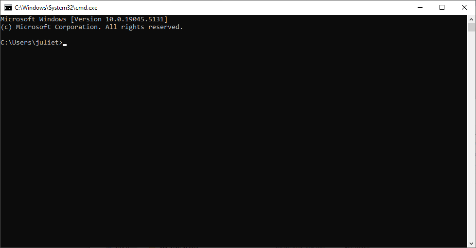
In the command prompt, paste the installer command you copied in the previous step. You should immediately see feedback that your computer is fetching Sireum Logika.
Once the installation is finished, open a file explorer and navigate to C:\Users\<yourAccountName>\Applications\Sireum\bin\win\vscodium. In that folder, you should see the application “CodeIVE.exe”. Double-click that application to run it (if you see a popup that asks if you want to allow access to your computer, go ahead and choose that you want to do so).
You may find it handy to pin the “CodeIVE.exe” application to your taskbar. You can do so by right-clicking the “CodeIVE.exe” file and selecting “Pin to taskbar”.
Installation and Running Sireum Logika - Mac
For Mac users, open a terminal window and paste the command you copied in the previous step. You should immediately see feedback that your computer is fetching Sireum Logika.
Once the installation is finished, go to the finder and search for “CodeIVE”. You should see the application “CodeIVE.exe” - if you run it, it will open Sireum Logika.
How to Start Homework Assignments
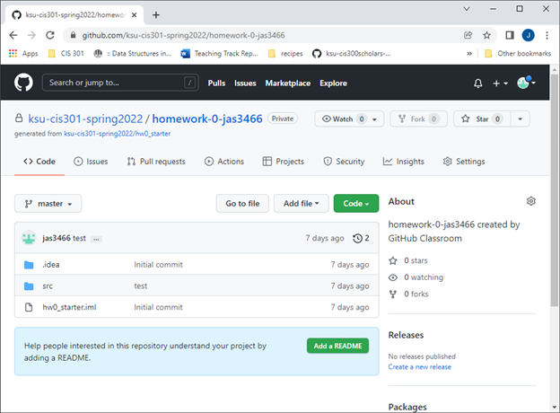
To start a homework assignment (or to clone any existing repository, including homework solutions and lecture examples), first:
- Click to “accept the assignment” from the link in Canvas (if you are cloning a homework assignment or solution).
- Go to the URL created for your assignment (or to the URL of the repository you want to clone).
- You should be looking at a website that looks something like this:
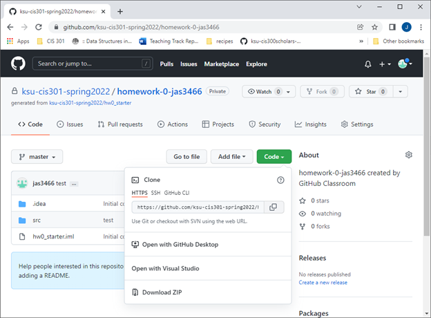
Get repo URL
Click the Green Code button, so that you see something like this:
Next, open Sireum VS Codium (by running the CodeIVE application). You should see:

Next, click the third icon in the column on the left side (the one that looks like a circuit and says “Source Control” when you hover over it). You should see:

Click Clone Repository. Now you should see something like:

Paste the URL you copied from GitHub in the textbox indicated above. Click “Clone from URL”.
You will then be prompted to choose a folder to clone your repository into. Navigate to a folder on your computer specifically for CIS 301 (create one if it doesn’t exist). Create a new empty folder within that CIS 301 folder to hold this new project. Select that new folder in the selection dialog, so that you now have something like this:

Click Select as Repository Destination. You should see a popup that asks if you want to open the cloned repository. Select “Open”. Next you should see something like:

If you see a popup in the bottom right that asks if you want to import a Sireum project, then click Yes.
Installing Sireum Fonts
When you have Sireum VS Codium open, click the gear icon in the lower-right corner. Click the option that says “Command Palette”:

Type “run” in the resulting textbox. Click the option that says: “Tasks: Run Task”.

Next, click the “sireum” folder:

Finally, click “sireum: –install-fonts”:

You might be asked for the installation location of Sireum at this point – if so, it is C:\Users\<yourAccountName>\Applications\Sireum for Windows and /Users/<yourAccountName>/Applications/Sireum for Mac. Windows users might need to type the location directly into the address bar if you can’t find the Applications folder in the file explorer.
If the new fonts (which show logic symbols instead of characters like & and |) don’t immediately appear, try restarting Sireum VS Codium.
Running Logika Checker
When you are ready to verify a Logika truth table or proof, click the gear icon in the lower-right corner and select “Command Palette”:
Type “run” in the resulting textbox. Click the option that says: “Tasks: Run Task”.
Next, click the “sireum logika” folder:

Finally, choose the option that says “sireum logika: verifier (file)”. You should see either a popup that says “Logika verified”, or you should see red error markings in your file indicating where the logic doesn’t hold up. You can hover over these red error markings to get popups with more information on the error.
As a shortcut to verify a proof or truth table, you can do: Ctrl-Shift-W on Windows or Command-Shift-W on Mac.
NOTE: You might be asked to choose the installation folder of Sireum the first time you run the Logika checker. If you are, the installation folder is C:\Users\<yourAccountName>\Applications\Sireum for Windows and /Users/<yourAccountName>/Applications/Sireum for Mac. Windows users might need to type the location directly into the address bar if you can’t find the Applications folder in the file explorer.
Committing and Pushing Changes
When you are finished working, commit and push your changes to GitHub. (I recommend doing this anytime you are at a stopping point, as well as when you are completely done.)
To do this, first save all your files (File-Save or Ctrl-S). Make sure none of the open file tabs have a solid circle next to the file name – this is an indication that they are unsaved. When everything is saved, open the integrated terminal in Code IVE by choosing View->Terminal. From there, type:
This will add all changes to the current commit. Then type:
git commit -m "descriptive message"
to create a local commit, where “descriptive message” is replaced with a message describing your changes (you DO need to include the quotations). Finally, push your local commit to your remote repository:
If you go to your GitHub repository URL and refresh the page, you should see the latest changes.
If you have any errors using a git command, refer to the next section (“git Install” for instructions on getting the command-line version of git).
Homework 0 will help you test the GitHub process.
Using Sireum in the Lab Classrooms
Sireum IVE (with Logika) is available in the CS computer lab classrooms (DUE 1114, 1116, and 1117). To find it, open a File Explorer, then open the C:\ drive. From there, navigate to “C:\Sireum\bin\win\vscodium” and run the “CodeIVE.exe” file. This will launch Sireum as usual.
If you want to complete your assignment using multiple computers, you can:
- Clone the repo using the process above (if it is your first time working on the current assignment on this computer)
- Commit/push your changes when you are ready to leave this computer
- Do Git->Pull to get your latest changes if you come back to a different computer
Remote Access
If you have any problems installing Sireum on your own computer, you can access it remotely from the CS department. See here for information on remote access. When you connect to the department Window’s server, you can follow the instructions above to find Sireum as you would on a lab computer.
git Install
Verify a git install
You will likely already have a command-line version of git installed on your machine. To check, open a folder in VS Code, display the integrated terminal, and type:
You should see a version number printing out. If you see that, git is already installed.
If you see an error that git is unrecognized, then you will need to install it. Go here to download and install the latest version.
Windows users may need to add the git.exe location to the system Path environment variables. Most likely, git.exe will be installed to C:\Program Files\Git\bin. Check this location, copy its address, and type “Environment variables” in the Windows search. Click “Environment Variables” and find “Path” under System variables. Click “Edit…”. Verify that C:\Program Files\Git\bin (or whatever your git location) is the last item listed. If it isn’t, add a new entry for C:\Program Files\Git\bin.
Subsections of Basics and Logic Puzzles
Basic Logical Reasoning
What is logical reasoning?
Logical reasoning is an analysis of an argument according to a set of rules. In this course, we will be learning several sets of rules for more formal analysis, but for now we will informally analyze English sentences and logic puzzles. This will help us practice the careful and rigorous thinking that we will need in formal proofs and in computer science in general.
Premises and conclusions
A premise is a piece of information that we are given in a logical argument. In our reasoning, we assume premises are true – even if they make no sense!
A conclusion in a logical argument is a statement whose validity we are checking. Sometimes we are given a conclusion, and we are trying to see whether that conclusion makes sense when we assume our premises are true. Other times, we are asked to come up with our own (valid) conclusion that we can deduce from our premises.
Example
Suppose we are given the following premises:
- Premise 1: If a person wears a red shirt, then they don’t like pizza.
- Premise 2: Fred is wearing a red shirt.
Given those pieces of information, can we conclude the following?
Fred doesn’t like pizza.
Yes! We take the premises at face value and assume them to be true (even though it is kind of ridiculous that shirt color has anything to do with a dislike of pizza). The first premise PROMISES that any time we have a person with a red shirt, then that person does not like pizza. Since Fred is such a person, we can conclude that Fred doesn’t like pizza.
Logical arguments with “OR”
Interpreting English sentences that use the word “or” can be tricky – the or can either be an inclusive or or an exclusive or. In programming, we are used to using an inclusive or – a statement like p || q is true as long as at least one of p or q is true, even if both are true. The only time a statement like p || q is false is if both p and q are false.
In English, however, the word “or” often implies an exclusive or. If a restaurant advertises that customers can choose “chips or fries” as the side for their meal, they are certainly not intending that a customer demand both sides.
However, since this course is focused on formal logic and analyzing computer programs and not so much on resolving language ambiguity, we will adopt the stance that the word “or” always means inclusive or unless otherwise specified.
Or example #1
With that in mind, suppose we have the following premises:
- I have a dog or I have a cat.
- I do not have a cat.
What can we conclude?
The only time an “or” statement true is when at least one of its parts is true. Since we already know that the right side of the or (“I have a cat”) is false, then we can conclude that the left side MUST be true. So we conclude:
I have a dog.
In general, if you have an or statement as a premise and you also know that one side of the or is NOT true, then you can always conclude that the other side of the or IS true.
Or example #2
Suppose we have the following premises:
- I have a bike or I have a car.
- I have a bike.
Can we conclude anything new?
First of all, I acknowledge that the most natural interpretation of the first premise is an exclusive or – that I have EITHER a bike OR a car, but not both. I think that is how most people would naturally interpret that sentence as well. However, in this course we will always consider “or” to be an inclusive or, unless we specifically use words like “but not both”.
With that in mind, the second premise is already sufficient to make the first premise true. Since I have a bike, the statement “I have a bike or I have a car” is already true, whether or not I have a car. Because of this, we can’t draw any further conclusions beyond our premises.
Or example 3
Suppose we have the following premises:
- I either have a bike or a car, but not both.
- I have a bike.
What can we conclude?
This is the sentence structure I will use if I mean an exclusive or – “either p or q but not both”.
In this setup, we CAN conclude that I do not have a car. This is because an exclusive or is FALSE when both sides are true, and I already know that one side is true (I have a bike). The only way for the first premise to be true is when I do not also have a car.
Logical arguments with if/then (aka implies, →)
Statements with of the form, if p, then q are making a promise – that if p is true, then they promise that q will also be true. We will later see this structure using the logical implies operator.
If/then example 1
Suppose we have the following premises:
- If it is raining, then I will get wet.
- It is raining.
What can I conclude?
The first premises PROMISES that if it is raining, then I will get wet. Since we assume this premise is true, then we must keep the promise. Since the second premise tells us that it IS raining, then we can conclude:
I will get wet.
If/then example 2
Suppose we have the following premises:
- If I don’t hear my alarm, then I will be late for class.
- I am late for class.
Can we conclude anything new?
The first premise promises that if I don’t hear my alarm, then I will be late for class. And if we knew that I didn’t hear my alarm, then we would be able to conclude that I will be late for class (in order to keep the promise).
However, we do NOT know that I don’t hear my alarm. All we are told is that I am late for class. I might be late for class for many reasons – maybe I got stuck in traffic, or my car broke down, or I got caught up playing a video game. We don’t have enough information to conclude WHY I’m late for class, and in fact we can’t conclude anything new at at all.
If/then example 3
Suppose we have the following premises:
- If I don’t hear my alarm, then I will be late for class.
- I’m not late for class.
What can we conclude?
This is a trickier example. We saw previously that the first premise promised that anytime I didn’t hear my alarm, then I would be late for class. But we can interpret this another way – since I’m NOT late for class, then I must have heard my alarm. After all, if I DIDN’T hear my alarm, then I would have been late. But I’m not late, so the opposite must be true. So we can conclude that:
I hear my alarm.
Reframing an if/then statement like that is called writing its contrapositive. Any time we have a statement of the form if p, then q then we can write the equivalent statement if not q, then not p.
Knights and Knaves
We will now move to solving several kinds of logic puzzles. While these puzzles aren’t strictly necessary to understand the remaining course content, they require the same rigorous analysis that we will use when doing more formal truth tables and proofs. Plus, they’re fun!
The puzzles in this section and the rest of this chapter are all either from or inspired by: What is the Name of This Book?, by Raymond Smullyan.
Island of Knights and Knaves
This section will involve knights and knaves puzzles, where we meet different inhabitants of the mythical island of Knights and Knaves. Each inhabitant of this island is either a knight or a knave.
Knights ALWAYS tell the truth, and knaves ALWAYS lie.
Example 1
Can any inhabitant of the island of Knights and Knaves say, “I’m a knave”?
-→ Click for solution
No! A knight couldn’t make that statement, as knights always tell the truth. And a knave couldn’t make that statement either, since it would be true – and knaves always lie.
Example 2
You see two inhabitants of the island of Knights and Knaves – Ava and Bob.
- Ava says that Bob is a knave.
- Bob says, “Neither Ava nor I are knaves.”
What types are Ava and Bob?
-→ Click for solution
Suppose Ava is a knight. Then her statement must be true, so Bob must be a knave. In this case, Bob’s statement would be a lie (since he is a knave), which is what we want.
Let’s make sure there aren’t any other answers that work.
Suppose instead that Ava is a knave. Then her statement must be a lie, so Bob must be a knight. This would mean that Bob’s statement should be true, but it’s not – Ava is a knave.
We can conclude that Ava is a knight and Bob is a knave.
Example 3
If you see an “or” statement in a knights and knaves puzzle, assume that it means an inclusive or. This will match the or logical operator in our later truth tables and proofs, and will also match the or operator in programmimg.
You see two different inhabitants – Eve and Fred.
- Eve says, “I am a knave or Fred is a knight.”
What types are Eve and Fred?
-→ Click for solution
Suppose first that Eve is a knight. Then her statement must be true. Since she isn’t a knave, the only way for her statement to be true is if Fred is a knight.
Let’s make sure there aren’t any other answers that work.
Suppose instead that Eve is a knave. Already we are in trouble – Eve’s statement is already true no matter what type Fred is. Since Eve would lie if she was a knave, we know she must not be knave.
We can conclude that Eve and Fred are both knights.
Example 4
You see three new inhabitants – Sarah, Bill, and Mae.
- Sarah tells you that only a knave would say that Bill is a knave.
- Bill claims that it’s false that Mae is a knave.
- Mae tells you, “Bill would tell you that I am a knave.”
What types are Sarah, Bill, and Mae?
-→ Click for solution
Before starting on this puzzle, it might help to rephrase Sarah’s and Bill’s statements. Sarah’s statement that only a knave would say that Bill is knave is really saying that it is FALSE that Bill is a knave (since knaves lie). Another way to say it’s false that Bill is a knave is to say that Bill is a knight. Similarly, we can rewrite Bill’s statemnet to say that Mae is a knight.
Now we have the following statements:
- Sarah tells you that Bill is a knight.
- Bill claims that Mae is a knight.
- Mae tells you, “Bill would tell you that I am a knave.”
Suppose Sarah is a knight. Then her statement is true, so Bill must also be a knight. This would mean Bill’s statement would also be true, so Mae is a knight as well. But Mae says that Bill would say she’s a knave, and that’s not true – Bill would truthfully say that Mae is a knight.
Suppose instead that Sarah is a knave. Then her statement is false, so Bill must be a knave. This would make Bill’s claim false as well, so Mae must be a knave. Mae knows that Bill would say she was a knight (since Bill is a knave, and would lie), and if Mae was a knave then she would indeed lie and say that Bill would say she was a knave.
We can conclude that all three are knaves.
Other Puzzles
We will look at a variety of other logic puzzles, each of which involve some statements being false and some statements being true.
Lion and Unicorn
The setup for a Lion and Unicorn puzzle can vary, but the idea is that both Lion and Unicorn have specific days that they tell only lies, and other specific days that they only tell the truth.
Here is one example:
Lion always lies on Mondays, Tuesdays, and Wednesdays.
Lion always tells the truth on other days.
Unicorn always lies on Thursdays, Fridays, and Saturdays, and always tells the truth on other days.
On Sunday, everyone tells the truth.
Lion says: “Yesterday was one of my lying days."
Unicorn says: “Yesterday was one of my lying days, too.”
What day is it?
-→ Click for solution
To solve this puzzle, we consider what Lion’s and Unicorn’s statements would mean on each different day of the week.
Suppose it is Sunday. Then Lion’s statement would be a lie (Lion does not lie on Saturday), and yet Lion is supposed to be telling the truth on Sunday.
Suppose it is Monday. Then both Lion’s and Unicorn’s statements would be lies, since they both told the truth yesterday (Sunday).
Suppose it is either Tuesday or Wednesday. Then Lion’s statement would be true – but Lion is supposed to lie on both Tuesday and Wednesday.
Suppose it is Thursday. Then Lion’s statement would be true (Wednesday was one of their lying days), which is good since Lion is supposed to be telling the truth on Thursdays. Similarly, Unicorn’s statement would be false (Unicorn does not lie on Thursdays), which works out since Unicorn DOES lie on Thursdays.
Suppose it is either Friday or Saturday. Then Lion’s statement would be a lie (Lion doesn’t lie on either Thursday or Friday), but Lion should be telling the truth on Friday and Saturday.
We can conclude that it must be Thursday.
Tweedledee and Tweedledum
The Tweedledee and Tweedledum puzzles originate from Through the Looking-glass and What Alice Found There, by Lewis Carroll. There are different versions of these puzzles as well, but all of them involve the identical twin creatures, Tweedledee and Tweedledum. Like with Lion and Unicorn, there are different days on which Tweedledee and Tweedledum either only lie or only tell the truth (and often one creature is lying while the other is telling the truth).
Example 1
Consider this puzzle:
Tweedledee and Tweedledum are identical. You know that one of them lies Mon/Tues/Wed,and that the other lies Thurs/Fri/Sat. (They tell the truth on non-lying days.)
You don’t know which is which.
You see both of them together.
The first one says: “I’m Tweedledum."
The second one says: “I’m Tweedledee.”
Which is which? What day is it?
-→ Click for solution
Answer: Since the two creatures gave different answers, we can conclude that they must both be lying or both telling the truth. (Otherwise, both creatures would give you the same name.) Sunday is the only such day.
Each is telling the truth, so the first twin is Tweedledum and the second is Tweedledee.
Example 2
Consider a second puzzle, with the same setup as to which days each twin lies and tells the truth.
You know that either Tweedledum or Tweedledee has lost a rattle. You find it, and want to return it to the correct one. You don’t know what day it is, but are sure that it isn’t Sunday (so one must be lying and one must be telling the truth).
The first one says: “Tweedledee owns the rattle.”
The second one says: “I’m Tweedledee ¬”
Who gets the rattle?
-→ Click for solution
To solve this puzzle, we can explore the possibilities for each twin lying or telling the truth.
Suppose the first twin is telling the truth. Since it isn’t Sunday, we know the second twin must be lying. If the second twin’s statement is a lie, then the second is Tweedledum. Since the first twin is telling the truth, then they are Tweedledee (and the owner of the rattle).
Suppose instead that the first twin is lying. Again, since it isn’t Sunday, we know the second twin must be telling the truth. This would make the second twin Tweedledee, and the first twin Tweedledum. It would also mean that TweedleDUM owns the rattle (since the first statement is a lie), which is the first twin.
We don’t have enough information to determine which twin is which, but it doesn’t matter – in both cases, the first twin is the owner of the rattle.
Portia’s Caskets
This type of puzzle originates from The Merchant of Venice, by William Shakespeare. In the play, Portia’s father devised riddles to test potential suitors for his daughter.
Here is one such puzzle:
There are three caskets – one gold, one silver, and one lead. One of the caskets contains a portrait (of Portia). Each casket has a message on it, and you know that at most one of the messages is true.
Gold casket message: “The portrait is in this casket.”
Silver casket message: “The portrait is not in this casket.”
Lead casket message: “The portrait is not in the gold casket.”
Where is the portrait?
-→ Click for solution
To solve this puzzle, we recognize that there are only three possibilities – the portrait must be in either the gold casket, the silver casket, or the lead casket. We consider the implications of each:
Suppose the portrait is in the gold casket. Then the messages on both the gold and silver caskets would be true. This isn’t possible, as we know that at most one of the messages is true.
Suppose instead that the portait is in the silver casket. Then the messages on the gold and silver caskets would be false, and the message on the lead casket would be true. Only one message is true, so this is a possibility.
Finally, suppose the portrait is in the lead casket. Then the messages on all three caskets would be true, so this isn’t possible.
We conclude that the portrait must be in the silver casket.
Subsections of Truth Tables
Operators and Circuits
In this chapter, we review basic notions about gates and learn the relationship between circuits and assignment-based computer programs. This sets the stage for analyzing modern programs.
Logical operators
There are four basic logic gates, with corresponding logical operators:
| Meaning | Logical Operator | Logic Gate |
|---|
| p AND q | p ∧ q | 
|
| p OR q | p ∨ q | 
|
| NOT p | ¬p | 
|
| p IMPLIES q | p → q | 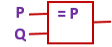
|
In the above drawings, the input wires are labelled with the names P and Q. The output that is computed is emitted from the rightmost wire which exits the gate. For these simple gates, it is possible to exhaustively test every permutation of potential inputs and summarize results in a table, called a truth table.
Let’s examine the AND gate. The AND gate emits a high voltage (1) exactly when high voltages are sensed at input wires P and Q; otherwise low voltage (0) is emitted. The gate’s physical behavior is summarized by in the following table:
AND: P Q |
-------------
     1 1 | 1
     1 0 | 0
     0 1 | 0
     0 0 | 0
Truth tables
For the remainder of this course, we will use T (read “true”) for 1 and F (read “false”) for 0. This is because we will examine applications that go far beyond circuit theory and base-two arithmetic. Here are the truth tables for the AND, OR, NOT and IMPLIES gates:
AND: P Q |
-------------
     T T | T
     T F | F
     F T | F
     F F | F


OR: P Q |
-------------
     T T | T
     T F | T
     F T | T
     F F | F


NOT: P |
-------------
     T | F
     F | T


IMPLIES: P Q |
-----------------
         T T | T
         T F | F
         F T | T
         F F | T
A few comments:
The OR gate is inclusive – as long as one of its inputs is true, then its output is true.
You might be confused by the IMPLIES gate. We’ll cover it in detail below.
In the next section, we will learn to write our truth tables in a slightly different format so they can be automatically checked by Sireum Logika.
Implies operator
The implies operator can be difficult to understand. It helps to think of it as a promise: we write P → Q, but we mean If P is true, then I promise that Q will also be true. If we BREAK our promise (i.e., if P is true but Q is false), then the output of an implies gate is false. In every other situation, the output of the implies gate is true.
As a reminder, here is the truth table for the implies operator, → :
P Q | P → Q
-----------------
T T |   T
T F |   F
F T |   T
F F |   T
It is likely clear why P → Q is true when both P and Q are true – in this situation, we have kept our promise.
It is also easy to understand why P → Q is false when P is true and Q is false. Here, we have broken our promise – P happened, but Q did not.
In the other two cases for P → Q we have that P is false (and Q is either true or false). Here, P → Q is true simply because we haven’t broken our promise. In these cases, the implication is said to be vacuously true because we have no evidence to prove that it is false.
Circuits
We can also compose the gates to define new operations.
For example, this circuit:
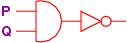
Written ¬(P ∧ Q), defines this computation of outputs:
P Q | ¬(P ∧ Q)
-----------------
T T | F
T F | T
F T | T
F F | T
We can work out the outputs in stages, like this:
We begin by writing the value of each set of inputs on the left, under their corresponding symbol on the right. Next we apply the operator (gate) with the highest precedence (covered in Operator Precedence in the next section). In our case the () make the AND ( ∧ ) symbol the highest.
A truth assignment is a unique permutation of the possible inputs for a system. For the ∧-gate, it is a 2-variable sequence. Considering the first row we see we have T ∧ T. Looking that up in the ∧-gate truth table we see the result is also “T”, and we record that under the ∧ symbol. We do the same thing all the other truth assignments.
After the initial transcribing of the truth values under their respective variables, we look up the truth-values in the gate tables, not the variables. Also observe that while ∧ is symmetric – i.e. T ∧ F and F ∧ T are both false – the IMPLIES gate is not.
Now we look up the value under the ∧ symbol in the ¬ gate table. In the first row we see that the truth assignment for the first row, “T”, is “F” and record it under the ¬ symbol. Do this for every row and we are done.
Truth Tables in Logika
Now that we’ve seen the four basic logic gates and truth tables, we can put them together to build bigger truth tables for longer logical formulae.
Operator precedence
Logical operators have a defined precedence (order of operations) just as arithmetic operators do. In arithmetic, parentheses have the highest precedence, followed by exponents, then multiplication and division, and finally addition and subtraction.
Here is the precedence of the logical operators, from most important (do first) to least important (do last):
- Parentheses
- Not operator,
¬ - And operator,
∧ - Or operator,
∨ - Implies operator,
→
For example, in the statement (p ∨ q) ∧ ¬p, we would evaluate the operators in the following order:
- The parentheses (which would resolve the
(p ∨ q) expression) - The not,
¬ - The and,
∧
Sometimes we have more than one of the same operator in a single statement. For example: p ∨ q ∨ r. Different operators have different rules for resolving multiple occurrences:
- Multiple parentheses - the innermost parentheses are resolved first, working from inside out.
- Multiple not (
¬ ) operators – the rightmost ¬ is resolved first, working from right to left. For example, ¬¬p is equivalent to ¬(¬p). - Multiple and (
∧ ) operators – the leftmost ∧ is resolved first, working from left to right. For example, p ∧ q ∧ r is equivalent to (p ∧ q) ∧ r. - Multiple or (
∨ ) operators – the leftmost ∨ is resolved first, working from left to right. For example, p ∨ q ∨ r is equivalent to (p ∨ q) ∨ r. - Multiple implies (
→ ) operators – the rightmost → is resolved first, working from right to left. For example, p → q → r is equivalent to p → (q → r).
Top-level operator
In a logical statement, the top-level operator is the operator that is applied last (after following the precedence rules above).
For example, in the statement:
p ∨ q → ¬p ∧ r
We would evaluate first the ¬, then the ∧, then the ∨, and lastly the →. Thus the → is the top-level operator.
Classifying truth tables
In our study of logic, it will be convenient to characterize logical formula with a description of their truth tables. We will classify each logical formula in one of three ways:
- Tautology - when all truth assignments for a logical formula are true
- Contradictory - when all truth assignments for a logical formula are false
- Contingent - when some truth assignments for a logical formula are true and some are false.
For example, p ∨ ¬ p is a tautology. Whether p is true or false, p ∨ ¬ p is always true.
On the other hand, p ∧ ¬ p is contradictory. Whether p is true or false, p ∧ ¬ p is always false.
Finally, something like p ∨ q is contingent. When p and q are both false, then p ∨ q is false. However, p ∨ q is true in every other case.
If all truth assignments for a logical formula are True, the formula is said to be a tautology.
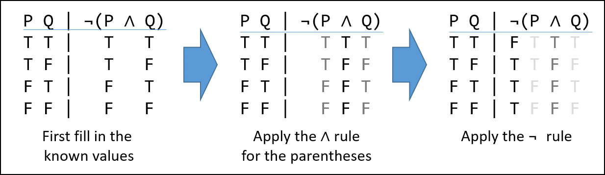
Logika syntax
From this point forward, the course will expect you to use Logika formatted truth tables. The Logika truth table for the formula ¬(p ∧ q) is:
      *
-----------------
p q # !(p & q)
-----------------
T T # F T T T
T F # T T F F
F T # T F F T
F F # T F F F
-----------------
Contingent
T: [T F] [F T] [F F]
F: [T T]
Logika truth tables have standard format (syntax) and semantic meanings. All elements of the truth table must be included to be considered correct.
The first line should have a single asterisk (*) over the top-level operator in the formula.
Next is a line of - (minus sign) characters, which must be at least as long as the third line to avoid getting errors.
The third line contains variables | formula. As Logika uses some capital letters as reserved words, you should use lower-case letters as variable names. Additionally, variables should be listed alphabetically.
The fourth line is another row of -, which is the same length as the second line.
Next come the truth assignments. Under the variables, list all possible combinations of T and F. Start with all T and progress linearly to all F. (T and F must be capitalized.)
After the Truth assignments is another row of -. Using each truth assignment, fill in truth assignments (T or F) under each operator in the formula in order of precedence (with the top-level operator applied last). Optionally, you can fill in the values for each variable under the forumla (as in the example above). However, it is only required that you fill in the truth assignments under each operator. Be careful to line up the truth assignments DIRECTLY below each operator, as Logika will reject truth tables that aren’t carefully lined up.
Under the truth assignments, put another line of - (minus sign) characters, which should be the same length as the second line.
Finally, classify the formula as either Tautology (if everything under the top-level operator is T), Contradictory (if everything under the top-level operator is F), or Contingent (if there is a mix of T and F under the top-level operator). If the formula is contingent, you must also list which truth assignments made the formula true (i.e., which truth assignments made the top-level operator T) and which truth assignments made the formula false. Follow the image above for the syntax of how to list the truth assignments for contingent examples.
Logical operators in Logika
You may notice that the example above appears to use the ! operator for NOT and the & operator for AND. However, what is shown above demonstrates what we TYPE into Logika, and not what is actually displayed. If we copy and paste the example into a new Logika file, it will look like:
      *
-----------------
p q # ¬(p ∧ q)
-----------------
T T # F T T T
T F # T T F F
F T # T F F T
F F # T F F F
-----------------
Contingent
T: [T F] [F T] [F F]
F: [T T]
Here is a summary of what keys to type in Logika for each traditional logical operator:
| Logical operator | What to TYPE in Logika | What you will SEE in Logika |
|---|
| NOT | ! | ¬ |
| OR | | | ∨ |
| AND | & | ∧ |
| IMPLIES | ->: | →: |
In the remainder of this book, my examples will be of what you will SEE in Logika.
Logika mishandling of implies operator
While the correct order of operations for logical operations is NOT, AND, OR, IMPLIES (from highest precedence to lowest precedence), the Logika tool does not handle the precedence of the implies operator correctly. The characters used for the implies operator in Logika are ->: – however, since Logika takes advantage of Scala’s operator precedence, this means that it interprets an implies operation as having the same (higher) precedence as a minus operation. In this class, we will always use parentheses to force the implies to have the correct precedence.
This incorrect precedence will only be present in our unit on truth tables – other proofs in Logika will use a different operator for implies (__>:) to avoid the issue of being interpreted as a minus operation. (We cannot use __>: in truth tables as the rendering makes the column alignment unclear.)
Example
Suppose we want to write a Logika truth table for:
First, we make sure we have a new file in Sireum with the .logika extension. Then, we construct this truth table shell:
                *
----------------------
p q r # (p ∧ q) →: ¬r
----------------------
T T T #
T T F #
T F T #
T F F #
F T T #
F T F #
F F T #
F F F #
----------------------
In the table above, we noticed that the → operator was the top-level operator according to our operator precedence rules.
Next, we fill in the output for the corresponding truth assignment under each operator, from highest precedence to lowest precedence. First, we evaluate the parentheses, which have the highest precedence. For example, we put a T under the ∧ in the first row, as p and q are both T in that row, and T ∧ T is T:
                *
----------------------
p q r # (p ∧ q) →: ¬r
----------------------
T T T #    T
T T F #    T
T F T #    F
T F F #    F
F T T #    F
F T F #    F
F F T #    F
F F F #    F
----------------------
In this example, we are only filling in under each operator (instead of also transcribing over each variable value), but either approach is acceptable.
Next, we fill in under the ¬ operator, which has the next-highest precedence:
                *
----------------------
p q r # (p ∧ q) →: ¬r
----------------------
T T T #    T       F
T T F #    T       T
T F T #    F       F
T F F #    F       T
F T T #    F       F
F T F #    F       T
F F T #    F       F
F F F #    F       T
----------------------
Then, we fill in under our top-level operator, the →. Notice that we must line up the T/F values under the → in the →: symbol. For example, we put a F under the →: on the first row, as (p ∧ q) is T there and ¬r is F, and we know that T→F is F because it describes a broken promise.
                *
----------------------
p q r # (p ∧ q) →: ¬r
----------------------
T T T #    T    F  F
T T F #    T    T  T
T F T #    F    T  F
T F F #    F    T  T
F T T #    F    T  F
F T F #    F    T  T
F F T #    F    T  F
F F F #    F    T  T
----------------------
Lastly, we examine the list of outputs under the top-level operator. We see that some truth assignments made the formula true, and that others (one) made the formula false. Thus, the formula is contingent. We label it as such, and list which truth assignments made the formula true and which made it false:
                *
----------------------
p q r # (p ∧ q) →: ¬r
----------------------
T T T #    T    F  F
T T F #    T    T  T
T F T #    F    T  F
T F F #    F    T  T
F T T #    F    T  F
F T F #    F    T  T
F F T #    F    T  F
F F F #    F    T  T
----------------------
Contingent
T: [T T F] [T F T] [T F F] [F T T] [F T F] [F F T] [F F F]
F: [T T T]
If you typed everything correctly and run a Logika check (Ctrl-Shift-W in Windows and Command-Shift-W on Mac), you should see a popup in Sireum logika that says: “Logika Verified” (yours will not have the purple checkmark, but will have the same text)
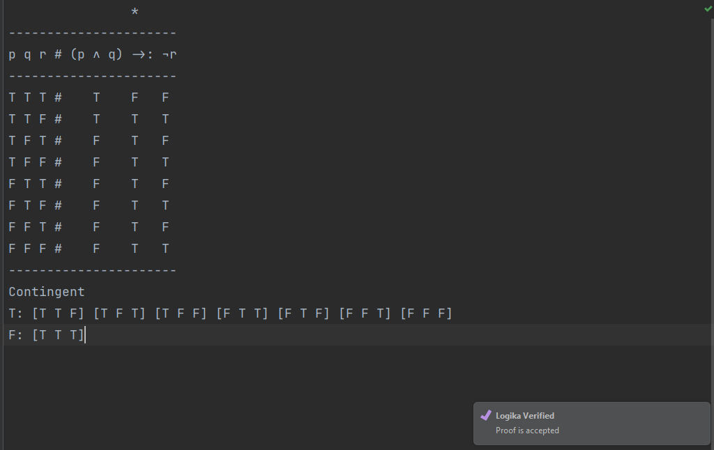
If you instead see red error markings, hover over them and read the explanations – it means there are errors in your truth table.
Satisfiability
We say that a logical statement is satisfiable when there exists at least one truth assignment that makes the overall statement true.
In our Logika truth tables, this corresponds to statements that are either contingent or a tautology. (Contradictory statements are NOT satisfiable.)
For example, consider the following truth tables:
          *
-----------------------
p q r # p →: q V ¬r ∧ p
-----------------------
T T T #   T    T F  F
T T F #   T    T T  T
T F T #   F    F F  F
T F F #   T    T T  T
F T T #   T    T F  F
F T F #   T    T T  F
F F T #   T    F F  F
F F F #   T    F T  F
------------------------
Contingent
T: [T T T] [T T F] [T F F] [F T T] [F T F] [F F T] [F F F]
F: [T F T]
And
      *
------------
p # p V ¬p
------------
T #   T F
F #   T T
-------------
Tautology
Both of these statements are satisfiable, as they have at least one (or more than one) truth assignment that makes the overall statement true.
Logical Equivalence
Two (or more) logical statements are said to be logically equivalent IFF (if and only if, ↔) they have the same truth value for every truth assignment; i.e., their truth tables evaluate exactly the same. (We sometimes refer to this as semantic equivalence.)
An example of logically equivalent statements are q ∧ p and p ∧ (q ∧ p):
         *
--------------
p q # (p ∧ q)
--------------
T T #    T
T F #    F
F T #    F
F F #    F
---------------
Contingent
T: [T T]
F: [F F] [F T] [T F]
         *
-------------------
p q #  p ∧ (q ∧ p)
-------------------
T T #    T    T
T F #    F    F
F T #    F    F
F F #    F    F
--------------------
Contingent
T : [T T]
F : [F F] [F T] [T F]
In these examples, notice that exactly the same set of truth assignments makes both statements true, and that exactly the same set of truth assignments makes both statements false.
Finding equivalent logical statements of fewer gates (states) is important to several fields. In computer science, fewer states can lead to less memory, fewer operations and smaller programs. In computer engineering, fewer gates means fewer circuits less power and less heat.
Common equivalences
We can similarly use truth tables to show the following common logical equivalences:
- Double negative:
¬ ¬ p and p - Contrapositive:
p → q and ¬ q → ¬ p - Expressing an implies using an OR:
p → q and ¬ p ∨ q - One of DeMorgan’s laws:
¬ (p ∧ q) and ( ¬ p ∨ ¬ q) - Another of DeMorgan’s laws:
¬ (p ∨ q) and ( ¬ p ∧ ¬ q)
Expressing additional operators
The bi-implication (↔) and exclusive or (⊕) operators are not directly used in this course. However, we can simulate both operators using a combination of ¬, ∧, ∨, and →:
p ↔ q, which means “p if and only if q”, can be expressed as (p → q) ∧ (q → p)p ⊕ q, which means “p exclusive or q”, can be expressed as (p ∨ q) ∧ ¬(p ∧ q)
Semantic Entailment
Definition
We say a set of premises, p1, p2, …, pn semantically entail a conclusion c, and we write:
if whenever we have a truth assignment that makes p1, p2, …, pn all true, then c is also true for that truth assignment.
(Note: we can use the ASCII replacement |= instead of the Unicode ⊨, if we want.)
Showing semantic entailment
Suppose we have premises p ∧ q and p → r. We want to see if these premises necessarily entail the conclusion r ∧ q.
First, we could make truth tables for each premise (being sure to list the variables p, q and r in each case, as that is the overall set of variables in the problem):
//truth table for premise, p ∧ q

          *
----------------------
p q r # p ∧ q
----------------------
T T T #   T
T T F #   T
T F T #   F
T F F #   F
F T T #   F
F T F #   F
F F T #   F
F F F #   F
----------------------
Contingent
T: [T T T] [T T F]
F: [T F T] [T F F] [F T T] [F T F] [F F T] [F F F]
//truth table for premise, p → r

          *
----------------------
p q r # p →: r
----------------------
T T T #   T
T T F #   F
T F T #   T
T F F #   F
F T T #   T
F T F #   T
F F T #   T
F F F #   T
----------------------
Contingent
T: [T T T] [T F T] [F T T] [F T F] [F F T] [F F F]
F: [T T F] [T F F]
Now, we notice that the truth assignment [T T T] is the only one that makes both premises true. Next, we make a truth table for our potential conclusion, r ∧ q (again, being sure to include all variables used in the problem):
//truth table for potential conclusion, r ∧ q
          *
----------------------
p q r # r ∧ q
----------------------
T T T #   T
T T F #   F
T F T #   F
T F F #   F
F T T #   T
F T F #   F
F F T #   F
F F F #   F
----------------------
Contingent
T: [T T T] [F T T]
F: [T T F] [T F T] [T F F] [F T F] [F F T] [F F F]
Here, we notice that the truth assignment [T T T] makes the conclusion true as well. So we see that whenever there is a truth assignment that makes all of our premises true, then that same truth assignment also makes our conclusion true.
Thus, p ∧ q and p → r semantically entail the conclusion r ∧ q, and we can write:
Semantic entailment with one truth table
The process of making separate truth tables for each premise and the conclusion, and then examining each one to see if any truth assignment that makes all the premises true also makes the conclusion true, is fairly tedious.
We are trying to show that IF each premise is true, THEN we promise the conclusion is true. This sounds exactly like an IMPLIES statement, and in fact that is what we can use to simplify our process. If we are trying to show that p1, p2, …, pn semantically entail a conclusion c (i.e., that p1, p2, ..., pn ⊨ c), then we can instead create ONE truth table for the statement:
(p1 ∧ p2 ∧ ... ∧ pn) → c
If this statement is a tautology (which would mean that anytime all the premises were true, then the conclusion was also true), then we would also have that the premises semantically entail the conclusion.
In our previous example, we create a truth table for the statement (p ∧ q) ∧ (p → r) → r ∧ q:
                           *
--------------------------------------
p q r # (p ∧ q) ∧ (p →: r) →: r ∧ q
--------------------------------------
T T T #    T    T    T     T    T
T T F #    T    F    F     T    F
T F T #    F    F    T     T    F
T F F #    F    F    F     T    F
F T T #    F    F    T     T    T
F T F #    F    F    T     T    F
F F T #    F    F    T     T    F
F F F #    F    F    T     T    F
---------------------------------------
Tautology
Then we see that it is indeed a tautology.
Subsections of Propositional Logic Translations
Propositional Atoms
Definition
A propositional atom is statement that is either true or false, and that contains no logical connectives (like and, or, not, if/then).
Examples of propositional atoms
For example, the following are propositional atoms:
- My shirt is red.
- It is sunny.
- Pigs can fly.
- I studied for the test.
Examples of what are NOT propositional atoms
Propositional atoms should not contain any logical connectives. If they did, this would mean we could have further subdivided the statement into multiple propositional atoms that could be joined with logical operators. For example, the following are NOT propositional atoms:
- It is not summer. (contains a not)
- Bob has brown hair and brown eyes. (contains an and)
- I walk to school unless it rains. (contains the word
unless, which has if…then information)
Propositional atoms also must be either true or false – they cannot be questions, commands, or sentence fragments. For example, the following are NOT propositional atoms:
- What time is it? (contains a question - not a true/false statement)
- Go to the front of the line. (contains a command - not a true/false statement)
- Fluffy cats (contains a sentence fragment - not a true/false statement)
Identifying propositional atoms
If we are given several sentences, we identify its propositional atoms by finding the key statements that can be either true or false. We further ensure that these statements do not contain any logical connectives (and, or, not, if/then information) - if they do, we break the statement down further. We then assign letters to each proposition.
For example, if we have the sentences:
My jacket is red and green. I only wear my jacket when it is snowing. It did not snow today.
Then we identify the following propositional atoms:
p: My jacket is red
q: My jacket is green
r: I wear my jacket
s: It is snowing
t: It snowed today
Notice that the first sentence, “My jacket is red and green”, contained the logical connective “and”. Thus, we broke that idea into its components, and got propositions p and q. The second sentence, “I only wear my jacket when it is snowing”, contained if/then information about when I would wear my jacket. We broke that sentence into two parts as well, and got propositions r and s. Finally, the last sentence, “It did not snow today”, contained the logical connective “not” – so we removed it and kept the remaining information for proposition t.
Each propositional atom is a true/false statement, just as is required.
In the next section, we will see how to complete our translation from English to propositional logic by connecting our propositional atoms with logical operators.
NOT, AND, OR Translations
Now that we have seen how to identify propositional atoms in English sentences, we will learn how to connect these propositions with logical operators in order to complete the process of translating from English to propositional logic.
NOT translations
When you see the word “not” and the prefixes “un-” and “ir-”, those should be replaced with a NOT operator.
Example 1
For example, if we have the sentence:
I am not going to work today.
Then we would first identify the propositional atom:
p: I am going to work today
and would then use a NOT operator to express the negation. Our full translation to propositional logic would be: ¬p
Example 2
As another example, suppose we have the sentence:
My sweater is irreplaceable.
We would identify the propositional atom:
p: My sweater is replaceable.
And again, our complete translation would be: ¬p
AND translations
When you see the words “and”, “but”, “however”, “moreover”, “nevertheless”, etc., then the English sentence is expressing a conjunction of ideas. When translating to propositional logic, all of these words should be replaced with a logical AND operator.
It might seem strange that the sentences “It is cold and it is sunny” and “It is cold but it is sunny” should be translated the same way – but really, both sentences are expressing two facts:
- It is cold
- It is sunny
Using “but” instead of “and” in English adds a subtle comparison of the first fact to the second fact, but such nuances are beyond the capabilities of propositional logic (and are somewhat ambiguous anyway).
Example 1
Suppose we want to translate the following sentence to propositional logic:
I like cake but I don't like cupcakes.
We would first identify two propositional atoms:
p: I like cake
q: I like cupcakes
We would then translate the clause “I don’t like cupcakes” to ¬q, and then would translate the connective “but” to a logical AND operator. We would finish with the following translation:
Example 2
Suppose we want to translate the following sentence to propositional logic:
The school doesn't have both a pool and a track.
We would first identify two propositional atoms:
p: The school has a pool
q: The school has a track
We would then see that we are really taking the sentence, “The school has a pool and a track” and negating it, which leaves us with the following translation:
OR translations
When you see the word “or” in a sentence, or some other clear disjunction of statements, then you will translate it to a logical OR operator. Because the word “or” in English can be ambiguous, We first need to determine whether the “or” is inclusive (in which case we would replace it with a regular OR operator) or exclusive (in which case we need to add a clause to explicitly express that both statements cannot be true).
As we saw in section 1.1, the word “or” in an English sentence is usually meant to be exclusive. However, because the logical OR is INclusive, and since the purpose of this class is not to have you wrestle with subtleties of the English language, then you can assume that an “or” in a sentence is inclusive unless clearly stated otherwise.
Inclusive OR statements
Suppose we want to translate the following sentence to propositional logic:
You watch a movie and/or eat a snack.
We would first identify two propositional atoms:
p: You watch a movie
q: You eat a snack
The “and/or” in our sentence makes it extremely clear that the intent is an inclusive or, since the sentence is true if you both watch a movie and eat a snack. This leaves us with the following translation:
Exclusive OR statements
In this class, if the meaning of “or” in a sentence is meant to be exclusive, then the sentence will clearly state that the two statements aren’t both true.
For example, suppose we want to translate the following sentence to propositional logic:
On Saturday, Jane goes for a run or plays basketball, but not both.
We would first identify two propositional atoms:
p: Jane goes for a run on Saturday
q: Jane plays basketball on Saturday
We then apply our equivalence for simulating an exclusive or operator, which we saw in section 2.4. This leaves us with the following translation:
Implies Translations
In this section, we will learn when to use an implies (→) operator when translating from English to propositional logic. In general, you will want to use an implies operator any time a sentence is making a promise – if one thing happens, then we promise that another thing will happen. The trick is to figure out the direction of the promise – promising that if p happens, then q will happen is subtly different from promising that if q happens, then p will happen.
Look for the words “if”, “only if”, “unless”, “except”, and “provided” as clues that the propositional logic translation will use an implies operator.
IF p THEN q statements
An “IF p THEN q” statement is promising that if p is true, then we can infer that q is also true. (It is making NO claims about what we can infer if we know q is true.)
For example, consider the following sentence:
If it is hot today, then I'll get ice cream.
We first identify the following propositional atoms:
p: It is hot today
q: I'll get ice cream
To determine the order of the implication, we think about what is being promised – if it is hot, then we can infer that ice cream will happen. But if we get ice cream, then we have no idea what the weather is like. It might be hot, but it might also be cold and I just decided to get ice cream anyway. Thus we finish with the following translation:
Alternatively, if we don’t get ice cream, we can be certain that it wasn’t hot – since we are promsied that if it is hot, then we will get ice cream. So an equivalent translation is:
(This form is called the contrapositive, which we learned about it in section 2.4). We’ll study it and other equivalent translations more in the next section.)
p IF q statements
A “p IF q” statement is promising that if q is true, then we can infer that p is also true. (It is making NO claims about what we can infer if we know p is true.) Equivalent ways of expressing the same promise are “p PROVIDED q” and “p WHEN q”.
For example, consider the following sentence:
You can login to a CS lab computer if you have a CS account.
We first identify the following propositional atoms:
p: You can login to a CS lab computer
q: You have a CS account
To determine the order of the implication, we think about what conditions need to be met in order for me to be promised that I can login. We see that if we have a CS account, then we are promised to be able to login. Thus we finish with the following translation:
In this example, if we knew we could login to a CS lab computer, we wouldn’t be certain that we had a CS account. There might be other reasons we can login – maybe you can use your eID account instead, for example.
Alternatively, if we can’t login, we can be certain that we don’t have a CS account. After all, we are guaranteed to be able to login if we do have a CS account. So another valid translation is:
p ONLY IF q
A “p ONLY IF q” statement is promising that the only time p happens is when q also happens. So if p does happen, it must be the case that q did too (since p can’t happen without q happening too).
For example, consider the following sentence:
Wilma eats cookies only if Evelyn makes them.
We first identify the following propositional atoms:
p: Wilma eats cookies
q: Evelyn makes cookies
What conditions need to be met for Wilma to eat cookies? If Wilma is eating cookies, Evelyn must have made cookies – after all, we know that Wilma only eats Evelyn’s cookies. Thus we finish with the following translation:
Equivalently, we are certain that if Evelyn DOESN’T make cookies, then Wilma won’t eat them – since she only eats Evelyn’s cookies. We can also write:
However, if we know that Evelyn makes cookies, we can’t be sure that Wilma will eat them. We know she won’t eat any other kind of cookie, but maybe Wilma is full today and won’t even eat Evelyn’s cookies…we can’t be sure.
p UNLESS q, p EXCEPT IF q
The statements “p UNLESS q” and “p EXCEPT IF q” are equivalent…and both can sometimes be ambiguous. For example, consider the following sentence:
I will bike to work unless it is raining.
We first identify the following propositional atoms:
p: I will bike to work
q: It is raining
Next, we consider what exactly is being promised:
- If it isn’t raining, will I bike to work? YES ¬ I promise to bike to work whenever it isn’t raining.
- If I don’t bike to work, is it raining? YES ¬ I always bike when it’s not raining, so if I don’t bike, it must be raining.
- If it’s raining, will I necessarily not bike to work? Well, maybe? Some people might interpret the sentence as saying I’ll get to work in another way if it’s raining, and others might think no promise has been made if it is raining.
- If I bike to work, is it necessarily not raining? Again, maybe? It’s not clear if I’m promising to only bike in non-rainy weather.
As we did with ambiguous OR statements, we will establish a rule in this class for intrepeting “unless” statements that will let us resolve ambiguity.
If you see the word unless when you are doing a translation, replace it with the words unless possibly if.
If we rephrase the sentence as:
I will bike to work *unless possibly if* it is raining.
We see that there is clearly NO promise about whether I will bike in the rain. I might, or I might not – but the only thing that I am promising is that I will bike if it is not raining, or that IF it’s not raining, THEN I will bike. With that in mind, we can complete our translation:
Equivalently, if we don’t bike, then we are certain that it must be raining – since we have promised to ride our bike every other time. We can also write:
Equivalent Translations
As we saw in section 2.4), two logical statements are said to be logically equivalent if and only if they have the same truth value for every truth assignment.
We can extend this idea to our propositional logic translations – two (English) statements are said to be equivalent iff they have the same underlying meaning, and iff their translations to propositional logic are logically equivalent.
Common equivalences, revisited
We previously identified the following common logical equivalences:
- Double negative:
¬ ¬ p and p - Contrapositive:
p → q and ¬ q → ¬ p - Expressing an implies using an OR:
p → q and ¬ p ∨ q - One of DeMorgan’s laws:
¬ (p ∧ q) and ( ¬ p ∨ ¬ q) - Another of DeMorgan’s laws:
¬ (p ∨ q) and ( ¬ p ∧ ¬ q)
Equivalence example 1
Suppose we have the following propositional atoms:
p: I get cold
q: It is summer
Consider the following three statements:
- I get cold except possibly if it is summer.
- If it’s not summer, then I get cold.
- I get cold or it is summer.
We translate each sentence to propositional logic:
I get cold except possibly if it is summer.
p → ¬q- Meaning: I promise that if I get cold, then it must not be summer…because I am always cold when it’s not summer.
If it’s not summer, then I get cold.
¬q → p- Meaning: I promise that anytime it isn’t summer, then I will get cold.
I get cold or it is summer.
p V q- Meaning: I’m either cold or it’s summer…because my being cold is true every time it isn’t summer.
As we can see, each of these statements is expressing the same idea.
Equivalence example 2
Suppose we have the following propositional atoms:
p: I eat chips
q: I eat fries
Consider the following two statements:
- I don’t eat both chips and fries.
- I don’t eat chips and/or I don’t eat fries.
We translate each sentence to propositional logic:
These statements are clearly expressing the same idea – if it’s not the case that I eat both, then it’s also true that there is at least one of the foods that I don’t eat. This is an application of one of DeMorgan’s laws: that ¬ (p ∧ q) is equivalent to ( ¬ p ∨ ¬ q).
If we were to create truth tables for both ¬(p ∧ q) and ¬p V ¬q, we would see that they are logically equivalent (that the same truth assignments make each statement true).
Equivalence example 3
Using the same propositional atoms as example 2, we consider two more statements:
- I don’t eat chips or fries.
- I don’t eat chips and I don’t eat fries.
We translate each sentence to propositional logic:
These propositions are clearly expressing the same idea – I have two foods (chips and fries), and I don’t eat either one. This demonstrates another of DeMorgan’s laws: that ¬ (p ∨ q) is equivalent to ( ¬ p ∧ ¬ q). If we were to create truth tables for each proposition, we would see that they are logically equivalent as well.
Knights and Knaves, revisited
Recall the Knights and Knaves puzzles from section 1.2. In addition to solving these puzzle by hand, we can devise a strategy to first translate a Knights and Knaves puzzle to propositional logic, and then solve the puzzle using a truth table.
Identifying propositional atoms
To translate a Knights and Knaves puzzle to propositional logic, we first create a propositional atom for each person that represented whether that person was a knight. For example, if our puzzle included the people “Adam”, “Bob”, and “Carly”, then we might create propositional atoms a, b, and c:
a: Adam is a knight
b: Bob is a knight
c: Carly is a knight
Translating statements
Once we have our propositional atoms, we can translate each statement in the puzzle to propositional logic. For each one, we want to capture that the statement is true IF AND ONLY IF the person speaking is a knight. (That way, the statement would be false whenever the person was not a knight – i.e., when they were a knave.) We recall that we can express if and only if using a conjunction of implications. So if we want to write p if and only if q, then we can say (p → q) ∧ (q → p).
As an example, suppose we have the following statement:
Adam says: Bob is a knight and Carly is a knave.
Adam’s statement should be true if and only if he is a knight, so we can translate it as follows:
(a → (b ∧ ¬c)) ∧ ((b ∧ ¬c) → a)
Which reads as:
If I am a knight, then Bob is a knight and Carly is a knave. Also, if Bob is a knight and Carly is a knave, then I am a knight.
We repeat this process for each statement in the puzzle. Finally, since we solve a Knights and Knaves puzzle by finding a truth assignment (i.e., assignment of who is a knight and who is a knave) that works for ALL statements, then we finish by AND-ing together our translations for each speaker. When we fill in the truth table for our final combined proposition, then a valid solution to the puzzle is any truth assignment that makes the overall proposition true. If it was a well-made puzzle, then there should only be one such truth assignment.
Full example
Suppose we meet two people on the Island of Knights and Knaves – Ava and Bob.
Ava says, "Bob and I are not the same".
Bob says, "Of Ava and I, exactly one is a knight."
We first create a propositional atom for each person:
a: Ava is a knight
b: Bob is a knight
Then, we translate each statement:
- Bob and I are not the same
- Translation:
(a → (a ∧ ¬b V ¬a ∧ b)) ∧ ((a ∧ ¬b V ¬a ∧ b) → a) - Meaning: If Ava is a knight, then either Ava is a knight and Bob is a knave, or Ava is a knave and Bob is a knight (so they aren’t the same type). Also, if Ava and Bob aren’t the same type, then Ava must be a knight (because her statement would be true).
- Bob says, “Of Ava and I, exactly one is a knight.
- Bob is really saying the same thing as Ava…if exactly one is a knight, then either Ava is a knight and Bob is a knave, or Ava is a knave and Bob is a knight.
- Translation:
(b → (a ∧ ¬b V ¬a ∧ b)) ∧ ((a ∧ ¬b V ¬a ∧ b) → b)
We combine our translations for Ava and Bob and end up with the following propositional logic statement:
(a → (a ∧ ¬b V ¬a ∧ b)) ∧ ((a ∧ ¬b V ¬a ∧ b) → a) ∧ (b → (a ∧ ¬b V ¬a ∧ b)) ∧ ((a ∧ ¬b V ¬a ∧ b) → b)`
We then complete the truth table for that proposition:
                                                                                  *
---------------------------------------------------------------------------------------------------------------
a b | (a →: (a ∧ ¬b V ¬a ∧ b)) ∧ ((a ∧ ¬b V ¬a ∧ b) →: a) ∧ (b →:(a ∧ ¬b V ¬a ∧ b)) ∧ ((a ∧ ¬b V ¬a ∧ b) →: b)
---------------------------------------------------------------------------------------------------------------
T T |    F     F F  F F  F     F     F F  F F  F    T     F    F    F  F F F  F     F     F  F F  F  F   T
T F |    T     T T  T F  F     T     T T  T F  F    T     T    T    T  T T F  F     F     T  T T  F  F   F
F T |    T     F F  T T  T     F     F F  T T  T    F     F    T    F  F T T  T     F     F  F T  T  T   T
F F |    T     F T  F T  F     T     F T  F T  F    T     T    T    F  T F T  F     T     F  T F  T  F   T
---------------------------------------------------------------------------------------------------------------
Contingent
T: [F F]
F: [T T] [T F] [F T]
And we see that there is only one truth assignment that satisfies the proposition – [F F], which corresponds to Ava being a knave and Bob being a knave.
Conclusion
As you can see, solving a Knights and Knaves problem by translating each statement to propositional logic is a tedious process. We ended up with a very involved final formula that made filling in the truth table somewhat arduous. Such problems are usually much simpler to solve by hand – but this process demonstrates that we can apply a systematic approach to solve Knights and Knaves problems with translations and truth tables.
Subsections of Propositional Logic Proofs
Introduction
While we can use truth tables to check whether a set of premises entail a conclusion, this requires testing all possible truth assignments – of which there are exponentially many. In this chapter, we will learn the process of natural deduction in propositional logic. This will allow us to start with a set of known facts (premises) and apply a series of rules to see if we can reach some goal conclusion. Essentially, we will be able to see whether a given conclusion necessarily follows from a set of premises.
We will use the Logika tool to check whether our proofs correctly follow our deduction rules. HOWEVER, these proofs can and do exist outside of Logika. Different settings use slightly different syntaxes for the deduction rules, but the rules and proof system are the same. We will merely use Logika to help check our work.
Sequents, premises, and conclusions
A sequent is a mathematical term for an assertion or an argument. We use the notation:
The p0, p1, …, pm are called premises and c is called the conclusion. The ⊢ is called the turnstile operator, and we read it as “prove”. The full sequent is read as:
Statements p0, p1, ..., pm PROVE c
A sequent is saying that if we accept statements p0, p1, …, pm as facts, then we guarantee that c is a fact as well.
For example, in the sequent:
The premises are: p → q and ¬q, and the conclusion is ¬p.
(Shortcut: we can use |- in place of the ⊢ turnstile operator.)
Sequent validity
A sequent is said to be valid if, for every truth assignment which make the premises true, then the conclusion is also true.
For example, consider the following sequent:
To check if this sequent is valid, we must find all truth assignments for which both premises are true, and then ensure that those truth assignments also make the conclusion true.
Sequent validity in Logika using truth tables
We can use a different kind of truth table to prove the validity of a sequent in Logika:
         *     *     *
---------------------------
p q # (p →: q, ¬q) ⊢ ¬p
---------------------------
T T #    T     F     F
T F #    F     T     F
F T #    T     F     T
F F #    T     T     T
---------------------------
Valid [F F]
Notice that instead of putting just one logical formula, we put the entire sequent – the premises are in a comma-separated list inside parentheses, then the turnstile operator (which we type using the keys |- in Logika), and then the conclusion. We mark the top-level operator of each premise and conclusion.
Examining each row in the above truth table, we see that only the truth assignment [F F] makes both premises (p → q and ¬q) true. We look right to see that the same truth assignment also makes the conclusion ( ¬p) true, which means that the sequent is valid.
Proving sequents using natural deduction
Now we will turn to the next section of the course – using natural deduction to similarly prove the validity of sequents. Instead of filling out truth tables (which becomes cumbersome very quickly), we will apply a series of deduction rules to allow us to conclude new claims from our premises. In turn, we can use our deduction rules on these new claims to conclude more and more, until (hopefully) we are able to claim our conclusion. If we can do that, then our sequent was valid.
Logika natural deduction proof syntax
We will use the following format in Logika to start a natural deduction proof for propositional logic. Each proof will be saved in a new file with a .sc (Scala) extension:
// #Sireum #Logika
//@Logika: --manual --background type

import org.sireum._
import org.sireum.justification._
import org.sireum.justification.natded.prop._

@pure def ProofName(variable1: B, variable2: B, ...): Unit = {
    Deduce(
        (comma-separated list of premises with variable1, variable2, ...)  ⊢  (conclusion)
            Proof(
                //the actual proof steps go here
            )
    )
}
Once we are inside the Proof element (where the above example says “the actual proof steps go here”), we complete a numbered series of steps. Each step includes a claim and corresponding justification, like this:
// #Sireum #Logika
//@Logika: --manual --background type

import org.sireum._
import org.sireum.justification._
import org.sireum.justification.natded.prop._

@pure def ProofName(variable1: B, variable2: B, ...): Unit = {
    Deduce(
        (comma-separated list of premises with variable1, variable2, ...)  ⊢  (conclusion)
            Proof(
                1 (     claim_a         )   by Justification_a,
                2 (     claim_b         )   by Justification_b,
                ...
                736 (   conclusion      )   by Justification_conc
            )
    )
}
Each claim is given a number, and these numbers are generally in order. However, the only rule is that claim numbers be unique (they may be out of order and/or non-consecutive). Once we have justified a claim in a proof, we will refer to it as a fact.
We will see more details of Logika proof syntax as we progress through chapter 4.
Premise justification
The most basic justification for a claim in a proof is “premise”. This justification is used when you pull in a premise from the sequent and introduce it into your proof. All, some or none of the premises can be introduced at any time in any order. Please note that only one premise may be entered per claim.
For example, we might bring in the premises from our sequent like this (the imports, proof function definition, deduce call, and formatter changes are omitted here for readability):
(p, q, ¬r)  ⊢  (p ∧ q)
    Proof(
        1 (     p               )   by Premise,
        2 (     q               )   by Premise,
        3 (     ¬r              )   by Premise,
        ...
    )
We could also bring in the same premise multiple times, if we wanted. We could also use non-sequential line numbers, as long as each line number was unique:
(p, q, ¬r)  ⊢  (p ∧ q)
    Proof(
        7 (     p           )   by Premise,
        10 (    q           )   by Premise,
        2 (     ¬r          )   by Premise,
        8 (     p           )   by Premise,
        ...
    )
We could only bring in some portion of our premises, if we wanted:
(p, q, ¬r)  ⊢  (p ∧ q)
    Proof(
        1 (     p           )   by Premise,
        ...
    )
But we can only list one premise in each claim. For example, the following is not allowed:
(p, q, ¬r)  ⊢  (p ∧ q)
    Proof(
        1 (     p, q, ¬r           )   by Premise,      //NO! Only one premise per line.
        ...
    )
Deduction rules
The logical operators (AND, OR, NOT, IMPLIES) are a kind of language for building propositions from basic, primitive propositional atoms. For this reason, we must have laws for constructing propositions and for disassembling them. These laws are called inference rules or deduction rules. A natural deduction system is a set of inference rules, such that for each logical operator, there is a rule for constructing a proposition with that operator (this is called an introduction rule) and there is a rule for disassembling a proposition with that operator (this is called an elimination rule).
For the sections that follow, we will see the introduction and elimination rules for each logical operator. We will then learn how to use these deduction rules to write a formal proof showing that a sequent is valid.
AND Rules
In this section, we will see the deduction rules for the AND operator.
AND introduction
Clearly, when both p and q are facts, then so is the proposition p ∧ q. This makes logical sense – if two propositions are independently true, then their conjunction (AND) must also be true. The AND introduction rule, AndI, formalizes this:
        P   Q
AndI :  ---------
        P ∧ Q
We will use the format above when introducing each of our natural deduction rules:
P and Q are not necessarily individual variables – they are placeholders for some propositional statement, which may itself involve several logical operators.- On the left side is the rule name (in this case,
AndI) - On the top of the right side we see what we already need to have established as facts in order to use this rule (in this case,
P and also Q ). These facts can appear anywhere in our scope of the proof, in whatever order. (For now, all previous lines in the proof will be within our scope, but this will change when we get to more complex rules that involve subproofs). - On the bottom of the right side, we see what we can claim by using that proof rule.
Here is a simple example of a proof that uses AndI. It proves that if propositional atoms p, q, and r are all true, then the proposition r ∧ (q ∧ p) is also true:
(p, q, r)  ⊢  (r ∧ (q ∧ p))
    Proof(
        1 (     p              )   by Premise,
        2 (     q              )   by Premise,
        3 (     r              )   by Premise,
        4 (     q ∧ p          )   by AndI(2, 1),
        5 (     r ∧ (q ∧ p)    )   by AndI(3, 4)
    )
You can read line 4 like this: “from the fact q stated on line 2 and the fact p stated on line 1, we deduce q ∧ p by applying the AndI rule”. Lines 4 and 5 construct new facts from the starting facts (premises) on lines 1-3.
Note that if I had instead tried:
(p, q, r)  ⊢  (r ∧ (q ∧ p))
    Proof(
        1 (     p              )   by Premise,
        2 (     q              )   by Premise,
        3 (     r              )   by Premise,
        4 (     q ∧ p          )   by AndI(1, 2),
        ...
    )
Then line 4 would not have been accepted. The line numbers cited after the AndI rule must match the order of the resulting AND statement. The left-hand side of our resulting AND statement must correspond to the first line number in AndI justification, and the right-hand side of our resulting AND statement must correspond to the second line number in the justification:
    ...
    4 (     p           )   by (some justification),
    5 (     q	        )   by (some justification),
    6 (     p ⋀ q       )   by AndI(4, 5),
    ...
    9 (     q ⋀ p       )   by AndI(5, 4),
    ...
AND elimination
The idea of the AND elimination rules is that if we have a proposition p ⋀ q as a fact, then we can separately claim both p and q as individual facts. After all, the only time p ⋀ q is true in a truth table is when both p and q are individually true. There are two AND elimination rules – AndE1 and AndE2. AndE1 allows us to claim that the left (first) side of an AND statement is individually true, and AndE2 allows us to do the same with the right (second) side. Here is the formalization of each rule:
        P ∧ Q                   P ∧ Q
AndE1 : ---------      AndE2 : ---------
          P                       Q
Here is a simple example showing the syntax of the AndE1 rule:
(p ∧ q)  ⊢  (p)
    Proof(
        1 (     p ∧ q          )   by Premise,
        2 (     p              )   by AndE1(1)
        ...
    )
We can read the justification AndE1(1) as: AND-elimination 1 from line 1, or “take the AND statement on line 1 and extract its first (left) side”.
Here is a simple example showing the syntax of the ∧e2 rule:
(p ∧ q)  ⊢  (q)
    Proof(
        1 (     p ∧ q          )   by Premise,
        2 (     q              )   by AndE2(1)
        ...
    )
We can read the justification AndE2(1) as: AND-elimination 2 from line 1, or “take the AND statement on line 1 and extract its second (right) side”.
Example 1
Suppose we want to prove the following sequent:
Whenever we approach a proof, a good first strategy is to see what we can extract from the premises. If we have a premise that is an AND statement, then we can use AndE1 and then AndE2 to extract both its left and right side as separate claims. So we start our proof like this:
(p ∧ (q ∧ r)) ⊢  (r ∧ p)
    Proof(
        1 (     p ∧ (q ∧ r)        )       by Premise,
        2 (     p                  )       by AndE1(1),
        3 (     q ∧ r              )       by AndE2(1),
        ...
    )
But now we have a new AND statement as a claim – q ∧ r. We can again use both AndE1 and AndE2 to extract each side separately:
(p ∧ (q ∧ r)) ⊢  (r ∧ p)
    Proof(
        1 (     p ∧ (q ∧ r)        )       by Premise,
        2 (     p                  )       by AndE1(1),
        3 (     q ∧ r              )       by AndE2(1),
        4 (     q                  )       by AndE1(3),
        5 (     r                  )       by AndE2(3),
        ...
    )
Now that we have done all we can with our premises and the resulting statements, we examine our conclusion. Whenever our conclusion is a conjunction (AND statement), we know that we must separately show both the left side and the right side of that conclusion. Then, we can use AndI to put those sides together into our goal AND statement.
In this example, we have already proved both sides of our goal AND statement – r (from line 5) and p (from line 2). All that remains is to use AndI to put them together:
(p ∧ (q ∧ r)) ⊢  (r ∧ p)
    Proof(
        1 (     p ∧ (q ∧ r)        )       by Premise,
        2 (     p                  )       by AndE1(1),
        3 (     q ∧ r              )       by AndE2(1),
        4 (     q                  )       by AndE1(3),
        5 (     r                  )       by AndE2(3),
        6 (     r ∧ p              )       by AndI(5, 2)
    )
Example 2
Suppose we want to prove the following sequent:
(p ∧ q ∧ r, a ∧ (t ∨ s)) ⊢ (q ∧ (t ∨ s))
We again try to use AND-elimination to extract what we can from our premises. We might try something like this:
(p ∧ q ∧ r, a ∧ (t ∨ s)) ⊢ (q ∧ (t ∨ s))
    Proof(
        1 (     p ∧ q ∧ r          )       by Premise,
        2 (     a ∧ (t ∨ s)        )       by Premise,
        3 (     p                  )       by AndE1(1),        //NO! Won't work.
        ...
    )
However, we get into trouble when we try to use AndE1 to extract the left side of the premise p ∧ q ∧ r. The problem has to do with operator precedence – we recall that ∧ operators are processed from left to right, which means that p ∧ q ∧ r is equivalent to (p ∧ q) ∧ r. By reminding ourselves of the “hidden parentheses”, we see that when we use AndE1 on the premise p ∧ q ∧ r, we extract p ∧ q. Similarly, AndE2 will extract r.
We try again to extract what we can from our premises:
(p ∧ q ∧ r, a ∧ (t ∨ s)) ⊢ (q ∧ (t ∨ s))
    Proof(
        1 (     p ∧ q ∧ r          )       by Premise,
        2 (     a ∧ (t ∨ s)        )       by Premise,
        3 (     p ∧ q              )       by AndE1(1),
        4 (     r                  )       by AndE2(1),
        5 (     a                  )       by AndE1(2),
        6 (     t ∨ s              )       by AndE2(2),
        ...
    )
As before, we look at our resulting claims – we see a p ∧ q, and we know that we can use AND elimination again to extract both sides. Now we have:
(p ∧ q ∧ r, a ∧ (t ∨ s)) ⊢ (q ∧ (t ∨ s))
    Proof(
        1 (     p ∧ q ∧ r          )       by Premise,
        2 (     a ∧ (t ∨ s)        )       by Premise,
        3 (     p ∧ q              )       by AndE1(1),
        4 (     r                  )       by AndE2(1),
        5 (     a                  )       by AndE1(2),
        6 (     t ∨ s              )       by AndE2(2),
        7 (     p                  )       by AndE1(3),
        8 (     q                  )       by AndE2(3),
        ...
    )
Now, we look at what we are trying to prove – q ∧ (t ∨ s). Since its top-level operator is the AND, we know that we must separately prove q and t ∨ s. Then, we can use AND introduction to put the two pieces together to match our conclusion. We see that we already have q on line 8 and t ∨ s on line 6, so we add our final line to finish the proof:
(p ∧ q ∧ r, a ∧ (t ∨ s)) ⊢ (q ∧ (t ∨ s))
    Proof(
        1 (     p ∧ q ∧ r          )       by Premise,
        2 (     a ∧ (t ∨ s)        )       by Premise,
        3 (     p ∧ q              )       by AndE1(1),
        4 (     r                  )       by AndE2(1),
        5 (     a                  )       by AndE1(2),
        6 (     t ∨ s              )       by AndE2(2),
        7 (     p                  )       by AndE1(3),
        8 (     q                  )       by AndE2(3),
        9 (     q ∧ (t ∨ s)        )       by AndI(8, 6)
    )
You might notice that lines 5 and 7 were not needed, as both p and a were not part of the conclusion. That’s true – we could have eliminated those steps. However, it’s a good idea to extract as much information as possible while you are getting used to doing these proofs – it doesn’t hurt to have extra claims, and you may find that you end up needing them.
OR Rules
In this section, we will see the deduction rules for the OR operator.
OR introduction
If we know that a proposition P is true, then it will also be the case that both P ∨ Q and Q ∨ P are also true. It doesn’t matter what Q is – it might even be something that is know to be false. Because P is true, it will make the overall OR statement true as well.
There are two OR introduction rules – OrI1 and OrI2. OrI1 allows us to claim an OR statement with some previous fact on the left (first) side, and OrI2 allows us to do the same with the right (second) side. Here is the formalization of each rule:
          P                   Q
OrI1 : --------    OrI2 :  --------
        P ∨ Q               P ∨ Q
Here is a simple example showing the syntax of the OrI1 rule:
(p) ⊢ (p ∨ q)
    Proof(
        1 (     p          )       by Premise,
        2 (     p ∨ q      )       by OrI1(1)
    )
We can read the justification OrI(1) as: OR introduction 1 from line 1, or “create a OR statement that puts the claim from line 1 on the first (left) side, and puts something new on the second side”.
Here is a simple example showing the syntax of the OrI2 rule:
(p) ⊢ (q ∨ p)
    Proof(
        1 (     p          )       by Premise,
        2 (     q ∨ p      )       by OrI2(1)
    )
We can read the justification OrI2(1) as: OR introduction 2 from line 1, or “create a OR statement that puts the claim from line 1 on the second (right) side, and puts something new on the first side”.
OR elimination
The OR elimination rule is used when we have an OR statement of the form P ∨ Q, and we wish to use it to extract new information. In real life, we call the rule “case analysis”. For example, say that you have either 12 quarters in your pocket or 30 dimes in your pocket. In either case, you can buy a $3.00 coffee. Why? You do a case analysis:
- In the case you have 12 quarters, that totals $3.00, and you can buy the coffee;
- In the case you have 30 dimes, that totals $3.00, and you can buy the coffee.
So, in both cases, you can buy the coffee.
We can formalize the idea behind the OR elimination rule as follows:
- In order for the OR statement
P ∨ Q to be true, at least one of P and Q must be individually true - If we are able to reach some conclusion
R if we assume P is true, and we are able to reach the SAME conclusion R if we assume Q is true… - …Then no matter what,
R will be true.
Subproofs
OR elimination will be our first proof rule that uses subproofs. Subproofs are tools for case analysis or what-if excursions, used to support justification for later claims. In propositional logic, they will always contain one assumption. This assumption is a proposition whose scope is limited to the subproof. The syntax of a subproof in Logika looks like this:
(premises) ⊢ (conclusion)
    Proof(
        ...
        5 (     fact_A             )   by Justification_A,
        ...
        17 SubProof(
            18 Assume(  fact_D  ),
            ...
            25 (    fact_G        )   by (some justification using claim 5)   //this is OK
            ...
        ),
        ...
        45 (    fact_R            )   by (some justification using claim 25)  //this is NOT OK
        ...
    )
Opening and closing parentheses, (...), that are attached to “Proof” and “SubProof” elements define the scope of claims. The SubProof elements are given a claim number when they are opened, but no justification. Closing parenthesis for ending proofs and subproofs are not given claim numbers. The use of parentheses in this manner is analogous to the use of curly brackets use to define scope in Java, C# and C.
In the example above, the subproof starting on line 17 creates an environment where fact_D is true. The justification used on claim number 25, which uses claim 15, is valid. The scope of claim 5 includes subproof 17.
However, the justification for line number 45 is invalid. Fact_G on line number 25 was proven true in an environment where fact_D is true (ie subproof 17). That environment ends (falls out of scope) when the closing parenthesis for the subproof is reached. This happens before line 45.
Only specific deduction rules allow you to close a scope and create a new claim based on that subproof in the enclosing (outer) scope. These rules always take a subproof (i.e “17”) as part of the justification.
Syntax
Here is the OR elimination rule:
                    SubProof(              SubProof(
                        Assume ( P ),           Assume ( Q ),
      P ∨ Q             ...                     ...
                        R                       R
                    ),                     ),
OrE : -----------------------------------------------------------
                         R
In order to use the OrE rule, we must have three things:
- An OR statement of the form
P ∨ Q - A subproof that begins by assuming the left side of the OR statement (
P) and ends with some claim R - A subproof that begins by assuming the right side of the OR statement (
Q) and ends with the same claim R
If we have all three parts, we can use the OrE and cite the OR statement and both subproofs to claim that R is true no matter what.
Here is a simple example showing the syntax of the OrE rule:
(p ∨ q) ⊢ (q ∨ p)
    Proof(
        1 (     p ∨ q          )           by Premise,

        2 SubProof(
            3 Assume (  p  ),
            4 (     q ∨ p      )           by OrI2(3)
        ),
        5 SubProof(
            6 Assume (  q   ),
            7 (     q ∨ p      )           by OrI1(6)
        ),
        8 (     q ∨ p          )           by OrE(1, 2, 5)
    )
Here, we have the OR statement p ∨ q. We then have two subproofs where we separately assume that the two sides or the OR are true. The first subproof on line 2 starts by assuming the left side of the OR, p. It then uses OR introduction to reach the goal conclusion, q ∨ p. After reaching our goal, we end the first subproof and immediately start a second subproof. In the second subproof, we assume that the the right side of our OR statement is true, q. We then use the other form of OR introduction to reach the SAME conclusion as we did in the first subproof – q ∨ p. We end the second subproof and can now use ∨e to state that our conclusion q ∨ p must be true no matter what. After all, we knew that at least one of p or q was true, and we were able to reach the conclusion q ∨ p in both cases.
When using the justification:
The first line number corresponds to our original OR statement (line 1 with p ∨ q for us), the second line number corresponds to the subproof where we assumed the first (left) side of that OR statement (line 2 for us, which starts the subproof where we assumed p), and the third line number corresponds to the subproof where we assumed the second (right) side of that OR statement (line 5 for us, which starts the subproof where we assumed q)
This proof shows that the OR operator is commutative.
Example 1
Suppose we want to prove the following sequent:
(p ∧ (q ∨ r)) ⊢ ((p ∧ q) ∨ (p ∧ r))
As we have done before, we start by extracting whatever we can from our premises:
(p ∧ (q ∨ r)) ⊢ ((p ∧ q) ∨ (p ∧ r))
    Proof(
        1 (     p ∧ (q ∨ r)        )   by Premise,
        2 (     p                  )   by AndE1(1),
        3 (     q ∨ r              )   by AndE2(1),
        ...
    )
Next, we look at what we are trying to prove, and see that its top-level operator is an OR. If we already had either side of our goal OR statement (i.e., either p ∧ q or p ∧ r), then we could use AndI to create the desired proposition. This isn’t the case for us, though, so we need to use a different strategy.
The next consideration when we want to prove an OR statement is whether we have another OR statement, either as a premise or a fact we have already established. If we do, then we can attempt to use OR elimination with that OR statement to build our goal conclusion ((p ∧ q) ∨ (p ∧ r)). We have the OR statement q ∨ r available, so we’ll try to use OR elimination – we’ll have a subproof where we assume q and try to reach (p ∧ q) ∨ (p ∧ r), and then a subproof where we assume r and try to reach (p ∧ q) ∨ (p ∧ r):
(p ∧ (q ∨ r)) ⊢ ((p ∧ q) ∨ (p ∧ r))
    Proof(
        1 (     p ∧ (q ∨ r)            )   by Premise,
        2 (     p                      )   by AndE1(1),
        3 (     q ∨ r                  )   by AndE2(1),

        4 SubProof(
            5 Assume(  q  ),
            6 (     p ∧ q              )   by AndI(2,5),
            7 (     (p ∧ q) ∨ (p ∧ r)  )   by OrI1(6)
        ),
        8 SubProof(
            9 Assume(  r  ),
            10 (    p ∧ r             )   by AndI(2,9),
            11 (    (p ∧ q) ∨ (p ∧ r) )   by OrI2(10)
        ),
        12 (  (p ∧ q) ∨ (p ∧ r)     )   by OrE(3, 4, 8)
    )
We can make our final claim:
12 ( (p ∧ q) ∨ (p ∧ r) ) by OrE(3, 4, 8)
Because we had an OR statement on line 3 (q ∨ r), assumed the left side of that OR (q) in subproof 4 and reached the conclusion of (p ∧ q) ∨ (p ∧ r), and then assumed the right side of our OR (r) in subproof 8 and reached the SAME conclusion of (p ∧ q) ∨ (p ∧ r).
Example 2
Suppose we want to prove the following sequent:
((p ∨ q) ∧ (p ∨ r)) ⊢ (p ∨ (q ∧ r))
Note that this is the same as the previous example, but the premises are switched with the conclusion. If we prove this direction too, we will have shown that (p ∨ q) ∧ (p ∨ r) is equivalent to p ∨ (q ∧ r). We’ll learn more about this process in section 4.8.
We start by pulling in our premises and extracting whatever information we can:
((p ∨ q) ∧ (p ∨ r)) ⊢ (p ∨ (q ∧ r))
    Proof(
        1 (     (p ∨ q) ∧ (p ∨ r)      )   by Premise,
        2 (     p ∨ q                  )   by AndE1(1),
        3 (     p ∨ r                  )   by AndE2(1),
        ...
    )
We see that the top-level operator of our conclusion (p ∨ (q ∧ r)) is an OR, so we apply the same strategy we did in the previous example – we see if we have an OR statement already available as a claim, and then try to use OR elimination on it to build to our conclusion in both subproofs. In this case, though, we have TWO or statements – p ∨ q and p ∨ r. We will see that it doesn’t matter which of these we choose, so let’s pick the first one – p ∨ q:
((p ∨ q) ∧ (p ∨ r)) ⊢ (p ∨ (q ∧ r))
    Proof(
        1 (     (p ∨ q) ∧ (p ∨ r)       )   by Premise,
        2 (     p ∨ q                   )   by AndE1(1),
        3 (     p ∨ r                   )   by AndE2(1),

        4 SubProof(
            5 Assume(  p  ),
            6 (     p ∨ (q ∧ r)         )   by OrI1(5)
        )
        7 SubProof(
            8 Assume(   q               ),

            //what do we do now?
        )
        ...
    )
We are able to finish the first subproof, but it’s not clear what to do in the second subproof. We assume q, and know we have the goal of reaching the same conclusion as we did in the first subproof, p ∨ (q ∧ r)…but we don’t have enough information yet to get there. The only piece of information that we haven’t used that might help us is our second OR statement – p ∨ r. We are already inside a subproof, but we can still nest other subproofs – just as we can nest conditional statements in computer programs.
We start on a nested OR elimination approach with p ∨ r:
((p ∨ q) ∧ (p ∨ r)) ⊢ (p ∨ (q ∧ r))
    Proof(
        1 (     (p ∨ q) ∧ (p ∨ r)       )   by Premise,
        2 (     p ∨ q                   )   by AndE1(1),
        3 (     p ∨ r                   )   by AndE2(1),

        4 SubProof(
            5 Assume(  p  ),
            6 (     p ∨ (q ∧ r)         )   by OrI1(5)
        ),
        7 SubProof(
            8 Assume(  q  ),

            //start OR elimination with p ∨ r
            9 SubProof(
                10 Assume(  p  ),
                11 (    p ∨ (q ∧ r)     )   by OrI1(10)
            ),
            12 SubProof(
                13 Assume(  r  ),
                14 (    q ∧ r           )   by AndI(8, 13),
                15 (    p ∨ (q ∧ r)     )   by OrI2(14)
            ),
            16 (    p ∨ (q ∧ r)         )   by OrE(3, 9, 12)
        ),
        17 (    p ∨ (q ∧ r)             )   by OrE(2, 4, 7)
    )
Note that we use the ∨e rule twice – on line 16 to tie together subproofs 9 and 12 (where we processed the OR statement p ∨ r), and on line 17 to tie together subproofs 4 and 7 (where we processed the OR statement p ∨ q).
When we first started this problem, we mentioned that it didn’t matter which OR statement we chose to work with – p ∨ q or p ∨ r. Indeed, we could have chosen p ∨ r instead – but we would end up nesting another OR elimination for p ∨ q:
((p ∨ q) ∧ (p ∨ r)) ⊢ (p ∨ (q ∧ r))
    Proof(
        1 (     (p ∨ q) ∧ (p ∨ r)      )   by Premise,
        2 (     p ∨ q                  )   by AndE1(1),
        3 (     p ∨ r                  )   by AndE2(1),

        //OR elimination for p ∨ r
        4 SubProof(
            5 Assume(  p  ),
            6 (     p ∨ (q ∧ r)        )   by OrI1(5)
        ),
        7 SubProof(
            8 Assume(  r  ),

            //start OR elimination with p ∨ q
            9 SubProof(
                10 Assume(  p  ),
                11 (    p ∨ (q ∧ r)   )   by OrI1(10)
            ),
            12 SubProof(
                13 Assume(  q  ),
                14 (    q ∧ r         )   by AndI(13, 8),
                15 (    p ∨ (q ∧ r)   )   by OrI2(14)
            ),
            16 (    p ∨ (q ∧ r)       )   by OrE(2, 9, 12)
        ),
        17 (    p ∨ (q ∧ r)           )   by OrE(3, 4, 7)
    )
Implies Rules
In this section, we will see the deduction rules for the implies operator.
Note that in our Logika proofs, the implies operator is typed as __>: but is rendered as →.
Implies elimination
Remember that → is a kind of logical “if-then”. Here, we understand p → q to mean that p holds knowledge sufficient to deduce q – so, whenever p is proved to be a fact, then p → q enables q to be proved a fact, too. This is the implies elimination rule, ImplyE, and we can formalize it like this:
            P → Q    P
 ImplyE :  ------------
                Q
Here is a simple example of a proof that shows the syntax of the ImplyE rule:
(a, a → b) ⊢ (b)
    Proof(
        1 (     a          )   by Premise,
        2 (     a → b      )   by Premise,
        3 (     b          )   by ImplyE(2, 1)
    )
Note that when we use ImplyE, we first list the line number of the implies statement, and then list the line number that contains the left side of that implies statement. The ImplyE allows us to claim the right side of that implies statement.
Implies introduction
The idea behind the next deduction rule, implies introduction, is that we would be introducing a new implies statement of the form P → Q. In order to do this, we must be able to show our logical “if-then” – that IF P exists, THEN we promise that Q will also exist. We do this by way of a subproof where we assume P. If we can reach Q by the end of that subproof, we will have shown that anytime P is true, then Q is also true. We will be able to close the subproof by introducing P → Q with the ImplyI rule. We can formalize the rule like this:
           SubProof(
              Assume(  P  ),
              ...
              Q
           ),
ImplyI : --------------
              P → Q
Here is a simple example of a proof that shows the syntax of the ImplyI rule:
(a → b, b → c) ⊢ (a → c)
    Proof(
        1 (     a → b           )   by Premise,
        2 (     b → c           )   by Premise,
        3 SubProof(
            //we want to prove a → c, so we start by assuming a

            4 Assume(  a  ),
            5 (     b           )   by ImplyE(1, 4),
            6 (     c           )   by ImplyE(2, 5)

            //...and try to end with c
        ),
        //then we can conclude that anytime a is true, then c is also true

        7 (     a → c           )   by ImplyI(3)
    )
Note that when we use ImplyI, we list the line number of the subproof we just finished. We must have started that subproof by assuming the left side of the implies statement we are introducing, and ended that subproof with the right side of the implies statement we are introducing.
Example 1
Suppose we want to prove the following sequent:
(p → (q → r)) ⊢ ((q ∧ p) → r)
We start by listing our premise:
(p → (q → r)) ⊢ ((q ∧ p) → r)
    Proof(
        1 (     p → (q → r)        )   by Premise,
        ...
    )
We can’t extract any information from the premise, so we shift to examining our conclusion. The top-level operator of our conclusion is an implies statement, so this tells us that we will need to use the ImplyI rule. We want to prove (q ∧ p) → r, so we need to show that whenever q ∧ p is true, then r is also true. We open a subproof and assume the left side of our goal implies statement (q ∧ p). If we can reach r by the end of the subproof, then we can use ImplyI to conclude (q ∧ p) → r:
(p → (q → r)) ⊢ ((q ∧ p) → r)
    Proof(
        1 (     p → (q → r)        )   by Premise,

        2 SubProof(
            3 Assume(  q ∧ p  ),

            //goal: get to r
        ),
        //use ImplyI to conclude (q ∧ p) → r
    )
Now we can complete the proof:
(p → (q → r)) ⊢ ((q ∧ p) → r)
    Proof(
        1 (     p → (q → r)        )   by Premise,

        2 SubProof(
            3 Assume(  q ∧ p  ),
            4 (     q              )   by AndE1(3),
            5 (     p              )   by AndE2(3),
            6 (     q → r          )   by ImplyE(1, 5),
            7 (     r              )   by ImplyE(6, 4)

            //goal: get to r
        ),

        //use ImplyI to conclude (q ∧ p) → r
        8 (     (q ∧ p) → r        )   by ImplyI(2)
    )
Example 2
Suppose we want to prove the following sequent:
(p → (q → r) ⊢ (p → q) → (p → r))
We see that we will have no information to extract from the premises. The top-level operator is an implies statement, so we start a subproof to introduce that implies statement. In our subproof, we will assume the left side of our goal implies statement (p → q) and will try to reach the right side of our goal (p → r):
(p → (q → r) ⊢ (p → q) → (p → r))
    Proof(
        1 (     p → (q → r)            )   by Premise,

        2 SubProof(
            3 Assume(  p → q  ),

            //goal: get to p → r
        ),
        //use ImplyI to conclude (p → q) → (p → r)
    )
We can see that our goal is to reach p → r in our subproof – so we see that we need to introduce another implies statement. This tells us that we need to nest another subproof – in this one, we’ll assume the left side of our current goal implies statement (p), and then try to reach the right side of that current goal (r). Then, we’d be able to finish that inner subproof by using ImplyI to conclude p → r:
(p → (q → r) ⊢ (p → q) → (p → r))
    Proof(
        1 (     p → (q → r)            )   by Premise,

        2 SubProof(
            3 Assume(  p → q  ),

            4 SubProof(
                5 Assume(  p  ),

                //goal: get to r
            ),
            //use ImplyI to conclude p → r

            //goal: get to p → r
        ),
        //use ImplyI to conclude (p → q) → (p → r)
    )
Now we can complete the proof:
(p → (q → r) ⊢ (p → q) → (p → r))
    Proof(
        1 (     p → (q → r)             )   by Premise,

        2 SubProof(
            3 Assume(  p → q  ),

            4 SubProof(
                5 Assume(  p  ),
                6 (     q               )   by ImplyE(3, 5),
                7 (     q → r           )   by ImplyE(1, 5),
                8 (     r               )   by ImplyE(7, 6)

                //goal: get to r
            ),
            //use ImplyI to conclude p → r

            9 (     p → r               )   by ImplyI(4)

            //goal: get to p → r
        ),
        //use ImplyI to conclude (p → q) → (p → r)

        10 (    (p → q) → (p → r)       )   by ImplyI(2)
    )
Example 3
Here is one more example, where we see we can nest an ImplyI subproof and a OrE subproof:
(p → r, q → r) ⊢ ((p ∨ q) → r)
    Proof(
        1 (     p → r              )   by Premise,
        2 (     q → r              )   by Premise,
        3 SubProof(
            //assume p ∨ q, try to get to r

            4 Assume(  p ∨ q  ),

            //nested subproof for OR elimination on p ∨ q
            //try to get to r in both cases

            5 SubProof(
                6 Assume(  p  ),
                7 (     r          )   by ImplyE(1, 6)
            ),
            8 SubProof(
                9 Assume(  q  ),
                10 (    r          )   by ImplyE(2, 9)
            ),
            11 (    r              )   by OrE(4, 5, 8)

            //goal: get to r
        ),

        //use ImplyI to conclude (p ∨ q) → r
        12 (    (p ∨ q) → r        )   by ImplyI(3)
    )
Negation Rules
In this section, we will see the deduction rules for the NOT operator. In this section, we will introduce the notion of a contradiction, which occurs when, for some proposition P, we have proved both the facts P and ¬ P. This indicates that we are in an impossible situation, and often means that we have made a bad previous assumption. In Logika, we use an F (“false”) as a claim to indiciate that we’ve reached a contradiction. In other texts, you sometime see the symbol ⊥ (which means “bottom operator”) for a contradiction.
Negation elimination
The negation elimination rule allows you to claim that you have reached a contradiction. We can formalize the rule like this:
        P   ¬P
NegE : -----------
           F
Here is a simple example of a proof that shows the syntax of the `NegE rule:
(q, ¬q) ⊢ (F)
    Proof(
        1 (     q       )   by Premise,
        2 (     ¬q      )   by Premise,
        3 (     F       )   by NegE(1, 2)
    )
We use the NegE rule when we have facts for both P and ¬P for some proposition P. When we use the justification, we first list the line number of the claim for P (line 1, in our case) and then the line number of the claim for ¬P (line 2, in our case).
Sometimes, the proposition P itself has a NOT operator. Consider this example:
(¬q, ¬¬q) ⊢ (F)
    Proof(
        1 (     ¬q      )   by Premise,
        2 (     ¬¬q     )   by Premise,
        3 (     F       )   by NegE(1, 2)
    )
Here, our proposition P is the claim ¬q, and our proposition that is of the form ¬P is the claim ¬¬q.
Negation introduction
The negation introduction rule allows us to introduce a NOT operation. If assuming some proposition P leads to a contradiction, then we must have made a bad assumption – P must NOT be true after all. We can then introduce the fact ¬P. We can formalize the negation introduction rule like this:
        SubProof(
            Assume ( P ),
            ...
            F
        ),
NegI : --------------
           ¬P
Here is a simple example of a proof that shows the syntax of the NegI rule:
(p,  q → ¬p)  ⊢  (¬q)
    Proof(
        1 (     p           )       by Premise,
        2 (     q → ¬p      )       by Premise,

        3 SubProof(
            4 Assume (  q  ) ,
            5 (     ¬p      )       by ImplyE(2, 4),
            6 (     F       )       by NegE(1, 5)
        ),
        7 (     ¬q          )       by NegI(3)
    )
Note that the negation introduction rule involves a subproof – if we wish to prove ¬P for some proposition P, then we start a subproof where we assume P. If we are able to reach a contradiciton on the last line of that subproof, then we can use the NegI rule after the subproof ends to claim that our assumption was bad and that it is actually ¬P that is true. When we use ¬i as a justification, we list the line number corresponding to this subproof.
Bottom elimination
There is a special law for reasoning forwards from an impossible situation — the ⊥e law — which says, in the case of a contradiction, everything becomes a fact. (That is, “if False is a fact, so is everything else ¬”.) This rule is called “bottom elimination”, and is written as BottomE. Here is a formalization of the rule:
              F
BottomE :  ------  for any proposition, Q, at all
              Q
Here is a simple example of a proof that shows the syntax of the BottomE rule:
(p, ¬p)  ⊢ (q)
Proof(
    1 (     p       )       by Premise,
    2 (     ¬p      )       by Premise,
    3 (     F       )       by NegE(1, 2),
    4 (     q       )       by BottomE(3)
)
Note that when we use BottomE as the justification, we list the line number of where we reached a contradiction (F).
The bottom elimination rule works well with case analysis, where we discover that one case is impossible. Here is a classic example:
(p ∨ q, ¬p) ⊢ (q)
    Proof(
        1 (     p ∨ q       )   by Premise,
        2 (     ¬p          )   by Premise,

        3 SubProof(
            4 Assume(  p  ),
            5 (     F       )   by NegE(4, 2),
            6 (     q       )   by BottomE(5)
        ),
        7 SubProof(
            8 Assume(  q  )
        ),
        9 (     q           )   by OrE(1, 3, 7)
    )
Considering the premise, p ∨ q, we analyze our two cases by starting OR elimination. The first case, where p holds true, is impossible, because it causes a contradiction. The BottomE-rule lets us gracefully prove q in this “impossible case”. (You can read lines 4-6 as saying, “in the case when p might hold true, there is a contradiction, and in such an impossible situation, we can deduce whatever we like, so we deduce q to finish this impossible case”.)
The second case, that q holds true, is the only realistic case, and it immediately yields the conclusion. The proof finishes the two-case analysis with the OrE rule.
Proof by contradiction
The proof by contraction rule, PbC, says that when assuming ¬P leads to a contradiction for some proposition P, then we made a bad assumption and thus P must be true. It is very similar to the NegI rule, except PbC has us assuming ¬P and eventually concluding P, while the NegI rule has us assuming P and eventually concluding ¬P.
Here is a formalization of PbC:
        SubProof(
             Assume( ¬P ),
             ...
             F
        ),
PbC:   --------------------
               P
And here is an example that demonstrates the syntax of the rule:
(¬¬p) ⊢ (p)
Proof(
    1 (     ¬¬p         )   by Premise,

    2 SubProof(
        3 Assume (  ¬p  ),
        4 (     F       )   by NegE(3, 1)
    ),
    5 (     p           )   by PbC(2)
)
When we use the PbC rule as a justification for a claim P, we cite the line number of the subproof where we assumed ¬P and ended in a contradiction.
Example 1
Suppose we want to prove the following sequent:
We start by listing our premise, and extracting the two sides of the AND statement:
(¬p ∧ ¬q) ⊢ (¬(p ∨ q))
    Proof(
        1 (     ¬p ∧ ¬q     )   by Premise,
        2 (     ¬p          )   by AndE1(1),
        3 (     ¬q          )   by AndE2(1),
        ...
    )
Next, we see that our conclusion has the form NOT (something), so this tells us that we will need to introduce a NOT (using the NegI rule). In fact, ANY time we wish to prove a proposition of the form NOT (something), we will always use the NegI rule. (We will discuss proof strategies in detail in the next section.) Since we want to prove ¬(p ∨ q), then we open a subproof where we assume p ∨ q. If we can end that subproof with a contradiction, then we can use NeEgI afterwards to conclude ¬(p ∨ q).
We know that we want this proof structure:
(¬p ∧ ¬q) ⊢ (¬(p ∨ q))
    Proof(
        1 (     ¬p ∧ ¬q     )   by Premise,
        2 (     ¬p          )   by AndE1(1),
        3 (     ¬q          )   by AndE2(1),

        4 SubProof(
            5 Assume (  p ∨ q  ),

            //want to reach a contradiction
        ),
        //will use NegI to conclude ¬(p ∨ q)
    )
We know we must reach a contradiction in our subproof. We see that we have claims ¬p, ¬q, and p ∨ q . Since at least one of p ∨ q is true, and since either one would yield a contradiction with one of ¬p or ¬q, then we start on OR elimination:
(¬p ∧ ¬q) ⊢ (¬(p ∨ q))
    Proof(
        1 (     ¬p ∧ ¬q     )   by Premise,
        2 (     ¬p          )   by AndE1(1),
        3 (     ¬q          )   by AndE2(1),

        4 SubProof(
            5 Assume (  p ∨ q  ),

            //OR elimination subproofs on p ∨ q
            6 SubProof(
                7 Assume(  p  ),
                8 (     F       )   by NegE(7, 2)
            ),
            9 SubProof(
                10 Assume(  q  ),
                11 (    F       )   by NegE(10, 3)
            ),

            //use OrE rule to tie together subproofs

            //want to reach a contradiction
        ),
        //will use NegI to conclude ¬(p ∨ q)
    )
We see that both OR elimination subproofs ended with a contradiction (F). Just like any other use of OrE, we restate that common conclusion after the two subproofs. We knew at least one of p or q were true, and both ended in a contradiction – so the contradiction holds no matter what:
(¬p ∧ ¬q) ⊢ (¬(p ∨ q))
    Proof(
        1 (     ¬p ∧ ¬q     )   by Premise,
        2 (     ¬p          )   by AndE1(1),
        3 (     ¬q          )   by AndE2(1),

        4 SubProof(
            5 Assume (  p ∨ q  ),

            //OR elimination subproofs on p ∨ q
            6 SubProof(
                7 Assume(  p  ),
                8 (     F       )   by NegE(7, 2)
            ),
            9 SubProof(
                10 Assume(  q  ),
                11 (    F       )   by NegE(10, 3)
            ),

            //use OrE rule to tie together subproofs
            12 (        F       )   by OrE(5, 6 , 9)

            //want to reach a contradiction
        ),
        //will use NegI to conclude ¬(p ∨ q)
    )
All that remains is the use the NegI rule to finish subproof 4, as that subproof ended with a contradiction:
(¬p ∧ ¬q) ⊢ (¬(p ∨ q))
    Proof(
        1 (     ¬p ∧ ¬q     )   by Premise,
        2 (     ¬p          )   by AndE1(1),
        3 (     ¬q          )   by AndE2(1),

        4 SubProof(
            5 Assume (  p ∨ q  ),

            //OR elimination subproofs on p ∨ q
            6 SubProof(
                7 Assume(  p  ),
                8 (     F       )   by NegE(7, 2)
            ),
            9 SubProof(
                10 Assume(  q  ),
                11 (    F       )   by NegE(10, 3)
            ),

            //use OrE rule to tie together subproofs
            12 (        F       )   by OrE(5, 6 , 8)

            //want to reach a contradiction
        ),
        //will use NegI to conclude ¬(p ∨ q)
        13 (        ¬(p ∨ q)    )   by NegI(4)
    )
Example 2
When doing propositional logic translations, we learned that p → q is equivalent to its contrapositive, ¬q → ¬p. We will prove one direction of this equivalence (to show two statements are provably equivalent, which we will see in section 4.8, we would need to prove both directions):
We notice that the top-level operator of our conclusion is an IMPLIES operator, so we know that we need to introduce an implies operator. We saw in the previous section that the blueprint for introducing an implies operator is with a subproof: assume the left side of the goal implies statement, and try to reach the right side of the goal implies statement by the end of the subproof.
We have this proof structure:
(p → q) ⊢ (¬q → ¬p)
    Proof(
        1 (     p → q       )   by Premise,

        2 SubProof(
            3 Assume(  ¬q  ),

            //goal: reach ¬p
        ),
        //use →i to conclude ¬q → ¬p
    )
We see that our goal in the subproof is the show ¬p – if we could do that, then we could tie together that subproof with the →i rule. Since our intermediate goal is to prove NOT (something), then we use our strategy for negation introduction as an inner subproof. We finish the proof as shown:
(p → q) ⊢ (¬q → ¬p)
    Proof(
        1 (     p → q       )   by Premise,

        2 SubProof(
            3 Assume(  ¬q  ),

            //use ¬i strategy to prove ¬p
            4 SubProof(
                5 Assume(  p  ),
                6 (     q       )   by ImplyE(1, 5),
                7 (     F       )   by NegE(6, 3)
            ),
            8 (     ¬p          )   by NegI(4)

            //goal: reach ¬p
        ),
        //use →i to conclude ¬q → ¬p

        9 (     ¬q → ¬p         )   by ImplyI(2)
    )
Example 3
Suppose we want to prove the sequent:
We see that there is nothing to extract from our premise, and that the top-level operator of the conclusion (p ∧ q) is an AND. We see that we will need to introduce an AND statement – but the only way we can create p ∧ q is to separately prove both p and q.
It is not immediately clear how to prove either p or q. We will discuss proof strategies in more detail in the next section, but PbC is a good fallback option if you don’t have a clear path for how to prove something and some of the claims in the proof involve negation. Since we wish to prove p, then will will assume ¬p in a subproof. If we can reach a contradiction, then we can use PbC to conclude p:
(¬(¬p ∨ ¬q)) ⊢ (p ∧ q)
    Proof(
        1 (     ¬(¬p ∨ ¬q)      )       by Premise,

        2 SubProof(
            3 Assume(  ¬p  ),

            //goal: contradiction
        ),
        //use PbC to conclude p

        //similarly prove q

        //use AndI to conclude p ∧ q
    )
In subproof 2, we know we need to end with a contradiction. The only propositions we have to work with are ¬(¬p ∨ ¬q) and ¬p. But if we use OrI1 with ¬p, then we could have ¬p ∨ ¬q – and then we could claim a contradiction. We complete the proof as shown (using the same strategy to prove q):
(¬(¬p ∨ ¬q)) ⊢ (p ∧ q)
    Proof(
        1 (     ¬(¬p ∨ ¬q)      )   by Premise,

        2 SubProof(
            3 Assume(  ¬p  ),
            4 (     ¬p ∨ ¬q     )   by OrI1(3),
            5 (     F           )   by NegE(4, 1)

            //goal: contradiction
        ),
        //use PbC to conclude p

        6 (     p               )   by PbC(2),

        //similarly prove q
        7 SubProof(
            8 Assume(  ¬q  ),
            9 (     ¬p ∨ ¬q     )   by OrI2(8),
            10 (    F           )   by NegE(9, 1)

            //goal: contradiction
        ),
        11 (        q           )   by PbC(7),

        //use AndI to conclude p ∧ q
        12 (        p ∧ q       )   by AndI(6, 11)
    )
Law of the excluded middle
The law of the excluded middle (LEM) is famous consequence of PbC: from no starting premises at all, we can prove p ∨ ¬ p for any proposition we can imagine:
⊢ (p ∨ ¬p)
    Proof(
        1 SubProof(
            2 Assume(  ¬(p ∨ ¬p)  ),

            3 SubProof(
                4 Assume(  p  ),
                5 (     p ∨ ¬ p         )   by OrI1(4),
                6 (     F               )   by NegE(5, 2)
            ),
            7 (     ¬p                  )   by NegI(3),
            8 (     p ∨ ¬p              )   by OrI2(7),
            9 (     F                   )   By NegE(8, 2)
        ),
        10 (        p ∨ ¬p              )   By PbC(1)
    )
In other proofs involving negation and no clear path forward, it is sometimes useful to first derive LEM (this is possible since no premises are needed). If we have the claim p ∨ ¬ p in a proof, then we can use OR elimination where we separately assume p and then ¬ p to try to reach the same conclusion. Here is one such example:
(p → q) ⊢ (¬p ∨ q)
    Proof(
        1 (     p → q       )   by Premise,

        // start of previous p ∨ ¬ p proof
        2 SubProof(
            3 Assume(  ¬(p ∨ ¬p)  ),

            4 SubProof(
                5 Assume(  p  ),
                6 (     p ∨ ¬ p         )   by OrI1(5),
                7 (     F               )   by NegE(6, 3)
            ),
            8 (     ¬p                  )   by NegI(4),
            9 (     p ∨ ¬p              )   by OrI2(8),
            10 (    F                   )   By NegE(9, 3)
        ),
        11 (        p ∨ ¬p              )   By PbC(2),  // conclusion of p ∨ ¬ p proof

        12 SubProof(
            13 Assume(  p  ),
            14 (        q               )   By ImplyE(1, 13),
            15 (        ¬p ∨ q          )   By OrI2(14)
        ),
        16 SubProof(
            17 Assume(  ¬p  ),
            18 (        ¬p ∨ q          )   By OrI1(17)
        ),
        19 (        ¬p ∨ q              )   By OrE(11, 12, 16)
    )
Summary and Strategies
When examining more complex propositional logic sequents, it can be challenging to know where to start. In this section, we summarize all available rules in propositional logic, and discuss stratgies for approaching proofs.
AND rules
Rule summaries:
         P   Q                  P ∧ Q                  P ∧ Q
AndI :  ---------     AndE1 : ----------     AndE2 : ----------
         P ∧ Q                    P                      Q
Rule syntax summaries:
    ...
    x (     p       )		by (...),
    y (     q	    )       by (...),
    z (     p ∧ q   )       by AndI(x, y),
    ...
    ...
    x (     p ∧ q   )		by (...),
    y (     p	    )       by AndE1(x),
    z (     q       )       by AndE2(y),
    ...
OR rules
Rule summaries:
                                                           SubProof(                SubProof(
                                                                Assume ( P ),           Assume (Q ),
                                                 P ∨ Q          ...                     ...
                                                                R      ... R   }        R
           P                   Q                           ),                       ),
OrI1 : ---------    OrI2 : ----------      OrE : -------------------------------------------------------
        P ∨ Q               P ∨ Q                                     R
Rule syntax summaries:
    ...
    x (     p       )		by (...),
    y (     p ∨ q   )       by OrI1(x),
    ...
    ...
    x (     q       )		by (...),
    y (     p ∨ q   )       by OrI2(x),
    ...
    ...
    a (     p ∨ q       )   by (...),

    b SubProof(
        c Assume(  p  ),
        ...
        d (     r       )   by (...)
    ),
    f SubProof(
        g Assume(  q  ),
        ...
        h (     r       )   by (...)
    ),
    i (     r           )   by OrE(a, b, f),
Implies rules
Rule summaries:
                                     SubProof(
                                        Assume( P ),
                                        ...
                                        Q
           P → Q    P                ),
 ImplyE : -------------     ImplyI : ----------------
           Q                           P → Q
Rule syntax summaries:
    ...
    x (     p → q   )   by (...),
    y (     p       )   by (...),
    z (     q       )   by ImplyE(x, y),
    ...
    ...
    a SubProof(
        b Assume(  p  ),
        ...
        c (     q       )   by (...)
    ),
    d (     p → q       )   by ImplyI(a),
    ...
Negation rules
Rule summaries:
        P   ¬P
NegE : ----------
          F


        SubProof(
            Assume ( P ),
            ...
            F
        ),
NegI : --------------
           ¬P


              F
BottomE :  ------  for any proposition, Q, at all
              Q


        SubProof(
             Assume( ¬P ),
             ...
             F
        ),
PbC:   --------------------
               P
Rule syntax summaries:
    ...
    x (     p       )   by (...),
    y (     ¬p      )   by (...),
    z (     F       )   by NegE(x, y),
    ...
    ...
    a SubProof(
        b Assume(  p  ),
        ...
        c (     F       )   by (...)
    ),
    d (     ¬p          )   by NegI(a),
    ...
    ...
    x (     F       )   by (...),
    y (     q       )   by BottomE(x),
    ...
    ...
    a SubProof(
        b Assume(  ¬p  ),
        ...
        c (     F       )   by (...)
    ),
    d (     p           )   by PbC(a),
    ...
Strategies
- Write down all premises first. Can you extract anything from the premises?
- If you have
p∧q, use AndE1 to extract p by itself and then AndE2 to extract q by itself. - If you have
p→q and p, use ImplyE to get q. - If you have
p and ¬p, use NegE to claim a contradiction, F.
- Look at the top-level operator of what you are trying to prove.
Are you trying to prove something of the form p→q?
- Use
ImplyI. Open a subproof, assume p, and get to q by the end of the subproof. After the subproof, use ImplyI to conclude p→q.
Are you trying to prove something of the form ¬p?
- Use
NegI. Open a subproof, assume p, and get a contradiction, F, by the end of the subproof. After the subproof, use NegI to conclude ¬p.
Are you trying to prove something of the form p ∧ q?
- Try to prove
p by itself and then q by itself. Afterward, use AndI to conclude p ∧ q.
Are you trying to prove something of the form p ∨ q?
- See if you have either
p or q by itself – if you do, use either OrI1 or OrI2 to conclude p ∨ q.
- You’ll need to nest the approaches from step 2. Once you are in a subproof, think about what you are trying to prove by the end of that subproof. Follow the strategy in step 2 to prove your current goal, nesting subproofs as needed. As you work, stop and scan the propositions that you have available. See if you can extract anything from them as you did for the premises in step 1.
- No match, or still stuck?
- Do you have an OR statement available? Try using OR elimination to prove your goal conclusion.
- Do your propositions have NOT operators, but don’t fit the form for using
¬i? Try using PbC. If you are trying to prove something of the form p, open a subproof, assume ¬p, and try to reach a contradiction by the end of the subproof. Afterward, use PbC to conclude p. - As a last resort, try pasting in the proof for the law of the excluded middle (see section 4.5). Then use OR elimination on
p ∨ ¬p.
Proofs can be quite challenging. You might follow one approach, get stuck, and not be able to make progress. If this happens, backtrack and follow a different approach. If you are using Logika to verify your work, make sure it does not mark any lines in the proof in red – this means that you’ve made an invalid conclusion along the way, or that your justification for a particular line doesn’t follow the expected format. Try to fix these errors before continuing on with the proof.
Theorems
Definition
A theorem in propositional logic is something that is always true with no need for premises. The truth table for a theorem is always a tautology – it is true for any truth assignment.
To express a theorem as a sequent, we write:
This shows that we are trying to prove our theorem with NO premises. Such a proof will always immediately begin with a subproof, as there are no premises to process.
Law of the excluded middle, revisited
For example, the law of the excluded middle (LEM), p ∨ ¬p, is a theorem. We proved in section 4.5 that p ∨ ¬p is always true with no premises:
⊢ (p ∨ ¬p)
    Proof(
        1 SubProof(
            2 Assume(  ¬(p ∨ ¬p)  ),

            3 SubProof(
                4 Assume(  p  ),
                5 (     p ∨ ¬ p         )   by OrI1(4),
                6 (     F               )   by NegE(5, 2)
            ),
            7 (     ¬p                  )   by NotI(3),
            8 (     p ∨ ¬p              )   by OrI2(7),
            9 (     F                   )   By NegE(8, 2)
        ),
        10 (        p ∨ ¬p              )   By PbC(1)
    )
We also see that the truth table for LEM is a tautology:
      *
-------------
p # p ∨ ¬p
-------------
T #   T F
F #   T T
-------------
Tautology
Another example
Suppose we wish to prove the following theorem of propositional logic:
We would need to prove the sequent:
⊢ ((p → q) → ((¬p → q) → q))
We see that the top-level operator of what we are trying to prove is an implies operator. So, we begin our proof using the strategy for implies introduction:
⊢ ((p → q) → ((¬p → q) → q))
    Proof(
        1 SubProof(
            2 Assume(  p → q  ),

            //goal: reach (¬p → q) → q
        ),
        //use ImplyI to conclude (p → q) → ((¬p → q) → q)
    )
Inside subproof 1, we are trying to prove (¬p → q) → q. The top-level operator of that statement is an implies, so we nest another subproof with the goal of using implies introduction:
⊢ ((p → q) → ((¬p → q) → q))
    Proof(
        1 SubProof(
            2 Assume(  p → q  ),

            3 SubProof(
                4 Assume(  ¬p → q  ),

                //goal: reach q
            )

            //use ImplyI to conclude (¬p → q) → q

            //goal: reach (¬p → q) → q
        ),
        //use ImplyI to conclude (p → q) → ((¬p → q) → q)
    )
Now we must prove q in subproof 3. We have available propositions p → q and ¬p → q – we can see that if we had LEM (p ∨ ¬p) available, then we could use OR elimination to get our q in both cases. We insert the LEM proof into subproof 3:
⊢ ((p → q) → ((¬p → q) → q))
    Proof(
        1 SubProof(
            2 Assume(  p → q  ),

            3 SubProof(
                4 Assume(  ¬p → q  ),

                //Begin LEM proof, p ∨ ¬p
                5 SubProof(
                    6 Assume(  ¬(p ∨ ¬p)  ),

                    7 SubProof(
                        8 Assume(  p  ),
                        9 (     p ∨ ¬ p             )   by OrI1(8),
                        10 (    F                   )   by NegE(9, 6)
                    ),
                    11 (        ¬p                  )   by NotI(7),
                    12 (        p ∨ ¬p              )   by OrI2(11),
                    13 (        F                   )   By NegE(12, 4)
                ),
                14 (        p ∨ ¬p                  )   By PbC(5)

                //End LEM proof for p ∨ ¬p

                //goal: reach q
            )

            //use ImplyI to conclude (¬p → q) → q

            //goal: reach (¬p → q) → q
        ),
        //use ImplyI to conclude (p → q) → ((¬p → q) → q)
    )
Finally, we do OR elimination with p ∨ ¬p and tie together the rest of the proof:
⊢ ((p → q) → ((¬p → q) → q))
    Proof(
        1 SubProof(
            2 Assume(  p → q  ),

            3 SubProof(
                4 Assume(  ¬p → q  ),

                //Begin LEM proof, p ∨ ¬p
                5 SubProof(
                    6 Assume(  ¬(p ∨ ¬p)  ),

                    7 SubProof(
                        8 Assume(  p  ),
                        9 (     p ∨ ¬ p             )   by OrI1(8),
                        10 (    F                   )   by NegE(9, 6)
                    ),
                    11 (        ¬p                  )   by NotI(7),
                    12 (        p ∨ ¬p              )   by OrI2(11),
                    13 (        F                   )   By NegE(12, 4)
                ),
                14 (        p ∨ ¬p                  )   By PbC(5),

                //End LEM proof for p ∨ ¬p

                //use OR elimination on p ∨ ¬p, try to reach q
                15 SubProof(
                    16 Assume(  p  ),
                    17 (        q               )   By ImplyE(2, 16)
                ),
                18 SubProof(
                    19 Assume(  ¬p  ),
                    20 (        q               )   By ImplyE(4, 19)
                ),
                21 (        q                   )   By OrE(14, 15, 18)

                //goal: reach q
            )

            //use ImplyI to conclude (¬p → q) → q
            22 (        (¬p → q) → q            )   By ImplyI(3)

            //goal: reach (¬p → q) → q
        ),
        //use ImplyI to conclude (p → q) → ((¬p → q) → q)

        23 (        (p → q) → ((¬p → q) → q)    )   By ImplyI(1)
    )
If we complete a truth table for (p → q) → ((¬p → q) → q), we also see that it is a tautology:
               *
-----------------------------------
p q # (p →: q) →: ((¬p →: q) →: q)
-----------------------------------
T T #    T     T    F  T     T
T F #    F     T    F  T     F
F T #    T     T    T  T     T
F F #    T     T    T  F     T
----------------------------------
Tautology
Equivalence
In this section, we will revisit the notion of equivalence. In chapter 2, we saw how we could use truth tables to show that two logical formulae are equivalent. Here, we will see that we can also show they are equivalent using our natural deduction proof rules.
Semantic equivalence
We saw in section 2.4 that two (or more) logical statements S1 and S2 were said to be semantically equivalent if and only if:
and
As a reminder, the S1 ⊨ S2 means S1 semantically entails S2, which means that every truth assignment that satisfies S1 also satisfies S2.
Semantic equivalence between S1 and S2 means that each proposition semantically entails the other – that S1 and S2 have the same truth value for every truth assignment; i.e., their truth tables evaluate exactly the same.
Showing semantic equivalence with two truth tables
For example, if we wished to show that the propositions p → ¬q and ¬ (p ∧ q) were semantically equivalent, then we could create truth tables for each proposition:
        *
--------------
p q # p →: ¬q
--------------
T T #   F  F
T F #   T  T
F T #   T  F
F F #   T  T
--------------

Contingent
T: [T F] [F T] [F F]
F: [T T]
      *
----------------
p q # ¬(p ∧ q)
----------------
T T # F   T
T F # T   F
F T # T   F
F F # T   F
----------------

Contingent
T: [T F] [F T] [F F]
F: [T T]
We see that the same set of truth assignments, [T F] [F T] [F F], satisfies both p →: ¬q and ¬(p ∧ q).
Showing semantic equivalence with one truth table
To show that propositions S1 and S2 are semantically equivalent, we need to show that if S1 is true, then so is S2, and that if S2 is true, then so is S1. Instead of comparing the truth tables of both S1 and S2, we could instead express our requirements as a bi-implication: S1 ↔ S2. To express a bi-implication operator, we can use a conjunction of two implications: (S1 → S2) ∧ (S2 → S1). If this conjunction is a tautology, then we know that if one proposition is true, then the other one is too – that S1 and S2 are semantically equivalent.
Below, we show that p →: ¬q and ¬(p ∧ q) are semantically equivalent using one truth table:
                              *
-------------------------------------------------------
p q # ((p →: ¬q) →: ¬(p ∧ q)) ∧ (¬(p ∧ q) →: (p →: ¬q))
-------------------------------------------------------
T T #     F  F    T F   T     T  F   T    T     F  F
T F #     T  T    T T   F     T  T   F    T     T  T
F T #     T  F    T T   F     T  T   F    T     T  F
F F #     T  T    T T   F     T  T   F    T     T  T
-------------------------------------------------------
Tautology
Provable equivalence
Two propositional logic statements S1 and S2 are provably equivalent if and only if we can prove both of the following sequents:
and
We can also write:
For example, suppose we wish to show that the propositions p → ¬q and ¬(p ∧ q) are provably equivalent. We must prove the following sequents:
and
We complete both proofs below:
(p → ¬q) ⊢ (¬(p ∧ q))
    Proof(
        1 (     p → ¬q      )   by Premise,

        2 SubProof(
            3 Assume(  p ∧ q  ),
            4 (     p       )   by AndE1(3),
            5 (     q       )   by AndE2(3),
            6 (     ¬q      )   by ImplyE(1, 4),
            7 (     F       )   by NegE(5, 6)
        ),
        8 (     ¬(p ∧ q)    )   by NegI(2)
    )
(¬(p ∧ q)) ⊢ (p → ¬q)
    Proof(
        1 (     ¬(p ∧ q)            )   by Premise,

        2 SubProof(
            3 Assume (  p  ),

            4 SubProof(
                5 Assume(  q  ),
                6 (     p ∧ q       )   by AndI(3, 5),
                7 (     F           )   by NegE(6, 1)
            ),
            8 (     ¬q              )   by NegI(4)
        ),
        9 (     p → ¬q              )   by ImplyI(2)
    )
Soundness and Completeness
Section 4.8 showed us that we can prove two statements are semantically equivalent with truth tables and provably equivalent with deduction proofs. Does it matter which approach we use? Will there ever be a time when two statements are semantically equivalent but not provably equivalent, or vice versa? Will there ever be a time when a set of premises semantically entails a conclusion, but that the premises do not prove (using our deduction proofs) the conclusion, or vice versa?
These questions lead us to the notions of soundness and completeness. Formal treatment of both concepts is beyond the scope of this course, but we will introduce both definitions and a rough idea of the proofs of soundness and completeness in propositional logic.
Soundness
A proof system is sound if everything that is provable is actually true. Propositional logic is sound if when we use deduction rules to prove that (P1, P2, ..., Pn) ⊢ (C) (that a set of premises proves a conclusion) then we can also use a truth table to show that P1, P2, ..., Pn ⊨ C (that a set of premises semantically entails a conclusion).
Propositional logic is, in fact, sound.
To get an idea of the proof, consider the AndE1 deduction rule. It allows us to directly prove:
I.e., if we have P ∧ Q as a premise or as a claim in part of a proof, then we can use AndE1 to conclude P. We must also show that:
I.e., that any time P ∧ Q is true in a truth table, then P is also true. And of course, we can examine the truth table for P ∧ Q, and see that it is only true in the cases that P is also true.
Consider the AndI deduction rule next. It allows us to directly prove:
I.e., if we have both P and Q as premises or claims in part of a proof, then we can use AndI to conclude P ∧ Q. We must also show that:
I.e., that any time both P and Q are true in a truth table, then P ∧ Q is also true. And of course, we can examine the truth table for P ∧ Q and see that whenever P and Q are true, then P ∧ Q is also true.
To complete the soundness proof, we would need to examine the rest of our deduction rules in a similar process. We would then use an approach called mathematical induction (which we will see for other applications in Chapter 7) to extend the idea to a proof that applies multiple deduction rules in a row.
Completeness
A proof system is complete if everything that is true can be proved. Propositional logic is complete if when we can use a truth table to show that P1, P2, ..., Pn ⊨ C, then we can also use deduction rules to prove that (P1, P2, ..., Pn) ⊢ (C).
Propositional logic is also complete.
We assume that P1, P2, ..., Pn ⊨ C, and we consider the truth table for (P1 ∧ P2 ∧ ... ∧ Pn) → C (since that will be a tautology whenever P1, P2, ..., Pn ⊨ C). In order to show propositional logic is complete, we must show that we can use our deduction rules to prove (P1, P2, ..., Pn) ⊢ (C).
The idea is to use LEM for each propositional atom A to obtain A ∨ ¬A (corresponding to the truth assignments in the (P1 ∧ P2 ∧ ... ∧ Pn) → C truth table). We then use OR elimination on each combination of truth assignments, with separate cases for each logical operator being used.
Subsections of Predicate Logic Translations
Motivation
In this chapter, we will learn to further decompose statements in terms of their verbs (called predicates) and their nouns (called individuals). This leads to predicate logic (also called first-order logic).
As a motivation of why we want more expressive power, suppose we wanted to translate the following statements to propositional logic:
All humans are mortal.
Socrates is a human.
Socrates is mortal.
Unfortunately, each statement would be a propositional atom:
p: All humans are mortal.
q: Socrates is a human.
r: Socrates is mortal.
But what if we wanted to prove that given the premises: “All humans are mortal” and “Socrates is a human”, that the conclusion “Socrates is mortal” naturally followed? This logical argument makes sense – Socrates is a human, and all such individuals are supposed to be mortal, so it should follow that Socrates is mortal. If we tried to write such a proof in propositional logic, though, we would have the sequent:
…and we clearly don’t have enough information to complete this proof.
We need a richer language, which we will get with predicate logic.
Syntax
In this section, we will examine the syntax for translating English sentences to predicate logic. We will still create propositions (statements that are either true or false) using logical connectives (∧, ∨, →, and ¬), but now we will identify the following from our English sentences
predicates: these will be the verbs in the sentences
individuals: these will be the nouns in the sentences
quantifiers: these will help us specify if we mean all individuals or at least one individual
Domains
Predicate logic involves expressing truth about a set of individuals. But the same statement might be true for one group of individuals, but false for others. Thus, we first need to consider which set of individuals we are discussing – called the domain.
A domain might be the set of all humans, the set of all animals, the set of all college classes, etc.
Individuals
An individual is an element within a specified domain. For example, if our domain is the set of all people, then Bob might be a particular individual. If our domain is the set of all college classes, then CIS301 might be a particular individual.
Predicates
A predicate is a function that returns a boolean. It can have one or many parameters, each of which are individuals in a particular domain. A predicate will describe a characteristic of an individual or a comparison between multiple individuals.
For example, suppose our domain is the set of people. Suppose Alice, Bob, and Carla are individuals in our domain. Alice is Bob’s mother, and Carla is an unrelated individual. Carla is 5'10 and 20 years old, Alice is 5'5 and 35 years old, and Bob is 4'10 and 10 years old.
Suppose we have the predicates:
isAdult(person) - returns whether person is an adultisMotherOf(person1, person2) - returns whether person1 is the mother of person2isTallerThan(person1, person2) - returns whether person1 is taller than person2
Using our individuals above, we would have that:
isAdult(Alice) is true, since Alice is 35 years oldisAdult(Bob) is false, since Bob is 10 years oldisMotherOf(Alice, Bob) is true, since Alice is Bob’s motherisMotherOf(Carla, Bob) is false, since Carla is not Bob’s motherisTallerThan(Carla, Alice) is true, since Carla is 5'10 and Alice is 5'5.
Quantifiers
We will introduce two quantifiers in predicate logic, which help us make claims about a domain of individuals.
Universal quantifier
The ∀ quantifier, called the universal quantifier and read as for all, lets us write propositions that pertain to ALL individuals in a domain.
∀ n P(n) means: for every individual n (in some domain), P(n) is true. Here, n is a variable that stands for a particular individual in the domain. You can think of it like a foreach loop in C#:
foreach(type n in domain)
{
    //P(n) is true every time
}
where n is initially the first individual in the domain, then n is the second individual in the domain, etc.
Existential quantifier
The ∃ quantifier, called the existential quantifier and read as there exists, lets us write propositions that pertain to AT LEAST ONE individual in a domain.
∃ n P(n) means: there exists at least one individual n (in some domain) where P(n) is true. You can again think of it as a foreach loop:
foreach(type n in domain)
{
    //we can find at least one time where P(n) is true
}
Universal quantifier example
For example, suppose our domain is all candy bars, and that we have the predicate isSweet(bar), which returns whether bar is sweet. We might write:
Which we would read as: for all candy bars x, x is sweet, or, more compactly, as: all candy bars are sweet.
Existential quantifier example
If instead we wrote:
We would read it as: there exists at least one candy bar x where x is sweet, or, more compactly, as there exists at least one sweet candy bar.
Early examples
Suppose our domain is animals, and that we have the following two predicates:
isDog(x): whether animal x is a doghasFourLegs(x): whether animal x has four legs
Let’s consider what several predicate logic statements would mean in words:
∀ x isDog(x) - translates to: All animals are dogs. This means that EVERY SINGLE ANIMAL in my domain is a dog (which is probably unlikely).∃ x hasFourLegs(x) - translates to: There exists at least one animal that has four legs.
Next, consider the following proposition:
∀ x (isDog(x) ∧ hasFourLegs(x))
This translates to: All animals are dogs and have four legs. This means that EVERY SINGLE ANIMAL in my domain is a dog and also has four legs. While it is possible that this is true depending on our domain, it is unlikely. What if our domain of animals included cats, chickens, etc.?
Perhaps instead we intended to say: All dogs have four legs. Another way to phrase this is, “For all animals, IF that animal is a dog, THEN it has four legs.” We can see from the IF…THEN that we will need to use an implies statement. Here is the correct translation for All dogs have four legs:
∀ x (isDog(x) → hasFourLegs(x))
We will usually want to use the → operator instead of the ∧ operator when making a claim about ALL individuals.
Finally, consider this proposition:
∃ x (isDog(x) → hasFourLegs(x))
This translates to: There exists an animal x, and if that animal is a dog, then it has four legs. Recall that an implies statement p→q is true whenever p and q are both true AND whenever p is false. So this claim is true in two cases:
- If our domain includes a dog that has four legs
- If our domain includes an animal that is not a dog
We likely only meant to include the first case. In that case, we would want to say, There exists a dog that has four legs – here is that translation:
∃ x (isDog(x) ∧ hasFourLegs(x))
We will usually want to use the ∧ operator instead of the → operator when writing a proposition about one/some individuals.
Predicates from math
All of our examples in this section involved predicates over domains like people, animals, or living things. A different domain that we are used to working with is some set of numbers: the integers, the positive numbers, the rational numbers, etc.
Perhaps our domain is the set of all integers. Then >= is a predicate with two parameters – x >= y is defined as whether x is greater than or equal to y, for two integers x and y. We might write:
Because for all integers, x + 1 is greater than or equal to x. We might also write:
Because -4 >= -4 * -4 * -4, i.e., -4 >= -64. The same is true for any negative number.
Other common predicates in math are: <, >, <=, ==, and !=.
Quantifier symbols
The official symbol for the universal quantifier (“for all”) is an upside-down A, like this: ∀. You are welcome to substitute either a capital A, or with the word all or forall. This will be especially handy when we reach Chapter 6 on writing proofs in predicate logic.
The official symbol for the existential quantifier (“there exists”) is a backwards E, like this: ∃. You are welcome to substitute either a capital E, or with the word some or exists.
Single Quantifier
In this section, we will see how to translate simpler statements between English to predicate logic. These translations will involve a single quantifier.
Example: Predicate logic to English
Suppose our domain is animals and that we have the following two predicates:
isMouse(x): whether animal x is a mouseinHouse(x): whether animal x is in the house
Suppose we also have that Squeaky is an individual in our domain.
We will practice translating from predicate logic to English. Think about what the following propositions mean, and click to reveal each answer:
isMouse(Squeaky) ∧ ¬inHouse(Squeaky)
Click here for solution
--> "Squeaky is a mouse, and Squeaky is not in the house."
∃ x isMouse(x)
Click here for solution
--> "There is a mouse".
¬(∃ x isMouse(x))
Click here for solution
--> "There is not a mouse."
∃ x ¬isMouse(x)
Click here for solution
--> "There is an animal that is not a mouse".
∀ x isMouse(x)
Click here for solution
--> "All animals are mice."
¬(∀ x isMouse(x))
Click here for solution
--> "Not all animals are mice."
∀ x ¬isMouse(x)
Click here for solution
--> "All animals are not mice."
∀ x (isMouse(x) → inHouse(x))
Click here for solution
--> "All mice are in the house."
∀ x (isMouse(x) ∧ inHouse(x))
Click here for solution
--> "Every animal is a mouse and is in the house." (We usually don't want ∧ with ∀.)
¬(∀ x (isMouse(x) → inHouse(x)))
Click here for solution
--> "Not all mice are in the house."
∀ x (inHouse(x) → isMouse(x))
Click here for solution
--> "Every animal in the house is a mouse."
¬(∀ x (inHouse(x) → isMouse(x)))
Click here for solution
--> "Not every animal in the house is a mouse."
∃ x (isMouse(x) ∧ inHouse(x))
Click here for solution
--> "There is a mouse in the house."
∃ x (isMouse(x) → inHouse(x))
Click here for solution
--> "There exists an animal, and if that animal is a mouse, then it is in the house." Recall that this statement will be true if there is an animal that is NOT a mouse (since the → would be vacuously true) as well as being true if there is a mouse in the house.
¬(∃ x (isMouse(x) ∧ inHouse(x)))
Click here for solution
--> "There is not a mouse in the house."
Translation guide
When translating from English to predicate logic, you can look for particular wording in your sentences to see how to choose a quantifier and/or negation placement. We will also see that certain phrases can be translated multiple (equivalent) ways.
Every/all/each/any is translated as: ∀ x ...
Some/at least one/there exists/there is is translated as: ∃ x ...
None/no/there does not exist can be translated as either ¬(∃ x ...) or ∀ x ¬(...)
Not every/not all can be translated as either ¬(∀ x ...) or ∃ x ¬(...)
Some P-ish thing is a Q-ish thing is translated as: ∃ x (P(x) ∧ Q(x))
All P-ish things are Q-ish things is translated as: ∀ x (P(x) → Q(x))
No P-ish thing is a Q-ish thing can be translated as either ¬(∃ x (P(x) ∧ Q(x))) or ∀ x (P(x) → ¬Q(x))
Not all P-ish things are Q-ish things can be translated as either ¬(∀ x (P(x) → Q(x))) or ∃ x (P(x) ∧ ¬Q(x))
DeMorgan’s laws for quantifiers
In the translation guide above, we saw that we could often translate the same statement two different ways – one way using an existential quantifier and one way using a universal quantifier. These equivalencies are another iteration of DeMorgan’s laws, this time applied to predicate logic.
Suppose we have some domain, and that P(x) is a predicate for individuals in that domain. DeMorgan’s laws give us the following equivalencies:
¬(∃ x P(x)) is equivalent to ∀ x ¬P(x)¬(∀ x P(x)) is equivalent to ∃ x ¬P(x)
In Chapter 6, we will learn to prove that these translations are indeed equivalent.
Example: English to predicate logic
Suppose our domain is people and that we have the following two predicates:
K(x): whether person x is a kidM(x): whether person x likes marshmallows
We will practice translating from English to predicate logic. Think about what the following sentences mean, and click to reveal each answer:
- No kids like marshmallows.
Click here for solution
¬(∃ x (K(x) ∧ M(x)), or equivalently, ∀ x (K(x) → ¬M(x))
- Not all kids like marshmallows.
Click here for solution
¬(∀ x (K(x) → M(x)), or equivalently, ∃ x (K(x) ∧ ¬M(x))
- Everyone who likes marshmallows is a kid.
Click here for solution
∀ x (M(x) → K(x))
- Some people who like marshmallows are not kids.
Click here for solution
∃ x (M(x) ∧ ¬K(x))
- Some kids don’t like marshmallows.
Click here for solution
∃ x (K(x) ∧ ¬M(x))
- Anyone who doesn’t like marshmallows is not a kid.
Click here for solution
∀ x (¬M(x) → ¬K(x))
Evaluating predicate logic statements on a toy domain
Suppose we have the following toy domain of people with the following characteristics:
- Bob, age 10, lives in Kansas, has siblings, has brown hair
- Jane, age 25, lives in Delaware, has no siblings, has blonde hair
- Alice, age 66, lives in Kansas, has siblings, has gray hair
- Joe, age 50, lives in Nebraska, has siblings, has black hair
Now suppose that we have the following predicates for individuals in our domain:
Ad(x): whether person x is an adult (adults are age 18 and older)KS(x): whether person x lives in KansasSib(x): whether person x has siblingsRed(x): whether person x has red hair
We will practice evaluating predicate logic statements on our domain of people. Think about whether the following propositions would be true or false over our domain, and then click to reveal each answer:
∀ x Ad(x)
Click here for solution
This proposition translates as, "All people are adults". This is false for our domain, as we have one person (Bob) who is not an adult.
∀ x ¬Ad(x)
Click here for solution
This proposition translates as, "All people are not adults". This is false for our domain, as we have three people (Jane, Alice, and Joe) are are adults.
¬(∀ x Ad(x))
Click here for solution
This proposition translates as, "Not all people are adults". This is true for our domain, as we can find a person (Bob) who is not an adult.
∀ x (KS(x) → Sib(x))
Click here for solution
This proposition translates as, "Everyone who lives in Kansas has siblings". This is true for our domain, as we have two people who live in Kansas (Bob and Alice), and both of them have siblings.
∃ x (¬KS(x) ∧ Sib(x))
Click here for solution
This proposition translates as, "There is a person who doesn't live in Kansas and has siblings". This is true for our domain, as Joe lives in Nebraska and has siblings.
¬(∃ x (KS(x) ∧ ¬Ad(x))
Click here for solution
This proposition translates as, "There does not exist a person who lives in Kansas and is not an adult". This is false for our domain, as Bob lives in Kansas and is not an adult.
¬(∃ x (Sib(x) ∧ Red(x))
Click here for solution
This proposition translates as, "There does not exist a person with siblings who has red hair". This is true for our domain, as no one with siblings (Bob, Alice, or Joe) has red hair.
∀ x (Red(x) → Sib(x))
Click here for solution
This proposition translates as, "All people with red hair have siblings". This is true for our domain, as no one has red hair. This means that the implies statement is vacuously true for every person (since `Red(x)` is false for each person), which makes the overall proposition true.
∀ x (KS(x) ∨ Sib(x))
Click here for solution
This proposition translates as, "Everyone lives in Kansas and/or has siblings". This is false for our domain -- there is one person, Jane, who doesn't live in Kansas and also doesn't have siblings.
Multiple Quantifiers
Translations that involve more than one quantifier (which often happens when some of the predicates have more than one parameter) are more challenging. We will divide these translations into two categories:
- Translations that involve several of the same quantifier (multiple universal quantifiers or multiple existential quantifiers)
- Translations that mix quantifiers
In many of the sections, we will using the predicates below (which are over the domain of shapes):
isCircle(x) - whether shape x is a circleisSquare(x) - whether shape x is a squareisRectangle(x) - whether shape x is a rectanglebiggerThan(x, y) - whether shape x is bigger than shape y
Several of the same quantifier
First, we consider translations that involve several of the same quantifier. There are two ways we can translate such statements – either using prenex form (quantifiers out front) or Aristotelian form (quantifiers nested).
The prenex form of a predicate logic translation lists all the quantifiers at the beginning of the statement. This is only recommended when all the quantifiers are the same type – either all universal or all existential.
Prenex example 1
Suppose we wished to translate, Some circle is bigger than some square. Here, we are making three claims:
- There exists a shape that is a circle
- There exists a shape that is a square
- The shape that is a circle is bigger than the shape that is a square
With that in mind, we can see that we will use two existential quantifiers. We can translate the statement as follows:
∃ x ∃ y (isCircle(x) ∧ isSquare(y) ∧ biggerThan(x, y))
Which reads: There are two shapes, x and y, where x is a circle, y is a square, and x (which is a circle) is bigger than y (which is a square).
Equivalently, we could have written:
∃ x ∃ y (isCircle(y) ∧ isSquare(x) ∧ biggerThan(y, x))
Which reads: There are two shapes, x and y, where y is a circle, x is a square, and y (which is a circle) is bigger than x (which is a square).
Prenex example 2
Next, suppose we wished to translate: Every circle is bigger than all squares. Again, we are quantifying two things – ALL circles and also ALL squares. We can see that we will need to use two universal quantifiers. We can translate the statement as follows:
∀ x ∀ y ((isCircle(x) ∧ isSquare(y)) → biggerThan(x, y))
Which reads: For each combination (x, y) of shapes, if x is a circle and y is a square, then x (which is a circle) is bigger than y (which is a square).
The Aristotelian form of a predicate logic translation embeds the quantifiers within the translation. This format is possible for any kind of translation – whether the quantifiers are all the same type or mixed types.
Suppose we wished to translate, Some circle is bigger than some square using Aristotelian form. We know that we will still need two existential quantifiers, but we will only introduce each quantifier just before the corresponding variable is needed in a predicate.
We can translate the statement using Aristotelian form as follows:
∃ x (isCircle(x) ∧ (∃ y (isSquare(y) ∧ biggerThan(x, y)))
Which reads as: There exists a shape x that is a circle and there exists a shape y that is a square, and x (which is a circle) is bigger than y (which is a square).
Let’s repeat our translation for, Every circle is bigger than all rectangles using Aristotelian form. We know that we will still need two existential quantifiers, but we will only introduce each quantifier just before the corresponding variable is needed in a predicate.
We can translate the statement using Aristotelian form as follows:
∀ x (isCircle(x) → (∀ y (isSquare(y) → biggerThan(x, y))))
Which reads as: For every shape x, if x is a circle, then for every shape y, if y is s square, then x (which is a circle) is bigger than y (which is a square).
Mixed quantifiers
Now, we will turn to examples that mix universal and existential quantifiers. We will see below that quantifier order matters in this case, so it is safest to translate such statements using embedded quantifiers. The embedded form can be tricky to write, so we will see a way to systematically translate any statement that needs multiple quantifiers into predicate logic (using Aristotelian form).
Systematic translation
Suppose we wish to translate, Every circle is bigger than at least one square. We see that we are first making a claim about all circles. Without worrying about the rest of the statement, we know that for all circles, we are saying something. So we write:
For all circles, SOMETHING
Trying to formalize a bit more, we assign a variable to the current circle we are describing (x). For each circle x, we are saying something about that circle. So we express SOMETHING(x) as some claim about our current circle, and write:
For each circle x, SOMETHING(x)
We see that we will need a universal quantifier since we are talking about ALL circles, and we also follow the guide of using an implies statement to work with a for-all statement:
∀ x (isCircle(x) → SOMETHING(x))
Next, we describe what SOMETHING(x) means for a particular circle, x:
SOMETHING(x): x is bigger than at least one square
Trying to formalize a bit more about the square, we write:
SOMETHING(x): There exists a square y, and x is bigger than y
Now we can use an existential quantifier to describe our square, and plug in our isSquare and biggerThan predicates to have a translation for SOMETHING(x):
SOMETHING(x): ∃ y (isSquare(y) ∧ biggerThan(x, y))
Now, we can plug SOMETHING(x) into our first partial translation, ∀ x (isCircle(x) → SOMETHING(x)). The complete translation for Every circle is bigger than at least one square is:
∀ x (isCircle(x) → (∃ y (isSquare(y) ∧ biggerThan(x, y))))
Follow-up examples
In these examples, suppose our domain is animals and that we have the following predicates:
El(x): whether animal x is an elephantHi(x): whether animal x is a hippoW(x, y): whether animal x weighs more than animal y
Suppose we wish to translate: There is exactly one hippo. We might first try saying: ∃ x Hi(x). But this proposition would be true even if we had 100 hippos, so we need something more restricted. What we are really trying to say is:
- There exists a hippo
- AND, any other hippo is the same one
Let’s use our systematic approach, streamlining a few of the steps:
- There exists an animal x that is a hippo, and SOMETHING(x)
∃ x (Hi(x) ∧ SOMETHING(x))
To translate SOMETHING(x), the claim we are making about our hippo x:
SOMETHING(x): any other hippo is the same as xSOMETHING(x): for each hippo y, x is the same as ySOMETHING(x): `∀ y (Hi(y) → (x == y))
Now we can put everything together to get a complete translation:
∃ x (Hi(x) ∧ (∀ y (Hi(y) → (x == y)))
Here are a few more translations from English to predicate logic. Think about what the following statements mean, and click to reveal each answer:
Every elephant is heavier than some hippo.
Click here for solution
∀ x (El(x) -> (∃ y (Hi(y) ^ W(x, y))))
There is an elephant that is heavier than all hippos.
Click here for solution
∃ x (El(x) ^ (∀ y (Hi(y) -> W(x, y))))
No hippo is heavier than every elephant.
Click here for solution
¬(∃ x (Hi(x) ^ (∀ y (El(y) -> W(x, y)))))
Order matters!
We have learned that when dealing with mixed quantifiers, it is safest to embed them within the translation. If we put the mixed quantifiers out front of a translation, then we can accidentally include them in the wrong order and end up with an incorrect translation.
Suppose we have this predicate, over the domain of people:
likes(x, y): whether person x likes person y
Further suppose that liking a person is not necessarily symmetric: that just because person x likes person y does not mean that person y necessarily likes person x.
Consider these pairs of propositions:
∀ x ∀ y likes(x, y)     vs.     ∀ y ∀ x likes(x, y)
∃ x ∃ y likes(x, y)     vs.     ∃ y ∃ x likes(x, y)
Is there any difference between each one? No! The two versions of the first proposition both say that every person likes every other person, and the two versions of the second proposition both say that there is a person who likes another person.
But what about:
∀ x ∃ y likes(x, y) vs. ∃ y ∀ x likes(x, y)
Suppose our domain is made up of the following people:
Bob: likes Alice and James
Alice: likes Bob
James: likes Alice
The first proposition, ∀ x ∃ y likes(x, y), says that all people have some person (not necessarily the same person) that they like. This would certainly be true for our domain, as every person has at least one person that they like. The second proposition, ∃ y ∀ x likes(x, y) is saying that there is a person (the SAME person) that everyone likes. This proposition would be false for our domain, as there is no one person that is liked by everyone.
Precedence with quantifiers
In section 2.2, we discussed operator precedence for propositional logic statements. The same operator precedence holds for predicate logic statements, except that our two quantifiers (∀ and ∃) have the same precedence as the NOT operator. If we have a proposition with multiple quantifiers, then the quantifiers are resolved from right to left. For example, ∃ y ∀ x likes(x, y) should be interpreted as ∃ y (∀ x likes(x, y)).
Here is an updated list of operator precedence, from most important (do first) to least important (do last):
- Parentheses
- Not operator (
¬), universal quantifier (∀), existential quantifier (∃) - And operator,
∧ - Or operator,
∨ - Implies operator,
→
And here is our updated list of how to resolve multiple operators with the same precedence:
- Multiple parentheses - the innermost parentheses are resolved first, working from inside out.
- Multiple not (
¬ ) operators – the rightmost ¬ is resolved first, working from right to left. For example, ¬¬p is equivalent to ¬(¬p). - Multiple and (
∧ ) operators – the leftmost ∧ is resolved first, working from left to right. For example, p ∧ q ∧ r is equivalent to (p ∧ q) ∧ r. - Multiple or (
∨ ) operators – the leftmost ∨ is resolved first, working from left to right. For example, p ∨ q ∨ r is equivalent to (p ∨ q) ∨ r. - Multiple implies (
→ ) operators – the rightmost → is resolved first, working from right to left. For example, p → q → r is equivalent to p → (q → r). - Multiple quantifiers – the rightmost quantifier is resolved first, working from right to left. For example,
∃ y ∀ x likes(x, y) should be interpreted as ∃ y (∀ x likes(x, y)).
When we get to predicate logic proofs in Chapter 6, we will see that Logika uses a different precedence for quantifiers – there, quantifiers have the LOWEST precedence (done last) of any operator. This ends up being more forgiving than confusing, as it will accept propositions as correct that are really missing parentheses. For example, Logika will accept: ∃ x isMouse(x) ∧ inHouse(x). Technically, this proposition should be incorrect – if we correctly treat quantifiers as having a higher precedence than ∧, then inHouse(x) would no longer know about the variable x or its quantifier.
We should use parentheses with quantifiers to express our intended meaning, and so we should write ∃ x (isMouse(x) ∧ inHouse(x)) instead. But if we forget the parentheses, then Logika will forgive us.
Subsections of Predicate Logic Proofs
Logika Predicate Logic Proof Syntax
We will use the following format in Logika to start a natural deduction proof for predicate logic. Each proof will be saved in a new file with a .sc (Scala) extension:
// #Sireum #Logika
//@Logika: --manual --background type

import org.sireum._
import org.sireum.justification._
import org.sireum.justification.natded.prop._
import org.sireum.justification.natded.pred._

@pure def ProofName[T](pred1: T => B @pure, pred2: T => B @pure, ..., indiv1: T, indiv2: T, ...): Unit = {
    Deduce(
        //@formatter:off
        (comma-separated list of premises with variable1, variable2, ...)  ⊢  (conclusion)
            Proof(
                //the actual proof steps go here
            )
        //@formatter:on
    )
}
Here, T is the type of elements in our domain. Usually, we will just use T to denote a generic type (much like generics in Java and C#), but occasionally we will use specific types like Z (which means “integer”). Next, pred1, pred2, etc. are the predicates for our proofs. The T => B means that they take an element in our domain as a parameter (which has type T) and return a boolean (which has type B). Finally, indiv1, indiv2, etc. are specific individuals within our domain, each of which have type T.
A proof function like the example above can have as many or few predicates and individuals as are needed for the proof.
As was the case with propositional logic, the examples in this chapter will omit the imports, proof function definition, deduce call, and formatter changes are omitted here for readability. We will start each example with the sequent followed by the Proof call.
For all statements in Logika
The syntax of a statement like ∀ x P(x) in Logika is a little different, since we must specify that each x is an element in our domain. When we are using Logika to do a predicate logic proof, we express ∀ x P(x) as:
The above statement is saying, “for all x that are of the type T, P(x) is true”.
We can alternatively use curly braces instead of standard parentheses to surround our predicate:
Such statements can be a pain to type out manually, so there is a way to insert them using a template. If you right-click where you wish to write a predicate logic statement, you can select Slang->Insert Template->Forall. This will insert the statement:
You can type your variable name (often x, y, etc.) in place of ID, the domain type (usually T) in place of TYPE, and your claim (with predicates and propositional logic operators) in place of CLAIM.
Finally, you can type the keyboard shortcut Ctrl+Shift+, A to insert a for all statement.
There exists statements in Logika
Statements with existential quantifiers like ∃ x P(x) must also be treated differently. When we are using Logika to do a predicate logic proof, we express ∃ x P(x) as:
The above statement is saying, “there exists an x with type T where P(x) is true”.
We can alternatively use curly braces instead of standard parentheses to surround our predicate:
Such statements can be a pain to type out manually, so there is a way to insert them using a template. If you right-click where you wish to write a predicate logic statement, you can select Slang->Insert Template->Exists. This will insert the statement:
You can type your variable name (often x, y, etc.) in place of ID, the domain type (usually T) in place of TYPE, and your claim (with predicates and propositional logic operators) in place of CLAIM.
Finally, you can type the keyboard shortcut Ctrl+Shift+, E to insert a there exists statement.
Rules with ∀
Just as with our propositional logic operators, there will be two inference rules for each of our predicate logic quanitifiers – an “introduction rule and an “elimination” rule.
In this section, we will see the two inference rules for the universal (∀) quantifier.
For all elimination
For all elimination allows us to take a claim that uses a universal quantifier – a statement about ALL individuals in a domain – and make the same statement about a specific individual in the domain. After all, if the statement is true for ALL individuals, then it follows that it should be true for a particular individual. We can formalize the rule as follows:
           ∀ ((x: T) => P(x))
AllE[T]:  ---------------------
                   P(v)     where v is a particular individual in the domain (i.e, v has type T)
Here is a simple example showing the syntax of the AllE[T] rule. It shows that given the premises: All humans are mortal and Socrates is a human, that we can prove that Socrates is mortal:
    (   ∀ ((x: T) => (isHuman(x) → isMortal(x))),
        isHuman(Socrates)
    )
⊢
    (
        isMortal(Socrates)
    )
Proof(
    1 (     ∀ ((x: T) => (isHuman(x) → isMortal(x)))        )   by Premise,
    2 (     isHuman(Socrates)                               )   by Premise,
    3 (     isHuman(Socrates) → isMortal(Socrates)          )   by AllE[T](1),
    4 (     isMortal(Socrates)                              )   by ImplyE(3, 2)
)
We can read the justification AllE[T](1) as: “for all elimination of the for all statement on line 1.
While our AllE[T] justification does not mention the particular individual that was plugged in to the for all statement (Socrates, in this case), it is required that whatever individual we plug in has already been show to be of type T. This is done by accepting the individual as a parameter of type T to the proof function. The full proof function would look like this:
@pure def socMortal[T](isHuman: T => B @pure, isMortal: T => B @pure, Socrates: T): Unit = {
    Deduce (
        (
            ∀ ((x: T) => (isHuman(x) → isMortal(x))),
            isHuman(Socrates)
        )
        ⊢
        (
            isMortal(Socrates)
        )
        Proof(
            1 (     ∀ ((x: T) => (isHuman(x) → isMortal(x)))      )   by Premise,
            2 (     isHuman(Socrates)                             )   by Premise,
            3 (     isHuman(Socrates) → isMortal(Socrates)        )   by AllE[T](1),
            4 (     isMortal(Socrates)                            )   by ImplyE(3, 2)
        )
    )
}
In similar examples of AllE[T], it is assumed that the named individual was accepted as a parameter of type T to the proof function.
For all introduction
If we can show that a property of the form P(a) holds for an arbitrary member a of a domain, then we can use for all introduction to conclude that the property must hold for ALL individuals in the domain – i.e., that ∀ x P(x) (which we write in Logika as ∀ ((x: T) => P(x))). We can formalize the rule as follows:
            Let (   (a: T) => SubProof(
                ...
                P(a)
            )),
AllI[T] : -------------------------------
                 ∀ ((x: T) => P(x))
Here is a simple example showing the syntax of the AllI[T] rule: “Everyone is healthy; everyone is happy. Therefore, everyone is both healthy and happy.”:
    (
        ∀((x: T) => isHealthy(x)), ∀((y: T) => isHappy(y))
    )
⊢
    (
        ∀((z: T) => isHealthy(z) ∧ isHappy(z))
    )
Proof (
    1 (     ∀((x: T) => isHealthy(x))               )   by Premise,
    2 (     ∀((y: T) => isHappy(y))                 )   by Premise,

    3 Let ((a: T) => SubProof(
        4 (     isHealthy(a)                        )   by AllE[T](1),
        5 (     isHappy(a)                          )   by AllE[T](2),
        6 (     isHealthy(a) ∧ isHappy(a)           )   by AndI(4, 5)
    )),
    7 (     ∀((z: T) => isHealthy(z) ∧ isHappy(z))  )   by AllI[T](3)
)
If we wish to introduce a for all statement, the pattern is:
Open a subproof where you introduce an arbitrary/fresh individual in the domain with “Let” (in the example above, we used a). It MUST be a name that we have not used elsewhere in the proof. The idea is that your individual could have been anyone/anything in the domain.
When you introduce the individual with “Let” and then open the subproof, you do NOT include a justification on that line
If you have other for all statements available within the scope of the subproof, then it is often useful to use AllE[T] to plug your fresh individual into them. After all, if those statements are true for ALL individuals, then they are also true for your fresh individual.
If you are trying to prove something of the form ∀ ((x: T) => P(x)), then you need to reach P(a) by the end of the subproof. You need to show that your goal for all statement holds for your fresh individual. In our case, we wished to prove ∀((z: T) => isHealthy(z) ∧ isHappy(z)), so we reached isHealthy(a) ∧ isHappy(a) by the end of the subproof.
After the subproof, you can use ∀i to introduce a for-all statement for your last claim in the subproof – that since the individual could have been anyone, then the proposition holds for ALL individuals. The ∀i justification needs the line number of the subproof.
When you use AllI[T], it does not matter what variable you introduce into the for all statement. In the example above, we introduced ∀((z: T) – but that was only to match the goal conclusion in the proof. We could have instead introduced ∀((x: T), ∀((y: T), ∀((people T), etc. We would use whatever variable we chose in the rest of that proposition – i.e., ∀((z: T) => isHealthy(z) ∧ isHappy(z)), or ∀((people: T) => isHealthy(people) ∧ isHappy(people)), etc.
Examples
In this section, we will look at additional proofs involving the universal quantifier.
Example 1
Suppose we wish to prove that, given the following premises in the domain of people:
- All students have a phone and/or a laptop
- Everyone is a student
Then we can conclude:
- Everyone has a phone and/or a laptop
First, we identify the following predicates:
isStudent(x) - whether person x is a studenthasPhone(x) - whether person x has a phonehasLaptop(x) = whether person x has a laptop
Then, we can translate our premises and goal conclusion to predicate logic:
- All students have a phone and/or a laptop translates to:
∀ x (isStudent(x) → hasPhone(x) ∨ hasLaptop(x)) - Everyone is a student translates to:
∀ x isStudent(x) - Everyone has a phone and/or a laptop translates to:
∀ x (hasPhone(x) ∨ hasLaptop(x))
We need to prove the following sequent (where we rewrite the above predicate logic statements in our Logika format):
    (
        ∀((x: T) => (isStudent(x) → hasPhone(x) ∨ hasLaptop(x))),
        ∀((x: T) => isStudent(x))
    )
⊢
    (
        ∀((y: T) => (hasPhone(y) ∨ hasLaptop(y)))
    )
As with our previous example, we see that we are trying to prove a for-all statement (∀((y: T) => (hasPhone(y) ∨ hasLaptop(y)))). This means we will need to open a subproof and introduce a fresh individual – perhaps bob. By the end of the subproof, we must show that our goal for-all statement holds for that individual – that hasPhone(bob) ∨ hasLaptop(bob). We start the proof as follows:
    (
        ∀((x: T) => (isStudent(x) → hasPhone(x) ∨ hasLaptop(x))),
        ∀((x: T) => isStudent(x))
    )
⊢
    (
        ∀((y: T) => (hasPhone(y) ∨ hasLaptop(y)))
    )
Proof (
    1 (     ∀((x: T) => (isStudent(x) → hasPhone(x) ∨ hasLaptop(x)))        )   by Premise,
    2 (     ∀((x: T) => isStudent(x))                                       )   by Premise,

    3 Let ( (bob: T) => SubProof(

        //goal: hasPhone(bob) ∨ hasLaptop(bob)
    )),

    //use AllI to conclude ∀((y: T) => (hasPhone(y) ∨ hasLaptop(y)))
)
We have two available for-all statements within the subproof – ∀((x: T) => (isStudent(x) → hasPhone(x) ∨ hasLaptop(x))) and ∀((x: T) => isStudent(x)). Since those propositions hold for all individuals, they also hold for bob. We use AllE[T] to plug in bob to those two propositions:
    (
        ∀((x: T) => (isStudent(x) → hasPhone(x) ∨ hasLaptop(x))),
        ∀((x: T) => isStudent(x))
    )
⊢
    (
        ∀((y: T) => (hasPhone(y) ∨ hasLaptop(y)))
    )
Proof (
    1 (     ∀((x: T) => (isStudent(x) → hasPhone(x) ∨ hasLaptop(x)))        )   by Premise,
    2 (     ∀((x: T) => isStudent(x))                                       )   by Premise,

    3 Let ( (bob: T) => SubProof(
        4 (     isStudent(bob) → hasPhone(bob) ∨ hasLaptop(bob)             )   by AllE[T](1),
        5 (     isStudent(bob)                                              )   by AllE[T](2),

        //goal: hasPhone(bob) ∨ hasLaptop(bob)
    )),

    //use AllI to conclude ∀((y: T) => (hasPhone(y) ∨ hasLaptop(y)))
)
Line 5 is an implies statement the form p → q, and line 6 is a statement of the form p. Thus we can use →e to conclude hasPhone(bob) ∨ hasLaptop(bob) (the “q” in that statement) – which is exactly what we needed to end the subproof. All that remains is to apply our AlI rule after the subproof. Here is the completed proof:
    (
        ∀((x: T) => (isStudent(x) → hasPhone(x) ∨ hasLaptop(x))),
        ∀((x: T) => isStudent(x))
    )
⊢
    (
        ∀((y: T) => (hasPhone(y) ∨ hasLaptop(y)))
    )
Proof (
    1 (     ∀((x: T) => (isStudent(x) → hasPhone(x) ∨ hasLaptop(x)))        )   by Premise,
    2 (     ∀((x: T) => isStudent(x))                                       )   by Premise,

    3 Let ( (bob: T) => SubProof(
        4 (     isStudent(bob) → hasPhone(bob) ∨ hasLaptop(bob)             )   by AllET(1),
        5 (     isStudent(bob)                                              )   by AllE[T](2),
        6 (     hasPhone(bob) ∨ hasLaptop(bob)                              )   by ImplyE(4, 5)
    )),
    7 (     ∀((y: T) => (hasPhone(y) ∨ hasLaptop(y)))                       )   by AllI[T](3)
)
Example 2
Next, suppose we wish to prove the following sequent:
    (
        ∀((x: T) => (S(x) → Pz(x))),
        ∀((x: T) => (Pz(x) → D(x))),
        ∀((x: T) => ¬D(x))
    )
⊢
    (
        ∀((x: T) => ¬S(x))
    )
We again see that the top-level operator of what we are trying to prove is a universal quantifier. We use our strategy to open a subproof with a fresh individual (maybe a), and plug that individual into any available for-all statements. Since we wish to prove ∀((x: T) => ¬S(x)), then we will want to reach ¬S(a) by the end of the subproof. Here is a sketch:
    (
        ∀((x: T) => (S(x) → Pz(x))),
        ∀((x: T) => (Pz(x) → D(x))),
        ∀((x: T) => ¬D(x))
    )
⊢
    (
        ∀((x: T) => ¬S(x))
    )

Proof(
    1 (     ∀((x: T) => (S(x) → Pz(x)))     )   by Premise,
    2 (     ∀((x: T) => (Pz(x) → D(x))      )   by Premise,
    3 (     ∀((x: T) => ¬D(x))              )   by Premise,

    4 Let ((a: T) => SubProof (
        5 (     S(a) → Pz(a)                )   by AllE[T](1),
        6 (     Pz(a) → D(a)                )   by AllE[T](2),
        7 (     ¬D(a)                       )   by AllE[T](3),

        //goal: ¬S(a)
    )),
    //use AllI[T] to conclude ∀((x: T) => ¬S(x))
)
Now, we see that our goal is to reach ¬S(a) by the end of the subproof – so we need to prove something whose top-level operator is a NOT. We recall that we have a strategy to prove NOT(something) from propositional logic – we open a subproof, assuming something (S(a), in our case), try to get a contradiction, and use negation introduction after the subproof to conclude NOT (something) (¬S(a) for us). Here is the strategy:
    (
        ∀((x: T) => (S(x) → Pz(x))),
        ∀((x: T) => (Pz(x) → D(x))),
        ∀((x: T) => ¬D(x))
    )
⊢
    (
        ∀((x: T) => ¬S(x))
    )

Proof(
    1 (     ∀((x: T) => (S(x) → Pz(x)))     )   by Premise,
    2 (     ∀((x: T) => (Pz(x) → D(x))      )   by Premise,
    3 (     ∀((x: T) => ¬D(x))              )   by Premise,

    4 Let ((a: T) => SubProof(
        5 (     S(a) → Pz(a)                )   by AllE[T](1),
        6 (     Pz(a) → D(a)                )   by AllE[T](2),
        7 (     ¬D(a)                       )   by AllE[T](3),

        8 SubProof(
            10 Assume( S(a) ),

            //goal: contradiction
        ),
        //use NegI to conclude ¬S(a)

        //goal: ¬S(a)
    )),
    //use AllI[T] to conclude ∀((x: T) => ¬S(x))
)
We can complete the proof as follows:
    (
        ∀((x: T) => (S(x) → Pz(x))),
        ∀((x: T) => (Pz(x) → D(x))),
        ∀((x: T) => ¬D(x))
    )
⊢
    (
        ∀((x: T) => ¬S(x))
    )

Proof(
    1 (     ∀((x: T) => (S(x) → Pz(x)))     )   by Premise,
    2 (     ∀((x: T) => (Pz(x) → D(x))      )   by Premise,
    3 (     ∀((x: T) => ¬D(x))              )   by Premise,

    4 Let ((a: T) => SubProof(
        5 (     S(a) → Pz(a)                )   by AllE[T](1),
        6 (     Pz(a) → D(a)                )   by AllE[T](2),
        7 (     ¬D(a)                       )   by AllE[T](3),

        8 SubProof(
            10 Assume( S(a) ),
            11 (    Pz(a)                   )   by ImplyE(5, 10),
            12 (    D(a)                    )   by ImplyE(6, 11),
            13 (    F                       )   by NegE(12, 7)

            //goal: contradiction
        ),
        //use ¬i to conclude ¬S(a)
        14 (    ¬S(a)                       )   by NegI(8)

        //goal: ¬S(a)
    )),
    //use AllI[T] to conclude ∀((x: T) => ¬S(x))
    15 (    ∀((x: T) => ¬S(x))              )   by AllI[T](4)
)
Rules with ∃
In this section, we will see the two inference rules for the existential (∃) quantifier.
Exists introduction
We can use the exists introduction rule, ExistsI[T], when we have a proposition of the form P(a) for an arbitrary member a of a domain. Since we found one individual where a proposition held, then we can also say that there exists an individual for which the proposition is true. We can formalize the rule as follows:
                   P(d)         where  d  is an individual of type T
ExistsI[T]: ---------------------
              ∃((x: T) => P(x))
Here is a simple example showing the syntax of the ExistsI[T] rule (where Socrates is a parameter of type T to our proof function):
(   isHuman(Socrates)   ) ⊢ (   ∃((x: T) => isHuman(x))  )

    Proof(
        1 (     isHuman(Socrates)       )   by Premise,
        2 (     ∃((x: T) => isHuman(x)) )   by ExistsI[T](1)
    )
When we use the ExistsI[T] rule to justify a claim like ∃((x: T) => P(x)), we include the line number of where the proposition held for a particular individual. In the proof above, we claim ∃((x: T) => isHuman(x)) with justification ExistsI[T](1) – line 1 corresponds to isHuman(Socrates), where our ∃((x: T) => isHuman(x)) proposition held for a particular individual. The full proof function, which shows how Socrates can be accepted as a parameter of type T, is here:
@pure def ExistsExample[T](isHuman: T => B @pure, Socrates: T): Unit = {
    Deduce(
        (   isHuman(Socrates)   ) ⊢ (   ∃((x: T) => isHuman(x))  )

        Proof(
            1 (     isHuman(Socrates)       )   by Premise,
            2 (     ∃((x: T) => isHuman(x)) )   by ExistsI[T](1)
        )
    )
}
Note that we can use the ExistsI[T] rule to introduce any variable, not just x. You can choose which variable to introduce based on the variables used in the conclusion. For example, the following proof is also valid:
(   isHuman(Socrates)   ) ⊢ (   ∃((z: T) => isHuman(z))  )

    Proof(
        1 (     isHuman(Socrates)       )   by Premise,
        2 (     ∃((z: T) => isHuman(z)) )   by ExistsI[T](1)
    )
Exists elimination
Since the ExistsI[T]-rule constructs propositions that begin with ∃, the ExistsE[T]-rule (exists elimination) disassembles propositions that begin with ∃.
Here is a quick example (where our domain is living things):
- All humans are mortal
- Someone is human
- Therefore, someone is mortal
We don’t know the name of the human, but it does not matter. Since ALL humans are mortal and SOMEONE is human, then our anonymous human must be mortal. The steps will go like this:
Since “someone is human” and since we do not know his/her name, we will just make up our own name for them – “Jane”. So, we assume that “Jane is human”.
We use the logic rules we already know to prove that “Jane is mortal”.
Therefore, SOMEONE is mortal and their name does not matter.
This approach is coded into the last logic law, ExistsE[T] (exists elimination).
Suppose we have a premise of the form ∃((x: T) => P(x)). Since we do not know the name of the individual “hidden” behind the ∃(x: T), we make up a name for it, say a, and discuss what must follow from the assumption that P(a) holds true. Here is the formalization of the ExistsE[T] rule:
                                        Let ((a: T) => SubProof(          // where  a  is a new, fresh name
                                             Assume( P(a) ),              // a  MUST NOT appear in  Q
                ∃((x: T) => P(x))            ...
                                             Q
                                        )),
ExistsE[T]: ----------------------------------------------------
                     Q
That is, if we can deduce Q from P(a), and we do not mention a within Q, then it means Q can be deduced no matter what name the hidden individual has. So, Q follows from ∃((x: T) => P(x)).
We can work the previous example, with ExistsE[T]:
All humans are mortal
Someone is human
Therefore, someone is mortal
We make up the name, jane, for the human whose name we do not know:
    (
        ∀((h: T) => (isHuman(h) → isMortal(h))),
        ∃((x: T) => isHuman(x))
    )
⊢
    (
        ∃((y: T) => (isMortal(y)))
    )
Proof(
    1 (     ∀((h: T) => (isHuman(h) → isMortal(h)))     )   by Premise,
    2 (     ∃((x: T) => isHuman(x))                     )   by Premise,

    3 Let ( (jane: T) => SubProof (
        4 Assume(   isHuman(jane)                       ),
        5 (         isHuman(jane) → isMortal(jane)      )   by AllE[T](1),
        6 (         isMortal(jane)                      )   by ImplyE(5, 4)
    )),
    7 (     ∃((y: T) => (isMortal(y)))                  )   by ExistsE[T](2, 3)
)
Line 3 proposes the name jane for our subproof and line 4 makes the assumption isHuman(jane) (based on the premise ∃((x: T) => isHuman(x))). The subproof leads to Line 6, which says that someone is mortal. (We never learned the individual’s name!) Since Line 6 does not explicitly mention the made-up name, jane, we use Line 7 to repeat Line 6 – without knowing the name of the individual “hiding” inside Line 2, we made a subproof that proves the result, anyway. This is how ExistsE[T] works.
Note that when we use the ExistsE[T] rule as a justification we include first the line number of the there exists statement that we processed (by naming the hidden individual) in the previous subproof, and then the line number of that subproof. In the example above, we say ExistsE[T](2, 3) because line 2 includes the there-exists statement we processed (∃ ∃((x: T) => isHuman(x))) in the previous subproof and line 3 is the subproof.
When using ExistsE[T], the previous subproof must begin with introducing a name for a hidden individual in a there-exists statement and then immediately make an assumption that substitutes the name into the there exists statement. The last line in the subproof should contain NO mention of the chosen name. Whatever we claim on the last line in the subproof, we must claim EXACTLY the same thing immediately afterwards when we use the ExistsE[T] rule.
You are welcome to use any name for the hidden individual – not just jane or a. The only restriction is that you cannot have used the name anywhere else in the proof.
Examples
In this section, we will look at other proofs involving the existential quantifier.
Example 1
Suppose we wish to prove the following sequent:
( ∃((x: T) => (Adult(x) ∨ Kid(x))) ) ⊢ ( ∃((x: T) => Adult(x) )) ∨ ∃((x: T) => Kid(x) )
We will begin as we did previously: by introducing an alias for our person that is either an adult or a kid (say, alice):
(   ∃((x: T) => (Adult(x) ∨ Kid(x)))  ) ⊢ (   ∃((x: T) => Adult(x) )) ∨ ∃((x: T) => Kid(x)  )

Proof(
    1 (     ∃((x: T) => (Adult(x) ∨ Kid(x)) )       )   by Premise,

    2 Let ( (alice: T) => SubProof(
        3 Assume(   Adult(alice) ∨ Kid(alice)       ),

        //goal: get to our conclusion, ∃( (x: T) => Adult(x) )) ∨ ∃( (x: T) => Kid(x)
    )),

    //use ExistsE[T] to restate our conclusion, since we know SOME such person is either an adult or kid
)
To finish our proof, we can use OR elimination on Adult(alice) ∨ Kid(alice), and then ExistsE[T] afterwards to restate our conclusion. Here is the completed proof:
(   ∃((x: T) => (Adult(x) ∨ Kid(x)))  ) ⊢ (   ∃((x: T) => Adult(x) )) ∨ ∃((x: T) => Kid(x)  )

Proof(
    1 (     ∃((x: T) => (Adult(x) ∨ Kid(x)) )                   )   by Premise,

    2 Let ( (alice: T) => SubProof(
        3 Assume(   Adult(alice) ∨ Kid(alice)                   ),

        4 SubProof(
            5 Assume (  Adult(alice)                            ),
            6 (     ∃((x: T) => Adult(x)                        )   by ExistsI[T](5),
            7 (     ∃((x: T) => Adult(x) ∨ ∃((x: T) => Kid(x)   )   by OrI1(6)
        ),
        8 SubProof(
            9 Assume (  Kid(alice)                              ),
            10 (    ∃((x: T) => Kid(x)                          )   by ExistsI[T](9),
            11 (    ∃((x: T) => Adult(x) ∨ ∃((x: T) => Kid(x)   )   by OrI2(10)
        ),
        12 (    ∃((x: T) => Adult(x) ∨ ∃((x: T) => Kid(x)       )   by OrE(3, 4, 8)

        //goal: get to our conclusion, ∃( (x: T) => Adult(x) )) ∨ ∃( (x: T) => Kid(x)
    )),
    //use ExistsE[T] to restate our conclusion, since we know SOME such person is either an adult or kid

    13 (        ∃((x: T) => Adult(x) ∨ ∃((x: T) => Kid(x)       )   by ExistsE[T](1, 2)
)
Example 2
Suppose we wish to prove the following (in the domain of living things):
- All bunnies are fluffy
- There is a fast bunny
- Therefore, there is a creature that is fast and fluffy
We can translate our premises and desired conclusion to predicate logic, and write the following sequent:
    (
        ∀((x: T) => (Bunny(x) → Fluffy(x))),
        ∃((x: T) => (Fast(x) & Bunny(x)))
    )
⊢
    (
        ∃((x: T) => (Fast(x) & Fluffy(x)))
    )
Since we are trying to prove a claim about some individual, it makes sense that we would start the process of an ExistsE[T] subproof where we introduce an alias (thumper) for the fast bunny. We will try to reach the conclusion by the end of that subproof. Here is the setup:
    (
        ∀((x: T) => (Bunny(x) → Fluffy(x))),
        ∃((x: T) => (Fast(x) & Bunny(x)))
    )
⊢
    (
        ∃((x: T) => (Fast(x) & Fluffy(x)))
    )
Proof(
    1 (     ∀((x: T) => (Bunny(x) → Fluffy(x)))     )   by Premise,
    2 (     ∃((x: T) => (Fast(x) & Bunny(x)))       )   by Premise,

    3 Let ( (thumper: T) => SubProof(
        4 Assume(   Fast(thumper) ∧ Bunny(thumper)  ),
        5 (         Fast(thumper)                   )   by AndE1(4),
        6 (         Bunny(thumper)                  )   by AndE2(4),

        //goal: ∃((x: T) => (Fast(x) & Fluffy(x)))
    )),

    //use ExistsE[T] to restate ∃((x: T) => (Fast(x) & Fluffy(x))), since we know there is SOME fast bunny
)
To finish our subproof, we see that we have a proposition about all creatures (∀((x: T) => (Bunny(x) → Fluffy(x)))) and that we are working with an individual creature (thumper). We can use AllE[T] to prove Bunny(thumper) → Fluffy(thumper). After that, we have a few more manipulations using propositional logic rules, our ExistsI[T] rule to transition our claim from being about our alias thumper to being about an unnamed individual, and then our ExistsE[T] rule to pull our final claim out of the subproof. Here is the completed proof:
    (
        ∀((x: T) => (Bunny(x) → Fluffy(x))),
        ∃((x: T) => (Fast(x) & Bunny(x)))
    )
⊢
    (
        ∃((x: T) => (Fast(x) & Fluffy(x)))
    )
Proof(
    1 (     ∀((x: T) => (Bunny(x) → Fluffy(x)))         )   by Premise,
    2 (     ∃((x: T) => (Fast(x) & Bunny(x)))           )   by Premise,

    3 Let ( (thumper: T) => SubProof(
        4 Assume(   Fast(thumper) ∧ Bunny(thumper)      ),
        5 (         Fast(thumper)                       )   by AndE1(4),
        6 (         Bunny(thumper)                      )   by AndE2(4),
        7 (         Bunny(thumper) → Fluffy(thumper)    )   by AllE[T](1),
        8 (         Fluffy(thumper)                     )   by ImplyE(7, 6),
        9 (         Fast(thumper) ∧ Fluffy(thumper)     )   by AndI(5, 8),
        10 (        ∃((x: T) => (Fast(x) & Fluffy(x)))  )   by ExistsI[T](9)

        //goal: ∃((x: T) => (Fast(x) & Fluffy(x)))
    )),
    //use ExistsE[T] to restate ∃((x: T) => (Fast(x) & Fluffy(x))), since we know there is SOME fast bunny

    11 (    ∃((x: T) => (Fast(x) & Fluffy(x)))          )   by ExistsE[T](2, 3)
)
Nested Quantifiers
Our examples so far have included propositions with single quantifiers. This section will discuss how to prove sequents that use nested quantifers. We will see that the approach is the same as before, but that we must take caution to process the quantifiers in the correct order. Recall that quantifier precedence is from right to left (i.e., from the outside in), so that ∀ x ∀ y P(x, y) is equivalent to ∀ x (∀ y P(x, y)).
//<——————COME UP WITH DIFFERENT EXAMPLE 1!!!!!——————->
Example 1
Suppose we wish to prove the following sequent:
    (
        ∀((x: T) => ∀((y: T) => (P(x, y) → Q(x, y)))),
        ∀((x: T) => ∀((y: T) => P(x, y)))
    )
⊢
    (
        ∀((x: T) => ∀((y: T) => Q(x, y)))
    )
Since we wish to prove a for-all statement, ∀((x: T) => (SOMETHING), we know we must start with our for all introduction template:
    (
        ∀((x: T) => ∀((y: T) => (P(x, y) → Q(x, y)))),
        ∀((x: T) => ∀((y: T) => P(x, y)))
    )
⊢
    (
        ∀((x: T) => ∀((y: T) => Q(x, y)))
    )
Proof(
    1 (     ∀((x: T) => ∀((y: T) => (P(x, y) → Q(x, y))))       )   by Premise,
    2 (     ∀((x: T) => ∀((y: T) => P(x, y)))                   )   by Premise,

    3 Let (  (a: T)  => SubProof(

        //need: ∀((y: T) => Q(a, y))
    )),
    //want to use AllI[T] to conclude ∀((x: T) => ∀((y: T) => Q(x, y)))
)
But now we see that we want to prove ANOTHER for-all statement, ∀((y: T) => Q(a, y)). So we again use our for all introduction strategy in a nested subproof:
    (
        ∀((x: T) => ∀((y: T) => (P(x, y) → Q(x, y)))),
        ∀((x: T) => ∀((y: T) => P(x, y)))
    )
⊢
    (
        ∀((x: T) => ∀((y: T) => Q(x, y)))
    )
Proof(
    1 (     ∀((x: T) => ∀((y: T) => (P(x, y) → Q(x, y))))       )   by Premise,
    2 (     ∀((x: T) => ∀((y: T) => P(x, y)))                   )   by Premise,

    3 Let (  (a: T)  => SubProof(
        4 ( (b: T) => SubProof(

            //need: Q(a, b)
        )),
        //want to use AllI[T] to conclude ∀((y: T) => Q(a, y))

        //need: ∀((y: T) => Q(a, y))
    )),
    //want to use AllI[T] to conclude ∀((x: T) => ∀((y: T) => Q(x, y)))
)
Now, in subproof 4, we see that we must use AllE[T] on our both of our premises to work towards our goal of Q(a, b). We have two available individuals – a and b. When we use AllE[T], we must eliminate the OUTER (top-level) quantifier and its variable. In the case of the premise ∀((x: T) => ∀((y: T) => (P(x, y) → Q(x, y)))), we see that we must eliminate the ∀((x: T) ...). Since the x is the first parameter in Q(x, y), and since we are hoping to reach Q(a, b) by the end of subproof 4, we can see that we need to plug in the a for the x so that it will be in the desired position. We make a similar substitution with AllE[T] on our second premise:
    (
        ∀((x: T) => ∀((y: T) => (P(x, y) → Q(x, y)))),
        ∀((x: T) => ∀((y: T) => P(x, y)))
    )
⊢
    (
        ∀((x: T) => ∀((y: T) => Q(x, y)))
    )
Proof(
    1 (     ∀((x: T) => ∀((y: T) => (P(x, y) → Q(x, y))))       )   by Premise,
    2 (     ∀((x: T) => ∀((y: T) => P(x, y)))                   )   by Premise,

    3 Let (  (a: T)  => SubProof(
        4 ( (b: T) => SubProof(

            5 (     ∀(y: T) => (P(a, y) → Q(a, y)))             )   by AllE[T](1),
            6 (     ∀(y: T) => P(a, y)                          )   by AllE[T](2),

            //need: Q(a, b)
        )),
        //want to use AllI[T] to conclude ∀((y: T) => Q(a, y))

        //need: ∀((y: T) => Q(a, y))
    )),
    //want to use AllI[T] to conclude ∀((x: T) => ∀((y: T) => Q(x, y)))
)
Note that on line 5, we could NOT have used AllE[T] to eliminate the ∀(y: T) in ∀((x: T) => ∀((y: T) => (P(x, y) → Q(x, y)))) , as it was not the top-level operator.
Next, we apply AllE[T] again to our results on lines 5 and 6, this time plugging in b for y in both cases. This leaves us with P(a, b) → Q(a, b) and P(a, b). We can use implies elimination to reach our goal of Q(a, b), and then all that remains ais to use AllI[T] twice as planned to wrap up the two subproofs. Here is the completed proof:
    (
        ∀((x: T) => ∀((y: T) => (P(x, y) → Q(x, y)))),
        ∀((x: T) => ∀((y: T) => P(x, y)))
    )
⊢
    (
        ∀((x: T) => ∀((y: T) => Q(x, y)))
    )
Proof(
    1 (     ∀((x: T) => ∀((y: T) => (P(x, y) → Q(x, y))))       )   by Premise,
    2 (     ∀((x: T) => ∀((y: T) => P(x, y)))                   )   by Premise,

    3 Let (  (a: T)  => SubProof(
        4 ( (b: T) => SubProof(

            5 (     ∀(y: T) => (P(a, y) → Q(a, y))              )   by AllE[T](1),
            6 (     ∀(y: T) => P(a, y)                          )   by AllE[T](2),
            7 (     P(a, b) → Q(a, b)                           )   by AllE[T](5),
            8 (     P(a, b)                                     )   by ALlE[T](6),
            9 (     Q(a, b)                                     )   by ImplyE(7, 8)

            //need: Q(a, b)
        )),
        //want to use AllI[T] to conclude ∀((y: T) => Q(a, y))
        10 (    ∀((y: T) => Q(a, y))                            )   by AllI[T](4)

        //need: ∀((y: T) => Q(a, y))
    )),
    //want to use AllI[T] to conclude ∀((x: T) => ∀((y: T) => Q(x, y)))
    11 (    ∀((x: T) => ∀((y: T) => Q(x, y)))                   )   by AllI[T](3)
)
Example 2
Suppose we have the predicate IsBossOf(x, y) in the domain of people, which describes whether person x is the boss of person y. We wish to prove the following sequent:
    (
        ∃((x: T) => ∀((y: T) => IsBossOf(x, y)))
    )
⊢
    (
        ∀((y: T) => ∃((x: T) => IsBossOf(x, y)))
    )
You can read the premise as “There is a person that is everyone’s boss”. From this statement, we are trying to prove the conclusion: “All people have a boss”. Here is the completed proof:
    (
        ∃((x: T) => ∀((y: T) => IsBossOf(x, y)))
    )
⊢
    (
        ∀((y: T) => ∃((x: T) => IsBossOf(x, y)))
    )

Proof(
    1 (     ∃((x: T) => ∀((y: T) => IsBossOf(x, y)))            )   by Premise,

    2 Let ( (a: T) => SubProof(
        3 Assume(   ∀((y: T) => IsBossOf(a, y)                  )

        4 Let ( (b: T) => SubProof(
            5 (         IsBossOf(a, b)                          )   by AllE[T](3),
            6 (         ∃((x: T) => IsBossOf(x, b))             )   by ExistsI[T](5)
        )),
        7 (   ∀((y: T) => ∃((x: T) => IsBossOf(x, y)))          )   by AllI[T](4)
    )),
    8 (   ∀((y: T) => ∃((x: T) => IsBossOf(x, y)))              )  by ExistsE[T](1, 2)
)
In the above proof, we let a be our made-up name for the boss-of-everyone. So, we have the assumption that ∀((y: T) => IsBossOf(a, y)). Next, we let b be “anybody at all” who we might examine in the domain of people. The proof exposes that the boss of “anybody at all” in the domain must always be a. AllI[T] and then ExistsE[T] finish the proof.
Here is the proof worked again, with the subproofs swapped:
    (
        ∃((x: T) => ∀((y: T) => IsBossOf(x, y)))
    )
⊢
    (
        ∀((y: T) => ∃((x: T) => IsBossOf(x, y)))
    )

Proof(
    1 (     ∃((x: T) => ∀((y: T) => IsBossOf(x, y)))            )   by Premise,

    2 Let ( (b: T) => SubProof(

        3 Let ( (a: T) => SubProof(
            4 Assume(   ∀((y: T) => IsBossOf(a, y))             ),
            5 (         IsBossOf(a, b)                          )   by AllE[T](4),
            6 (         ∃((x: T) => IsBossOf(x, b))             )   by ExistsI[T](5)
        )),
        7 (       ∃((x: T) => IsBossOf(x, b))                   )   by ExistsE[T](1, 3)
    )),
    8 (   ∀((y: T) => ∃((x: T) => IsBossOf(x, y)))              )  by AllI[T](2)
)
Can we prove the converse? That is, if everyone has a boss, then there is one boss who is the boss of everyone? NO. We can try, but we get stuck:
    (
        ∀((y: T) => ∃((x: T) => IsBossOf(x, y)))
    )
⊢
    (
        ∃((x: T) => ∀((y: T) => IsBossOf(x, y)))
    )

Proof(
    1 (     ∀((y: T) => ∃((x: T) => IsBossOf(x, y)))            )   by Premise,

    2 Let ( (a: T) => SubProof(
        3 (     ∃((x: T) => IsBossOf(x, a))                     )   by AllE[T](1),

        4 Let ( (b: T) => SubProof(
            5 (     Assume (    IsBossOf(b, a)                  ),
        )),
        6 (     ∀((y: T) => IsBossOf(b, y))                     )   AllI[T](4),

        //STEP 6 IS INVALID -- we cannot refer to b after the end of the subproof
        //where it was introduced

    )),

    //...can't finish
)
We see that the “block structure” of the proofs warns us when we are making invalid deductions.
Equivalence
In Chapter 5, we saw DeMorgan’s laws for quantifiers – that if we have some domain, and if P(x) is a predicate for individuals in that domain, then the following statements are equivalent:
¬(∃ x P(x)) is equivalent to ∀ x ¬P(x)¬(∀ x P(x)) is equivalent to ∃ x ¬P(x)
The process of proving that two predicate logic statements are equivalent is the same as it was in propositional logic – we must prove the second proposition using the first as a premise, and we must prove the first given the second as a premise.
Example - how to prove equivalence
For example, to prove that ¬(∃ x P(x)) is equivalent to ∀ x ¬P(x), we must prove the sequents:
    (
        ¬(∃((x: T) => P(x)))
    )
⊢
    (
        ∀((x: T) => ¬P(x))
    )
and
    (
        ∀((x: T) => ¬P(x))
    )
⊢
    (
        ¬(∃((x: T) => P(x)))
    )
We prove both directions below:
    (
        ¬(∃((x: T) => P(x)))
    )
⊢
    (
        ∀((x: T) => ¬P(x))
    )
Proof(
    1 (     ¬(∃((x: T) => P(x)))        ) by Premise,

    2 Let ( (a: T) => SubProof(

        3 SubProof(
            4 Assume (  P(a)  ),
            5 (     ∃((x: T) => P(x))   ) by ExistsI[T](4),
            6 (     F                   ) by NegE(5, 1)
        ),
        7 (     ¬P(a)                   ) by NegI(3)

    )),
    8 (  ∀((x: T) => ¬P(x))             ) by AllI[T](2)
)
And:
    (
        ∀((x: T) => ¬P(x))
    )
⊢
    (
        ¬(∃((x: T) => P(x)))
    )
Proof(
    1 (     ∀((x: T) => ¬P(x))          )   by Premise,

    2 SubProof(
        3 Assume (  ∃((x: T) => P(x))   ),

        4 Let ( (a: T) => SubProof(
            5 Assume (  P(a)  ),
            6 (     ¬P(a)               )   by AllE[T](1),
            7 (     F                   )   by NegE(5, 6),
        )),
        8 (     F                       )   By ExistsE[T](3, 4)

    ),
    9 (     ¬(∃((x: T) => P(x)))        )   by NegI(2)
)
More extensive list of equivalences
Here is a more extensive list of equivalences in predicate logic. The remaining proofs are left as exercises for the reader:
¬(∃ x P(x)) is equivalent to ∀ x ¬P(x)¬(∀ x P(x)) is equivalent to ∃ x ¬P(x)∀ x (P(x) → ¬Q(x)) is equivalent to ¬(∃ x P(x) ∧ Q(x))∀ x ∀ y P(x, y) is equivalent to ∀ y ∀ x P(x, y)∃ x ∃ y P(x, y) is equivalent to ∃ y ∃ x P(x, y)Q ∧ (∀ x P(x)) is equivalent to ∀ x (Q ∧ P(x)) (where x does not appear in Q)Q v (∀ x P(x)) is equivalent to ∀ x (Q V P(x)) (where x does not appear in Q)Q ∧ (∃ x P(x)) is equivalent to ∃ x (Q ∧ P(x)) (where x does not appear in Q)Q V (∃ x P(x)) is equivalent to ∃ x (Q V P(x)) (where x does not appear in Q)
Summary and Strategies
In this section, we summarize all available rules in propositional logic, and discuss strategies for approaching proofs.
Rules with universal quantifier (∀)
Rule summaries:
           ∀ ((x: T) => P(x))
AllE[T]:  ---------------------
                   P(v)     where v is a particular individual in the domain (i.e, v has type T)
            Let (   (a: T) => SubProof(
                ...
                P(a)
            )),
AllI[T] : -------------------------------
                 ∀ ((x: T) => P(x))
Rule syntax summaries:
(
    ...
    r (     ∀ ((x: T) => P(x))      )   by SomeJustification,
    s (     P(v)                    )   by AllE[T](r),      //where v has been previously shown to have type T
    ...
)
(
    ...
    r Let (  (a: T) => SubProof(    //where a is a fresh, previously unused, individual
        ...
        t (     P(a)            )   by SomeJustification
    )),
    u (     ∀ ((x: T) => P(x))  )   by AllI[T](r),
)
Rules with existential quantifier (∃)
Rule summaries:
                   P(d)         where  d  is an individual of type T
ExistsI[T]: ---------------------
              ∃((x: T) => P(x))
                                        Let ((a: T) => SubProof(          // where  a  is a new, fresh name
                                             Assume( P(a) ),              // a  MUST NOT appear in  Q
                ∃((x: T) => P(x))            ...
                                             Q
                                        )),
ExistsE[T]: ----------------------------------------------------
                     Q
Rule syntax summaries:
(
    ...
    r (     P(d)                )   by SomeJustification,   //where d has been shown to have type T
    s (     ∃((x: T) => P(x))   )   by ExistsI[T](r),
    ...
)
(
    ...
    b (     ∃((x: T) => P(x))       )   by SomeJustification,
    c Let ( (a: T) => SubProof(     //where a is a previously unused individual
        d Assume(  P(a)  ),
        ...
        f (     Q                   )   by SomeJustification    //where a does NOT appear in Q
    )),
    g (     Q                       )   by ExistsE[T](b, c),
    ...
)
Reminder: propositional logic rules are still available
When doing proofs in predicate logic, remember that all the deduction rules from propositional logic are still available. You will often want to use the same strategies we saw there – not introduction to prove a NOT, implies introduction to create an implies statement, OR elimination to process an OR statement, etc.
However, keep in mind that propositional logic rules can only be used on claims without quantifiers as their top-level operator. For example, if we have the statement ∀ ( x: T) => (S(x) ∧ Pz(x)) ), then we cannot use AndE – the top-level operator is a universal quantifier, and the ∧ statement is “bound up” in that quantifier. We would only be able to use AndE after we had used AllE[T] to eliminate the quantifier.
Strategies
Write down all premises first. Can you extract anything from the premises?
- If you have a for-all statement and an available individual, use
AndE[T] to plug that individual into the for-all statement. - If you have
p∧q, use AndE1 to extract p by itself and then AndE2 to extract q by itself. - If you have
p →: q and p, use ImplyE to get q. - If you have
p and ¬p, use NegE to claim a contradiction, F.
Look at the top-level operator of what you are trying to prove.
Are you trying to prove something of the form ∀ ((x: T) => P(x))?
- Use
AllI[T]. Open a subproof, introduce a fresh a, and get to P(a) by the end of the subproof. After the subproof, use AllI[T] to conclude ∀ ((x: T) => P(x)).
Are you trying to prove something of the form ∃((x: T) => P(x))?
- You will often have another there-exists (
∃) statement available as a premise or previous claim. Open a subproof, and assume an alias for the individual in your there-exists statement. Get to ∃((x: T) => P(x)) by the last line of the subproof. After the subproof, use ExistsE[T] to restate ∃((x: T) => P(x)).
Are you trying to prove something of the form p →: q?
- Use
ImplyI. Open a subproof, assume p, and get to q by the end of the subproof. After the subproof, use ImplyI to conclude p →: q.
Are you trying to prove something of the form ¬p?
- Use
NegI. Open a subproof, assume p, and get a contradiction, F, by the end of the subproof. After the subproof, use NegI to conclude ¬p.
Are you trying to prove something of the form p ∧ q?
- Try to prove
p by itself and then q by itself. Afterward, use AndI to conclude p ∧ q.
Are you trying to prove something of the form p ∨ q?
- See if you have either
p or q by itself – if you do, use either OrI1 or OrI2 to conclude p ∨ q.
You’ll need to nest the approaches from step 2. Once you are in a subproof, think about what you are trying to prove by the end of that subproof. Follow the strategy in step 2 to prove your current goal, nesting subproofs as needed. As you work, stop and scan the claims that you have available. See if you can extract anything from them as you did for the premises in step 1.
No match, or still stuck?
- Do you have a there-exists statement available? Try using
ExistsE[T] to reach your goal. - Do you have an OR statement available? Try using OR elimination to prove your goal conclusion.
- Do your statements have NOT operators, but don’t fit the form for using
¬i? Try using PbC. If you are trying to prove something of the form p, open a subproof, assume ¬p, and try to reach a contradiction by the end of the subproof. Afterward, use PbC to conclude p. - As a last resort, try pasting in the proof for the law of the excluded middle (see section 4.5). Then use OR elimination on
p ∨ ¬p.
Think of doing a proof as solving a maze, and of all our deduction rules as possible directions you can turn. If you have claims that match a deduction rule, then you can try applying the rule (i.e, “turning that direction”). As you work, you may apply more and more rules until the proof falls into place (you exit the maze)…or, you might get stuck. If this happens, it doesn’t mean that you have done anything wrong – it just means that you have reached a dead end and need to try something else. You backtrack, and try a different approach instead (try turning in a different direction).
Soundness and Completeness
Soundness and completeness definitions
We now revisit the notions of soundness and completeness. We recall from propositional logic that a proof system is sound if everything that is provable is actually true. A proof system is complete if everything that is true can be proved.
Interpretations
When we write statements in logic, we use predicates and function symbols (e.g., ∀ i (i * 2) > i). An interpretation gives the meaning of:
The underlying domain – what set of elements it names
Each function symbol – what answers it computes from its parameters from the domain
Each predicate – which combinations of arguments from the domain lead to true answers and false answers
Interpretation example - integers
Here is an example. Say we have the function symbols: +, -, *, and /, and the predicate symbols: > and =. What do these names and symbols mean? We must interpret them.
The standard interpretation of arithmetic is that:
int names the set of all integers
+, -, *, and / name the integer addition, subtraction, multiplication, and division functions (that take two integers as “parameters” and “return” an integer result)
= and > name integer equality comparison and integer less-than comparison predicates (that take two integers as “parameters” and “return” the boolean result of the comparison)
With this interpretation of arithmetic, we can interpret statements. For example,∀ i (i * 2) > i interprets to false, as when i is negative, then i * 2 < i. Similarly, ∃ j (j * j) = j interprets to true, as 1 * 1 = 1.
Now, given the function names +, -, *, /, and the predicates, =, >, we can choose to interpret them in another way. For example, we might interpret the underlying domain as just the nonnegative integers. We can interpret +, *, /, >, = as the usual operations on ints, but we must give a different meaning to -. We might define m - n == 0, whenever n > m.
Yet another interpretation is to say that the domain is just {0, 1}; the functions are the usual arithmetic operations on 0 and 1 under the modulus of 2. For example, we would define 1 + 1 == 0 because (1 + 1) mod 2 == 0. We would define 1 > 0 as true and any other evaluation of < as false.
These three examples show that the symbols in a logic can be interpreted in multiple different ways.
Interpretation example - predicates
Here is a second example. There are no functions, and the predicates are IsMortal(_), IsLeftHanded(_) and IsMarriedTo(,). An interpretation might make all (living) members of the human race as the domain; make IsMortal(h) defined as true for every human h; make IsLeftHanded(j) defined as true for exactly those humans, j, who are left handed; and set IsMarriedTo(x, y) as true for all pairs of humans (x, y) who have their marriage document in hand.
We can ask whether a proposition is true within ONE specific interpretation, and we can ask whether a proposition is true within ALL possible interpretations. This leads to the notions of soundness and completeness for predicate logic.
Valid sequents in predicate logic
A sequent, P_1, P_2, ..., P_n ⊢ Q is valid in an interpretation, I, provided that when all of P_1, P_2, …, P_n are true in interpretation I, then so is Q. The sequent is valid exactly when it is valid in ALL possible interpretations.
Soundness and completeness in predicate logic
We can then define soundness and completeness for predicate logic:
soundness: When we use the deduction rules to prove that P_1, P_2, ..., P_n ⊢ Q, then the sequent is valid (in all possible interpretations)
completeness: When P_1, P_2, ..., P_n ⊢ Q is valid (in all possible interpretations), then we can use the deduction rules to prove the sequent.
Note that, if P_1, P_2, ..., P_n ⊢ Q is valid in just ONE specific interpretation, then we are not guaranteed that our rules will prove it. This is a famous trouble spot: For centuries, mathematicians were searching for a set of deduction rules that could be used to build logic proofs of all the true propositions of arithmetic, that is, the language of int, +, -, *, /, >, and =. No appropriate rule set was devised.
In the early 20th century, Kurt Gödel showed that it is impossible to formulate a sound set of rules customized for arithmetic that will prove exactly the true facts of arithmetic. Gödel showed this by formulating true propositions in arithmetic notation that talked about the computational power of the proof rules themselves, making it impossible for the proof rules to reason completely about themselves. The form of proposition he coded in logic+arithmetic stated “I cannot be proved”. If this proposition is false, it means the proposition can be proved. But this would make the rule set unsound, because it proved a false claim. The only possibility is that the proposition is true (and it cannot be proved). Hence, the proof rules remain sound but are incomplete.
Gödel’s construction, called diagonalization, opened the door to the modern theory of computer science, called computability theory, where techniques from logic are used to analyze computer programs. You can study these topics more in CIS 570 and CIS 575.
Computability theory includes the notion of decidability – a problem that is decidable CAN be solved by a computer, and one that is undecidable cannot. A famous example of an undecidable problem is the Halting problem: given an arbitrary computer program and program input, can we write a checker program that will tell if the input program will necessarily terminate (halt) on its input? The answer is NO - the checker wouldn’t work on itself.
Subsections of Mathematical Induction
Induction Process
Mathematical induction allows us to prove that every nonnegative integer satisfies a certain property. In this chapter, we will use mathematical induction to prove several mathematical claims. When we reach the next several chapters on programming logic, we will see that mathematical induction is very similar to the process of proving correctness for programs with loops.
Domino effect
To prove that a property $P(n)$ is true for an arbitrary nonnegative integer $n$ using mathematical induction, we must show two things:
Base case. We must prove that $P(n)$ is true for the smallest possible value of $n$. Usually this is $n = 0$ or $n = 1$, but occasionally we will define a property for all values greater than or equal to 2, or some bigger number.
Inductive step. We assume the inductive hypothesis – that $P(k)$ holds for some arbitrary nonnegative integer $k$. Then, we must show that the property still holds for $k + 1$. In other words, we must prove that $P(k) \rightarrow P(k + 1)$ – that IF $P(k)$ holds for some arbitrary nonnegative integer $k$, THEN $P(k + 1)$ holds as well.
How do these two steps prove anything at all? Suppose we are proving that a property holds for all positive integers $n$. In the base case, we prove that the property holds when $n = 1$. Proving the inductive step allows us to say that whenever the property holds for some number, then it also holds for the number right after that. Since we already know the the property holds when $n = 1$, then the inductive step allows us to infer that the property still holds when $n = 2$. And at that point we know the property holds for $n = 2$, so the inductive step again allows us to infer that the property holds for $n = 3$, etc.
Think of mathematical inductive like a line of dominoes. The “base case” tells us that the first domino will fall, and the “inductive step” tells us that if one domino falls, then the one right after it will fall as well. From these two pieces, we can conclude that the entire line of dominoes will fall (i.e., that the property will hold for the entire set of numbers).
Summation property
There is a well-known formula for adding all positive integers up to some bound, $n$:
$$
\begin{aligned}
1 + 2 + ... + n = \dfrac{n(n+1)}{2}
\end{aligned}
$$
To see how this works, suppose $n = 3$. We have that $1 + 2 + 3 = 6$, and also that $\dfrac{3(3+1)}{2} = 6$.
Suppose instead that $n = 7$. We have that $1 + 2 + 3 + 4 + 5 + 6 + 7 = 28$, and also that $\dfrac{7(7+1)}{2} = 28$.
First induction proof
Let $P(n)$ be the equation:
$$
\begin{aligned}
1 + 2 + ... + n = \dfrac{n(n+1)}{2}
\end{aligned}
$$We wish to use mathematical induction to prove that $P(n)$ holds for all positive integers $n$.
We will refer to $1 + 2 + ... + n$ as $LHS(n)$ and we will refer to $\dfrac{n(n+1)}{2}$ as $RHS(n)$. To prove that $P(n)$ holds for some positive integer $n$, we must prove that $LHS(n) = RHS(n)$.
Base case
We must prove that $P(n)$ holds for the smallest positive integer, $n = 1$, that is, that $LHS(1) = RHS(1)$. The sum of all integers from 1 to 1 is just 1, so we have that $LHS(1) = 1$. We also have that:
$$
\begin{aligned}
RHS(1) = \dfrac{1(1+1)}{2} = 1
\end{aligned}
$$
We have that $LHS(1) = RHS(1)$. Thus $P(1)$ is true, so the base case holds.
Inductive step
We assume the inductive hypothesis - that $P(k)$ holds for some arbitrary positive integer $k$. In other words, we assume that $LHS(k) = RHS(k)$ for our arbitrary $k$. We must prove that $P(k+1)$ also holds – i.e., that $LHS(k+1) = RHS(k+1)$. We have that:
$$
LHS(k+1) = 1 + 2 + ... + k + (k + 1) \tag{1}
$$
$$
= LHS(k) + (k + 1) \tag{2}
$$
$$
= RHS(k) + (k + 1) \tag{3}
$$
$$
= \dfrac{k(k+1)}{2} + (k + 1) \tag{4}
$$
$$
= \dfrac{k(k+1) + 2(k+1)}{2} \tag{5}
$$
$$
= \dfrac{(k+1)(k + 2)}{2} \tag{6}
$$
$$
= \dfrac{(k+1)((k + 1) + 1)}{2} \tag{7}
$$
$$
= RHS(k+1) \tag{8}
$$Thus $LHS(k+1) = RHS(k+1)$, so we have proved $P(k+1)$. The inductive step holds.
We conclude that for all positive integers $n$, $P(n)$ holds – that is, that:
$$
\begin{aligned}
1 + 2 + ... + n = \dfrac{n(n+1)}{2}
\end{aligned}
$$Inductive step explanation
In line 2 of the proof above we saw that $1 + 2 + ... + k$ was really $LHS(k)$, so we made that substitution. Then in line 3, we used our inductive hypothesis - that $LHS(k) = RHS(k)$, and substituted $RHS(k)$ for $LHS(k)$. Since we had that $RHS(k) = \dfrac{k(k+1)}{2}$, we made that substitution on line 4.
From lines 5 to 7, we did algebraic manipulations to combine our terms and work towards the form of $RHS(k+1)$.
Algebra example
Claim: The sum of the first $n$ odd numbers is $n^2$. We will refer to this claim as $P(n)$.
Try it out
Before proving $P(n)$ with mathematical induction, let’s see if the property holds for some sample values. The sum of the first 3 odd numbers is $1 + 3 + 5 = 9$. We also have that $3^2 = 9$.
The sum of the first 7 odd numbers is $1 + 3 + 5 + 7 + 9 + 11 + 13 = 49$. We also have that $7^2 = 49$.
Another way to express the sum of the first $n$ odd numbers is: $1 + 3 + ... + (2n - 1)$. For example, when $n$ is 4, we have that $2n - 1 = 7$. The sum of the first $4$ odd numbers is $1 + 3 + 5 + 7$.
Induction proof
We wish to use mathematical induction to prove that $P(n)$ holds for all positive integers $n$ That is, that the sum of the first $n$ odd numbers is $n^2$:
$$
\begin{aligned}
1 + 3 + ... + (2n - 1) = n^2
\end{aligned}
$$
We will refer to $1 + 3 + ... + (2n - 1)$ as $LHS(n)$ and we will refer to $n^2$ as $RHS(n)$. To prove that $P(n)$ holds for some positive integer $n$, we must prove that $LHS(n) = RHS(n)$.
Base case
We must prove that $P(n)$ holds for the smallest positive integer, $n = 1$, that is, that $LHS(1) = RHS(1). $ The sum the first 1 odd integer is just 1, so we have that $LHS(1) = 1$. We also have that $RHS(1) = 1^2 = 1$.
We have that $LHS(1) = RHS(1)$. Thus $P(1)$ is true, so the base case holds.
Inductive step
We assume the inductive hypothesis - that $P(k)$ holds for some arbitrary positive integer $k$. In other words, we assume that $LHS(k) = RHS(k)$ for our arbitrary $k$. We must prove that $P(k+1)$ also holds – i.e., that $LHS(k+1) = RHS(k+1)$. We have that:
$$
LHS(k+1) = 1 + 3 + ... + (2k - 1) + (2(k + 1) - 1) \tag{1}
$$
$$
= LHS(k) + (2(k + 1) - 1) \tag{2}
$$
$$
= RHS(k) + (2(k + 1) - 1) \tag{3}
$$
$$
= k^2 + (2(k + 1) - 1) \tag{4}
$$
$$
= k^2 + 2k + 2 - 1 \tag{5}
$$
$$
= k^2 + 2k + 1 \tag{6}
$$
$$
= (k+1)^2 \tag{7}
$$
$$
= RHS(k+1) \tag{8}
$$Thus $LHS(k+1) = RHS(k+1)$, so we have proved $P(k+1)$. The inductive step holds.
We conclude that for all positive integers $n$, $P(n)$ holds – that is, that:
$$
\begin{aligned}
1 + 3 + ... + (2n - 1) = n^2
\end{aligned}
$$Divisibility example
Claim: If $n$ is a positive integer, then $6^{n} - 1$ is divisible by 5. We will refer to this claim as $P(n)$.
Try it out
Before proving $P(n)$ with mathematical induction, let’s see if the property holds for some sample values. When $n = 3$ we have that $6^{3} - 1 = 216 - 1 = 215$. Since $215$ ends with a 5, it is clearly divisible by 5.
As another test, suppose $n = 5$. We have that $6^{5} - 1 = 7776 - 1 = 7775$, which is also divisible by 5.
Induction proof
We wish to use mathematical induction to prove that $P(n)$ holds for all positive integers $n$. That is, that $6^{n} - 1$ is divisible by 5.
Base case
We must prove that $P(n)$ holds for the smallest positive integer, $n = 1$, that is, that $6^{1} - 1$ is divisible by 5. We have that $6^{1} - 1 = 6 - 1 = 5$ is divisible by 5, so $P(1)$ is true. The base case holds.
Inductive step
We assume the inductive hypothesis - that $P(k)$ holds for some arbitrary positive integer $k$. In other words, we assume that $6^{k} - 1$ is divisible by 5 for our arbitrary $k$. We must prove that $P(k+1)$ also holds – i.e., that $6^{k+1} - 1$ is also divisible by 5. We have that:
$$
6^{k+1} - 1 = 6(6^{k}) - 1 \tag{1}
$$
$$
= 6(6^{k}) - 6 + 5 \tag{2}
$$
$$
= 6(6^{k} - 1) + 5 \tag{3}
$$Since $6^{k} - 1$ is divisible by 5 from our inductive hypothesis, any multiple of it is also divisible by 5. Thus, $6(6^{k} - 1)$ is divisible by 5. Adding 5 to a number that is a multiple of 5 yields another multiple of 5. Thus $6(6^{k} - 1) + 5$ is divisible by 5, we have proved $P(k+1)$. The inductive step holds.
We conclude that for all positive integers $n$, $P(n)$ holds – that is, that $6^{n} - 1$ is divisible by 5.
Set example
Claim: If $n$ is a positive integer greater than or equal to 2, then a set with $n$ elements has $\dfrac{n(n-1)}{2}$ possible subsets of size 2. We will refer to this claim as $P(n)$.
Try it out
Suppose $n = 3$, and our set contains the elements $(a, b, c)$. There are 3 possible subsets of size 2: $(a, b)$, $(a, c)$, and $(b, c)$. We also have that $\dfrac{3(3-1)}{2} = 3$.
Induction proof
We wish to use mathematical induction to prove that $P(n)$ holds for all integers $n \geq 2$. That is, that a set with $n$ elements has $\dfrac{n(n-1)}{2}$possible subsets of size 2.
Base case
We must prove that $P(n)$ holds for the smallest such integer, $n = 2$. We must show that a set with two elements contains $\dfrac{2(2-1)}{2} = 1$ possible subsets of size 2. If a set has just two elements, then there is only one possible subset of size 2 – the subset that contains both elements. This proves $P(2)$, so the base case holds.
Inductive step
We assume the inductive hypothesis - that $P(k)$ holds for some arbitrary integer $k \geq 2$. In other words, we assume that a set with $k$ elements has $\dfrac{k(k-1)}{2}$ possible subsets of size 2. We must prove that $P(k+1)$ also holds – i.e., that a set with $k + 1$ elements has:
$$
\dfrac{(k+1)((k+1)-1)}{2} = \dfrac{k(k+1)}{2}
$$possible subsets of size 2.
Introducing a new element to a set with $k$ elements yields $k$ additional 2-element subsets, as the new element could pair with each of the original elements.
A set with $k+1$ elements contains all the original $\dfrac{k(k-1)}{2}$ size-2 elements from the size-$k$ set, plus the $k$ new subsets described above.
We have that:
$$
\dfrac{k(k-1)}{2} + k = \dfrac{k(k-1)+2k}{2}
$$
$$
= \dfrac{k(k-1+2)}{2}
$$
$$
= \dfrac{k(k+1)}{2}
$$We have proved $P(k+1)$. Thus the inductive hypothesis holds.
We conclude that for all positive integers $n \geq 2$, $P(n)$ holds – that is, that a set with $n$ elements has $\dfrac{n(n-1)}{2}$ possible subsets of size 2.
Subsections of Intro to Programming Logic
Programming Logic Goal
In the next three chapters, we will learn how to reason about different kinds of program structures – assignments, conditional statements, loops, function calls, recursion, lists of elements, and global variables. By the end of chapter 10, we will be able to prove the correctness of simple programs using a toy language that is a subset of Scala. While our toy language is not used in practice, the ideas that we will see to prove program correctness – preconditions, postconditions, loop invariants, and global invariants – can be used to specify functions in ANY language.
We will see that the process for formal specifications and proofs of correctness is rather tedious, even for relatively simple programs. And in practice, proving correctness of computer programs is rarely done. So why bother studying it?
Safety critical code
One case where reasoning about correctness is certainly relevant is the arena of safety critical code – where lives depend on a program working correctly. Certain medical devices, such as pacemakers and continuous glucose monitors, have a software component. If that software fails, then a person could die. We can’t test the correctness of medical devices by installing them in a human body and trying them out – instead, we need to be absolutely sure they work correctly before they are used.
Similarly, there is software in things like shuttle launches. While that might not cost lives, it’s also a process that can’t be fully tested beforehand. After all, no one is going to spend over a billion dollar on a “practice” launch. Instead, we need a way to more formally demonstrate that the software will work correctly.
Specifications
In chapter 9, we will learn to write function specifications. These specifications list any requirements the function has in order to work correctly (preconditions) and descibe the impact of calling the function (postconditions) - most notably, what the function returns in terms of its inputs. Even in cases where we do not formally prove correctness of a program, it is very useful to write a specification for all functions. This can make it clear to any calling code what kinds of parameters should be passed, as well as what to expect about the returned value. By providing this structure, there will be fewer surprises and unintended errors.
Logika Programs
As we study program logic, we will use Logika to verify a subset of programs that use the Scala language. Specifically, we will study verification of programs with the following features:
- Variables (booleans, ints, and sequences [which are like arrays/lists])
- Printing and user input
- Math operations
- Conditional operations
- If and if/else statements
- While loops
- Functions
The Scala programs we verify should be saved with a .sc extension. To show we are using Logika for verification, the first line of the file should be:
Verifying Logika programs
There are two modes in Logika – manual and automatic. In chapters 8 and 9, we will use manual mode. In chapter 10, we will use automatic mode. You will designate the verification mode on the second line of the Scala file (just below // #Sireum #Logika). To specify manual mode, you will write:
//@Logika: --manual --background save
And to specify automatic mode, you will delete the --manual from above, like this:
//@Logika: --background save
Logika verification should run automatically as you edit these programs and their proofs. If a program is verified, you will see a purple checkmark in the lower right corner just as you did in propositional and predicate logic proofs. If there are syntax or logic errors, you will see them highlighted in red.
Sometimes, the Logika verification needs to be run manually. If you don’t see either red errors or a purple checkmark, right-click in the text area that contains the code and select “Logika Check (All in File)”.
Example programs
This section contains four sample Scala programs that highlight the different language features that we will work with.
This first example gets a number as input from the user, adds one to it, and prints the result:
// #Sireum #Logika
//@Logika: --manual --background save
import org.sireum._

var x: Z = Z.prompt("Enter a number: ")
x = x + 1

println("One more is ", x)
A few things to note:
- After the two comment lines to show we are using the Logika verification tool in manual mode, our program begins with an import statement:
import org.sireum._ - The
var keyword stands for variable, which is something that can be changed. Logika also has a val keyword, which creates a constant value that cannot be changed. - Lines do not end in semi-colons
- The
Z.prompt(...) function prints a prompt and returns the integer (Z) that was typed. The parameter to this function is the desired prompt. Alternately, the Z.read() function gets and returns an integer from user input without taking a prompt. - The code
var x: Z creates a variable called x of type Z – as with the user input functions, the Z means integer
Example 2: If/else statements
Here is a Scala program that gets a number from the user, and uses an if/else statement to print whether the number is positive or negative/zero:
// #Sireum #Logika
//@Logika: --manual --background save
import org.sireum._

val num: Z = Z.prompt("Enter a number: ")

if (num > 0) {
    println(num, " is positive")
} else {
    println(num, " is negative (or zero)")
}
A couple of things to note here:
- The
else statement MUST appear on the same line as the closing } of the previous if-statement - As mentioned above, the
val keyword in this program means that num cannot be changed after being initialized
Example 3: While loops
Our next program uses a while loop to print the numbers from 10 down to 1:
// #Sireum #Logika
//@Logika: --manual --background save
import org.sireum._

var cur: Z = 10
while (cur >= 1) {
  println("Next number: ", cur)
  cur = cur - 1
}
Example 4: Sequences and functions
Our final sample program demonstrates sequences (similar to an array or list) and functions. It contains a function, sumSequence, which takes a sequence of integers as a parameter and returns the sum of the numbers in the sequence. At the bottom, we can see our test code that creates a sample sequence and tries calling sumSequence. If you create this file, you will see an error about the sequence indices possibly being negative – this code cannot be run without some verification work:
// #Sireum #Logika
//@Logika: --manual --background save
import org.sireum._

def sumSequence(seq: ZS) : Z = {
  var sum: Z = 0

  var i: Z = 0

  while (i < seq.size) {
    sum = sum + seq(i)
    i = i + 1
  }

  return sum
}

////// Calling code ////////////

val list: ZS = ZS(1,2,3,4)
val total: Z = sumSequence(list)
println("Sum of elements:", total)
A few things of note here:
The definition def sumSequence(seq: ZS) : Z means that a function named sumSequence takes a parameter of type ZS (sequence of integers, Z = int and S = sequence) and returns something of type Z (int)
There is an = after the function header but before the opening { of the function
These functions are not part of a class - they are more similar to the structure in Python. We can include as many functions as we want in a file. At the bottom of the file (marked below the optional ////// Calling code ////////////) is the calling code. When a Logika program runs, those calling code lines (which may call different functions) are executed. When the calling code lines are done, the program is done.
Logika program proof syntax
In order to prove correctness of these Scala programs, we will add Deduce blocks to process what we have learned at different points in the program. In general, every time there is an assignment statement, there will be a following Deduce proof block updating all relevant facts.
Necessary import statements
We have already seen that we must include the import statement:
Anytime we want to do anything with the Logika proof checker. There are three other import statements that you will commonly use:
import org.sireum.justification._ is needed for any Deduce statements and basic justifications (Premise, etc.)import org.sireum.justification.natded.prop._ is needed for any propositional logic justificationsimport org.sireum.justification.natded.pred._ is needed for any predicate logic justifications
Deduce block
Here is the syntax for a Deduce proof block:
Deduce(
    1  (    claim       ) by Justification,
    ...
)
Just as with our propositional and predicate logic proofs, we will number the lines in our proof blocks. Each line will contain a claim and a corresponding justification for that claim. We will still be able to use all of our propositional and predicate logic deduction rules, but we will learn new justifications for processing program statements. Each program may have multiple of these proof blocks to process each assignment statement.
Premise justification
Our first justification in programming logic is Premise. In a Deduce proof block, we use Premise as a justification in the following cases:
In both cases, the claim must capture the current value of the involved variables.
For example, consider the following program:
// #Sireum #Logika
//@Logika: --manual --background save
import org.sireum._
import org.sireum.justification._

var x: Z = 6
x = x + 1
We could insert a proof block between the two lines to express that x currently has the value 6:
// #Sireum #Logika
//@Logika: --manual --background save
import org.sireum._
import org.sireum.justification._

var x: Z = 6

Deduce(
  1 (   x == 6  ) by Premise
)

x = x + 1
But we could NOT have the same proof block after incrementing x, since x’s value has changed since that claim was established:
// #Sireum #Logika
//@Logika: --manual --background save
import org.sireum._
import org.sireum.justification._

var x: Z = 6

//this proof block is correct -- it captures the current value of x
Deduce(
  1 (   x == 6  ) by Premise
)

x = x + 1

//NO! This statement no longer captures the current value of x
Deduce(
  1 (   x == 6  ) by Premise
)
Using previous deduction rules
We can use any of our previous deduction rules in a Logika proof block. For example:
// #Sireum #Logika
//@Logika: --manual --background save
import org.sireum._
import org.sireum.justification._
import org.sireum.justification.natded.prop._

val x: Z = 6
val y: Z = 7

Deduce(
  1 (   x == 6                ) by Premise,
  2 (   y == 7                ) by Premise,
  3 (   (x == 6) ∧ (y == 7)   ) by AndI(1, 2)
)
Assert and Assume
Assert statements
An assert statement in Scala uses the syntax assert(expression), where expression is of type bool. The assert passes if the expression is true, and throws an error if the expression is false.
Each time we use an assert, the Logika proof checker will look to see if we have logically justified the expression being asserted. If we have, we will get a purple check mark indicate that the assert statement has been satisified. If we have not, we will get a red error indicating that the assertion has not been proven.
Note that we are using these assert statements differently than assert statements in languages like Java and C# – in those languages, the code in the assert statement (which often includes test method calls) is actually run, and the assert statement checks whether those methods are returning the expected values. In Logika, assert statements only pass if we have previously PROVED what we are claiming – the code is never executed.
Example
Consider the following program:
// #Sireum #Logika
//@Logika: --manual --background save
import org.sireum._
import org.sireum.justification._
import org.sireum.justification.natded.prop._

val x: Z = 6
val y: Z = 6
val z: Z = 4

assert (x == y & y > z)
While we can tell that x equals y and that y is greater than z, this code would fail in Logika (at least in its manual mode, which is what we are using now). In order for an assert to pass, we must have already proved EXACTLY the statement in the assert.
Why do WE know that x equals y and that y is greater than z? From looking at the code! We can tell that x and y are given the same value (6), and that y’s value of 6 is bigger than z’s value of 4.
So far, we know we can pull in the values of each variable as premises, like this:
// #Sireum #Logika
//@Logika: --manual --background save
import org.sireum._
import org.sireum.justification._
import org.sireum.justification.natded.prop._

val x: Z = 6
val y: Z = 6
val z: Z = 4

Deduce(
    1  (x == 6) by Premise,
    2  (y == 6) by Premise,
    3  (z == 4) by Premise,

    //how to say that x and y are equal, and that y is bigger than z?

)
assert(x == y ∧ y > z)
But we don’t yet know how to justify claims that describe how variables compare to one another. We will learn how to do that with the Algebra and Subst rules in section 8.4.
Using conditional operators
Notice that the program above used an ∧ symbol for an AND operator in an assert statement. As with our propositional logic proofs, if we want to use a ∧ operator then we type the symbol &. This & is automatically changed to a ∧ when we view our program, just as it was in our deduction proofs. Similarly, we type ! for NOT in asserts (which displays as ¬) and | for OR (which displays as ∨). However, we are not able to use an implies operator in an assert statement as it is not part of the Scala language (and our asserts are part of the program and not just a proof element).
If we wanted to write an assert statement that would be true when some variable p was even and/or was a positive two-digit number, we could say:
assert(p % 2 == 0 ∨ (p > 9 ∧ p < 100))
As was mentioned above, the implies operator is not available in assert statements. However, we can make use of one of the equivalences we learned about in section 3.4: that p → q is equivalent to ¬p ∨ q. So if we wanted to assert that if p was positive, then q was equal to p, then we could write:
//expressing the implicaton ((p > 0) → (q == p))
assert(¬(p > 0) ∨ (q == p))
Or, equivalently, we could write:
assert((p <= 0) ∨ (q == p))
Assume statement
An assume statement in Scala uses the syntax assume(expression). If the expression is satisfiable, then we can use expression as a premise in the following Logika proof block.
Assume example
For example:
var a: Z = Z.read()
assume (a > 0)

Deduce(
    1 (a > 0)   by Premise
)
Assume statements are almost always used to make assumptions about user input. Perhaps our program only works correctly for certain values of input. If we can assume that the user really did enter acceptable values, then we can use that information (by pulling it in as a premise in the next proof block) to prove the correctness of the program based on that assumption.
Assumes vs. wrapping if-statements
Toy programs often use assume in lieu of wrapping code in an if statement. The following two examples are equivalent:
// #Sireum #Logika
//@Logika: --manual --background save
import org.sireum._
import org.sireum.justification._

var a : Z = Z.read()
assume (a != 0)

Deduce(
  1  (a != 0) by Premise
)

var b: Z = 20 / a
//...is equivalent to:

// #Sireum #Logika
//@Logika: --manual --background save
import org.sireum._
import org.sireum.justification._


var a : Z = Z.read()
var b : Z = 0

if (a != 0) {
    b = 20 / a
}
These examples also demonstrate a requirement when we use the division operator in Logika programs, we must first demonstrate that we are not dividing by zero.
Algebra and Subst Rules
In this section, we will learn our first two proof rules for programming logic – Algebra and Subst.
Verifying simple programs
Before we delve into our new proof rules, let’s look at the process for verifying simple Logika programs (ones that include user input, variable initialization, and assignment statements using different operations). Here, the // --> lines are pieces of the verification process that you must add (or consider) in order to prove correctness of your program, and the other lines are the code of the program.
get user input / set initial variable values

    // --> add assume statements to specify what must be true about the input

program statement

    // --> add proof block to evaluate what has happened in the program

program statement

    // --> add proof block to evaluate what has happened in the program

program statement

    // --> add proof block to evaluate what has happened in the program

(...more program statements)

    // --> add assert statements to express what our program did
We see that if our program involves user input, then we must consider whether our program will only work correctly for certain input values. In that situation, we express our assumptions using assume statements.
After each program statement, we must add a proof block to evaluate what changed on that line of code. We will see more details on these proof blocks throughout the rest of this chapter. Recall that the syntax for those proof blocks looks like:
Deduce(
    //@formatter:off
    1  (    claim       ) by Justification,
    ...
    //@formatter:on
)
Finally, we add one or more assert statements to express what our program did. These are usually placed at the end of a program, but sometimes we have assert statements throughout the program to describe the progress up to that point.
Algebra justification
The Algebra* justification can be used for ANY algebraic manipulation on previous claims. When using this justification, include all relevant proof line numbers in whatever order (you might use as few as zero line numbers or as many as 3+ line numbers).
Example
Consider this example (which eliminates the Logika mode notation and the necessary import statements):
var x: Z = 6
var y: Z = x

//this assert will not hold yet
assert (y == 6)
Following our process from above, we add proof blocks after each program statement. In these proof blocks, we start by listing the previous program statement as a premise:
var x: Z = 6

Deduce(
    1  (    x == 6      )   by Premise,
)

var y: Z = x

Deduce(
    1  (    y == x      )   by Premise,

    //need claim "y == 6" for our assert to hold
)

//this assert will not hold yet
assert (y == 6)
For our assert to hold, we must have EXACTLY that claim in a previous proof block – so we know we want our second proof block to include the claim y == 6.
Here is the program with the second proof block completed – the assert statement will now hold.
var x: Z = 6

Deduce(
    1  (    x == 6      )   by Premise,
)

var y: Z = x

Deduce(
    1 (     y == x      )   by Premise,
    2 (     x == 6      )   by Premise,         //established in a previous proof block, and x is unchanged since then
    3 (     y == 6      )   by Algebra*(1, 2)   //we know y is 6 using the claims from lines 1 and 2
)

//this assert will now hold yet
assert (y == 6)
We could have also deleted the first proof block in this example. We would still be able to claim x == 6 as a premise in the last proof block, as x had not changed since being given that value.
Subst_< and Subst_>
We have two deduction rules that involve substitution – Subst_< and Subst_>. Both of these rules are similar to the find/replace feature in text editors. They preserve truth by replacing one proposition with an equivalent one.
The Algebra* justification will work for most mathematical manipulation. However, it will not work for any claim involving ∧, ∨, →, F, ∀, ∃ – in those cases, we will be required to use substitution instead.
Subst_< justification
Here is the syntax for the Subst_< rule. In the example below, line m must be an equivalence (something equals something else). Line n can be anything.
Deduce(
...
m ( LHS_M == RHS_M ) by SomeJustification,
...
n ( LINE_N ) by SomeJustification,
...
p ( claim ) by Subst_<(m, n),
...
)
(claim) rewrites LINE_N by substituting all occurrences of LHS_M with RHS_M. The _< part of the justification name indicates the direction of the find/replace. You can think of it as LHS_M <- RHS_M (showing that RHS_M is coming in for each LHS_M). Here is an example:
Deduce(
1 ( x + 1 == y - 4 ) by SomeJustification,
2 ( x*(x + 1) == (x + 1) + y ) by SomeJustification,
3 ( x*(y - 4) == (y - 4) + y ) by Subst_<(1, 2)
)
We wrote line 3 by replacing each occurence of x + 1 with y - 4.
Subst_> justification
Here is the syntax for the Subst_> rule. Just as with Subst_<, line m must be an equivalence (something equals something else). Line n can be anything.
Deduce(
...
m ( LHS_M == RHS_M ) by SomeJustification,
...
n ( LINE_N ) by SomeJustification,
...
p ( claim ) by Subst_>(m, n),
...
)
Here, (claim) rewrites LINE_N by substituting all occurrences of RHS_M with LHS_M. We can think of it as indicating LHS_M -> RHS_M (showing that LHS_M is coming in for each RHS_M). Here is an example:
Deduce(
1 ( x + 1 == y ) by SomeJustification,
2 ( x*y == (x + 1) + y ) by SomeJustification,
3 ( x*(x + 1) == (x + 1) + x + 1 ) by Subst_>(1, 2)
)
We wrote line 3 by replacing each occurence of y with x + 1. Note that we put parentheses around our first replacement to ensure a product equivalent to the original statement.
Assignment Statements
Assignment statements in a program come in two forms – with and without mutations. Assignments without mutation are those that give a value to a variable without using the old value of that variable. Assignments with mutation are variable assignments that use the old value of a variable to calculate a value for the variable.
For example, an increment statement like x = x + 1 MUTATES the value of x by updating its value to be one bigger than it was before. In order to make sense of such a statement, we need to know the previous value of x.
In contrast, a statement like y = x + 1 assigns to y one more than the value in x. We do not need to know the previous value of y, as we are not using it in the assignment statement. (We do need to know the value of x).
Assignments without mutation
We have already seen the steps necessary to process assignment statements that do not involve variable mutation. Recall that we can declare as a Premise any assignment statement or claim from a previous proof block involving variables that have not since changed.
For example, suppose we want to verify the following program so the assert statement at the end will hold (this example again eliminates the Logika mode notation and the necessary import statements, which we will continue to do in subsequent examples):
val x: Z = 4
val y: Z = x + 2
val z: Z = 10 - x
//the assert will not hold yet
assert(y == z & y == 6)
Since none of the statements involve variable mutation, we can do the verification in a single proof block:
val x: Z = 4
val y: Z = x + 2
val z: Z = 10 - x
Deduce(
1 ( x == 4 ) by Premise, //assignment of unchanged variable
2 ( y == x + 2 ) by Premise, //assignment of unchanged variable
3 ( z == 10 - x ) by Premise, //assignment of unchanged variable
4 ( y == 4 + 2 ) by Subst_<(1, 2),
5 ( z == 10 - 4 ) by Subst_<(1, 3),
6 ( y == 6 ) by Algebra*(4),
7 ( z == 6 ) by Algebra*(5),
8 ( y == z ) by Subst_>(7, 6),
9 ( y == z ∧ y == 6 ) by AndI(8, 6)
)
//now the assert will hold
assert(y == z & y == 6)
Note that we did need to do AndI so that the last claim was y == z ∧ y == 6 , even though we had previously established the claims y == z and y == 6. In order for an assert to hold (at least until we switch Logika modes in chapter 10), we need to have established EXACTLY the claim in the assert in a previous proof block.
Assignments with mutation
Assignments with mutation are trickier – we need to know the old value of a variable in order to reason about its new value. For example, if we have the following program:
var x: Z = 4
x = x + 1
//this assert will not hold yet
assert(x == 5)
Then we might try to add the following proof blocks:
var x: Z = 4
Deduce(
1 ( x == 4 ) by Premise //from previous variable assignment
)
x = x + 1
Deduce(
1 ( x == x + 1 ) by Premise, //NO! Need to distinguish between old x (right side) and new x (left side)
2 ( x == 4 ) by Premise, //NO! x has changed since this claim
)
//this assert will not hold yet
assert(x == 5)
…but then we get stuck in the second proof block. There, x is supposed to refer to the CURRENT value of x (after being incremented), but both our attempted claims are untrue. The current value of x is not one more than itself (this makes no sense!), and we can tell from reading the code that x is now 5, not 4.
To help reason about changing variables, Logika has a special Old(varName) function that refers to the OLD value of a variable called varName, just before the latest update. In the example above, we can use Old(x) in the second proof block to refer to x’s value just before it was incremented. We can now change our premises and finish the verification as follows:
var x: Z = 4
Deduce(
1 ( x == 4 ) by Premise //from previous variable assignment
)
x = x + 1
Deduce(
1 ( x == Old(x) + 1 ) by Premise, //Yes! x equals its old value plus 1
2 ( Old(x) == 4 ) by Premise, //Yes! The old value of x was 4
3 ( x == 4 + 1 ) by Subst_<(2, 1),
4 ( x == 5 ) by Algebra*(3) //Could have skipped line 3 and used "Algebra*(1, 2)" instead
)
//now the assert will hold
assert(x == 5)
By the end of the proof block following a variable mutation, we need to express everything we know about the variable’s current value WITHOUT using the Old terminology, as its scope will end when the proof block ends. Moreover, we only ever have one Old value available in a proof block – the variable that was most recently changed. This means we will need proof blocks after each variable mutation to process the changes to any related facts.
Variable swap example
Suppose we have the following program:
var x: Z = Z.read()
var y: Z = Z.read()
val temp: Z = x
x = y
y = temp
//what do we want to assert we did?
We can see that this program gets two user input values, x and y, and then swaps their values. So if x was originally 4 and y was originally 6, then at the end of the program x would be 6 and y would be 4.
We would like to be able to assert what we did – that x now has the original value from y, and that y now has the original value from x. To do this, we might invent dummy constants called xOrig and yOrig that represent the original values of those variables. Then we can add our assert:
var x: Z = Z.read()
var y: Z = Z.read()
//the original values of both inputs
val xOrig: Z = x
val yOrig: Z = y
val temp: Z = x
x = y
y = temp
//x and y have swapped
//x has y's original value, and y has x's original value
assert(x == yOrig ∧ y == xOrig) //this assert will not yet hold
We can complete the verification by adding proof blocks after assignment statements, being careful to update all we know (without using the Old value) by the end of each block:
var x: Z = Z.read()
var y: Z = Z.read()
//the original values of both inputs
val xOrig: Z = x
val yOrig: Z = y
Deduce(
1 ( xOrig == x ) by Premise,
2 ( yOrig == y ) by Premise
)
//swap x and y
val temp: Z = x
x = y
Deduce(
1 ( x == y ) by Premise, //from the assignment statement
2 ( temp == Old(x) ) by Premise, //temp equaled the OLD value of x
3 ( xOrig == Old(x) ) by Premise, //xOrig equaled the OLD value of x
4 ( yOrig == y ) by Premise, //yOrig still equals y
5 ( temp == xOrig ) by Algebra*(2, 3),
6 ( x == yOrig ) by Algebra*(1, 4)
)
y = temp
Deduce(
1 ( y == temp ) by Premise, //from the assignment statement
2 ( temp == xOrig ) by Premise, //from the previous proof block (temp and xOrig are unchanged since)
3 ( yOrig == Old(y) ) by Premise, //yOrig equaled the OLD value of y
4 ( y == xOrig ) by Algebra*(1, 2),
5 ( x == yOrig ) by Premise, //from the previous proof block (x and yOrig are unchanged since)
6 ( x == yOrig ∧ y == xOrig ) by AndI(5, 4)
)
//x and y have swapped
//x has y's original value, and y has x's original value
assert(x == yOrig ∧ y == xOrig) //this assert will hold now
Notice that in each proof block, we express as much as we can about all variables/values in the program. In the first proof block, even though xOrig and yOrig were not used in the previous assignment statement, we still expressed how the current values our other variables compared to xOrig and yOrig. It helps to think about what you are trying to claim in the final assert – since our assert involved xOrig and yOrig, we needed to relate the current values of our variables to those values as we progressed through the program.
Integer Division and Modulo
We will see in this section that verifying programs with division and modulo requires extra care.
Division
Recall that Z (int) is the only numeric type for Logika verification, so any division is integer division. This means something like 9/2 evaluates to 4, just as it would in Java or C#.
Check for division by zero
Before doing division of the form numerator/denominator, either in a line of code or in a proof block, you must have have shown in a previous proof block that denominator is not 0. The easiest way to do this is to prove the claim: denominator != 0. You are even required to do this when dividing by a constant value that is obviously not zero.
For example, if we do:
// #Sireum #Logika
//@Logika: --manual --background save
import org.sireum._
import org.sireum.justification._
var x: Z = 10 / 2
Then Logika will give us an error complaining we have not proved that the denominator is not zero. We must add the claim 2 != 0 as follows:
// #Sireum #Logika
//@Logika: --manual --background save
import org.sireum._
import org.sireum.justification._
Deduce(
1 ( 2 != 0 ) by Algebra*()
)
var x: Z = 10 / 2
Note that our justification is just, Algebra*(), as we don’t need any extra information to claim that 2 is not equal to 0.
We could have instead claimed that 2 > 0 (again using Algebra*()), which would also prove that the denominator was not 0. However, claims such as 2 > 1 would not be accepted as proof that the denominator wasn’t 0 (at least in Logika’s manual mode).
Pitfalls
Be careful when making claims that involve division. For example, the following claim will not validate in Logika:
Deduce(
1 ( x == (x/3)*3 ) by Algebra*()
)
While the claim x == (x/3)*3 is certainly true in math, it is not true with integer division. For example, if x is 7, then (x/3)*3 is 6 – so the two sides are not equal. In general, I recommend avoiding claims involving division if you can at all help it. Instead, try to find a way to express the same idea in a different way using multiplication.
Modulo
Modulo (%) works the same way in Scala (and Logika) as it does in other programming languages. For example, 20 % 6 evaluates to 2.
Modulo checks on denominator
Before using the modulo operator in the form numerator % denominator, either in a line of code or as a claim in a proof block, you must have previously established one of the following:
denominator != 0denominator > 0
This must be done even if the denominator is a literal value (like 2), and can be demonstrated in the same way as we did with division.
For example:
Deduce(
1 ( 7 != 0 ) by Algebra*()
)
x = a % 7
Example
Consider the following program:
// #Sireum #Logika
//@Logika: --manual --background save
import org.sireum._
import org.sireum.justification._
var num: Z = Z.prompt("Enter positive number: ")
assume(num > 0)
val orig: Z = num
num = num * 2
assert(num % 2 == 0)
num = num + 2
assert(num % 2 == 0)
num = num/2 - 1
assert(num == orig)
It can often be handy to walk through a program with sample numbers before trying to prove its correctness:
- Suppose our input value,
num, is 11 orig is initialized to be 11 alsonum is multiplied by 2, and is 22- It makes sense that
num would be even, since any number times two is always even (and indeed, 22 is even) - We add 2 to
num, so it is now 24 - It makes sense that
num would still be even, as it was even before and we added 2 (another even number) to it. Indeed, 24 is still even. - We update
num by dividing it by 2 and subtracting 1, so num is now back to its original value of 11 (the same as orig). This step “undoes” the changes we have made to num – looking at the code, we can see that the final value of num is orig*2 + 2, so if we do (orig*2 + 2) / 2 - 1, we are left with orig.
Here is the completed verification, with comments at each step:
// #Sireum #Logika
//@Logika: --manual --background save
import org.sireum._
import org.sireum.justification._
var num: Z = Z.prompt("Enter positive number: ")
assume(num > 0)
val orig: Z = num
num = num * 2
Deduce(
1 ( num == Old(num) * 2 ) by Premise, //we updated num to be its old value times 2
2 ( orig == Old(num) ) by Premise, //orig equaled the old value of num (before our change)
3 ( num == orig * 2 ) by Algebra*(1, 2), //express the new value of num without referring to "Old"
4 ( 2 != 0 ) by Algebra*(), //needed to use modulo in the assert
5 ( num % 2 == 0 ) by Algebra*(1) //we have showed num is now even (needed for next assert)
)
assert(num % 2 == 0)
num = num + 2
Deduce(
1 ( num == Old(num) + 2 ) by Premise, //we updated num to be its old value plus 2
2 ( Old(num) % 2 == 0 ) by Premise, //from line 5 in previous block, but num has since changed
3 ( num % 2 == 0 ) by Algebra*(1, 2), //we have showed num is still even (needed for next assert)
4 ( Old(num) == orig * 2 ) by Premise, //from line 3 in block above, but num has since changed
5 ( num - 2 == orig * 2 ) by Algebra*(1, 4) //express new value of num without using "Old"
)
assert(num % 2 == 0)
//we have already established that 2!= 0, which is needed to divide by 2
num = num/2 - 1
Deduce(
1 ( num == Old(num) / 2 - 1 ) by Premise, //we updated num to be its old value divided by 2 minus 1
2 ( Old(num) - 2 == orig * 2 ) by Premise, //from line 7 in previous block, but num has since changed
3 ( Old(num) == orig * 2 + 2 ) by Algebra*(2),
4 ( num == (orig * 2 + 2) / 2 - 1 ) by Algebra*(1, 3), //express new value of num without using "Old"
5 ( num == orig + 1 - 1 ) by Algebra*(4),
6 ( num == orig ) by Algebra*(5) //we have showed num is back to being orig (needed for last assert)
//could have skipped straight here with "Algebra*(1,2)"
)
assert(num == orig)
Sometimes it can be tricky to figure out what to do at each step in order to get assert statements to pass. If you are unsure what to do, I recommend:
Walk through the program several times with sample numbers, keeping track of changes to variables. Why do the assert statements make sense to you? Convince yourself that they are valid claims before you worry about the formal verification.
Add a proof block after each variable mutation. Work from the top down:
- Write a premise for every variable assignment and assume statement since the previous proof block.
- Find all claims in the proof block just before you that do not use an “Old” reference – pull each claim into your current block, using an “Old” reference as needed for the most recently changed variable.
- Manipulate your claims that use an “Old” reference until you have statements that capture the current value of the recently changed variable that do not reference “Old”
- If your next statement is an assert, manipulate your claims until you have exactly the claim in the assert.
- If any claims
Add a proof block before each use of division (numerator / denominator) and modulus (numerator % denominator). Pull in claims from previous blocks as described above to help you show the claim denominator != 0. If you can, avoid using division in proof block claims.
Conditional Statements
To deduce the knowledge generated by a conditional (if/else) statement, we must analyze both branches. This is because some executions will follow the if-branch and some will follow the else-branch. We will only consider programs with an if/else as opposed to an if/else if. However, you can simulate more than two branches by nesting another if/else inside the outer else.
Motivation
Before we formalize the details of verifying a program with a conditional statement, let’s motivate the topic with an example.
Max program
Suppose we have a program that finds finds the maximum (max) between two user input numbers (x and y):
// #Sireum #Logika
//@Logika: --manual --background save
import org.sireum._
import org.sireum.justification._
import org.sireum.justification.natded.prop._
var x: Z = Z.read()
var y: Z = Z.read()
var max: Z = 0 //give max a dummy starting value
if (x > y) {
max = x
} else {
max = y
}
Max assert
Before worrying about how to do the verification, let’s consider what we should assert at the end in order to be sure that max really does hold the biggest of the two inputs. Clearly, max should be greater than or equal to both inputs. So should our assert be:
//Not quite all we want to say
assert(max >= x ∧ max >= y)
Suppose x was 10, y was 15…and that max was 20. (Clearly this isn’t what our code would do, but you can imagine writing something else for the max code that came up with such a calculation). In this case, max is indeed greater than or equal to both inputs…but it is just as clearly not the max. We know see that we also need to claim that max equals one of the two inputs. This makes our assert:
//Now we are sure we are describing the max between x and y
assert(max >= x ∧ max >= y ∧ (max == x ∨ max == y))
Analyzing max
Now, we need to prove that our assert holds no matter which branch we follow in the conditional statement. First, when we analyze the code in the if-branch, we have:
max = x
Deduce(
1 ( max == x ) by Premise
)
and when we analyze the code in the else-branch, we have:
max = y
Deduce(
1 ( max == y ) by Premise
)
These two deductions imply that, when the if/else statements finishes, one or the other property holds true:
if (x > y) {
max = x
Deduce(
1 ( max == x ) by Premise
)
} else {
max = y
Deduce(
1 ( max == y ) by Premise
)
}
Deduce(
//max == x in the IF, max == y in the ELSE
1 ( max == x v max == y ) by Premise
)
This illustrates the first principle of conditional commands: the knowledge produced by the command is the disjunction (or) of the knowledge produced by each branch. In the section on propositional logic, we covered how to apply cases analyses on disjunctive assertions to extract useful knowledge.
Recall that the intent of the if/else statement was to set max so that it holds the larger of x and y, so that our assert would hold:
assert(max >= x ∧ max >= y ∧ (max == x v max == y))
The claim we proved so far satisifies the second part of our assert statement, but not the first part. This is because we ignored a critical feature of an if/else statement: By asking a question — the condition — the if/else statement generates new knowledge.
For the if-branch, we have the new knowledge that x > y; for the else-branch, we have that ¬(x > y), that is, y >= x. We can embed these assertions into the analysis of the conditional command, like this, and conclude that, in both cases, max is greater than or equal to both inputs:
// #Sireum #Logika
//@Logika: --manual --background save
import org.sireum._
import org.sireum.justification._
import org.sireum.justification.natded.prop._
var x: Z = Z.read()
var y: Z = Z.read()
var max: Z = 0
if (x > y) {
Deduce(
1 ( x > y ) by Premise //the condition is true
)
max = x
Deduce(
1 ( max == x ) by Premise, //from the "max = x" assignment
2 ( max >= x ) by Algebra*(1),
3 ( x > y ) by Premise, //condition is still true (x and y are unchanged)
4 ( max >= y ) by Algebra*(1,3)
)
} else {
Deduce(
1 ( ¬(x > y) ) by Premise, //the condition is NOT true
2 ( x <= y ) by Algebra*(1)
)
max = y
Deduce(
1 ( max == y ) by Premise, //from the "max = y" assignment
2 ( x <= y ) by Premise, //pulled down from previous proof block (x and y are unchanged)
3 ( max >= x ) by Algebra*(1, 2),
4 ( max >= y ) by Algebra*(1)
)
}
//summary of what just happened
Deduce(
//max == x in the IF, max == y in the ELSE
1 ( max == x ∨ max == y ) by Premise,
2 ( max >= x ) by Premise, //true in BOTH branches
3 ( max >= y ) by Premise, //true in BOTH branches
4 ( max >= x ∧ max >= y ) by AndI(2, 3),
5 ( max >= x ∧ max >= y) ∧ (max == x ∨ max == y ) by AndI(4, 1)
)
assert(max >= x ∧ max >= y ∧ (max == x v max == y))
Rules for analyzing programs with conditionals
In this section, we will summarize how to analyze programs with conditional statements.
Declaring condition and ¬(condition) as premises
If we have a program such as this with an if/else statement:
Then we can claim C as a premise immediately inside the if-branch and ¬(C) as a premise immediately inside the else branch:
if (C) {
Deduce(
1 ( C ) by Premise
)
} else {
Deduce(
1 ( ¬(C) ) by Premise
)
}
Be careful with the else case – you must claim exactly ¬(C), and not some claim you know to be equivalent. In our max example, C was x < y, and we needed to claim exactly ¬(x < y) in the else – NOT x >= y. After you have pulled in the initial claim using the form ¬(C), you can use Algebra* to manipulate it into a different form.
Each branch reaches a different conclusion
If the if-branch reaches conclusion Q1 and the else branch reaches conclusion Q2, then afterwards we can list as a premise that one of those conclusions is true (since we know that one of the branches in an if/else will ALWAYS execute):
if (C) {
...
Deduce(
1 ( Q1 ) by SomeJustification //conclusion in if-branch
)
} else {
...
Deduce(
1 ( Q2 ) by SomeJustification //conclusion in else-branch
)
}
Deduce(
1 ( Q1 ∨ Q2 ) by Premise //Q1 from if, Q2 from else
)
Note that order matters, and that we must claim (if conclusion) ∨ (else conclusion) – in the example above, we could not claim Q2 ∨ Q1 afterwards.
Each branch reaches the same conclusion
If the if-branch and the else-branch both reach the SAME conclusion Q, then afterwards we can list Q as a premise. Here, we know that one of the branches in an if/else will ALWAYS execute – so if we get to the same conclusion in both cases, then we must always reach that conclusion:
if (C) {
...
Deduce(
...
1 ( Q ) by SomeJustification //common conclusion reached in IF
)
} else {
...
Deduce(
1 ( Q ) by SomeJustification //common conclusion reached in ELSE
)
}
Deduce(
1 ( Q ) by Premise //Q was true in both the IF and the ELSE
)
Example: programs with no “else”
Some programs have just an if statement with no else. For example, consider this program to find the absolute value of a number:
// #Sireum #Logika
//@Logika: --manual --background save
import org.sireum._
import org.sireum.justification._
import org.sireum.justification.natded.prop._
var num: Z = Z.read()
var orig: Z = num
if (num < 0) {
num = num * -1
}
//num is now the absolute value of the original input
//(num is nonnegative and either equals `orig` [the original input] or -1*orig)
assert(num >= 0 ∧ (num == -1*orig ∨ num == orig))
Even though an “else” is unnecessary in the implementation, we want an else statement in order to ensure our program works in the case that num is NOT less than 0. Our solution is to add an else statement that is solely to hold a proof block for that branch.
We add an else statement and complete our verification as follows:
// #Sireum #Logika
//@Logika: --manual --background save
import org.sireum._
import org.sireum.justification._
import org.sireum.justification.natded.prop._
var num: Z = Z.read()
var orig: Z = num
Deduce(
1 ( orig == num ) by Premise, //from "orig = num" assignment
2 ( num == orig ) by Algebra*(1) //switch order to match assert
)
if (num < 0) {
num = num * -1
Deduce(
1 ( Old(num) < 0 ) by Premise, //if condition (num just changed)
2 ( num == Old(num) * -1 ) by Premise, //from "num = num * -1" assignment
3 ( orig == Old(num) ) by Premise, //orig did equal num (num just changed)
4 ( num >= 0 ) by Algebra*(1, 2), //a negative number times -1 is nonnegative
5 ( num == -1 * orig ) by Algebra*(2, 3) //needed for last part of assert
)
} else {
//no code - just the proof block
Deduce(
1 ( ¬(num < 0) ) by Premise, //negation of condition
2 ( num == orig ) by Premise, //num is unchanged
3 ( num >= 0 ) by Algebra*(1) //needed for assert
)
}
Deduce(
1 ( num >= 0 ) by Premise, //true in both branches
2 ( num == -1*orig ∨ num == orig ) by Premise //LHS in if, RHS in else
3 ( num >= 0 ∧ (num == -1*orig ∨ num == orig) ) by AndI(1, 2) //match assert
)
//num is now the absolute value of the original input
//(num is nonnegative and either equals `orig` [the original input] or -1*orig)
assert(num >= 0 ∧ (num == -1*orig ∨ num == orig))
Nested conditionals
We employ the same rules when analyzing programs with nested conditional statements. If we reach a common conclusion in both the if and else branches of an inner if/else statement, for example, then we can claim the common conclusion as a premise after that inner if/else statement (but still inside the outer if/else). The outline below summarizes what we can claim at various places in nested if/else statement:
if (C1) {
if (C2) {
Deduce(
1 ( C1 ) by Premise, //outer if condition is true
2 ( C2 ) by Premise //inner if condition is true
)
...
Deduce(
1 ( common ) by SomeJustification,
2 ( Q1 ) by SomeJustification
)
}
else {
Deduce(
1 ( C1 ) by Premise, //outer if condition is true
2 ( ¬(C2) ) by Premise //inner if condition is false
)
...
Deduce(
1 ( common ) by SomeJustification,
2 ( Q2 ) by SomeJustification
)
}
Deduce(
1 ( common ) by Premise, //common conclusion in inner if/else
2 ( Q1 ∨ Q2 ) by Premise //Q1 from inner if, Q2 from inner else
)
} else {
if (C3) {
Deduce(
1 ( ¬(C1) ) by Premise, //outer if condition is false
2 ( C3 ) by Premise //inner if condition is true
)
...
Deduce(
1 ( common ) by SomeJustification,
2 ( Q3 ) by SomeJustification
)
}
else {
Deduce(
1 ( ¬(C1) ) by Premise, //outer if condition is false
2 ( ¬(C3) ) by Premise //inner if condition is false
)
...
Deduce(
1 ( common ) by SomeJustification,
2 ( Q4 ) by SomeJustification
)
}
Deduce(
1 ( common ) by Premise, //common conclusion in inner if/else
2 ( Q3 ∨ Q4 ) by Premise //Q1 from inner if, Q2 from inner else
)
}
Deduce(
1 ( common ) by Premise, //"common" was true in both the outer IF and the outer ELSE
2 ( (Q1 ∨ Q2) ∨ (Q3 ∨ Q4) ) by Premise //(Q1 ∨ Q2) from outer if, (Q3 ∨ Q4) from else
)
Subsections of Functions and Loops
Functions
A function in Scala is analogous to a method in Java or C# – it is a named body of commands that does significant work. It may take one or more parameters and/or return a value. Recall the syntax for a function in Scala:
def functionName(paramList): returnType = {
}
We will use the keyword Unit (like void in other languages) for a function that does not return a value. If a function has a non-Unit return type, then all paths through the function must end in a return statement:
Where expression is a variable, literal, or expression matching returnType.
Function contracts
In order to prove the correctness of a function, it must include a function contract just inside the function header. This function contract specifies what we need to know to use the function correctly. While we will use these specifications to help us prove correctness, they are good to include in ANY library function that will be used by someone else (even more informally in other languages). The person/program who calls the function is not supposed to read the function’s code to know how to use the function. A function contract shows them what parameters to pass (including what range of values are acceptable), what the function will return in terms of the parameter, and whether/how the function will modify things like sequences (arrays/lists in other languages) or global variables.
Here is the syntax for a function contract in Logika:
Contract(
Requires ( preconditions ),
Ensures ( postconditions )
)
Here is a summary of the different function contract clauses:
Requires: lists the preconditions for the function in a comma-separated list. If there are no preconditions, we can skip this clause.Ensures: lists the postconditions for the function in a comma-separated list.
Preconditions
The preconditions for a function are requirements the function has in order to operate correctly. Generally, preconditions constrain the values of the parameters and/or global variables. For example, this function returns the integer division between two parameters. The function can only operate correctly when the denominator (the second parameter, b) is non-zero:
def div(a: Z, b: Z) : Z = {
Contract(
Requires ( b != 0 ),
...
)
val ans: Z = a/b
return ans
}
Logika will display an error if any preconditions are not proven before calling a function. Because we are required to prove the preconditions before any function call, the function itself can list the preconditions as premises in a proof block just after the function contract:
def example(a: Z, b: Z) : Z = {
Contract(
Requires ( Precondition1, Precondition2, ...),
...
)
//we can list the preconditions as premises
Deduce(
1 ( precondition1 ) by Premise,
2 ( precondition2 ) by Premise
...
)
...
}
Postconditions
The postconditions of a function state what the function has accomplished when it terminates. In particular, postconditions should include:
A formalization of what the function promises to return in terms of the parameters/global variables. We use the keyword Res[returnType] to refer to the object returned by the function (we will only use this keyword in the function contract). For example, in a function that returns an integer (Z), we can use the keyword Res[Z] in a postcondition to refer to the return value.
A description of how any global variables and/or sequence parameters will be modified by the function (we will not use global variables or sequences until chapter 10).
For example, the div function above should promise to return the integer division of its two parameters, like this:
def div(a: Z, b: Z) : Z = {
Contract(
Requires( b != 0 ),
Ensures( Res[Z] == a/b )
)
val ans: Z = a/b
return ans
}
In order to prove a postcondition involving the return value, we must have proof blocks just before returning that demonstrate each postcondition claim, using the variable name being returned instead of the Res[returnType] keyword. In the example above, since we are returning a variable named ans, then we must prove the claim ans == a/b in order to satisfy the postcondition. We can complete the verification of the div function as follows:
def div(a: Z, b: Z) : Z = {
Contract(
Requires( b != 0 ),
Ensures( Res[Z] == a/b )
)
val ans: Z = a/b
Deduce(
1 ( b != 0 ) by Premise, //precondition (needed for division)
2 ( ans == a/b ) by Premise //satisifes the postcondition
//(from the "ans = a/b" assignment)
)
return ans
}
Logika will display an error if postconditions are not proven before leaving a function. Because we are required to prove the postconditions before the function ends, any calling code can list those postconditions as premises after calling the function. We will see this in more detail in the next section.
Work of the calling code
We saw above that when writing code that calls a function, we must PROVE the preconditions before the function call (since the function requires that we meet those preconditions in order to work correctly). After the function terminates, the calling code can list the function’s postconditions as PREMISES (since the function ensured that certain things would happen).
The “calling code” in Scala goes outside of any function definition. Typically, I place the calling code at the bottom of the Scala file, after all functions. This is the code executed first by Scala, just like in Python programs.
Proving preconditions
Suppose we wish to call the div function to divide two numbers:
val x: Z = 10
val y: Z = 2
val num: Z = div(x, y)
If we included that calling code in a file with our div function, we would see an error that we had not yet proved the precondition. To prove each precondition, we must have a proof block just before the function call that demonstrate each precondition claim, using value being passed instead of the parameter name. Since we are passing the value y as our second parameter, and since the div function requires that b != 0 (where b is the second parameter), then we must demonstrate that y != 0:
val x: Z = 10
val y: Z = 2
Deduce(
1 ( x == 10 ) by Premise, //from the "x = 10" assignment
2 ( y == 2 ) by Premise, //from the "y = 2" assignment
3 ( y != 0 ) by Algebra*(2) //satisfies the precondition for div
)
val num: Z = div(x, y)
Note that Logika is picky about proving the precondition using EXACTLY the value being passed for the corresponding parameter. For example, suppose instead that we wanted to divide x-1 and y+1:
val x: Z = 10
val y: Z = 2
Deduce(
1 ( x == 10 ) by Premise, //from the "x = 10" assignment
2 ( y == 2 ) by Premise, //from the "y = 2" assignment
3 ( y != 0 ) by Algebra*(2) //NO! precondition is not satisfied!
)
val num: Z = div(x-1, y+1)
If we made no changes to our logic block, Logika would complain that we had not satisfied the precondition. And indeed we haven’t – while we’ve shown that y isn’t 0, we haven’t shown that our second parameter y+1 isn’t 0. Here is the correction:
val x: Z = 10
val y: Z = 2
Deduce(
1 ( x == 10 ) by Premise, //from the "x = 10" assignment
2 ( y == 2 ) by Premise, //from the "y = 2" assignment
3 ( y+1 != 0 ) by Algebra*(2) //Yes! Satisfies the precondition for our second parameter (y+1)
)
val num: Z = div(x-1, y+1)
Using postconditions
Recall that since the function is ensuring that it will do/return specific things (its postconditions), then the calling code can list those postconditions as premises after the function call. If a postcondition uses the keyword Res[returnType], then the calling code can list exactly that postcondition using whatever variable it used to store the return value in place of Res[returnType] and using whatever values were passed in place of the parameter names. In the div example above where we divide x-1 by y+1, the calling code stores the value returned by div in a variable called num. Since the div postcondition is result == a/b, then we can claim the premise num == (x-1)/(y+1):
val x: Z = 10
val y: Z = 2
Deduce(
1 ( x == 10 ) by Premise, //from the "x = 10" assignment
2 ( y == 2 ) by Premise, //from the "y = 2" assignment
3 ( y+1 != 0 ) by Algebra*(2) //Yes! Satisfies the precondition for our second parameter (y+1)
)
val num: Z = div(x-1, y+1)
Deduce(
1 ( num == (x-1)/(y+1) ) by Premise //postcondition of div
)
We know from looking at this example that (x-1)/(y+1) is really 9/3, which is 3. We would like to be able to assert that num, the value returned from div, equals 3. We can do this by adding a few more steps to our final proof block, plugging in the values for x and y and doing some algebra:
val x: Z = 10
val y: Z = 2
Deduce(
1 ( x == 10 ) by Premise, //from the "x = 10" assignment
2 ( y == 2 ) by Premise, //from the "y = 2" assignment
3 ( y+1 != 0 ) by Algebra*(2) //Yes! Satisfies the precondition for our second parameter (y+1)
)
val num: Z = div(x-1, y+1)
Deduce(
1 ( num == (x-1)/(y+1) ) by Premise, //postcondition of div
2 ( x == 10 ) by Premise, //previous variable assignment
3 ( y == 2 ) by Premise, //previous variable assignment
4 ( num == 9/3 ) by Algebra*(1,2,3),
5 ( num == 3 ) by Algebra*(4) //needed for assert
)
assert(num == 3)
Using a function contract and our deduction rules, we have PROVED that the div function will return 3 in our example (without needing to test the code at all).
Examples
In this section, we will see two completed examples of Logika programs with a function and calling code.
Example 1
In this example, we write a plusOne function that takes a non-negative parameter and returns one more than that parameter:
// #Sireum #Logika
//@Logika: --manual --background save
import org.sireum._
import org.sireum.justification._
import org.sireum.justification.natded.prop._
def plusOne(n: Z): Z = {
Contract(
Requires( n >= 0 ),
Ensures(
Res[Z] == n + 1,
Res[Z] > 0
)
)
val answer: Z = n + 1
Deduce(
1 ( n >= 0 ) by Premise,
2 ( answer == n + 1 ) by Premise,
3 ( answer > 0 ) by Algebra*(1, 2)
)
return answer
}
////////// Test code ///////////////
var x: Z = 5
Deduce(
1 ( x == 5 ) by Premise, //from the "x=5" assignment
2 ( x >= 0 ) by Algebra*(1) //proves the plusOne precondition
)
var added: Z = plusOne(x)
Deduce(
//I can list the postcondition (what is returned) as a premise
1 ( x == 5 ) by Premise, //x is unchanged
2 ( added == x+1 ) by Premise, //plusOne postcondition 1
3 ( added > 0 ) by Premise, //plusOne postcondition 2
4 ( added == 6 ) by Algebra*(1,2),
5 ( added == 6 ∧ added > 0 ) by AndI(4,3)
)
assert(added == 6 ∧ added > 0)
Note that when we have more than one postcondition, we must prove all postconditions inside the function, and we can list all postconditions as premises in the calling code after the function call.
Example 2
In this example, we write a findMax function that returns the biggest between two integer parameters. This is very similar to an example from section 8.7, which used an if/else statement to find the max. In that example, our assert that we had indeed found the max was: assert((max >= x & max >= y) & (max == x | max == y)). We will see that our postconditions for findMax come directly from the different claims in that assert. In our calling code, we call findMax with num1 (which has the value 3) and num2 (which has the value 2). We are able to prove that findMax returns 2:
// #Sireum #Logika
//@Logika: --manual --background save
import org.sireum._
import org.sireum.justification._
import org.sireum.justification.natded.prop._
//find the max between x and y
def findMax(x: Z, y: Z): Z = {
Contract(
//no precondition needed
Ensures(
Res[Z] >= x, //postcondition 1
Res[Z] >= y, //postcondition 2
Res[Z] == x v Res[Z] == y //postcondition 3
)
)
var max: Z = 0
if (x > y) {
max = x
Deduce(
1 ( max == x ) by Premise,
2 ( max >= x ) by Algebra*(1), //build to postcondition 1
3 ( x > y ) by Premise, //IF condition is true
4 ( max >= y ) by Algebra*(1,3) //build to postcondition 2
)
} else {
max = y
Deduce(
1 ( max == y ) by Premise,
2 ( ¬(x > y) ) by Premise, //IF condition is false
3 ( x <= y ) by Algebra*(2),
4 ( max >= x ) by Algebra*(1, 2), //build to postcondition 1
5 ( max >= y ) by Algebra*(1) //build to postcondition 2
)
}
//prove the postconditions
Deduce(
//true in both the if and the else
1 ( max >= x ) by Premise, //proves postcondition 1
2 ( max >= y ) by Premise, //proves postcondition 2
//first was true in if, second true in else
3 ( max == x v max == y ) by Premise //proves postcondition 3
)
return max
}
////////////// Test code /////////////////
val num1: Z = 3
val num2: Z = 2
//findMax has no preconditions, so nothing to prove here
val biggest: Z = findMax(num1, num2)
Deduce(
1 ( biggest >= num1 ) by Premise, //findMax postcondition 1
2 ( biggest >= num2 ) by Premise, //findMax postcondition 2
3 ( biggest == num1 v biggest == num2 ) by Premise, //findMax postcondition 3
//pull in the initial values
4 ( num1 == 3 ) by Premise,
5 ( num2 == 2 ) by Premise,
6 ( biggest >= 3 ) by Algebra*(1, 4),
7 ( biggest >= 2 ) by Algebra*(2, 5),
8 ( biggest == 3 v biggest == num2 ) by Subst_<(4, 3),
9 ( biggest == 3 v biggest == 2 ) by Subst_<(5, 8),
//OR-elimination
10 SubProof(
11 Assume( biggest == 3 )
),
12 SubProof(
13 Assume( biggest == 2 )
14 ( ¬(biggest >= 3) ) by Algebra*(13),
15 ( F ) by NegE(6, 14),
16 ( biggest == 3 ) by BottomE(15)
),
17 ( biggest == 3 ) by OrE(9,10,12) //needed for assert
)
assert(biggest == 3)
Recursion
In this section, we will see how to prove the correctness of programs that use recursive functions. We will see that verifying a recursive function is exactly the same as verifying a non-recursive function:
- We must prove a function’s preconditions before calling it (including before making a recursive call)
- After calling a function, we can list the function’s postconditions as premises (including after making a recursive call)
- The function can list its preconditions as premises
- The function must prove its postconditions just before it ends
Writing a recursive mult function
We know we can multiply two numbers, x and y, using the * operator – x * y. But what if we wanted to find the same result using only addition, not multiplication? Multiplication can be thought of as repeated addition – x * y is really x + x + ... + x, where we add together y total x’s.
We could do this repeated addition with a loop (and we will when we introduce loops in section 9.3), but we will use recursion instead. When we write a recursive function, we try to think of two things:
- The base case: the simplest version of the problem that we could immediately solve with no more work.
- The recursive case: bigger versions of the problem, where we solve a piece of the problem and then recursively solve a smaller piece
In the case of the multiplication x * y, we have:
- Base case: if
y is 0, we have no work to do. Adding together 0 x’s is just 0. - Recursive case: if
y is bigger than 0, we do ONE addition (x + ...) and recursively add the remaining y - 1 numbers. (This will become our recursive call.)
With those cases in mind, we can write a recursive mult function:
// #Sireum #Logika
//@Logika: --manual --background save
import org.sireum._
import org.sireum.justification._
def mult(x: Z, y: Z): Z = {
var ans: Z = 0
if (y > 0) {
ans = mult(x, y-1)
ans = ans + x
} else {
//do nothing
}
return ans
}
Note that we separated the recursive call (ans = mult(x, y-1)) from adding on the next piece (ans = ans + x). When using Logika, all function calls must go on a separate line by themselves – we can’t combine them with other operations. Also, we included a dummy “else” branch to make the verification simpler.
Walking through mult
Suppose we call mult as follows:
var times: Z = mult(4, 2)
We can trace the recursive calls:
times = mult(4, 2)
(x = 4, y = 2)
ans = mult(4, 1) => mult(4, 1)
ans = ans + 4 (x = 4, y = 1)
returns ans ans = mult(4, 0) => mult(4, 0)
ans = ans + 4 (x = 4, y = 0)
returns ans ans = 0
returns 0
We start with mult(4, 2), and then immediately make the recursive call mult(4, 1), which immediately makes the recursive call mult(4, 0). That function instance hits the base case and returns 0. We now return back up the chain of function calls – the 0 gets returned back to the mult(4, 1) instance, which adds 4 and then returns 4:
=> mult(4, 1)
(x = 4, y = 1)
ans = mult(4, 0) = 0
ans = ans + 4 = 4
returns ans (4)
This 4 returns back to the mult(4, 2) instance, which adds another 4 and returns 8:
mult(4, 2)
(x = 4, y = 2)
ans = mult(4, 1) = 4
ans = ans + 4 = 8
returns ans (8)
We have now backed our way up the chain – the 8 is returned back from the original function call, and times is set to 8.
mult function contract
Looking at our mult function, we see that the base case is when y is 0 and the recursive case is when y > 0. Clearly, the function is not intended to work for negative values of y. This will be our precondition – that y must be greater than or equal to 0.
Our postcondition should describe what mult is returning in terms of its parameters. In this case, we know that mult is performing a multiplication of x and y using repeated addition. So, our function should ensure that it returns x*y (that Res[Z] == x*y). Here is the function with the function contract:
// #Sireum #Logika
//@Logika: --manual --background save
import org.sireum._
import org.sireum.justification._
def mult(x: Z, y: Z): Z = {
//we still need to add the verification logic blocks
Contract(
Requires( y >= 0 ),
Ensures( Res[Z] == x * y )
)
var ans: Z = 0
if (y > 0) {
ans = mult(x, y-1)
ans = ans + x
} else {
//do nothing
}
return ans
}
Verification in mult
Now that we have our function contract for mult, we must add logic blocks with two things in mind:
- Proving the precondition before a recursive call
- Proving the postcondition before we return from the function
Our recursive call looks like:
Since our precondition is y >= 0, we see that we must prove that what we are passing as the second parameter (y-1, in the case of the recursive call) is greater than or equal to 0. This tells us that before our recursive call, we must have shown exactly: y-1 >= 0. We can finish proving the precondition as follows:
// #Sireum #Logika
//@Logika: --manual --background save
import org.sireum._
import org.sireum.justification._
def mult(x: Z, y: Z): Z = {
//we still need to prove the postcondition
Contract(
Requires( y >= 0 ),
Ensures( Res[Z] == x * y )
)
var ans: Z = 0
if (y > 0) {
Deduce(
1 ( y > 0 ) by Premise, //IF condition is true
2 ( y-1 >= 0 ) by Algebra*(1) //Proves the precondition for the recursive call
)
ans = mult(x, y-1)
ans = ans + x
} else {
//do nothing
}
return ans
}
All that remains is to prove the mult postcondition – that we are returning x*y. Since we are returning the variable ans, then we must prove the claim ans == x*y just before our return statement. In order to help with this process, we will need to take advantage of the postcondition after our recursive call. The function promises to return the first parameter times the second parameter, so when we do ans = mult(x, y-1), we know that ans == x*(y-1) (the first parameter, x, times the second parameter, y-1). Here is the completed verification:
// #Sireum #Logika
//@Logika: --manual --background save
import org.sireum._
import org.sireum.justification._
def mult(x: Z, y: Z): Z = {
//verification complete!
Contract(
Requires( y >= 0 ),
Ensures( Res[Z] == x * y )
)
var ans: Z = 0
if (y > 0) {
Deduce(
1 ( y > 0 ) by Premise, //IF condition is true
2 ( y-1 >= 0 ) by Algebra*(1) //Proves the precondition for the recursive call
)
ans = mult(x, y-1)
Deduce(
1 ( ans == x * (y - 1) ) by Premise, //Postcondition from the recursive call
2 ( ans == x * y - x ) by Algebra*(1)
)
ans = ans + x
Deduce(
1 ( Old(ans) == x * y - x ) by Premise, //Pulled from previous block
2 ( ans == Old(ans) + x ) by Premise, //From the "ans = ans + x" assignment statement
3 ( ans == x + x * y - x ) by Algebra*(1, 2),
4 ( ans == x * y ) by Algebra*(3) //Showed the postcondition for the IF branch
)
} else {
//do nothing in code - but we still do verification
//need to show that postcondition will be correct even if we take this branch
Deduce(
1 ( ¬(y > 0) ) by Premise, //if condition is false
2 ( y >= 0 ) by Premise, //precondition
3 ( y == 0 ) by Algebra*(1, 2),
4 ( ans == 0 ) by Premise, //ans is unchanged
5 ( ans == x * y ) by Algebra*(3, 4) //Showed the postcondition for the ELSE branch
)
}
//Tie together what we learned in both branches
Deduce(
1 ( ans == x*y ) by Premise //shows the postcondition
)
return ans
}
Verification of calling code
Verifying the test code that calls a recursive function works exactly the same way as it does for any other function:
- We must prove the precondition before calling the function
- We can list the postcondition as a premise after calling the function
Suppose we want to test mult as follows:
val times: Z = mult(4, 2)
assert(times == 8)
We could complete the verification by proving the precondition and then using the postcondition to help us prove the claim in the assert:
Deduce(
1 ( 2 >= 0 ) by Algebra*() //proves the precondition
)
val times: Z = mult(4, 2)
Deduce(
1 ( times == 4*2 ) by Premise, //mult postcondition
2 ( times == 8 ) by Algebra*(1) //needed for the assert
)
assert(times == 8)
Note that since our second parameter is 2, that we must demonstrate exactly 2 >= 0 to satisfy mult’s precondition. Furthermore, since mult promises to return the first parameter times the second parameter, and since we are storing the result of the function call in the times variable, then we can claim times == 4*2 as a premise.
Loops
A loop is a command that restarts itself over and over while its loop condition remains true. Loops are trickier to analyze than if/else statements, because we don’t know how many times the loop will execute. The loop condition might be initially false, in which case we would skip the body of the loop entirely. Or, the loop might go through 1 iteration, or 10 iterations, or 100 iterations…we don’t know. We want a way to analyze what we know to be true after the loop ends, regardless of how many iterations it makes.
The only loop available in Logika is a while loop, which behaves in the same way as while loops in other languages. If the loop condition is initially false, then the body of the while loop is skipped entirely. If the loop condition is initially true, then we execute the loop body and then recheck the condition. This continues until the loop condition becomes false.
Here is the syntax of a Scala while loop:
while (condition) {
//body of loop
}
Loop invariants
Our solution to analyzing loops despite not knowing the number of iterations is a tool called a loop invariant. The job of the loop invariant is to summarize what is always true about the loop. Often, the loop invariant describes the relationship between variables and demonstrates how much progress the loop has made. Sometimes the loop invariant also contains claims that certain variables will always stay in a particular range.
Whatever we choose as the loop invariant, we must be able to do the following:
- Prove the loop invariant is true before the loop begins
- Assume the loop invariant is true at the beginning of an iteration, and prove that the invariant is STILL true at the end of the iteration
Loop invariants and mathematical induction
The process of proving the correctness of loop invariants is very similar to a mathematical induction proof. We must prove the loop invariant is true before the loop begins, which is analogous to the base case in mathematical induction. The process of assuming the invariant is true at the beginning of an iteration and proving that it is still true at the end of an iteration is just like mathematical induction’s inductive step.
If we prove those two things about our invariant, we can be certain the invariant will still hold after the loop terminates. Why? For the same reason mathematical induction proves a property for a general $n$:
- We know the invariant holds before the loop begins
- Because the invariant holds before the loop begins, we are sure it holds at the beginning of the first iteration
- Because we’ve proved the invariant still holds at the end of each iteration, we’re sure it still holds at the end of the first iteration
- Because we’re sure it still holds at the end of the first iteration, we know it holds at the beginning of the second iteration
- Because we’ve proved the invariant still holds at the end of each iteration, we’re sure it still holds at the end of the second iteration
…
- We’re sure the invariant still holds at the end of each iteration, including the end of the LAST iteration. Thus we’re certain the invariant holds just after the loop ends.
Loop invariant block syntax
In Logika, we will write a loop invariant block to describe our loop invariants. This block will go just inside the loop, before the loop body:
while (condition) {
Invariant(
Modifies(comma-separated list of variables),
Invariant_1,
Invariant_2,
...
)
//loop body
}
Here is a summary of the different loop invariant clauses:
Modifies: uses a comma-separated list to name each variable whose value changes in the loop bodyInvariant_i: lists an invariant for the function. If we have multiple invariants, we can list them on separate lines (Invariant_1, Invariant_2, etc.)
Example: loop invariant block for a multiplication loop
Suppose we have the following loop to multiply two numbers, x and y, using repeated addition. (This is very similar to our mult function from section 9.2, except it does the additions using a loop instead of using recursion):
// #Sireum #Logika
//@Logika: --manual --background save
import org.sireum._
import org.sireum.justification._
val x: Z = Z.read()
val y: Z = Z.read()
var sum: Z = 0
var count: Z = 0
while (count != y) {
sum = sum + x
count = count + 1
}
//now sum is x*y
Before writing the loop invariant block, let’s make a table showing the values of different variables at different points in the loop:
| Variable | Before loop | After iteration 1 | After iteration 2 | After iteration 3 | … | After iteration y |
|---|
count | 0 | 1 | 2 | 3 | … | y |
sum | $0 (= 0*x)$ | $x (= 1*x)$ | $x + x (= 2*x)$ | $x + x + x (= 3*x)$ | … | $x + x + ... + x (= y*x)$ |
Before the loop begins, we’ve added 0 $x$’s together, so the sum is 0. After the first iteration, we’ve added 1 $x$ together, so the sum is $x$. After the second iteration, we’ve added 2 $x$’s together, so the sum is $x + x$ which is really $2 * x$. This continues until after the y-th iteration, when we’ve added y $x$’s together (and the sum is $y*x$).
Using this table, it is easy to see that at any point, sum == count*x (since count tracks the number of iterations). This is true both before the loop begins and at the end of each iteration, so it will be our loop invariant.
We now add a loop invariant block to our loop:
// #Sireum #Logika
//@Logika: --manual --background save
import org.sireum._
import org.sireum.justification._
val x: Z = Z.read()
val y: Z = Z.read()
var sum: Z = 0
var count: Z = 0
while (count != y) {
//loop invariant block (still needs to be proved)
Invariant(
Modifies(sum, count),
sum == count * x
)
sum = sum + x
count = count + 1
}
//now sum is x*y
We list sum and count in the Modifies clause because those are the two variables that change value inside the loop.
Proving the loop invariant
In order to prove the correctness of a loop, we must do two things:
- Prove the loop invariant is true before the loop begins
- Assume the loop invariant is true at the beginning of an iteration, and prove that the invariant is STILL true at the end of the iteration
Proving loop invariant before loop begins
In our multiplication loop above, let’s start by proving the loop invariant before the loop begins. This means that just before the loop, we must prove exactly the claim sum == count*x. We can do this with algebra on the current variable values:
// #Sireum #Logika
//@Logika: --manual --background save
import org.sireum._
import org.sireum.justification._
val x: Z = Z.read()
val y: Z = Z.read()
var sum: Z = 0
var count: Z = 0
//prove the invariant before the loop begins
Deduce(
1 ( sum == 0 ) by Premise, //from the "sum = 0" assignment
2 ( count == 0 ) by Premise, //from the "count = 0" assignment
3 ( sum == count*x ) by Algebra*(1, 2) //proved EXACTLY the loop invariant
)
while (count != y) {
Invariant(
Modifies(sum, count),
sum == count * x
)
sum = sum + x
count = count + 1
//we still need to prove the invariant after each iteration
}
//now sum is x*y
Proving loop invariant at the end of each iteration
To prove the loop invariant still holds at the end of an iteration, we must have a logic block at the end of the loop body with exactly the claim in the loop invariant (which will now be referring to the updated values of each variable). Since this step has us assuming the loop invariant is true at the beginning of each iteration, we can list the loop invariant as a premise in a logic block just inside the loop body. Here is the structure we wish to follow for our multiplication loop:
while (count != y) {
Invariant(
Modifies(sum, count),
sum == count * x
)
Deduce(
1 ( sum == count*x ) by Premise, //the loop invariant holds
//at the beginning of an iteration
)
sum = sum + x
count = count + 1
//need to prove exactly "sum == count*x"
//to prove our invariant still holds at the end of an iteration
}
We can complete the loop invariant proof by using our tools for processing assignment statements with mutations. Here is the completed verification:
// #Sireum #Logika
//@Logika: --manual --background save
import org.sireum._
import org.sireum.justification._
val x: Z = Z.read()
val y: Z = Z.read()
var sum: Z = 0
var count: Z = 0
//prove the invariant before the loop begins
Deduce(
1 ( sum == 0 ) by Premise, //from the "sum = 0" assignment
2 ( count == 0 ) by Premise, //from the "count = 0" assignment
3 ( sum == count*x ) by Algebra*(1, 2) //proved EXACTLY the loop invariant
)
while (count != y) {
Invariant(
Modifies(sum, count),
sum == count * x
)
Deduce(
1 ( sum == count*x ) by Premise, //the loop invariant holds
//at the beginning of an iteration
)
sum = sum + x
Deduce(
1 ( sum == Old(sum) + x ) by Premise, //from "sum = sum + x" assignment
2 ( Old(sum) == count*x ) by Premise, //loop invariant WAS true, but sum just changed
3 ( sum == count*x + x ) by Algebra*(1,2) //current knowledge without using Old
)
count = count + 1
Deduce(
1 ( count == Old(count)+ 1 ) by Premise, //from "count = count + 1" assignment
2 ( sum == Old(count)*x + x ) by Premise, //from previous "sum = count*x + x",
//but count has changed
3 ( sum == (count-1)*x + x ) by Algebra*(1,2),
4 ( sum == count*x - x + x ) by Algebra*(3),
5 ( sum == count*x ) by Algebra*(4) //loop invariant holds at end of iteration
)
}
//now sum is x*y
Knowledge after loop ends
In the example above, suppose we add the following assert after the loop ends:
This seems like a reasonable claim – after all, we said that our loop was supposed to calculated x * y using repeated addition. We have proved the loop invariant, so we can be sure that sum == count*x after the loop…but that’s not quite the same thing. Does count equal y? How do we know?
We can prove our assert statement by considering one more piece of information – if we have exited the loop, we know that the loop condition must be false. In fact, you always know two things (which you can claim as premises) after the loop ends:
- The loop condition is false (so we can claim
¬(condition)) - The loop invariant is true, since we proved is true at the end of each iteration
We can use those pieces of information to prove our assert statement:
//the multiplication loop example goes here
Deduce(
1 ( sum == count*x ) by Premise, //the loop invariant holds
2 ( ¬(count != y) ) by Premise, //the loop condition is not true
3 ( count == y ) by Algebra*(2),
4 ( sum == x*y ) by Algebra*1,3 //proves our assert statement
)
assert(sum == x*y)
Functions with loops
If we have a function that includes a loop, we must do the following:
- Prove the loop invariant is true before the loop begins
- Given that the loop invariant is true at the beginning of an iteration, prove that it is still true at the end of the iteration
- Use the combination of the loop invariant and the negation of the loop condition to prove the postcondition
For example, suppose our loop multiplication is inside a function which is tested by some calling code. We would like to add a function contract, our loop invariant proof, and necessary logic blocks to show that our assert holds at the end of the calling code. Here is just the code for the example:
// #Sireum #Logika
//@Logika: --manual --background save
import org.sireum._
import org.sireum.justification._
def mult(x: Z, y: Z) : Z = {
var sum: Z = 0
var count: Z = 0
while (count != y) {
sum = sum + x
count = count + 1
}
return sum
}
//////////// Test code //////////////
var one: Z = 3
var two: Z = 4
var answer: Z = mult(one, two)
assert(answer == 12)
We start by adding a function contract to mult, which will be the same as our function contract for the recursive version of this function in section 9.2 – y needs to be nonnegative, and we promise to return x*y. Here is the code after adding the function contract and our previous loop verificaton:
// #Sireum #Logika
//@Logika: --manual --background save
import org.sireum._
import org.sireum.justification._
def mult(x: Z, y: Z) : Z = {
//function contract
Contract(
Requires( y >= 0 ), //precondition: y should be nonnegative
Ensures( Res[Z] == x * y ) //postcondition (we promise to return x*y)
)
var sum: Z = 0
var count: Z = 0
//prove the invariant before the loop begins
Deduce(
1 ( sum == 0 ) by Premise, //from the "sum = 0" assignment
2 ( count == 0 ) by Premise, //from the "count = 0" assignment
3 ( sum == count*x ) by Algebra*(1, 2) //proved EXACTLY the loop invariant
)
while (count != y) {
Invariant(
Modifies(sum, count),
sum == count * x
)
Deduce(
1 ( sum == count*x ) by Premise, //the loop invariant holds
//at the beginning of an iteration
)
sum = sum + x
Deduce(
1 ( sum == Old(sum) + x ) by Premise, //from "sum = sum + x" assignment
2 ( Old(sum) == count*x ) by Premise, //loop invariant WAS true, but sum just changed
3 ( sum == count*x + x ) by Algebra*(1,2) //current knowledge without using Old
)
count = count + 1
Deduce(
1 ( count == Old(count)+ 1 ) by Premise, //from "count = count + 1" assignment
2 ( sum == Old(count)*x + x ) by Premise, //from previous "sum = count*x + x",
//but count has changed
3 ( sum == (count-1)*x + x ) by Algebra*(1,2),
4 ( sum == count*x - x + x ) by Algebra*(3),
5 ( sum == count*x ) by Algebra*(4) //loop invariant holds at end of iteration
)
}
//STILL NEED TO PROVE POSTCONDITION
return sum
}
//////////// Test code //////////////
var one: Z = 3
var two: Z = 4
//STILL NEED TO ADD VERIFICATION FOR ASSERT
var answer: Z = mult(one, two)
assert(answer == 12)
We can use the negation of the loop condition (¬(count != y)) together with the loop invariant to prove the postcondition will hold before the function returns. We can also apply the same process as in sections 9.1 and 9.2 to prove the precondition in the calling code before calling the mult function, and to use the function’s postcondition after the call to mult to prove our goal assert. Here is the completed example:
// #Sireum #Logika
//@Logika: --manual --background save
import org.sireum._
import org.sireum.justification._
def mult(x: Z, y: Z) : Z = {
//function contract
Contract(
Requires( y >= 0 ), //precondition: y should be nonnegative
Ensures( Res[Z] == x * y ) //postcondition (we promise to return x*y)
)
var sum: Z = 0
var count: Z = 0
//prove the invariant before the loop begins
Deduce(
1 ( sum == 0 ) by Premise, //from the "sum = 0" assignment
2 ( count == 0 ) by Premise, //from the "count = 0" assignment
3 ( sum == count*x ) by Algebra*(1, 2) //proved EXACTLY the loop invariant
)
while (count != y) {
Invariant(
Modifies(sum, count),
sum == count * x
)
Deduce(
1 ( sum == count*x ) by Premise, //the loop invariant holds
//at the beginning of an iteration
)
sum = sum + x
Deduce(
1 ( sum == Old(sum) + x ) by Premise, //from "sum = sum + x" assignment
2 ( Old(sum) == count*x ) by Premise, //loop invariant WAS true, but sum just changed
3 ( sum == count*x + x ) by Algebra*(1,2) //current knowledge without using Old
)
count = count + 1
Deduce(
1 ( count == Old(count)+ 1 ) by Premise, //from "count = count + 1" assignment
2 ( sum == Old(count)*x + x ) by Premise, //from previous "sum = count*x + x",
//but count has changed
3 ( sum == (count-1)*x + x ) by Algebra*(1,2),
4 ( sum == count*x - x + x ) by Algebra*(3),
5 ( sum == count*x ) by Algebra*(4) //loop invariant holds at end of iteration
)
}
Deduce(
1 ( ¬(count != y) ) by Premise, //loop condition is now false
2 ( sum == count*x ) by Premise, //loop invariant holds after loop
3 ( count == y ) by Algebra*(1),
4 ( sum == x*y ) by Algebra*(2,3) //proves the postcondition
)
return sum
}
//////////// Test code //////////////
var one: Z = 3
var two: Z = 4
Deduce(
1 ( two == 4 ) by Premise, //from the "two = 4" assignment
2 ( two >= 0 ) by Algebra*(1) //proves the mult precondition
)
var answer: Z = mult(one, two)
Deduce(
1 ( one == 3 ) by Premise,
2 ( two == 4 ) by Premise,
3 ( answer == one*two ) by Premise //from the mult postcondition
4 ( answer == 12 ) by Algebra*(1,2,3) //proves the assert
)
assert(answer == 12)
How to construct a loop invariant
The most difficult part of the entire process of proving the correctness of a function with a loop is coming up with an appropriate loop invariant. In this section, we will study two additional loops and learn techniques for deriving loop invariants. In general, we need to think about what the loop is doing as it iterates, and what progress it has made so far towards its goal. A good first approach is to trace through the values of variables for several iterations of the loop, as we did with mult above – this helps us identify patterns that can then become the loop invariant.
Example 1: Sum of odds
Suppose n has already been declared and initialized, and that we have this loop:
var total: Z = 0
var i: Z = 0
while (i < n) {
i = i + 1
total = total + (2*i - 1)
}
It might be difficult to tell what this code is doing before walking through a few iterations. Let’s make a table showing the values of different variables at different points in the loop:
| Variable | Before loop | After iteration 1 | After iteration 2 | After iteration 3 | … | After iteration n |
|---|
i | 0 | 1 | 2 | 3 | … | n |
total | $0 $ | $1 $ | $1 + 3 (= 4)$ | $1 + 3 + 5 (= 9)$ | … | $1 + 3 + 5 + ... + (2*n-1) (=n^2)$ |
Now we can see the pattern – we are adding up the first $n$ odd numbers. We can see that at the end of the i-th iteration we have added the first $i$ odd numbers, where $(2*i-1)$ is our most recent odd number. We also see that the sum of the first 1 odd number is 1, the sum of the first 2 odd numbers is $2^2 = 4$, …, and the sum of the first $n$ odd numbers is $n^2$.
Since our loop invariant should describe what progress it has made towards its goal of adding the first $n$ odd numbers, we can see that the loop invariant should be that at any point (before the loop begins and at the end each iteration), $total$ holds the sum of the first $i$ numbers (whose value is $i^2$). We first try this as our loop invariant:
var total: Z = 0
var i: Z = 0
while (i < n) {
Invariant(
Modifies(i, n),
total == i*i
)
i = i + 1
total = total + (2*i - 1)
}
Another consideration of writing a loop invariant is that we should be able to deduce our overall goal once the loop ends. After our loop, we want to be sure that total holds the sum of the first n odd numbers – i.e., that total == n*n. Our loop invariant tells us that total == i*i after the loop ends – but does n necessarily equal i?
The way it is written, we can’t be certain. We do know that the loop condition must be false after the loop, or that ¬(i < n). But this is equivalent to i >= n and not i == n. We need to tighten our invariant to add a restriction that i always be less than or equal to n:
var total: Z = 0
var i: Z = 0
while (i < n) {
Invariant(
Modifies(i, n),
total == i*i,
i <= n
)
i = i + 1
total = total + (2*i - 1)
}
After the loop ends, we can now combine the negation of the loop condition, ¬(i < n) together with the i <= n portion of the invariant to deduce that i == n. Together with the other half of the invariant – total == i*i – we can be sure that total == n*n when the loop ends.
Example 2: factorial
Suppose n has already been declared and initialized, and that we have this loop:
var prod: Z = 1
var i: Z = 1
while (i != n) {
i = i + 1
prod = prod * i
}
As before, let’s make a table showing the values of different variables at different points in the loop:
| Variable | Before loop | After iteration 1 | After iteration 2 | … | After iteration n |
|---|
i | 1 | 2 | 3 | … | n |
prod | $1 $ | $1 * 2$ | $1 * 2 * 3$ | … | $1 * 2 * 3 * ... * n$ |
From this table, we can clearly see that after $i$ iterations, $prod == i!$ (i factorial). This should be our loop invariant…but as with many other languages, Logika does not recognize ! as a factorial operator (instead, it is a negation operator). In the next section, we will see how to create a Logika fact to help define the factorial operation. We will then be able to use that Logika fact in place of ! to let our invariant be a formalization of: prod equals i factorial.
Logika Facts
We saw at the end of section 9.3 that we sometimes need a more expressive way of specifying a loop invariant (or, similarly, for postconditions). In our last example, we wanted to describe the factorial operation. We know that $n! = n * (n-1) * (n-2) * ... * 2 * 1$, but we don’t have a way to describe the “…” portion using our current tools.
In this section, we introduce Logika facts, which will let us create our own recursive proof functions that we can use in invariants and postconditions. We will usually want to use a Logika fact anytime our invariant or postcondition needs to express something that has a “…” to demonstrate a pattern.
Logika fact syntax
Logika allows these proof functions to be written in multiple ways, but we will start with the most straightforward of these options:
@spec def proofFunction(paramList): returnType = $
@spec def proofFacts = Fact(
proofFunction(baseCase) == baseValue,
...
∀( (x: Z) => (rangeOfX) → (proofFunction(x) == proofFunction(x - 1) * x) )
)
In the above definition, proofFunction is the name we give our proof function, paramList is the list of parameter names and types needed for this proof function (which are formatted exactly like a parameter list in a regular Logika function), and returnType is the return type of the proof function (usually either Z for integer or B for boolean). The = $ at the end of the proof function is indicating that its definition will be provided later.
Below the proof function, we include the proof facts, which is a recursive definition of the values for our proof function. We include one or more base cases, which list the value of our proof function for its smallest possible input (or for the smallest several inputs). Finally, we include our recursive case as a quantified statement – it lists the value of our proof function on all inputs bigger than our base cases. This recursive case uses the proof function’s definition for a smaller value, like proofFunction(x-1).
Logika facts are defined at the top of the Logika file, below the imports but before any of the code.
Example: Logika fact to define factorial
It is much easier to see how Logika facts work by using an example. Suppose we want to define the factorial operation. The first step is to come up with a recursive definition, which has us defining the operation the same way we would in a recursive function – with one or more base cases where we can define the operation for the simplest case, and one or more recursive cases that express a general instance of the problem in terms of a smaller instance.
For factorial, the simplest version is $1!$, which is just 1. In the general case, we have that:
$$
n! = n * (n-1) * (n-2) * ... * 2 * 1 = n * (n-1)!
$$
So we can write the following recursive definition:
- Base case: $1! = 1$
- Recursive case: for values of $n$ greater than 1, $n! = n * (n-1)!$
And we can then translate the recursive definition to a Logika fact:
@spec def factFunction(n: Z): Z = $
@spec def factorialFacts = Fact(
factFunction(1) == 1,
∀ ( (x: Z) => (x > 1) → (factFunction(x) == factFunction(x-1)*x) )
)
Let’s consider each portion of this proof function. Here, factFunction is the name given to the proof function. It takes one parameter, n, which is an integer, and it returns an integer. We have two possible ways of calculating the value for the proof function, which we detail in factorialFacts. First, we define our base case:
Which says that factFunction(n) is 1 if $n == 1$. This is the same as our base case in our recursive definition for factorial – $1! = 1$.
Next, consider the recursive case of our proof function:
∀ ( (x: Z) => (x > 1) → (factFunction(x) == factFunction(x-1)*x) )
This case states that for all integers x that are bigger than 1, we define factFunction(x) == x * factFunction(x - 1). This is the same as our recursive case in our recursive definition for factorial – for values of $n$ greater than 1, $n! = n * (n-1)!$.
Evaluating a Logika fact
Suppose we used our factorialFacts proof function to calculate factFunction(3). We would have:
factFunction(3) == 3 * factFunction(2) //we use the recursive case, since 3 > 1
factFunction(2) == 2 * factFunction(1) //we use the recursive case, since 2 > 1
factFunction(1) == 1 //we use the base case
Once we work down to:
We can plug 1 in for facfactFunctiontDef(1) in factFunction(2) == 2 * factFunction(1), which gives us:
Similarly, we can plug 2 in for factFunction(2) in factFunction(3) == 3 * factFunction(2), and see that:
Using Logika facts as justifications
If we had our proof function, factFunction, then we could pull its two facts from its factorialFacts recursive definition into a proof block like this:
Deduce(
1 ( factFunction(1) == 1 ) by ClaimOf(factorialFacts _),
2 ( ∀ ( (x: Z) => (x > 1) → (factFunction(x) == factFunction(x-1)*x) ) ) by ClaimOf(factorialFacts _)
)
Note that we must pull in the definitions EXACTLY as they are written in the proof function. The justification is always ClaimOf(proofFacts _) where proofFacts is the name of the recursive definition.
Using Logika facts in postconditions and invariants
Consider the following full Logika program that includes a function to find and return a factorial, as well as test code that calls our factorial function:
// #Sireum #Logika
//@Logika: --manual --background save
import org.sireum._
import org.sireum.justification._
import org.sireum.justification.natded.prop._
import org.sireum.justification.natded.pred._
// n! = n * (n-1) * (n-2) * .. * 1
// 1! = 1
def factorial(n: Z): Z = {
var i: Z = 1 //how many multiplications we have done
var product: Z = 1 //our current calculation
while (i != n) {
i = i + 1
product = product * i
}
return product
}
//////// Test code ///////////
var num: Z = 2
var answer: Z = factorial(num)
assert(answer == 2)
We want to add a function contract, loop invariant block, and supporting logic blocks to demonstrate that factorial is returning n! and to prove the assert in our text code.
Writing a function contract using a Logika fact
We want our factorial function contract to say that it is returning n!, and that it is only defined for values of n that are greater than or equal to 0. We recall that our Logika fact, factFunction, defines the factorial operation:
@spec def factFunction(n: Z): Z = $
@spec def factorialFacts = Fact(
factFunction(1) == 1,
∀ ( (x: Z) => (x > 1) → (factFunction(x) == factFunction(x-1)*x) )
)
And we will use factFunction to define what we mean by “factorial” in our factorial function contract:
def factorial(n: Z): Z = {
Contract(
Requires( n >= 1 ), //factFunction(n) is only defined when n >= 1
Ensures( Res[Z] == factFunction(n) ) //we promise to return factFunction(n), where factFunction defines n!
)
//code for factorial function
}
Writing a loop invariant block using a Logika fact
We can similarly use factFunction in our loop invariant block. We noted at the end of section 9.3 that the invariant in our loop should be: prod equals i factorial. Now we have a way to express what we mean by “factorial”, so our invariant will be: prod == factFunction(i). Since the factFunction proof function is only defined for parameters greater than or equal to 1, we need to add a second piece to the invariant to guarantee that i will always be greater than or equal to 1. We now have the following loop invariant block:
while (i != n) {
Invariant(
Modifies(i, product),
product == factFunction(i),
i >= 1
)
//loop body
}
Finishing the verification
All that remains is to:
- Prove our loop invariant holds before the loop begins
- When we assume the loop invariant holds at the beginning of an iteration, prove that it still holds at the end of the iteration
- Use the loop invariant together with the negation of the loop condition to prove the
factorial postcondition - Prove the precondition holds in the calling code just before calling
factorial - Use the postcondition after calling
factorial to prove the final assert
Here is the completed verification:
// #Sireum #Logika
//@Logika: --manual --background save
import org.sireum._
import org.sireum.justification._
import org.sireum.justification.natded.prop._
import org.sireum.justification.natded.pred._
@spec def factFunction(n: Z): Z = $
@spec def factorialFacts = Fact(
factFunction(1) == 1,
∀((x: Z) => (x > 1) → (factFunction(x) == factFunction(x-1)*x))
)
def factorial(n: Z): Z = {
Contract(
Requires( n >= 1 ), //factFunction(n) is only defined when n >= 1
Ensures( Res[Z] == factFunction(n) ) //we promise to return factFunction(n), where factFunction defines n!
)
var i: Z = 1 //how many multiplications we have done
var product: Z = 1 //my current calculation
//Prove invariant before loop begins
Deduce(
1 ( i == 1 ) by Premise,
2 ( product == 1 ) by Premise,
//pull in proof function base case
3 ( factFunction(1) == 1 ) by ClaimOf(factorialFacts _),
//proves first loop invariant holds
4 ( product == factFunction(i) ) by Algebra*(1, 2, 3),
//proves second loop invariant holds
5 ( i >= 1 ) by Algebra*(1)
)
while (i != n) {
Invariant(
Modifies(i, product),
product == factFunction(i),
i >= 1
)
i = i + 1
Deduce(
//from "i = i + 1"
1 ( i == Old(i) + 1 ) by Premise,
//loop invariant held before changing i
2 ( product == factFunction(Old(i)) ) by Premise,
//rewrite invariant with no "Old"
3 ( product == factFunction(i - 1) ) by Algebra*(1, 2),
//second loop invariant held before changing i
4 ( Old(i) >= 1 ) by Premise,
//needed for the Logika fact
5 ( i > 1 ) by Algebra*(1, 4)
)
product = product * i
//Prove invariant still holds at end of iteration
Deduce(
//from "product = product * i"
1 ( product == Old(product) * i ) by Premise,
//from previous logic block
2 ( Old(product) == factFunction(i - 1) ) by Premise,
//pull in recursive case from proof function
3 ( ∀( (x: Z) => x > 1 → factFunction(x) == factFunction(x - 1) * x ) ) by ClaimOf(factorialFacts _),
//plug in "i" for "x" (where i is of type Z)
4 ( i > 1 → factFunction(i) == factFunction(i - 1) * i ) by AllE[Z](3),
//from previous logic block
5 ( i > 1 ) by Premise,
//i > 1, so get right side of →
6 ( factFunction(i) == factFunction(i - 1) * i ) by ImplyE(4, 5),
7 ( product == factFunction(i - 1) * i ) by Algebra*(1, 2),
//proves first invariant still holds
8 ( product == factFunction(i) ) by Algebra*(6, 7),
//proves second invariant still holds
9 ( i >= 1 ) by Algebra*(5)
)
}
//Prove postcondition
Deduce(
1 ( product == factFunction(i) ) by Premise, //loop invariant
2 ( !(i != n) ) by Premise, //loop condition false
3 ( i == n ) by Algebra*(2),
4 ( product == factFunction(n) ) by Algebra*(1, 3)
)
return product
}
//////// Test code ///////////
var num: Z = 2
//Prove precondition
Deduce(
1 ( num == 2 ) by Premise,
2 ( num >= 1 ) by Algebra*(1) //proves factorial precondition
)
var answer: Z = factorial(num)
Deduce(
1 ( answer == factFunction(num) ) by Premise, //factorial postcondition
2 ( num == 2 ) by Premise,
3 ( answer == factFunction(2) ) by Algebra*(1, 2),
//pull in recursive case from proof function
4 ( ∀( (x: Z) => x > 1 → factFunction(x) == factFunction(x - 1) * x ) ) by ClaimOf(factorialFacts _),
//plug in "2" for "x" (where 2 is an integer of type Z)
5 ( 2 > 1 → factFunction(2) == factFunction(2 - 1) * 2 ) by AllE[Z](4),
6 ( 2 > 1 ) by Algebra*(),
//2 > 1, so use →
7 ( factFunction(2) == factFunction(2 - 1) * 2 ) by ImplyE(5, 6),
//pull in base case from proof function
8 ( factFunction(1) == 1 ) by ClaimOf(factorialFacts _),
9 ( factFunction(2) == factFunction(1) * 2 ) by Algebra*(7),
10 ( factFunction(2) == 2 ) by Algebra*(8, 9),
//proves claim in assert
11 ( answer == 2 ) by Algebra*(1, 2, 10)
)
assert(answer == 2)
Logika fact for multiplication
Suppose we wanted to create a Logika fact that recursively defined multiplication. We first recursively define how we would multiply $x * y$. We know that our base case will be when $y == 0$, because anything times 0 is 0. We also saw that multiplication can be defined as repeated addition, so that $x * y == x + x + ... x$ for a total of $y$ additions. We also see that $x * y == x + x * (y-1)$, since we can pull out one of the additions and then have $y-1$ additions left to do.
Here is our recursive definition of the problem:
- Base case: for all numbers x, x * 0 is 0
- Recursive case: for all numbers x and all positive numbers y, x * y = x + x * (y-1)
We can translate this directly to a proof function:
@spec def multFunction(m: Z, n: Z): Z = $
@spec def multFacts = Fact(
//anything multiplied by 0 is just 0
∀((x: Z) => multFunction(x, 0) == 0 ),
//defines m * n = m + m + ... + m (n times)
∀( (x: Z) => ∀( (y: Z) => (y > 1) → (multFunction(x, y) == multFunction(x,y-1)) ) )
)
We could use this Logika fact in the postcondition and loop invariant block for a multiplication function as follows:
// #Sireum #Logika
//@Logika: --manual --background save
import org.sireum._
import org.sireum.justification._
import org.sireum.justification.natded.prop._
import org.sireum.justification.natded.pred._
@spec def multFunction(m: Z, n: Z): Z = $
@spec def multFacts = Fact(
//anything multiplied by 0 is just 0
∀((x: Z) => multFunction(x, 0) == 0 ),
//defines m * n = m + m + ... + m (n times)
∀( (x: Z) => ∀( (y: Z) => (y > 1) → (multFunction(x, y) == multFunction(x,y-1)) ) )
)
//want to find: num1 + num1 + ... + num1 (a total of num2 times)
def mult(num1: Z, num2: Z): Z = {
Contract(
Requires( num2 >= 1 ),
Ensures( Res[Z] == multFunction(num1, num2) )
)
var answer: Z = 0
var cur: Z = 0
while (cur != num2) {
Invariant(
Modifies(cur, answer),
answer == multFunction(num1, cur),
cur >= 0
)
cur = cur + 1
answer = answer + num1
}
return answer
}
The example above does not include the verification steps to prove the loop invariant and postcondition, but those things could be accomplished in the same way as for the factorial function.
Logika fact for Fibonacci numbers
The Fibonacci sequence is:
$$
1, 1, 2, 3, 5, 8, 13, ...
$$
The first two Fibonacci numbers are both 1, and subsequent Fibonacci numbers are found by adding the two previous values. In the sequence above, we see that the two latest numbers were 8 and 13, so the next number in the sequence will be $8 + 13 = 21$.
We can recursively define the Fibonacci sequence as follows:
- Base case 1: the first Fibonacci number is 1
- Base case 2: the second Fibonacci number is 1
- Recursive case: for all numbers x greater than 2, the x-th Fibonacci number is the (x-1)-th Fibonacci number + the (x-2)-th Fibonacci number
We can translate this directly to a Logika fact:
//defines the nth number in the Fibonacci sequence
//1, 1, 2, 3, 5, 8, 13, ...
@spec def fibFunction(n: Z): Z = $
@spec def fibFacts = Fact(
fibFunction(1) == 1,
fibFunction(2) == 2,
∀( (x: Z) => (x > 2) → fibFunction(x-1) + fibFunction(x-2) )
//defines m * n = m + m + ... + m (n times)
∀( (x: Z) => ∀( (y: Z) => (y > 1) → (multFunction(x, y) == multFunction(x,y-1)) ) )
)
Which we could use in a postcondition and loop invariant if we wrote a function to compute the Fibonacci numbers.
Summary
Chapter 9 showed us how to write function contracts to specify the requirements and behavior of functions, and loop invariants to reason about the behavior and progress of loops. To wrap up, we briefly summarize the process for verifying a program that includes one or more functions with loops:
Step 1: Write function contracts
Write a function contract for any function that doesn’t already have one. Function contracts go just inside the function defintion, and look like:
Contract(
Requires( preconditions ),
Ensures( postconditions )
)
Here, preconditions is a comma-separated list of any requirements your function has about the range of its parameters, and postconditions is a comma-separated list describing the impact of calling the function (in this chapter, the postcondition always describes how the return value relates to the parameters.) If you’re not sure what to write as the postcondition, try walking through your function with different parameters to get a sense for the pattern of what the function is doing in relation to the parameters. If you were given a Logika proof function, you will likely need to use it in the postcondition (and loop invariant) to describe the behavior.
Step 2: Write loop invariant blocks
Write a loop invariant block for any loop that doesn’t already have one. Loop invariant blocks go just inside the loop (before any code) and look like:
Invariant(
Modifies(comma-separated list of variables),
Invariant_1,
Invariant_2,
...
)
Each Invariant_i describes an invariant for the loop, which should describe the progress the loop has made toward its goal (the loop invariant will often greatly resemble the postcondition for the enclosing function). Loop invariants occasionally need to specify the range of different variables, especially if the invariant uses Logika facts (which may only be defined for particular values) or if you need more information about the final value of a variable when a loop terminates. I recommend making a table of variable values for several iterations of your loop to get a sense of the relationship between variables – this relationship is what will become the loop invariant.
The Modifies clause lists all variables that are modified in the loop body.
Step 3: Prove invariant holds before loop begins
In each loop, prove your invariant holds before the loop begins. You may need to pull in the function’s precondition as a premise in this step. You must prove EXACTLY the claim in all pieces of the loop invariant. If your loop invariant involves a Logika fact, you may need to pull in a piece of the fact definition to help prove the invariant.
Step 4: Prove invariant still holds at end of iteration
In each loop, prove your invariant still holds at the end of each iteration. Start by pulling in each part of the loop invariant as a premise before the loop body begins. Use logic blocks to process each statement in the body of the loop. By the end of the loop, you must prove EXACTLY the claim in all pieces of the loop invariant. (Again, if your loop invariant involves a Logika fact, you’ll want to pull in a piece of the fact definition to help with this step.)
Step 5: Prove the postcondition
Use the combination of the loop invariant and the negation of the loop condition to prove the postcondition just before your function ends.
Step 6: Prove the precondition before each function call
Before any function call, prove exactly the precondition(s) for the function (using whatever values you are passing as parameters).
Step 7: Use postcondition after each function call
After returning from each function call, pull the function’s postcondition into a logic block as a premise (using whatever values you passed as parameters). Use this information to help prove any asserts.
Subsections of Sequences, Globals, and Termination
Logika Modes
Logika has different modes for programming logic verification. We can switch between modes by going to File->Settings->Tools->Sireum->Logika.
Logika’s “manual” mode
Up to now, we have been running Logika in “manual mode”, where we list the following settings at the beginning of a file:
// #Sireum #Logika
//@Logika: --manual --background save
import org.sireum._
import org.sireum.justification._
We are now reaching the point where additional practice in manual mode may no longer be a learning activity, and where the proof blocks after claim transformations can become dozens of lines long.
Logika’s auto mode
In Chapter 10, we will be switching to Logika’s “auto mode”, where we remove the --manual from our file settings. We also no longer need the org.sireum.justification._ library:
// #Sireum #Logika
//@Logika: --background save
import org.sireum._
Auto mode allows us to reason about our program by using ONLY invariants and function contracts. While the same work has to be done for a program to be verified (the precondition must be true before a function call, the loop invariant must be true before the loop begins, etc.), symexe mode does the work of analyzing your program statements to ensure that all parts of your loop invariant and function contract are satisfied. When you use symexe mode, you will only need to include a function contract for each function and a loop invariant block for each loop, and it will do the grunt work.
Multiplication example
In section 9.3, we did a verification of a multiplication program using Logika’s manual mode. Here is how we would write the verification of the same program using Logika’s symexe mode:
// #Sireum #Logika
//@Logika: --background save
import org.sireum._
def mult(m: Z, n: Z): Z = {
Contract(
Requires(n >= 0), //precondition: n should be nonnegative
Ensures(Res[Z] == m * n) //postcondition (we promise to return m*n)
)
var r: Z = 0
var i: Z = 0
while (i != n) {
Invariant(
Modifies(r, i),
r == m * i
)
r = r + m
i = i + 1
}
return r
}
//////////// Test code //////////////
var one: Z = 3
var two: Z = 4
var answer: Z = mult(one, two)
assert(answer == 12)
Note that the only proof blocks we needed to provide were the function contract and the loop invariant block.
Pitfalls
When using this more advanced mode, it is not always obvious why Logika will not verify. Sometimes semantic errors in the program keep it from verifying; i.e. Logika has found a corner or edge case for which the program does not account. Other times the invariants and conditions do not actually help prove the goal in an assert or postcondition. Inevitably, sometimes it will be both.
In either case an option is to begin typing each proof-block as if in manual mode until you find the logical or programming error.
Intro to Sequences
Sequences in Logika are fairly similar to lists in Python and arrays in Java and C#. As with lists and arrays, Logika sequences are ordered. Each element is stored at a particular (zero-based) position, and there are no gaps in the sequence.
Logika can work with sequences of integers (type ZS).
Sequence syntax
We can create new sequence variables like this:
// #Sireum #Logika
//@Logika: --background save
import org.sireum._
//creates the sequence (5, 10, 15)
var seq: ZS = ZS(5,10,15)
//creates an empty sequence of integers
var empty: ZS = ZS()
Given the following sequence:
Here is a table of the different sequence operations we will use in this course:
| Operation | Explanation |
|---|
Indexing: a(pos) | Accesses the value in the sequence at position pos.
Sequences are zero-based, and Logika will show an error if you have not proven (or if it cannot infer, in symexe mode) that the position lies within the sequence range.
For example, a(0) is 1.
a(0) = 11 would change the first value to be 11, so the sequence would be (11,2,3).
a(3) would give an error, as position 3 is past the end of the sequence. |
Size: a.size | Evaluates to the number of elements in the sequence: a.size == 3 |
| Reassignment | Sequences instantiated as var can be reassigned.
For example, after a = ZS(5,6), a is now (5,6). |
Sample program with a sequence
Here is a sample program that uses a sequence. The makeFirstZero function sets the first element in a sequence to 0:
// #Sireum #Logika
//@Logika: --background save
import org.sireum._
//"Unit" is like a void return type
def makeFirstZero(seq: ZS): Unit = {
seq(0) = 0
}
///// Test code ///////////
var nums: ZS = ZS(1,2,3)
makeFirstZero(nums)
assert(nums == ZS(0,2,3))
This program will not be verified as we have not yet provided a function contract for makeZeroFirst. We will complete the verification for the program later in the section.
Predicate logic statements with sequences
When we write function contracts and loop invariants with sequences, we will need to make statements about all or some elements in a sequence. We can do this with predicate logic statements.
Statements about all sequence elements
As we did in chapters 4 and 5, we will use the universal (∀) quantifier for statements involving all elements in a sequence. The basic forms of specifying some claim P(a(x)) holds for every element in a sequence a are:
| Statement | Explanation |
|---|
∀ (lower to upper)(x => P(a(x))) | P(a(x)) holds for every element in a from position lower to position upper (including both lower and upper) |
∀ (lower until upper)(x => P(a(x))) | P(a(x)) holds for every element in a from position lower up to but not including position upper (lower but not upper) |
Here are several sample claims and explanations about integer sequence a:
| Claim | Explanation |
|---|
∀ (0 until a.size)(x => a(x) > 0) | Every element in a is greater than 0 |
∀ (1 to 3)(x => a(x) == 0) | All elements in a between positions 1 and 3 (inclusive of 1 and 3) have value 0 |
∀ (0 until a.size)(x => (a(x) < 0 → a(x) == -10) | All negative elements in a have value -10 |
Statements about some sequence elements
We will use the existential (∃) quantifier for statements involving one or more elements in a sequence. The basic forms of specifying claims is the same as for the universal quantifier, but using the existential quantifier instead of the universal quantifier.
Here are several sample claims and explanations about integer sequences a and b:
| Claim | Explanation |
|---|
∃ (0 until a.size)(x => a(x) > 0) | There is an element in a that is greater than 0 |
∃ (2 to 4)(x => a(x) == a(x-1) * 2) | There is an element in a between positions 2 and 4 (inclusive) that is twice as big as the previous element |
∀ (0 until a.size)(x => (∃ (0 until b.size) (y => a(x) == b(y))) | Every value in a appears somewhere in b |
Statements about initial and current sequence values
When we write preconditions, postconditions, and loop invariants involving sequences, we will want a way to distinguish between the INITIAL value a sequence had at the beginning of a function and the CURRENT value for that same sequence. We will use the notation In(sequenceName) to mean the value the sequence sequenceName had at the beginning of a function. In contrast, using just sequenceName refers to the value the sequence has right now (or, in the case of a postcondition, the value a sequence is promised to have at the end of a function).
For example, the postcondition:
∀ (0 until a.size)(i => a(i) == In(a)(i) + 1
Means that when the function ends, every value in the sequence a (so each element a(i)) will be one bigger than the initial value at the same position (In(a)(i) + 1).
Shortcut to describing sequence changes
Occasionally we wish to claim that a sequence is unchanged except for a handful of positions. We can do this in a more pedantic way by describing which elements have changed and which elements have not changed, but there is also a cleaner sequence update notation we can use instead.
For example, these postconditions state that a function sets the first element (position 0) in sequence a to 10, but leaves every other element unchanged:
a(0) == 10,
∀ (1 until a.size)(x => (a(x) == In(a)(x)))
We could have described the same set of changes using the sequence update notation as follows:
The statement above says that the resulting value of sequence a is equivalent to the initial value of sequence a (In(a)) except that position 0 now holds a 10.
Sequences in Functions
Sequences in Scala are passed to functions by reference. This means that if a function makes changes to a sequence parameter, then it will also change whatever sequence object was passed to the function. For example, the test code below passes nums, which has the value ZS(1,2,3), to the makeFirstZero function. The makeFirstZero function changes the first position in its parameter (seq) to be 0, which means that the nums sequence in the test code will also have its first position set to 0 (making it have the value ZS(0,2,3)).
// #Sireum #Logika
//@Logika: --background save
import org.sireum._
def makeFirstZero(seq: ZS): Unit = { // Unit is like void in Java and C#
seq(0) = 0
}
///////////// Test code /////////////////
var nums: ZS = ZS(1,2,3)
makeFirstZero(nums)
assert(nums == ZS(0,2,3))
Preconditions with sequences
When writing the precondition for a function that takes a sequence parameter, we must consider whether our function will only work correctly for particular sequence values or sizes. For example, our makeFirstZero function will not work if the size of the seq parameter is zero. We would need to add this requirement to the function’s precondition (to its Requires clause):
If we wanted to require that all values in a sequence parameter (say, nums) be between 10 and 20, we would add the following to the precondition:
∀ (0 until nums.size)(x => (nums(x) >= 10 ∧ nums(x) <= 20))
Sometimes, functions with sequence parameters will work for any size/values – in those cases, we don’t need to list anything about the sequence in the precondition.
Function Modifies clause
We learned in chapter 9 that the format of a function contract is:
Contract(
Requires ( preconditions ),
Ensures ( postconditions )
)
However, there is actually a third portion of the function contract that we have omitted until this point – the Modifies clause. This clause is required whenever a function changes the values in a sequence parameter or changes global variables. For example, the makeFirstZero function DOES change its sequence parameter, seq, as it sets its first position to 0. makeFirstZero should therefore include this Modifies clause:
This clause goes between the precondition (Requires) and the postcondition (Ensures), making the new template for the function contract look like this:
Contract(
Requires ( preconditions ),
Modifies ( comma-separated list of sequences/global variables modified by the function ),
Ensures ( postconditions )
)
If the function modifies more than one sequence or global variable, they are listed together in a comma-separated list in the Modifies clause.
Postconditions with sequences
When writing the postcondition for a function that uses a sequence parameter, we must consider two things:
- How the return value relates to the sequence
- How the function will change the sequence
Relating return values to sequence elements
We will still use the Res[Type] keyword for describing the function’s return value in the postcondition. For example, if a function was returning the smallest value in the integer sequence nums, we would say:
Ensures(
∀ (0 until nums.size)(x => (Res[Z] <= nums(x))),
∃ (0 until nums.size)(x => (Res[Z] == nums(x)))
)
Here, the first postcondition states that our return value will be less than or equal to every value in the sequence, and the second postcondition states that our return value is one of the sequence elements. (The second postcondition prevents us from sneakily returning some negative number and claiming that it was the smallest element in the sequence, when in fact it wasn’t one of the sequence elements.)
Sometimes, our postconditions will promise to return a particular value if some claim about the sequence is true. Suppose we have a function that returns whether or not (i.e., a boolean) all elements in the sequence a are negative. Our postcondition would be:
Ensures(
( ∀ (0 until a.size)(x => (a(x) < 0)) ) → (result == true),
( ∃ (0 until a.size)(x => (a(x) >= 0)) ) → (result == false),
)
Here, the first postcondition promises that if all sequence elements are negative, then the function will return true. The second postcondition promises the opposite – that if there is a nonnegative sequence element, then the function will return false.
Describing how the function changes the sequence
Consider again the makeFirstZero function:
def makeFirstZero(seq: ZS): Unit = {
seq(0) = 0
}
This function doesn’t return anything (hence the Unit return type), but we do need to describe what impact calling this function will have on the sequence. We can partially accomplish our goal with this postcondition (in our Ensures clause):
Which promises that after the function ends, the first value in the sequence will be 0. However, suppose we wrote this instead for the makeFirstZero function:
def makeFirstZero(seq: ZS): Unit = {
seq(0) = 0
seq(1) = 100
}
This version of the function DOES satisfy the postcondition – the first element is indeed set to 0 – but it changes other elements, too. The postcondition should be descriptive enough that anyone calling it can be certain EXACTLY what every single value in the sequence will be afterwards. Our postcondition needs to describe exactly what values in the sequence WILL change and exactly what values WON’T change.
This means that our makeFirstZero function needs to state that the first element in seq gets set to 0, and that every other value in the sequence stays the same as its original value. To help us describe the original value of a sequence, we can use the special In(sequenceName) syntax, which holds the value of a sequence parameter sequenceName at the time the function was called. (This In syntax can only be used in logic blocks, not in the code.)
We can specify exactly what happens to each sequence element in our first version of makeFirstZero like this:
Ensures(
seq(0) == 0,
∀ (1 until seq.size)(x => ( seq(x) == In(seq)(x)))
)
The second postcondition says: “All elements from position 1 on keep their original values”.
Example: finished makeFirstZero verification
Now that we have seen all the pieces of writing function contracts for functions that work with sequences, we can put together the full function contract for our makeFirstZero function. The assert statement in the test code will be verified by Logika’s auto mode:
// #Sireum #Logika
//@Logika: --background save
import org.sireum._
def makeFirstZero(seq: ZS): Unit = {
Contract(
Requires( seq.size > 0 ),
Modifies( seq ),
Ensures(
seq(0) == 0,
∀ (1 until seq.size)(x => ( seq(x) == In(seq)(x)))
)
)
seq(0) = 0
}
//////////////// Test code //////////////
var nums: ZS = ZS(1,2,3)
makeFirstZero(nums)
assert(nums == ZS(0,2,3))
Example: swap program
Suppose we have the following swap program:
// #Sireum #Logika
//@Logika: --background save
import org.sireum._
def swap(list: ZS, pos1: Z, pos2: Z): Unit = {
val temp: Z = list(pos1)
list(pos1) = list(pos2)
list(pos2) = temp
}
///////////// Test code ///////////////////
var testList: ZS = ZS(1,2,3,4)
swap(testList,0,3)
//the values in positions 0 and 3 should be swapped
//all other elements should be the same
assert(testList == ZS(4,2,3,1))
Here, swap takes an integer sequence (list) and two positions (pos1 and pos2). It uses a temp variable to swap the values in list at pos1 and pos2. We would like to write an appropriate function contract so the assert statement in the test code holds.
We must first consider the precondition – does swap have any requirements about its parameters? Since swap uses pos1 and pos2 as positions within list, we can see that swap will crash if either position is out of bounds – either negative or past the end of the sequence.
The function is changing the sequence, so we will need a Modifies clause. Finally, we must consider the postcondition. This function isn’t returning a value, but it is changing the sequence – so we should describe exactly what values HAVE changed (and their new values) and what values have NOT changed. We want to say that:
list(pos1) has the value that was originally at list(pos2) (i.e, the value at In(list)(pos2))list(pos2) has the value that was originally at list(pos1) (i.e, the value at In(list)(pos1))- All other positions are unchanged (i.e., they are the same as they were in
In(list)) - The size doesn’t change (which we must always list if a sequence is modified)
We can now complete the function contract for swap:
// #Sireum #Logika
//@Logika: --background save
import org.sireum._
def swap(list: ZS, pos1: Z, pos2: Z): Unit = {
Contract(
Requires(
0 <= pos1 & pos1 < list.size, // pos1 is a valid index
0 <= pos2 & pos2 < list.size // pos2 is a valid index
),
Modifies(list), // documents list is modified
Ensures(
list(pos1) == In(list)(pos2),
list(pos2) == In(list)(pos1),
list.size == In(list).size,
∀ (0 until list.size)(x => (x != pos1 & x != pos2 → list(x) == In(list)(x)))
)
)
val temp: Z = list(pos1)
list(pos1) = list(pos2)
list(pos2) = temp
}
//////////////// Test code //////////////
var testList: ZS = ZS(1,2,3,4)
swap(testList,0,3)
assert(testList == ZS(4,2,3,1))
If we test this program in Logika’s symexe mode, the final assert will hold – we have enough information to make a claim about EXACTLY what the sequence will look like after calling swap.
Note that we could have simplified the postcondition by using the sequence update notation described at the end of section 10.2. We want to say that the value of list at the end of the function is equivalent to the value of list at the beginning of the function (In(list)) with the following exceptions:
- The new value at
pos1 should be the original value at pos2 (In(list)(pos2)) - The new value at
pos2 should be the original value at pos1 (In(list)(pos1))
Here is the equivalent (but shorter) postcondition for swap:
Ensures(
list ≡ In(list)(pos1 ~> In(list)(pos2), pos2 ~> In(list)(pos1))
)
Sequences in Loops
We also must consider sequences when writing loop invariants. Typically, we must include the following in our invariant:
- If the sequence changes in the loop
- Describe what sequence elements have already changed in the loop (and what their new values are)
- Describe what sequence elements still have their original value
- Prove lower and upper bounds for whatever variable is being used as a sequence position (so we can be certain we will not go past the bounds of the sequence)
- State that the sequence size does not change (to reinforce that the variable used as the sequence position will not go out of bounds)
- List the sequence along with other changing variables in the loop invariant block’s
Modifies clause
- If the sequence does not change in the loop
- Consider what we are doing with each sequence element as we look at them. Usually we have another variable that is storing our progress (and often, this variable is returned from the function after the loop). Express how the variable’s value relates to the part of the sequence we’ve looked at so far – this statement should look very similar to your postcondition, but should only describe part of the sequence.
- Prove lower and upper bounds for whatever variable is being used as a sequence position (so we can be certain we will not go past the bounds of the sequence)
Example: add one to all program
Suppose we have the following program, which adds one to every element in a sequence parameter:
// #Sireum #Logika
//@Logika: --background save
import org.sireum._
def addOne(list: ZS): Unit = {
var i: Z = 0
while (i < list.size) {
list(i) = list(i) + 1
i = i + 1
}
}
////////////// Calling code ///////////////////
var test: ZS = ZS(1,2,3,4)
addOne(test)
assert(test == ZS(2,3,4,5))
We would like to write an appropriate function contract and loop invariant block so the assert statement in the test code holds (which asserts that the sequence ZS(1,2,3,4) becomes the sequence ZS(2,3,4,5) after calling the function).
For the function contract, we must consider:
- Precondition: this function will work correctly on all sequences – even empty ones. We can leave the
Requires clause off. Modifies clause: this function is changing the list sequence parameter, so we must list it in a modifies clause.- Postcondition: the function is not returning anything, but we must describe that all sequence parameters will be one bigger than their original values.
For the loop invariant block, we notice that the loop is changing the sequence. We must include:
- Which elements have already changed. Since
i is tracking our position in the sequence, we know that at the end of each iteration, all elements from position 0 up to but not including position i have been changed to be one bigger than their original values. - Which elements have not changed. All other elements in the sequence – from position
i to the end of the sequence – still have their original values - Upper and lower bounds for position variables. Since
i is tracking our position, we must state that i is always a valid sequence index. Here, we need to claim that i will always be greater than or equal to 0 and less than or equal to the sequence size. (While the sequence size itself is not a valid sequence index, we see from looking at the loop that i is incrementing as the very last step in the loop. On the last iteration, i will start off at list.size-1, and we will correctly access and modify the last element in list. Then we will increment i, making it EQUAL list.size – at that point, the loop ends. If we made part of our invariant be i < list.size, it would be incorrect because of that last iteration.) - State that the sequence size does not change. This is necessary any time we are writing a loop modifying a sequence in order to ensure that the sequence index (
i in this case) will not go past the end of the sequence.
We can now complete the function contract and loop invariant for addOne:
// #Sireum #Logika
//@Logika: --background save
import org.sireum._
def addOne(list: ZS): Unit = {
Contract(
Modifies(list),
Ensures(
∀ (0 until list.size)(x => (list(x) == In(list)(x) + 1))
)
)
var i: Z = 0
while (i < list.size) {
Invariant(
Modifies(i, list),
i >= 0,
i <= list.size,
//the sequence size never changes
list.size == In(list).size,
//what I HAVE changed
∀ (0 until i)(x => (list(x) == In(list)(x) + 1)),
//what I HAVEN'T changed
∀ (i until list.size)(x => (list(x) == In(list)(x)))
)
list(i) = list(i) + 1
i = i + 1
}
}
////////////// Calling code ///////////////////
var test: ZS = ZS(1,2,3,4)
addOne(test)
assert(test == ZS(2,3,4,5))
If we try to verify this program in Logika’s auto mode, the final assert will hold – we have enough information to know what the sequence will look like after calling addOne.
Example: min program
In our next example, we examine a function that does not modify its sequence parameter, and that does return a value. Consider the following min function and test code:
// #Sireum #Logika
//@Logika: --background save
import org.sireum._
//return the smallest element in list
def min(list: ZS): Z = {
var small: Z = list(0)
var i: Z = 1
while (i < list.size) {
if (list(i) < small) {
small = list(i)
}
i = i + 1
}
return small
}
////////////// Calling code ///////////////////
var test: ZS = ZS(8,1,0,10,9,2,0)
var testMin: Z = min(test)
assert(testMin == 0)
Here, our min function is supposed to find and return the smallest value in an integer sequence. We can see that our test code passes min the sequence (ZS(8,1,0,10,9,2,0)), and that we are trying to assert that min correctly returns 0 as the smallest value in the sequence. We need to add an appropriate function contract and loop invariant block to make this assert hold.
For the function contract, we must consider:
- Precondition: this function starts by saving out the element at position 0. If the sequence was empty, the function would crash. We need to require that the sequence size be at least 1.
Modifies clause: this function is NOT modifying its sequence parameter, so we can omit this clause- Postcondition: the function is not changing the sequence, so we do not need to describe the final values of each sequence element. We do need to describe what value we are returning, and how it relates to the sequence. We want to describe that
Res[Z] (our return value) is the smallest integer in list, so that:Res[Z] is less than or equal to every element in list- There is an element in
list that equals Res[Z] (i.e., we really are returning one of our sequence values)
For the loop invariant block, we notice that the loop is NOT changing the sequence. We must include:
- What we are doing with each sequence element, and how that relates to another variable. We can see that
small tracks the smallest element we’ve seen in the sequence so far – up to but not including position i. Similar to the postcondition, we want to claim that:small is less than or equal to every element in list that we have seen so far- There is an element we have already seen in
list that equals small
- Upper and lower bounds for position variables. Here,
i is our position variable. We see that it is initialized to 1, so we will claim that it is always greater than or equal to 1 and less than or equal to the list size. Modifies clause - the variables small and i are modified in the while loop
We can now complete the function contract and loop invariant for min:
// #Sireum #Logika
//@Logika: --background save
import org.sireum._
def min(list: ZS): Z = {
Contract(
Requires (list.size >= 1),
Ensures(
∀ (0 until list.size)(x => (Res[Z] <= list(x))),
∃ (0 until list.size)(x => (Res[Z] == list(x)))
)
)
var small: Z = list(0)
var i: Z = 1
while (i < list.size) {
Invariant(
Modifies(i, small),
i >= 1,
i <= list.size,
∀ (0 until i)(x => (small <= list(x))),
∃ (0 until i)(x => (small == list(x)))
)
if (list(i) < small) {
small = list(i)
}
i = i + 1
}
return small
}
////////////// Calling code ///////////////////
var test: ZS = ZS(8,1,0,10,9,2,0)
var testMin: Z = min(test)
assert(testMin == 0)
If we try to verify this program in Logika’s auto mode, the final assert will hold – we have enough information to know exactly the minimum value in test.
Global Variables
Motivation
We will now consider programs with multiple functions that modify a shared pool of global variables. (This is very similar to the concerns in general classes in Java or C#, where multiple methods might edit fields/property values for an object). We want to be sure that global variables will maintain desired ranges and relationships between one another, even as multiple functions modify their values.
Global variables in Logika
A global variable exists before any function call, and still exists after any function ends.
Functions that access global variables
Consider the following program:
// #Sireum #Logika
//@Logika: --background save
import org.sireum._
//global variable
var feetPerMile: Z = 5280 // feet in a mile mile
def convertToFeet(m : Z): Z = {
val feet: Z = m * feetPerMile
return feet
}
/////////// Calling code ////////////////////
var miles: Z = Z.read()
var totalFeet: Z = 0
if (miles >= 0){
totalFeet = convertToFeet(miles)
}
Here, feetPerMile is a global variable – it exists before the convertToFeet function is called, and still exists after convertToFeet ends. In contrast, the feet variable inside convertToFeet is NOT global – its scope ends when the convertToFeet function returns.
(The miles and totalFeet variables in the calling code do not behave as global variables, as they were declared after any function definition. However, if we did add additional functions after our calling code, then miles and totalFeet would be global to those later functions. In Logika, the scope for any variable declared outside of a function begins at the point in the code where it is declared.)
In the example above, convertToFeet only accesses the feetPerMile global variable. A global variable that is read (but not updated) by a function body can be safely used in the functions precondition and postcondition – it acts just like an extra parameter to the function. We might edit convertToFeet to have this function contract:
// #Sireum #Logika
//@Logika: --background save
import org.sireum._
//global variable
var feetPerMile: Z = 5280 // feet in a mile mile
def convertToFeet(m : Z): Z = {
Contract(
Requires (
m >= 0, //only do conversions on nonnegative distances
feetPerMile > 5200 //not needed, but demonstrates using global variables in preconditions
),
//can use global variable in postcondition
Ensures (Res[Z]== m * feetPerMile)
)
val feet: Z = m * feetPerMile
return feet
}
/////////// Calling code ////////////////////
var miles: Z = Z.read()
var totalFeet: Z = 0
if (miles >= 0){
totalFeet = convertToFeet(miles)
}
However, we cannot assign to a global variable the result of calling a function. That is, totalFeet = convertToFeet(5) is ok, and so is totalFeet = convertToFeet(feetPerMile), but feetPerMile = convertToFeet(5) is not.
Functions that modify global variables
Every global variable that is modified by a function must be listed in that function’s Modifies clause. Such functions must also describe in their postconditions how these global variables will be changed by the function from their original (pre-function call) values. We will use the notation In(globalVariableName) for the value of global variable globalVariableName at the start of the function, just as we did for sequences.
Here is an example:
// #Sireum #Logika
//@Logika: --background save
import org.sireum._
//global variable
var time: Z = 0
def tick(): Unit = {
Contract(
Requires(time > 0),
Modifies (time),
Ensures (time == In(time) + 1)
)
time = time + 1
}
Here, we have a global time variable and a tick function that increases the time by 1 with each function call. Since the tick function changes the time global variable, we must include two things in its function contract:
- A
Modifies clause that lists time as one of the global variables modified by this function - A postcondition that describes how the value of
time after the function call compares to the value of time just before the function call. The statement time == In(time) + 1 means: “the value of time after the function call equals the value of time just before the function call, plus one”.
Global invariants
When we have a program with global variables that are modified by multiple functions, we often want some way to ensure that the global variables always stay within a desired range, or always maintain a particular relationship among each other. We can accomplish these goals with global invariants, which specify what must always be true about global variables.
Bank example
For example, consider the following partial program that represents a bank account:
// #Sireum #Logika
//@Logika: --background save
import org.sireum._
//global variables
var balance: Z = 0
var elite: B = false
val eliteMin: Z = 1000000 //$1M is the minimum balance for elite status
//global invariants
@spec def inv = Invariant(
balance >= 0, //balance should be non-negative
elite == (balance >= eliteMin) //elite status should reflect if balance is at least a million
)
def deposit(amount: Z): Unit = {
Contract(
//We still need to complete the function contract
)
balance = balance + amount
if (balance >= eliteMin) {
elite = true
} else {
elite = false
}
}
def withdraw(amount: Z): Unit = {
Contract(
//We still need to complete the function contract
)
balance = balance - amount
if (balance >= eliteMin) {
elite = true
} else {
elite = false
}
}
Here, we have three global variables: balance (the bank account balance), elite (whether or not the customer has “elite status” with the bank, which is given to customers maintaining above a certain balance threshold), and eliteMin (a value representing the minimum account balance to achieve elite status). We have two global invariants describing what must always be true about these global variables:
balance >= 0, which states that the account balance must never be negativeelite == (balance >= eliteMin), which states that the elite boolean flag should always accurately represent whether the customer’s current account balance is over the minimum threshold for elite status
Global invariants must hold before each function call
In any program with global invariants, we either must prove (in manual mode) or there must be sufficient evidence (in auto mode) that each global invariant holds immediately before any function call (including when the program first begins, before any function call). In our bank example, we see that the global variables are initialized as follows:
var balance: Z = 0
var elite: B = false
val eliteMin: Z = 1000000
In auto mode, there is clearly enough evidence that the global invariants all hold with those initial values – the balance is nonnegative, and the customer correctly does not have elite status (because they do not have about the $1,000,000 threshold).
Global invariants must still hold at the end of each function call
Since we must demonstrate that global invariants hold before each function call, functions themselves can assume the global invariants are true at the beginning of the function. If we were using manual mode, we could list each global invariant as a Premise at the beginning of the function – much like we do with preconditions. Then, it is the job of each function to ensure that the global invariants STILL hold when the function ends. In manual mode, we would need to demonstrate that each global invariant claim globalInvariant still held in a logic block just before the end of the function:
Deduce(
//each global invariant must still hold at the end of the function
1 ( globalInvariant ) by SomeJustification
)
In auto mode, we do not need to include such logic blocks, but there must be sufficient detail in the function contract to infer that each global invariant will hold no matter what at the end of the function.
Bank function contracts
Consider the deposit function in our bank example:
def deposit(amount: Z): Unit = {
Contract(
//We still need to complete the function contract
)
balance = balance + amount
if (balance >= eliteMin) {
elite = true
} else {
elite = false
}
}
Since deposit is modifying the global variables balance and elite, we know we must include two things in its function contract:
- A
Modifies clause that lists balance and elite as global variables modified by this function - A postcondition that describes how the value of
balance after the function call compares to the value of balance just before the function call. We want to say, balance == In(balance) + amount, because the value of balance at the end of the function equals the value of balance at the beginning of the function, plus amount.
We also must consider how the elite variable changes as a result of the function call. In the code, we use an if/else statement to ensure that elite gets correctly updated if the customer’s new balance is above or below the threshold for elite status. If we were to write a postcondition that summarized how elite was updated by the function, we would write: elite == (balance >= eliteMin) to say that the value of elite after the function equaled whether the new balance was above the threshold. However, this claim is already a global invariant, which already must hold at the end of the function. We do not need to list it again as a postcondition.
Consider this potential function contract for deposit:
def deposit(amount: Z): Unit = {
Contract(
//this function contract is not quite correct
Modifies (balance, elite ),
Ensures( balance == In(balance) + amount )
)
balance = balance + amount
if (balance >= eliteMin) {
elite = true
} else {
elite = false
}
}
This function contract is close to correct, but contains a major flaw. In symexe mode, the function contract must be tight enough to guarantee that the global invariants will still hold after the function ends. Suppose balance still has its starting value of 0, and that we called deposit(-100). With no other changes, the function code would dutifully update the balance global variable to be -100…which would violate the global invariant that balance >= 0. In order to guarantee that the balance will never be negative after the deposit function ends, we must restrict the deposit amounts to be greater than or equal to 0. Since functions are can assume that the global invariants hold when they are called, we know that balance will be 0 at minimum at the beginning of deposit. If amount is also nonnegative, we can guarantee that the value of balance at the end of the deposit function will be greater than or equal to 0 – thus satisfying our global invariant.
Here is the corrected deposit function:
def deposit(amount: Z): Unit = {
Contract(
Requires( amount >= 0 ),
Modifies( balance, elite ),
Ensures( In(balance) == balance + amount )
)
balance = balance + amount
if (balance >= eliteMin) {
elite = true
} else {
elite = false
}
}
We can similarly write the function contract for the withdraw function. Since withdraw is subtracting an amount from the balance, we must require that the withdraw amount be less than or equal to the account balance – otherwise, the account balance might become negative, and we would violate the global invariant. We will also require that our withdrawal amount be nonnegative, as it doesn’t make any sense to withdraw a negative amount from a bank account:
def withdraw(amount: Z): Unit = {
Contract(
Requires( balance >= amount ),
Modifies( balance, elite ),
Ensures( balance == In(balance) - amount )
)
balance = balance - amount
if (balance >= eliteMin) {
elite = true
} else {
elite = false
}
}
Bank calling code
When we call a function in a program with global invariants (whether in the calling code or from another function), we must consider four things:
- We must demonstrate that all global variables hold before the function call
- We must demonstrate that the preconditions for the function holds
- We can assume that all global variables hold after the function call (as the function itself if responsible for showing that the global invariants still hold just before the function ends)
- We can assume the postcondition for the function holds after the function call
Suppose we had this test code at the end of our bank program:
deposit(500000)
//Assert will hold
assert(balance == 500000 && elite == false)
deposit(500000)
//Assert will hold
assert(balance == 1000000 && elite == true)
//Precondition will not hold
withdraw(2000000)
We already showed how our global invariants initially held for the starting values of the global variables (balance = 0 and elite = false). When we consider the first function call, deposit(500000), we can also see that the precondition holds (we are depositing a non-negative amount). The deposit postcondition tells us that the new value of balance is 500000 more than it was before the function call, so we know balance is now 500000. We can also assume that all global invariants hold after the deposit call, so we can infer that elite is still false (since the balance is not more than the threshold). Thus the next assert statement:
assert(balance == 500000 && elite == false)
will hold in Logika’s auto mode.
The very next statement in the calling code is another call to deposit. Since we could assume the global invariants held immediately after the last call to deposit, we can infer that they still hold before the next deposit call. We also see that the function’s precondition is satisfied, as we are depositing another nonnegative value. Just as before, we can use the deposit postcondition to see that balance will be 1000000 after the next function call (the postcondition tells us that balance is 500000 more than it was just before the function call). We also know that the global invariants hold, so we are sure elite has been updated to true. Thus our next assert holds as well:
assert(balance == 1000000 && elite == true)
Our final function call, withdraw(2000000), will not be allowed. We are trying to withdraw $2,000,000, but our account balance at this point is $1,000,000. We will get an error saying that the withdraw precondition has not been satisfied, as that function requires that our withdrawal amount be less than or equal to the account balance.
Termination
What is termination?
In this section, we will consider the notion of termination – whether a function will ever finish running.
Partial correctness vs total correctness
Up to this point, we have proved partial correctness for functions – IF the function’s precondition holds, AND if it terminates, THEN we promise that its postcondition will hold.
Example of partial correctness
Consider the following version of our mult function, which uses repeated addition to multiply two numbers:
// #Sireum #Logika
//@Logika: --background save
import org.sireum._
def mult(m: Z, n: Z): Z = {
Contract(
Ensures(Res[Z] == m * n)
)
var sum: Z = 0
var count: Z = 0
while (count != n) {
Invariant(
Modifies(sum, count),
sum == m * count
)
sum = sum + m
count = count + 1
}
return sum
}
This function will be verified in Logika’s auto mode, but in fact it has a subtle flaw. If we were to pass in -1 for our second parameter (n), then we would get stuck in an infinite loop. count would be initially 0, and we would increment count each time in the loop, but of course it NEVER equal -1.
This is an example of partial correctness – if our function DOES finish (which it would for nonnegative values of n), then we have shown it will return the correct value. We can see that we will need to require that the n parameter be nonnegative .
Total correctness definition
Total correctness goes a step further than partial correctness – it says that IF the function’s precondition holds, THEN we promise that it will terminate and that its postcondition will hold.
In order to show total correctness for our mult function, we must show that it always terminates.
Process of proving termination
We will see later in this section that the idea of termination is a much more challenging topic than it might seem. There is no button in Logika that will check for termination, but we can often insert manual assertions which, if they are verified, will guarantee termination. We will show how to create such manual assertions for simple loops that execute a set number of times.
First, we need to come up with a way to measure (as an integer) how much work the loop has left to do. Using this measure of work, we want to show two things:
- Each loop iteration decreases the integer measure (i.e., the amount of work left to do is strictly decreasing)
- When our integer measure is 0 or less, then we are certain that we are done (i.e., the loop exits)
Termination in mult
In our mult example, let’s first try to establish an integer measure of work for the loop. We know that the loop is computing m + m + ... + m, for a total of n additions. When count is 0, we know we have n more additions to do (n more iterations of the loop). When count is 1, we know we have n-1 more additions…and when count is n, we know that we have no more additions to do (and the loop ends). Our measure of work should be the number of additions left to do, which is:
Measure of work: n - count
We can calculate this measure at the beginning of each iteration and again at the end of each iteration:
while (count != n) {
Invariant(
Modifies(sum, count),
sum == m * count
)
//get measure value at beginning of iteration
val measureBegin: Z = n-count
sum = sum + m
count = count + 1
//get measure value at end of iteration
val measureEnd: Z = n-count
}
Next, we want to assert that measureEnd < measureBegin – that the amount of work decreases with each iteration. We can also assert that measureEnd > 0 || count == n – that either we have more work to do, or our loop condition is false (meaning that if we have no more work to do, then our loop condition must be false and thus terminate):
def mult(m: Z, n: Z): Z = {
Contract(
Requires (n >= 0), //needed for termination
Ensures(Res[Z] == m * n)
)
var sum: Z = 0
var count: Z = 0
while (count != n) {
Invariant(
Modifies(sum, count),
sum == m * count
)
//get measure value at beginning of iteration
val measureBegin: Z = n-count
sum = sum + m
count = count + 1
//get measure value at end of iteration
val measureEnd: Z = n-count
//we are making progress
//the amount of work decreases with each iteration
assert(measureEnd < measureBegin)
//we either have more work, or the loop will terminate
//(if there is no work work to do, then the loop condition must be false)
assert(measureEnd > 0 || count == n) //NOTE: will not hold!
}
return sum
}
If we try verifying this program in Logika, the second assert, assert(measureEnd > 0 || count == n) will not hold. To see why, let’s suppose that measureEnd <= 0. For the assert to be true, we would need to be certain that count == n (since the left side of the OR would be false). Because measureEnd = n-count, we can infer that count >= n when measureEnd <= 0. However, Logika is unable to infer that count == n from the knowledge that count >= n unless it also knows that count <= n always holds. We can add this knowledge by strengthening our loop invariant to provide a range for the loop counter – count >= 0 and count <= n. Even if not required, it is a good habit anyway to include the loop counter range as part of the loop invariant.
We strengthen our loop invariant, and both asserts will hold – thus demonstrating termination:
def mult(m: Z, n: Z): Z = {
Contract(
Requires (n >= 0), //needed for termination
Ensures(Res[Z] == m * n)
)
var sum: Z = 0
var count: Z = 0
while (count != n) {
Invariant(
Modifies(sum, count),
sum == m * count,
0 <= count,
count <= n
)
//get measure value at beginning of iteration
val measureBegin: Z = n-count
sum = sum + m
count = count + 1
//get measure value at end of iteration
val measureEnd: Z = n-count
//we are making progress
//the amount of work decreases with each iteration
assert(measureEnd < measureBegin)
//we either have more work, or the loop will terminate
//(if there is no work work to do, then the loop condition must be false)
assert(measureEnd > 0 || count == n) //This holds now!
}
return sum
}
We could similarly use measures of work and manual assert statements to prove termination in some recursive functions. Here, we would demonstrate that a parameter value decreased with each recursive call, and that we either had more work to do or had reached the base case of our recursion (with no more recursive calls needed).
Collatz function
While it is possible to prove termination for certain kinds of programs – those that loop or make recursive calls a set number of times – it is not possible to prove termination for all programs.
Consider the collatz function below:
// #Sireum #Logika
//@Logika: --background save
import org.sireum._
def collatz(m: Z): Z = {
Contract(
Requires( m > 0 ),
Ensures( Res[Z] == 1 )
)
var n: Z = m
while (n > 1) {
Invariant(
Modifies( n ),
n >= 1
)
if (n % 2 == 0) {
n = n / 2
} else {
n = 3 * n + 1
}
}
return n
}
We see that we must pass collatz a positve parameter, and that it promises to return 1 (no matter what the parameter is). It contains a loop that repeatedly modifies a current value (which is initially the parameter value):
- If the current number is even, we divide the number by 2
- If the current number is odd, we triple the number and add 1
Suppose we compute collatz(17). We can track the value of n as follows: 17, 52, 26, 13, 40, 20, 10, 5, 16, 8, 4, 2, 1. We can see that n does eventually reach 1, and that the program terminates in that case. We can similarly try other parameters, and will again see that we always end up with 1 (sometimes after a surprising number of iterations). But in fact:
- No one has proved that the Collatz function terminates for all positive numbers; and
- No one has found a positive number on which the Collatz function does not terminate
You may notice that part of the problem is that due to the nature of the problem, we cannot write a sufficient loop invariant describing what progress we have made towards our goal – our only loop invariant is nearly identical to our loop condition. In cases where we can write a loop invariant that adequately describes our progress, we often have enough information to prove termination as well.
Decidability and the Halting problem
It is an obvious question whether we could write a program to check whether another program always terminates. Unfortunately, this (the Halting problem) turns out to be impossible, as was demonstrated by Alan Turing. The Halting problem is an example of an undecidable problem in computer science – a decision problem (a problem with a yes/no answer) that we can’t correctly answer one way or another on all inputs, even if we have unlimited resources.