Core Networking Services
Getting your enterprise online.
Getting your enterprise online.
Welcome to Module 3! In this module, you’ll learn all about how to link your systems up using a variety of networking tools and protocols. First, we’ll discuss the OSI 7-Layer Networking Model and how each layer impacts your system. Then, we’ll look at how to configure various networking options in both Windows and Linux.
Following that, you’ll learn how to configure a DNS and DHCP server using Ubuntu and connect your VMs to those services to make sure they are working properly. Finally, you’ll gain some experience working with some network troubleshooting tools, and you’ll use those to explore a few networking protocols such as HTTP and SNMP.
The lab assignment will instruct you to configure remote access for the VMs you’ve already created, as well as set up a new Linux VM to act as a DNS and DHCP server for your growing enterprise. Finally, you’ll get some hands-on experience with the SNMP protocol and Wireshark while performing some simple network monitoring.
This module helps build the foundation needed for the next module, which will cover setting up centralized directory and authentication systems in both Windows and Ubuntu. A deep understanding of networking is also crucial to later modules dealing with the cloud, as the cloud itself is primarily accessed via a network connection.
Click the next button to continue to the next page, which introduces the OSI 7-Layer Networking Model.
Before we start working with networking on our virtual machines, let’s take a few minutes to discuss some fundamental concepts in computer networking.
For most people, a computer network represents a single entity connecting their personal computer to “The Internet,” and not much thought is given to how it works. In fact, many users believe that there is a direct line from their computer directly to the computer they are talking with. While that view isn’t incorrect, it is definitely incomplete.
A computer network more closely resembles this diagram. Here we have three computers, connected by six different network devices. The devices themselves are also interconnected, giving this network a high level of redundancy. To get from Computer A to Computer B, there are several possible paths that could be taken, such as this one. If, at any time, one of those network links goes down, the network can use a different path to try and reach the desired endpoint.
This is all due to the fact that computer networks use a technology called “packet switching.” Instead of each computer talking directly with one another, as you do when you make a long-distance phone call, the messages sent between two computers can be broken into packets, and then distributed across the network. Each packet is able to make its way from the sender to the receiver, where they are reassembled into the correct message. A great analogy to this process is sending a postcard through the mail. The postal service uses the address on the postcard to get it from you to its destination, but the path taken may change each time. At each stop along the way, the post office determines what the best next step would be, hopefully getting your postcard closer to the correct destination each time. This allows your postcard to get where it needs to go, without anyone ever trying to determine the entire route beforehand.
When we scale this up to the size of the internet, visualized here, it is really easy to see why this is important. By using packet switching, a message can get from one end of the internet to the other without needing to take the time to figure out the entire path beforehand. It can simply move from one router to another, each time taking the most logical step toward its destination.
Modern computer networks use a theoretical model called the Open Systems Interconnection (or OSI) model, commonly referred to as the OSI 7-Layer model, to determine how each part of the network functions. For system administrators, this model is very helpful as it allows us to understand what different parts of the network should be doing, without worrying too much about the underlying technologies making it happen. In this module, we’ll look at each layer of this model in detail.
When an application wants to communicate across a network, it generates a data packet starting at layer 7, the application layer, on the computer it is sending from. Then, the packet moves downward through the layers, with each layer adding a bit of information to the packet. Once it reaches the bottom layer, it will be transmitted to the first hop on the network, usually your home router. The router will then examine the packet to determine where it needs to go. It can do so by peeling back the layers a bit, usually to layer 3, the network layer, which contains the IP address of the destination. Then, it will send the packet on its way to the next hop. Once it is received by the destination computer, it will move the packet back up the layers, with each one peeling off its little bit of information. Finally, the packet will be received by the destination application.
As we discussed, each layer adds a bit of information to the packet as it moves down from the application toward the physical layer. This is called encapsulation. To help understand this, we can return to the postal service analogy from earlier. Let’s say you’d like to send someone a letter. You can write the letter to represent the packet of data you’d like to send, then place it in a fancy envelope with the name of the recipient on it. Then, you’ll place that envelope in a mailing envelope, and put the mailing address of the recipient on the outside. This is effectively encapsulating your letter, with each layer adding information about where it is destined. Then, the postal service might add a barcode to your letter, and place it in a large box with other letters headed to the same destination, further encapsulating it. Once it reaches the destination, each layer will be removed, slowly revealing the letter inside.
In this video, we’ll discuss the bottom two layers of the model, the physical and data link layers. Later videos will discuss the other layers in much more detail.
First, the physical layer. This layer represents the individual bytes being sent across the network, one bit at a time. Typically this is handled directly in hardware, usually by your network interface card or NIC. There are many different ways this can be done, and each type of network has a different way of doing it. For this class, we won’t be concerned with that level of detail. If you hear things such as “100BASE-T” or “1000BASE-T” or “gigabit,” those terms are typically referring to the physical layer.
The next layer up is the data link layer. At this layer, data consists of a frame, which is a standard sized chunk of data to be sent from one computer to another. A packet may fit inside of a frame, or a packet may be further divided into multiple frames, depending on the system and size of the packet. Some common technologies used at this layer are Ethernet, and the variety of 802.11 wireless protocols, among others.
One important concept at this layer is the media access control address, or MAC address. Each physical piece of hardware is assigned a unique, 48-bit identifier on the network. When it is written, it is usually presented as 6 pairs of 2 hexadecimal characters, separated by colons, such as the example seen here. The MAC address is used in the data link layer to identify the many different devices on the network. For most devices, the MAC address is set by the manufacturer of the device, and is usually stored in the hardware itself. It is intended to be permanent, and globally unique in the world. However, many modern systems allow you to change, or “spoof,” the MAC address. This can be really useful when dealing with technologies such as virtualization. However, it also can be used maliciously. By duplicating an existing MAC address on the network, you can essentially convince the router to forward all traffic meant for that system to you, allowing you to perform man-in-the-middle attacks very easily. For most uses, however, you won’t have to do anything to configure MAC addresses on your system, but you’ll want to be aware of what they are and how they are used.
The major networking item handled by the data link layer is routing. Routing is how each node in the network determines the best path to get from one point to another on the network. It is also very important in allowing the network to have redundant connections while preventing loops across those connections. To determine how to route a packet, most networks use some variant of a spanning tree algorithm to build the network map. Let’s see how that works.
To start, here is a simple network. There are 6 network segments, labeled a through f. There are also 7 network bridges connecting those segments, numbered with their ID on the network. To begin, the network bridge with the lowest ID is selected as the root bridge. Next, each bridge determines the least-cost path from itself to the root bridge. The port on that bridge in the direction of the root bridge is labelled as the root port, or RP in this diagram. Then, the shortest path from each network segment toward the root bridge is labelled as the designated port, or DP. Finally, any ports on a bridge not labelled as a root port or designated port are blocked, labelled BP on this diagram.
Now, to get a message from network segment f to the root bridge, it can send a message toward its designated port, on bridge 4. Then, bridge 4 will send the packet out of its root port into segment c, which will pass it along its designated port on bridge 24. The process continues until the packet reaches the root bridge. In this way, any two network segments are able to find a path to the root bridge, which will allow them to communicate.
If, at any time a link is broken, the spanning tree algorithm can be run again to relabel the ports. So, in this instance, segment f would now send a message toward bridge 5, since the link between segment c and bridge 24 is broken.
Finally, the other important concept at layer 2 is the use of virtual local area networks, or VLANs. A VLAN is simply a partition of a network at layer 2, isolating each network. In essence, what you are doing is marking certain ports of a router as part of one network or another, and telling the router to treat them as separate networks. In this way, you can simplify your network design by having systems grouped by function, and not by location.
Here’s a great example. In this instance, we have a building with three floors. Traditionally, each floor would consist of its own network segment, since typically there would be one router per floor. Using VLANs, we can rearrange the network to allow all computers in the engineering department to be on the same network segment, even though they are spread across multiple floors of the building.
In the real world, VLANs are used extensively here at K-State. For example, all of the wireless access points are on the same VLAN, even though they are spread across campus. The same goes for any credit card terminals, since they must be protected from malicious users attempting to listen for credit card numbers on the network.
Most enterprise-level network routers are able to create VLANs, but many home routers do not support that feature. Since we won’t be working with very large networks in this course, we won’t work with VLANs directly. However, they are very important to understand, since most enterprises make use of them.
In the following videos, we’ll discuss the next layers of the OSI model in more detail.
In this video, I’ll discuss how the network layer of the 7-layer OSI model works.
The network layer is used to route packets from one host to another via a network. Typically, most modern networks today use the Internet Protocol or IP to perform this task, though there are other protocols available. In addition to computers, most routers also perform tasks at layer 3, since they need to be able to read and work with the address information contained in most network packets.
For most of the internet’s history, the network layer used the Internet Protocol version 4, commonly known as IPv4. This slide gives the packet structure of IPv4, showing the information it adds to each packet that goes through that layer. The most important information is the source and destination IP address, giving the unique address on the network for the sender and intended recipient of this packet of information. Let’s take a closer look at IP addresses, as they are a very important part of understanding how a computer network works.
For IPv4, an IP address consists of a 32-bit binary number, giving that host’s unique identifier on the network. No two computers can share the same IP address on the same network. In most cases, the IP address is represented in Dot-Decimal notation.
Here’s an example of that notation. Here, the binary number 10101100 is represented as the decimal number 172 in the first part of the IP address. Each block of 8 bits, or one byte, is represented by the corresponding decimal number, separated by a dot or period. This makes the address much easier to remember, almost like a phone number.
In fact, on the early days of the internet, that is exactly how it was set up. The early internet used a form of routing called “classful networking” to determine how IP addresses were divided. The type of network was determined by the first 4 bits of the IP address, much like an area code in modern phone numbers. There were several classes of networks, each of various sizes.
When an organization wanted to connect to the internet, they would register to receive a block of network addresses for their use. For a large network, such as IBM, they may receive an entire Class A network, whereas smaller organizations would receive a smaller Class B or Class C network. So, for a Class A network, the IP address would consist of the prefix 0, followed by 7 bits identifying the network. Then, the remaining 24 bits would identify the host on that network, usually assigned by the network owner. This helped standardize which parts of the IP address denoted the owner of the network, and which part denoted the unique computer on that network. For example, in this system, K-State would have the Class B network with the prefix 129.130.
You can even see some of this structure in this map of the IPv4 internet address space created by XKCD from several years ago. Many of the low numbered IP address blocks are assigned to a specific organization, representing the Class A networks those organizations had in the early days of the internet.
However, as the internet grew larger, this proved to be very inefficient. For example, many organizations did not use up all of their IP address space, leading to a large number of addresses that were unused yet unavailable for others to use. So, in the early 1990s, the internet switched to a new method of addressing, called Classless Inter-Domain Routing, or CIDR, sometimes pronounced as “cider.” Instead of dividing the IPv4 address space into equal sized chunks, they introduced the concept of a subnet, allowing the address space to be divided in many more flexible ways.
Let’s take a look at an example. Here, we are given the IP address 192.168.2.130, with the accompanying subnet mask of 255.255.255.0. To determine which part of the IP address is the network part, simply look at the bits of the IP address that correspond to the leading 1s in the subnet mask. If you are familiar with binary operations, you are simply performing the binary and operation on the IP and subnet to find the network part. Similarly, for the host part, look at the part of the IP address that corresponds to the 0s in the subnet mask. This would be equivalent to performing the binary and operation on the IP address and the inverse of the subnet mask.
Here’s yet another example. Here, you can see that the subnet mask has changed, therefore the network and host portion of the IP address is different. In this way, organizations can choose how to divide up their allocated address space to better fit their needs.
To help make this a bit simpler, you can use a special form of notation called CIDR Notation to describe networks. In CIDR notation, the network is denoted by its base IP address, followed by a slash and the number of 1s in the subnet mask. So, for the first example on the previous slide, the CIDR notation of that network would be 192.168.2.0/24, since the network starts at IP address 192.168.2.0 and the subnet mask of 255.255.255.0 contains 24 leading 1s. Pretty simple, right?
With CIDR, an IP address can be subdivided many times at different levels. For example, several years ago the website freesoft.org had this IP address. Looking at the routing structure of the internet, you would find that the first part of that IP address was assigned to MCI, a large internet service provider. They then subdivided their network among a variety of organizations, one of those being Automation Research Systems, who received a smaller block of IP addresses from MCI. They further subdivided their own addresses, and eventually one of those addresses was used by freesoft.org.
The groups who control the internet, the Internet Engineering Task Force (IETF) and the Internet Assigned Numbers Authority (IANA), have also marked several IP address ranges as reserved for specific uses. This slide lists some of the more important ranges. First, they have reserved three major segments for local area networks, listed at the top of this slide. Many of you are probably familiar with the third network segment, starting with 192.168, as that is typically used by home routers. If you are using the K-State wireless network, you may notice that your IP address begins with a 10, which is part of the first segment listed here. There are also three other reserved segments for various uses. We’ll discuss a couple of them in more detail later in this module.
However, since many local networks may be using the same IP addresses, we must make sure that those addresses are not used on the global internet itself. To accomplish this, most home routers today perform a service called Network Address Translation, or NAT. Anytime a computer on the internal network tries to make a connection with a computer outside, the NAT router will replace the source IP address in the packet with its own IP address, while keeping track of the original internal IP address. Then, when it receives a response, it will update the incoming packet’s destination IP address with the original internal IP of the sender. This allows multiple computers to share the same external IP address on the internet. In addition, by default NAT routers will block any incoming packets that don’t have a corresponding outgoing request, acting as a very powerful firewall for your internal network. If you have ever hosted a server on your home network, you are probably familiar with the practice of port-forwarding on your router, which adds and entry to your router’s NAT table telling it where to send packets it receives.
For many years, IPv4 worked well on the internet. However, as internet access became more common, they ran into a problem. IPv4 only specified internet addresses which were 32-bits in length. That means that there are only about 4.2 billion unique IPv4 addresses available. With a world population over 7 billion, this very quickly became a limiting factor. So, as early as the 1990s, they began work on a new version of the protocol, called IPv6. IPv6 uses 128-bit IP addresses, allowing for 340 undecillion unique addresses. According to a calculation posted online, assuming that there was a planet with 7 billion people on it for each and every star in each and every galaxy in the known universe, you could assign each of those people 10 unique IPv6 addresses and still have enough to do it again for 10,000 more universes. Source
IPv6 uses a very similar packet structure to IPv4, with things simplified just a bit. Also, you’ll note here that the source and destination addresses are 4 times as large, making room for the larger address space.
IPv6 addresses, therefore, are quite a bit different. They are represented digitally as 128-bit binary numbers, but typically we write them as 8 groups of 4 hexadecimal digits, sometimes referred to as a “hextet,” separated by colons. Since IPv6 addresses are very long, we’ve adapted a couple of ways to simplify writing them.
For example, consider this IPv6 address. To simplify it, first you may omit any leading zeros in a block. Then, you can combine consecutive blocks of 0 together, replacing them with a double colon. However, you may only do that step once per address, as two instances of it could make the IP address ambiguous. Finally, we can remove all spaces to get the final address, shown in the last line.
IPv6 addresses use a variety of different methods to denote which part of the address is the network and host part. In essence, this is somewhat similar to the old classful routing of IPv4 addresses. Each prefix on an IPv6 address indicates a different type of address, and therefore a different parsing method. This slide gives a few of the most common prefixes you might see.
For this course, I won’t go too deep into IPv6 routing, as most organizations still primarily use IPv4 internally. In addition, in many cases the network hardware automatically handles converting between IPv6 and IPv4 addresses, so you’ll spend very little time configuring IPv6 unless you are working for an ISP or very large organization.
In the next video, we’ll continue this discussion on the transport layer.
Now, let’s take a look at layer 4 of the OSI model - the transport layer.
The transport layer is responsible for facilitating host-to-host communication between applications on two different hosts. Depending on the protocol used, it may also offer services such as reliability, flow control, sustained connections, and more. When writing a networked application, your application typically interfaces with the transport layer, creating a particular type of network socket and providing the details for creating the connection. On most computer systems today, we use either the TCP or UDP protocol at this layer, though many others exist for various uses.
First, let’s look at the Transmission Control Protocol, or TCP. It was developed in the 1980s, and is really the protocol responsible for unifying the various worldwide networks into the internet we know today. TCP is a stateful protocol, meaning that it is able to maintain information about the connection between packets sent and received. It also provides many services to make it a reliable connection, from acknowledging received packets, resending missed packets, and rearranging packets received out of order, so the application gets the data in the order it was intended. Because of this, we refer to TCP as a connection-oriented protocol, since it creates a sustained connection between two applications running on two hosts on the network.
Here is a simplified version of the state diagram for TCP, showing the process for establishing and closing a connection. While we won’t focus on this process in this course, you’ll see packets for some of these states a bit later when we use Wireshark to collect network packets.
Since TCP is a stateful protocol, it includes several pieces of information in its packet structure. The two most notable parts are the sequence and acknowledgement fields, which allow TCP to reorganize packets into the correct order, resend missing packets, and acknowledge packets that have been successfully received. In addition, you’ll notice that it lists a source and destination port, which we’ll cover shortly.
The other most commonly used transport layer protocol is the User Datagram Protocol, or UDP. Unlike TCP, UDP is a stateless, unreliable protocol. Basically, when you send a packet using UDP, you are given no guarantees that it will arrive, or no acknowledgement when it does. In addition, each packet sent via UDP is independent, so there is no sustained connection between two hosts. While that may seem to make UDP completely useless, it actually has several unique uses. For example, the domain name system or DNS uses UDP, since each DNS lookup is essentially a single packet request and response. If a request is sent and no response is received quickly enough, it can simply resend another request, without the extra overhead of maintaining any state for the previous connection. Similarly, UDP is also helpful for streaming media. A single lost packet in a video stream is not going to cause much of an issue, and by the time it could be resent, it is already too old to be of use. So, by using UDP, the stream can have a much lower overhead, and as long as enough packets are received, the stream can be displayed.
Since UDP is stateless, the packet structure is also much simpler. It really just includes a source and destination port, as well as a length and checksum field to help make sure the packet itself is correct.
So, to quickly compare TCP and UDP, TCP is great for long, reliable connections between two hosts, whereas UDP is great for short bursts of data which could be lost in transit without affecting the application itself.
One great way to remember these is through the two worst jokes in the history of Computer Science.
Want to hear a TCP joke? Well, I could tell it to you, but I’d have to keep repeating it until I was sure you got it.
Want to hear a UDP joke? Well, I could tell it to you, but I’d never be sure if you got it or not.
See the difference?
Both TCP and UDP, as well as many other transport layer protocols, use ports to determine which packets are destined for each application. A port is simply a virtual connection point on a host, usually managed by the networking stack inside the operating system. Each port is denoted by a 16-bit number, and typically each port can only be used by one application at a time. You can think of the ports like the name on the envelope from our previous example. Since multiple people could share the same address, you have to look at the name on the envelope to determine which person should open it. Similarly, since many programs can be running on the same computer and share the same IP, you must look at the port to figure out which program should receive the packet.
There are several ports that are considered “well known” ports, meaning that they have a specific use defined. While there is no rule that says you have to adhere to these ports, and in some cases it is advantageous to ignore them, these “well known” ports are what allows us to communicate easily over the internet. When an application establishes an outgoing connection, it will be assigned a high-numbered “ephemeral” port to use as the source port, whereas the destination port is typically a “well known” port for the application or service it wishes to communicate with. In that way, there won’t be any conflicts between a web browser and a web server operating on the same host. If they both tried to use port 80, it would be a problem!
When ports are written with IP addresses, they are typically added at the end following a colon. So, in this example, we are referencing port 1234 on the computer with IP address 192.168.0.1.
There are over 1000 well known ports that have common usage. Here are just a few of them, along with the associated application or protocol. We’ll look more closely at several of these protocols later in this module.
So, to summarize the OSI 7-layer network model, here’s the overall view of the postal service analogy we’ve been using. At layers 5-7, you would write a letter to send to someone. At layer 4, the transport layer, you’d add the name of the person you’d like to send it to, as well as your own name. Then, at layer 3, the network layer would add the to and from mailing address. Layer 2 is the post office, which would take your envelope and add it to a box. Then, at the physical layer, a truck would transport the box containing your letter along its path. At several stops, the letter may be inspected and placed in different boxes, similar to how a router would move packets between networks. Finally, at the receiving end, each layer is peeled back, until the final letter is available to the intended recipient.
In networking terms, the application creates a packet at layers 5 - 7. Then, the transport layer adds the port, and the network layer adds the IP addresses to the packet. Then, the data link layer puts the packet into one or more frames, and the physical layer transmits those frames between nodes on the network. At some points, the router will look at the addresses from the third layer to help with routing the packet along its path. Finally, once it is received at the intended recipient, the layers can be removed until the packet is presented to the application.
I hope these videos help you better understand how the OSI 7-layer network model works. Next, we’ll discuss how to use these concepts to connect your systems to a network, as well as how to troubleshoot things when those connections don’t work.
Create three virtual machines meeting the specifications given below. The best way to accomplish this is to treat this assignment like a checklist and check things off as you complete them.
If you have any questions about these items or are unsure what they mean, please contact the instructor. Remember that part of being a system administrator (and a software developer in general) is working within vague specifications to provide what your client is requesting, so eliciting additional information is a very necessary skill.
To be more blunt - this specification may be purposefully designed to be vague, and it is your responsibility to ask questions about any vagaries you find. Once you begin the grading process, you cannot go back and change things, so be sure that your machines meet the expected specification regardless of what is written here. –Russ
Also, to complete many of these items, you may need to refer to additional materials and references not included in this document. System administrators must learn how to make use of available resources, so this is a good first step toward that. Of course, there’s always Google!
This lab may take anywhere from 1 - 6 hours to complete, depending on your previous experience working with these tools and the speed of the hardware you are using. Installing virtual machines and operating systems is very time-consuming the first time through the process, but it will be much more familiar by the end of this course.
For this lab, you’ll need to have ONE Windows 11 VM, and TWO Ubuntu 24.04 VMs available. You may reuse existing VMs from Lab 1 or Lab 2. In either case, they should have the full expected configuration applied, either manually as in Lab 1 or via the Puppet Manifest files created for Lab 2.
For the second Ubuntu VM, you may either quickly install and configure a new VM from scratch following the Lab 1 guide or using the Puppet Manifest from Lab 2, or you may choose to create a copy of one of your existing Ubuntu VMs. If you choose to copy one, follow these steps:
cis527s-<your eID>.If you do not follow these instructions carefully, the two VMs may have conflicts on the network since they’ll have identical networking hardware and names, making this lab much more difficult or impossible to complete. You have been warned! –Russ
Clearly label your original Ubuntu VM as CLIENT and the new Ubuntu VM as SERVER in VMware Workstation so you know which is which. For this lab, we’ll mostly be using the SERVER VM, but will use the CLIENT VM for some testing and as part of the SNMP example in Task 5.
VMware Fusion (Mac) Users - Before progressing any further, I recommend creating a new NAT virtual network configuration and moving all of your VMs to that network, instead of the default “Share with my Mac” (vmnet8) network. In this lab, you’ll need to disable DHCP on the network you are using, which is very difficult to do on the default networks. You can find relevant instructions in Add a NAT Configuration and Connect and Set Up the Network Adapter in the VMware Fusion 13 Documentation.
PART A: On your Windows 11 VM, activate the Remote Desktop feature to allow remote access.
cis527 and AdminAccount accounts should be able to access the system remotely, as well as the default system Administrator account.You’ll need to edit the registry and reboot the computer to accomplish this task. –Russ
PART B: On your Ubuntu 24.04 VM labelled SERVER, install and activate the OpenSSH Server for remote access.
cis527 and adminaccount accounts should be able to access the system remotely.In the SSH configuration file, the entries starting with a # are comments. Typically the default values for each setting are included in the configuration file but commented out. In Ubuntu 24.04, you need to fully reload the daemon and the SSH socket for some changes to take effect - read the comment directly above the port setting line in the configuration file! –Russ
ssh command in PowerShell, or from the Ubuntu 24.04 VM labelled CLIENT using the ssh command.See the appropriate pages in the Extras module for more information about WSL and SSH. –Russ
On your Ubuntu 24.04 VM labelled SERVER, set up a static IP address. The host part of the IP address should end in .41, and the network part should remain the same as the one automatically assigned by VMware.
So, if your VMware is configured to give IP addresses in the 192.168.138.0/24 network, you’ll set the computer to use the 192.168.138.41 address.
You’ll need to set the following settings correctly:
VMware typically uses host 2 as its internal router to avoid conflicts with home routers, which are typically on host 1. So, on the 192.168.138.0/24 network, the default gateway would usually be 192.168.138.2. When in doubt, you may want to record these settings on one of your working VMs before changing them.
208.67.222.222 and 208.67.220.220) or Google DNS (8.8.8.8 and 8.8.4.4)10.130.30.52 and 10.130.30.53)I personally recommend using the graphical tools in Ubuntu to configure a static IP address. There are many resources online that direct you to use netplan or edit configuration files manually, but I’ve found that those methods aren’t as simple and many times lead to an unusable system if done incorrectly. In any case, making a snapshot before this step is recommended, in case you have issues. –Russ
For this step, install the bind9 package on the Ubuntu 24.04 VM labelled SERVER, and configure it to act as a primary master and caching nameserver for your network. You’ll need to include the configuration for both types of uses in your config file. In addition, you’ll need to configure both the zone file and reverse zone file, as well as forwarders.
These instructions were built based on the How To Configure BIND as a Private Network DNS Server on Ubuntu 22.04 guide from DigitalOcean. In general, you can follow the first part of that guide to configure a Primary DNS Server, making the necessary substitutions listed below. The guide works for Ubuntu 24.04 as well. –Russ
In your configuration, include the following items:
All files:
allow-transfer entries from all configuration files.named.conf.options file:
cis527 that includes your entire VM network in CIDR notation. Do not list individual IP addresses.cis527 ACL to perform recursive queries.named.conf.local file:
/etc/bind/zones.The DigitalOcean guide uses a /16 subnet of 10.128.0.0/16, and includes the 10.128 portion in the reverse zone file name and configuration. For your VM network, you are most likely using a /24 subnet, such as 192.168.40.0/24, so you can include the 192.168.40 portion in your zone file name and configuration. In that case, the zone name would be 40.168.192.in-addr.arpa, and the file could be named accordingly. Similarly, in the reverse zone file itself, you would only need to include the last segment of the IP address for each PTR record, instead of the last two. Either way is correct.
Zone files:
<your eID>.cis527.org as your fully qualified domain name (FQDN) in your configuration file. (Example: russfeld.cis527.org)cis527.org domain name, so you don’t have to worry about any configurations causing issues with an actual website.–Russns.<your eID>.cis527.org as the name of your authoritative nameserver. You can use admin.<your eID>.cis527.org for the contact email address.Since the at symbol @ has other uses in the DNS Zone file, the email address uses a period . instead. So, the email address admin@<your eID>.cis527.org would be written as admin.<your eID>.cis527.org.
serial field in the SOA record each time you edit the file. Otherwise your changes may not take effect.ns.<your eID>.cis527.org.HINT: The DigitalOcean guide does not include an at symbol @ at the beginning of that record, but I’ve found that sometimes it is necessary to include it in order to make the named-checkzone command happy. See a related post on ServerFault for additional ways to solve that common error.–Russ
Forward Zone File:
ns.<your eID>.cis527.org that points to your Ubuntu 24.04 VM labelled SERVER using the IP address in your network ending in 41 as described above.ad.<your eID>.cis527.org that points to the IP address in your network ending in 42. (You’ll use that IP address in the next assignment for your Windows server.) This record will be for the Active Directory server in Lab 4ubuntu.<your eID>.cis527.org that redirects to ns.<your eID>.cis527.org.ldap.<your eID>.cis527.org that redirects to ns.<your eID>.cis527.org.windows.<your eID>.cis527.org that redirects to ad.<your eID>.cis527.org.Reverse Zone File:
41 that points to ns.<your eID>.cis527.org.42 that points to ad.<your eID>.cis527.org.HINT: The periods, semicolons, and whitespace in the DNS configuration files are very important! Be very careful about formatting, including the trailing periods after full DNS names such as ad.<your eID>.cis527.org.. –Russ
Once you are done, I recommend checking your configuration using the named-checkconf and named-checkzone commands. Note that the second argument to the named-checkzone command is the full path to your zone file, so you may need to include the file path and not just the name of the file. Example: named-checkzone russfeld.cis527.org /etc/bind/zones/db.russfeld.cis527.org
Of course, you may need to update your firewall configuration to allow incoming DNS requests to this system! If your firewall is disabled and/or not configured, there will be a deduction of up to 10% of the total points on this lab
To test your DNS server, you can set a static DNS address on either your Windows or Ubuntu VM labelled CLIENT, and use the dig or nslookup commands to verify that each DNS name and IP address is resolved properly.
See the Bind Troubleshooting page for some helpful screenshots of using dig to debug DNS server configuration.
As of 2023, the DNS servers on campus do not seem to support DNSSEC, which may cause issues with forwarders. If you are connected to the campus network, I recommend changing the setting in named.conf.options to dnssec-validation no; to disable DNSSEC validation - that seems to resolve the issue.
Make ABSOLUTELY sure that the VMware virtual network you are using is not a “Bridged” or “Shared” network before continuing. It MUST be using “NAT”. You can check by going to Edit > Virtual Network Editor in VMware Workstation or VMware Fusion > Preferences > Network in VMware Fusion and looking for the settings of the network each of your VMs is configured to use.
Having your network configured incorrectly while performing this step is a great way to break the network your host computer is currently connected to, and in a worst case scenario will earn you a visit from K-State’s IT staff (and they won’t be happy)! –Russ
Next, install the isc-dhcp-server package on the Ubuntu 24.04 VM labelled SERVER, and configure it to act as a DHCP server for your internal VM network.
In your configuration, include the following items:
In general, the network settings used by this DHCP server should match those used by VMware’s internal router.
Use <your eID>.cis527.org as the domain name. (Example: russfeld.cis527.org)
For the dynamic IP range, use IPs ending in .100-.250 in your network.
For DNS servers, enter the IP address of your Ubuntu 24.04 VM labelled SERVER ending in .41. This will direct all DHCP clients to use the DNS server configured in Task 3.
A working solution can be fewer than 20 lines of actual settings (not including comments) in the settings file. If you find that your configuration is becoming much longer than that, you are probably making it too difficult and complex. –Russ
Of course, you may need to update your firewall configuration to allow incoming DHCP requests to this system! If your firewall is disabled and/or not configured, there will be a deduction of up to 10% of the total points on this lab
Once your DHCP server is installed, configured, and running properly, turn off the DHCP server in VMware. Go to Edit > Virtual Network Editor in VMware Workstation or VMware Fusion > Preferences > Network in VMware Fusion and look for the NAT network you are using. There should be an option to disable the DHCP server for that network there.
Once that is complete, you can test the DHCP server using the Windows VM. To do so, restart your Windows VM so it will completely forget any current DHCP settings. When it reboots, if everything works correctly, it should get an IP address and network information from your DHCP server configured in this step. It should also be able to access the internet with those settings. An easy way to check is to run the command ipconfig in PowerShell and look for the DNS suffix of <your eID>.cis527.org in the output.
Install an SNMP Daemon on the Ubuntu 24.04 VM labelled SERVER, and connect to it from your Ubuntu 24.04 VM labelled CLIENT. The DigitalOcean and Kifarunix tutorials linked below are a very good resource to follow for this part of the assignment. In that tutorial, the agent server will be your SERVER VM, and the manager server will be your CLIENT VM.
cis527 using the password cis527_snmp for both the authentication and encryption passphrases.snmpd.conf file, and any “bootstrap” users should be removed.~/.snmp/snmp.conf file that can store your user information.Of course, you may need to update your firewall configuration to allow incoming SNMP requests to this system! If your firewall is disabled and/or not configured, there will be a deduction of up to 10% of the total points on this lab
Then, perform the following quick activity:
snmpget and the OID number or name, or use snmpwalk and grep to find the requested information.You will present the screenshots as proof that you performed this activity for grading. You may preform all three commands in a single screenshot if desired. See this example for an idea of what the output should look like. –Russ
Install Wireshark on the Ubuntu 24.04 VM labelled SERVER.
Firefox recently released an update the enables DNS over HTTPS by default. So, in order to use Firefox to request DNS packets that can be captured, you’ll need to disable DNS over HTTPS in Firefox. Alternatively, you can use dig to query DNS and capture the desired packets - this seems to be much easier to replicate easily.
Then, using Wireshark, create screenshots showing that you captured and can show the packet content of each of the following types of packets:
people.cs.ksu.edupeople.cs.ksu.eduinvicta.cs.ksu.edu208.67.222.222 (it will look like 222.222.67.208.in-addr.arpa)resolver1.opendns.comcis527 or bootstrap as the username (look for the msgUserName field)<your ID>.cis527.orgipconfig (Windows) or dhclient (Ubuntu) commands to renew the IP addresshttp://people.cs.ksu.edu/~sgsax (without a trailing slash). It should redirect to http://people.cs.ksu.edu/~sgsax/ (with a trailing slash).http://httpbin.org/basic-auth/testuser/testpass and use testuser | testpass to log inYou’ll present those 8 screenshots as part of the grading process for this lab, so I recommend storing them on the desktop of that VM so they are easy to find. Make sure your screenshot CLEARLY shows the data requested. Often you may have to expand sections of the packet analysis (lower-left pane) to find the requested information. –Russ
In each of the virtual machines created above, create a snapshot labelled “Lab 3 Submit” before you submit the assignment. The grading process may require making changes to the VMs, so this gives you a restore point before grading starts.
Contact the instructor and schedule a time for interactive grading. You may continue with the next module once grading has been completed.
Now, let’s look at how to manage and configure a network connection in Windows 10.
To begin, I’m working in the Windows 10 VM I created for Lab 2, with the Puppet Manifest files applied.
First, let’s take a quick look at how our networking is configured in VMware. This will be very important as you complete Lab 3. To view the virtual networks in VMware Workstation, click the Edit menu, then choose Virtual Network Editor. On VMware Fusion, you can find this by going to the VMware Fusion menu, selecting Preferences, then the Network option.
Here, we can see the virtual networks available on your system. Right now, there are two networks on my system, one “Host-only” network, and one “NAT” network. For this lab, we’ll be working with the “NAT” network, so let’s select it.
First, let’s look at the network type, listed here. For this module, it is very important to confirm that the network type is set to “NAT” and not “Bridged.” If you use a “Bridged” network for this lab, you could easily break the network that your host computer is connected to, and in the worst case earn yourself a visit from K-State IT staff as they try to diagnose the problem. So, make sure it is set correctly here!
We can also see lots of information about the network’s settings. For example, we can see the subnet IP here, and the subnet mask here. By clicking on the NAT Settings button, I can also find the gateway IP. The gateway IP is the IP of the router, which tells your system where to direct outgoing internet traffic. You’ll want to make a note of all three of those, as we’ll need them later to set a static IP in Windows. You can also click the DHCP Settings button to view the settings for the DHCP server, including the range of IP addresses it uses, which can also be very helpful. If you want to change any of these settings, you can click the Change Settings button at the bottom. You’ll need Administrator privileges to make any changes.
Next, let’s confirm that our VM is using that virtual network. To do so, click the VM menu, then select Settings, then choose the Network Adapter. Make sure the network connection is set to “NAT” here as well.
Ok, now let’s look at the network configuration in Windows 10. First, you can see information about the available network adapters in the Device Manager. You can access that by right-clicking on the Start button and choosing Device Manager from the list. On that window, expand the section for Network Adapters. Here, you’ll see that this VM has a single network adapter, as well as a couple of Bluetooth devices available.
Next, let’s look at the network settings for our network adapter. You can find these by right-clicking the Start button once again, and choosing Network Connections, or by right-clicking the Network icon in the notification area and selecting Open Network & Internet Settings. This will bring you to the Network Status window in the Settings app. While you can find quite a bit of information about your network settings here, I’ve found it is much easier to click the option below for Change adapter options to get to the classic Network Connections menu on the Control Panel.
Here, I can see all of the available network adapters on my system, as well as a bit of information about each one. Let’s right-click on the Ethernet0 adapter, and select Status. This window will show the current connection status, as well as some basic statistics. You can click the Details button to view even more information, such as your IP address, MAC address, and more.
If you’d like to set a static IP address for this system, you’ll need to click the Properties button at the bottom, then select the Internet Protocol Version 4 (TCP/IPv4) option, and finally Properties below that. On this window, you can set a static IP address for your system. To do so, I’ll have to enter an IP address, subnet mask, and default gateway. For the IP address, I’ll just make sure that it isn’t in use on the network by picking one outside the DHCP range used by VMware. The subnet mask and default gateway should be the same as the ones you found in the VMware network settings earlier. Finally, we’ll need to enter some DNS servers. Typically, you can just enter the same IP address as your default gateway, as most routers also can act as DNS resolvers as well. You can also use other DNS servers, such as those from OpenDNS or Google, as described in the Lab 3 assignment. Finally, I’ll click OK to save and apply those settings. If everything is successful, I should still be able to access the internet. Let’s open a web browser, just to be sure. For this lab assignment, you won’t be setting a static IP on Windows 10, but you will use this process in the next module when you configure your first Windows server. The process is very similar.
Windows includes a number of tools to help troubleshoot and diagnose issues with your network connection. First off, the network troubleshooter available in the Network & Internet Settings menu is pretty good, and can help you figure out many simple issues with your network connection.
Beyond that, there are a few command-line tools that you should be familiar with on Windows. So, let’s open a PowerShell window. The first command to use is ipconfig. This tool has been available in Windows since the earliest versions, and it can give you quite a bit of information about your network connection. Running it without any additional options will give you your IP address, subnet mask, default gateway, and other basic information for each of your network adapters.
You can also run ipconfig /all to see all the available information about all network adapters on your system. It gives quite a bit more information, including your MAC address and DHCP lease information.
That command also allows you to manage your DHCP client. For example, you can use ipconfig /release to release all DHCP addresses, then ipconfig /renew to request a new DHCP address. This is very handy if you have recently reset or reconfigured your network router, as you can tell Windows to just request a new IP address without having to reboot the system.
It can also help manage your DNS cache. Windows maintains a cache of all DNS requests and the responses you receive, so that multiple requests for the same DNS name can be quickly resolved without needing to query again. You can use ipconfig /displaydns to view the cached DNS entries, and ipconfig /flushdns to clear the cache. This is very handy when you are trying to diagnose issues with DNS on your system. Of course, DNS caching could create a privacy concern, as the DNS cache will contain information about all websites you’ve visited on this system. In fact, some anti-cheat programs for online video games have been found to check the Windows DNS cache, looking for entries from programs known to interfere with their games.
Finally, Windows includes a couple of really handy troubleshooting tools. First, you can use the ping command to send a simple message to any server on the internet. It uses the Internet Control Message Protocol, or ICMP, which allows it to send a simple “echo” request to the server. Most servers will respond to that request, allowing you to confirm that you are able to communicate with it properly across the internet. While that may seem like a very simple tool, it can actually be used in very powerful ways to diagnose a troublesome internet connection. Similarly, the tracert command will use a series of ICMP “echo” messages to trace the route across the internet from your computer to any other system. See the video on troubleshooting in this module for more information on how to troubleshoot connections using these tools.
The Windows Sysinternals suite of tools also includes one helpful tool, called TCPView, which allows you to view all of the active TCP connections on your system. This will show all open ports as well as any established connections. As you are working with networked programs, you can use TCPView to get a good idea of what connections are happening on your system. It can also help you diagnose some problems with programs and your firewall configuration. You can also use the netstat command in PowerShell to find similar information, but I prefer this graphical view.
That’s all for configuring Windows networking. Stay tuned for information about configuring networking in Ubuntu!
This video was recorded on Ubuntu 18.04, but nothing significant has changed in Ubuntu 24.04. –Russ
Now, let’s look at how to manage and configure a network connection in Ubuntu 18.04.
To begin, I’m working in the Ubuntu VM I created for Lab 2, with the Puppet Manifest files applied.
First, let’s take a quick look at how our networking is configured in VMware. This information is also covered in the video on Windows networking, but it is relevant here as well, since this will be very important as you complete Lab 3. To view the virtual networks in VMware Workstation, click the Edit menu, then choose Virtual Network Editor. On VMware Fusion, you can find this by going to the VMware Fusion menu, selecting Preferences, then the Network option.
Here, we can see the virtual networks available on your system. Right now, there are two networks on my system, one “Host-only” network, and one “NAT” network. For this lab, we’ll be working with the “NAT” network, so let’s select it.
First, let’s look at the network type, listed here. For this module, it is very important to confirm that the network type is set to “NAT” and not “Bridged.” If you use a “Bridged” network for this lab, you could easily break the network that your host computer is connected to, and in the worst case earn yourself a visit from K-State IT staff as they try to diagnose the problem. So, make sure it is set correctly here!
We can also see lots of information about the network’s settings. For example, we can see the subnet IP here, and the subnet mask here. By clicking on the NAT Settings button, I can also find the gateway IP. The gateway IP is the IP of the router, which tells your system where to direct outgoing internet traffic. You’ll want to make a note of all three of those, as we’ll need them later to set a static IP in Ubuntu. You can also click the DHCP Settings button to view the settings for the DHCP server, including the range of IP addresses it uses, which can also be very helpful. If you want to change any of these settings, you can click the Change Settings button at the bottom. You’ll need Administrator privileges to make any changes.
Next, let’s confirm that our VM is using that virtual network. To do so, click the VM menu, then select Settings, then choose the Network Adapter. Make sure the network connection is set to “NAT” here as well.
Ok, now let’s look at the network configuration in Ubuntu. In this video, I’ll discuss how to view and update the network settings using the GUI. There are, of course, many ways to edit configuration files on the terminal to accomplish these tasks as well. However, I’ve found that the desktop version of Ubuntu works best if you stick with the GUI tools.
You can access the network settings by clicking the Activities button and searching for Settings, then selecting the Network option. As with Windows, you can right-click the networking icon in the notification area, then select the network connection you wish to change, and choosing the appropriate settings option in that menu.
Once in the Settings menu, click the Gear icon next to the connection you’d like to configure. The Details tab will show you the details of the current connection, including the IP address, MAC address, default gateway, and any DNS servers. On the Identity tab, you’ll see that you can edit the name of the connection, as well as the MAC address.
To change the network settings, click the IPv4 tab. Here, you can choose to input a manual IP address. If I select that option, I’ll have to enter an IP address, subnet mask, and default gateway. For the IP address, I’ll just make sure that it isn’t in use on the network by picking one outside the DHCP range used by VMware. The subnet mask and default gateway should be the same as the ones you found in the VMware network settings earlier. Finally, we’ll need to enter some DNS servers. Typically, you can just enter the same IP address as your default gateway, as most routers also can act as DNS resolvers as well. You can also use other DNS servers, such as those from OpenDNS or Google, as described in the Lab 3 assignment.
Once you have made your changes, click the green Apply button in the upper-right corner to apply your changes. If everything is successful, I should still be able to access the internet. Let’s open a web browser, just to be sure.
Ubuntu includes a number of tools to help troubleshoot and diagnose issues with your network connection. Most of these are accessed via the command line. So, let’s open a Terminal window. First, you can view available network devices using the networkctl command. You can also view their status using networkctl status.
If you’ve worked with Linux in the past, you’re probably familiar with the ifconfig command. However, in recent years it has been replaced with the new ip command, and Ubuntu 18.04 is the first LTS version of Ubuntu that doesn’t include ifconfig by default. So, we’ll be using the newer commands in this course.
The first command to use is the ip address show command. This command will show you quite a bit of information about each network adapter on your system, including the IP address. You can also find the default gateway using ip route show. The new ip command has many powerful options that are too numerous to name here. I highly recommend reviewing some of the resources linked below the video to learn more about this powerful command.
In addition, Ubuntu includes a ping command, very similar to the one included in Windows. It uses the Internet Control Message Protocol, or ICMP, which allows it to send a simple “echo” request to the server. Most servers will respond to that request, allowing you to confirm that you are able to communicate with it properly across the internet. While that may seem like a very simple tool, it can actually be used in very powerful ways to diagnose a troublesome internet connection. On Ubuntu, note that by default the ping command will continuously send messages until you stop the command using CTRL+C. You can also specify the number of messages to send using the -c <number> option, such as ping 192.168.0.1 -c 4 to send 4 messages to that IP address.
Similarly, the mtr command will use a series of ICMP “echo” messages to trace the route across the internet from your computer to any other system. This is similar to the tracert command on Windows, and, in fact, there is a similar traceroute command which can be installed on Ubuntu. However, it has been deprecated in favor of mtr in recent versions of Ubuntu. See the video on troubleshooting in this module for more information on how to troubleshoot connections using these tools.
Finally, Ubuntu also has a tool that can be used to examine TCP sockets. Previously, you would use the netstat command for this purpose, but it has been replaced by the new ss command, short for “socket statistics.” For example, using just the ss command will get a list of all sockets, much like what TCPView will show on Windows. You can find just the listening TCP sockets by using ss -lt. As with the other commands, there are many different uses for this command. Consult the resources linked below this video for more information on how to use it.
With that information in hand, you should be able to complete Task 2 of this lab assignment, which is to set a static IP address on your Ubuntu VM acting as the server. If you run into any issues, please post in the course discussion forums to get help. Good luck!
When you are working with network connections, you’ll inevitably run into issues. Understanding how to perform basic network troubleshooting is a very important skill for any system administrator to have, and it is one that you’ll find yourself using time and time again. In this video, I’m going to briefly review some of the steps that you can take to diagnose and fix network issues.
As a quick side-note, many of the resources linked below this video still refer to older Linux commands such as ifconfig and traceroute instead of their newer counterparts. So, you may have to translate the commands a bit to get them to work on newer systems, but the process and theory itself should still apply.
In addition, many of these troubleshooting tools can be blocked by restrictive firewall rules. So, you’ll need to be aware of your current firewall configurations and adjust as necessary. If possible, you could disable firewalls for testing, but that also could create a security concern. So, make sure you keep in mind the fact that firewalls can also be the root cause of many of these symptoms.
First, when faced with any unknown network issue, the very first step is to reboot any and all devices involved if possible. This includes your computer, routers, switches, modems, and any other networking devices along the path between your system and the intended destination. While this may seem drastic, in many cases it could be a simple fault in the hardware or networking software that a quick reboot will fix, while diagnosing and fixing the error without a reboot may be nearly impossible. Of course, in an enterprise setting, you probably don’t want to reboot your entire network infrastructure each time you have an issue, so you’ll have to examine the tradeoffs before doing so. On a home network, however, rebooting the computer and router is a pretty negligible cost.
Next, I recommend determining how far across the network you can reach. In effect, this helps you pinpoint the exact root cause of the network issue, and it will tell you where to focus your efforts. This process can be performed on almost any operating system, as long as it has the ping command available, as well as a command to display the current IP address.
First, you’ll need to determine if your computer is able to connect to itself. You can do so by using the ping command to send requests to the loopback interface on your system. To do so, use these two commands:
ping 127.0.0.1
ping localhost
The first command pings the IP address of the loopback adapter, ensuring that the networking drivers in the operating system are working properly. If that command returns an error, or is not able to connect to your system, it most likely means your networking hardware or drivers on the local system are failing and need to be fixed. The second command pings the same address, but using the commonly available DNS name localhost. If that command fails, but the first one succeeds, it could mean that the DNS resolver or hosts file on your system is corrupt. If so, that’s where you’ll want to focus your efforts.
If you are able to successfully ping yourself, the next step is to determine if you have a valid IP address. You can use either the ipconfig command on Windows or the ip commands on Linux to find your current IP address. Then, use the ping command to make sure you can send and receive messages via that IP address. If that step fails, you may want to release and renew your IP address if you are using DHCP, or verifying that you have the correct IP settings if you are using a static IP address. To release and renew your IP address, use the following commands on Windows:
ipconfig /release
ipconfig /renew
On Linux, it is a little less straightforward, but the best way to accomplish the same task is by using these commands:
sudo dhclient -r
sudo dhclient
If you are able to get a valid IP address using these steps, you can continue on to see if you are able to access the rest of the network. If not, you may need to check your network router settings or static IP address settings to make sure they are correct.
Next, you’ll want to ping the default gateway address as configured in your system. Generally, that should be the address of your router on your network. You can find that address using the ipconfig and ip commands as described above. Use the ping command to try and reach that address. If it works, that means you are able to successfully contact your router. If not, it could be an issue with the network cables between you and your router, or a misconfiguration of either your router or static IP address. In either case, this is sometimes the most frustrating case to deal with, as you’ve ensured that your computer is working, but it cannot reach the core of your local network. I recommend looking at the Network Hardware Troubleshooting Flowchart from Foner Books to try and work your way through this problem.
If you are able to connect with your default gateway, the next step is to see if you can reach your intended destination. If it is another computer on your network or another network, try to ping it’s IP address. If that connection fails, most likely the problem is somewhere between your router and that computer. In that case, you’ll want to try this troubleshooting procedure again from that computer and see if you can pinpoint the problem.
If you are trying to reach a website on the internet, there are a couple more steps to perform here. First, if you know the public IP address and default gateway address your internet service provider, or ISP, is providing to you, you can try to ping those addresses. If they do not work, most likely the problem is with your network modem or your local ISP. In that case, you’ll want to get in touch with them to try and resolve the issue.
Next, you should try to ping a server on the internet by IP address. I usually recommend either the OpenDNS servers, which are 208.67.222.222 and 208.67.220.220, or the Google DNS servers, which are 8.8.8.8 and 8.8.4.4. If you can reach those servers, your connection to the internet is definitely working. If not, the issue is also most likely with your ISP, and you’ll need to contact them to resolve the problem.
Finally, you should try to ping a few web addresses by the DNS names. I usually recommend using an address that is guaranteed to be available, but one that won’t be cached on the system. I hate to say it, but using search engines other than Google, such as www.bing.com or www.yahoo.com, are all great choices for this step. When you do so, you could receive a message that it is unable to resolve that DNS name into an IP address. If that is the case, you should check your DNS settings. If nothing else, you can always replace them with settings for OpenDNS or Google DNS and test with those addresses.
If you are able to resolve the IP address but are unable to reach them, then you could have a firewall issue of some kind. It is very rare that you are able to ping servers by IP address but not via the DNS names, so a firewall is the most likely culprit here.
Of course, if you are able to reach those sites correctly using ping, then the last step is to open a web browser and try to load one of those webpages. If that fails, then you’ll need to examine either the browser software itself or the firewall. The firewall could be blocking HTTP connections, or the browser could be corrupted and need reinstalled. In either case, it is most likely a software issue at that point.
This is just a brief overview of some of the steps you could take to diagnose a network issue. To be honest, I could probably teach an entire course just on this one subject, since there are that many different things that could go wrong in a modern computer network. However, this should give you a set of universal tools you can use to help at least pinpoint the location of the error and narrow your search to a specific device or configuration for the source of the issue. Of course, as a last resort you can always search the internet for additional troubleshooting steps or advice, but remember that sometimes you aren’t even able to do that when your internet isn’t working. So, it helps to have a basic understanding of network troubleshooting and familiarity with a few quick tools to help you out.
Many times when you are working with networks as a system administrator, it is helpful to be able to see the actual traffic being sent across the network. Thankfully, there are many tools available to help you do just that. In this video, I’ll introduce one of those tools, named Wireshark.
Wireshark originally began as Ethereal, a network monitoring program developed in 1998 by Gerald Combs. In 2006, the name was changed to Wireshark to avoid copyright issues, and has been under constant development ever since. It is completely open source under the GNU General Public License, or GPL. Wireshark can be used to capture and inspect individual packets of network traffic, and it natively understands and decodes several hundred different protocols, giving you a very handy way to inspect not only the type of traffic on your network, but the contents of those packets.
Before we continue, there is one important warning I must share with you. Using Wireshark on a network allows you to potentially intercept and decode any unencrypted packets on the network, regardless of whether they are sent or received by your computer. This is a violation of K-State’s IT policies, and therefore you should never use Wireshark while directly connected to K-State’s network. As long as you are only using Wireshark within your VM network, and you’ve confirmed that your VM network is not set to “bridged” mode, you should be fine. So, make sure you are very careful when using this tool.
First, we’ll need to install Wireshark. It is available for a variety of platforms. For this example, I’ll be installing it on Ubuntu Linux. To do that, we can simply use the apt tool:
sudo apt update
sudo apt install wireshark
When you install Wireshark, you may be shown a message about installing Dumpcap in a way that allows members of the wireshark group to capture packets. Press ENTER to go to the next screen, then use the arrow keys (← and →) to select <Yes> on the menu asking if non-superusers should be able to capture packets, then press ENTER to confirm that option.
After you install Wireshark, you’ll need to add your current user account to the wireshark group. If you are using the cis527 account, you can do the following:
sudo usermod -a -G wireshark cis527Next, you’ll need to log out and log in for the new group membership to take effect. Otherwise, you won’t be able to directly capture packets unless you run Wireshark as root, which is not recommended.
Once you do so, you can search for “Wireshark” on the Activities menu to open the program. If you configured it correctly, it should show you all of your network interfaces on the first page. If you do not see them, check to make sure that your user account is properly added to the wireshark group and that you’ve logged-out and logged-in again.
To capture packets, we must first select which interface we’d like to listen to. Since I would like to capture packets on the actual network, I’m doing to select ens33 from this list. Your network interface may be named slightly differently, but it should be obvious which one is the correct one. As soon as you do so, you’ll start seeing all of the network packets sent and received on that network interface. By default, we are not listening in “promiscuous” mode, which would allow us to see all the packets on the network, regardless of the sender or recipient.
As you can see, even if you aren’t doing anything on the network yourself, there is always a bit of background traffic. Many of these packets are from your system and others on the network performing simple network requests from several of the background services or daemons. Most of them can be safely ignored for now, but if you are concerned about malicious network traffic on your network, any of these packets could be suspect.
Now, let’s see if we can capture some interesting network traffic. First, I’m going to open a web browser, and go to a simple web page. I’m visiting my old personal page on the K-State CS systems, since it doesn’t automatically redirect me to a secure connection. That way we can see the contents of the packets themselves.
Now that we’ve done so, let’s use the filtering features in Wireshark to see those packets. First, I’m going to press the “stop” button at the top to stop capturing packets. Next, I’m going to enter dns in the filter and press ENTER to only show the DNS packets in the output. There are still quite a few of them, but after scrolling through them I should see the ones I’m looking for.
Here I’ve selected the first packet I sent, which is a standard DNS query for people.cs.ksu.edu. Below, I can see all of the layers of the packet. The top layer shows the frame from the Physical and Data Link layers. Below that, we see the Ethernet protocol information from the Data Link layer. By expanding that, we can see the source and destination MAC addresses of the this packet. Going further, we can see the Internet Protocol Version 4 header from the Network layer, which gives the source and destination IP addresses for this packet. Note that the original destination was the default gateway, which is also the DNS server I’ve configured this system to use.
We can also see that it used the User Datagram Protocol in the Transport layer. Here, we can see the source and destination ports. Notice that the source port is a very high number, meaning that it is most likely an ephemeral port on this system, whereas the destination port is 53, the “well-known” port for the DNS application layer protocol.
Finally, we can see the contents of the DNS packet itself. If we look inside, we can see the query for people.cs.ksu.edu inside the packet. This view helps you clearly visualize the layers of encapsulation that each packet goes through as it makes its way across the network.
A couple of packets later, we can see the response to the earlier query. Going back through each layer, you can see the source and destination MAC address, IP address, and port numbers are all reversed, just as you’d expect. Finally, looking at the contents of the DNS packet, we can see the response includes an answer for the query. Here, it shows that people.cs.ksu.edu is a CNAME or “canonical name” record, which points to invicta.cs.ksu.edu, the actual server it is stored on. Thankfully, DNS will also give us the IP address of that server, which is the second record, an A or “address record,” in the response. We’ll discuss these DNS record types in a later video.
Depending on your browser’s configuration, you may also see additional DNS queries for the each URL included on the page that was loaded. For example, here I see queries for projecteuler.net, russfeld.me, and beattieunioncemetery.org, which are all linked at the bottom of my page. Most browsers do this as a way to speed up subsequent requests, as they assume you are likely to click on at least one of those links while visiting that page. Since it has already done the DNS query, it is one step closer to loading that page for you. In fact, many browsers may already send requests to that server in the background and have the page cached and ready to go before you click the link.
This is a very brief introduction to the power of Wireshark and how to use it to capture packets. Over the next few videos, we’ll explore some Application layer protocols and use Wireshark to help us explore the packets for each one. In the meantime, I encourage you to play around a bit with Wireshark and see what sorts of packets you can see on your own.
The Dynamic Host Configuration Protocol, or DHCP, is a core part of operating any network today. This video will introduce DHCP and demonstrate how it works. In your lab assignment, you’ll be setting up and configuring your own DHCP server, so this information will be very helpful in completing that task.
As a quick note, much of the information in this lecture is adapted from information provided by Seth Galitzer, our system administrator here in K-State CS. He created the original slides as part of a guest lecture in this course when it was offered on campus, and was gracious enough to share this information for future versions of the course.
First, let’s review a bit of internet history. Prior to the 1980s, there were many networks that existed across the world, but they were not interconnected. In 1982, the TCP and IP protocols were developed, with the aim of unifying all of those networks into a grand interconnected network, or “internet.” At the time, there were only a few hundred computers worldwide which would be part of this network, so manual configuration wasn’t too bad. As there were more and more computers on the internet, they realized that it would be helpful to have a way to automatically configure new systems. So, in 1985, the Bootstrap Protocol, or BOOTP, was developed in order to provide some automation. However, BOOTP was very limited, and only could perform some functions. As the internet was growing by leaps and bounds at this point, they decided a new solution was needed. So, in 1989, they formed the DHC working group to build a better way. In 1993, their initial specification for DHCP was released, and in 1996 the first working server was available. A year later, in 1997, they finalized the protocol into the standard it is today.
There were some major reasons why DHCP was needed. As discussed, the internet, as well as many corporate networks, were getting larger and larger, and manual configuration of those networks was simply too difficult to manage. In addition, with the introduction of laptops and mobile devices, computers needed to be able to seamlessly move from network to network without needing additional configuration. So, they really needed a method to automatically configure network settings on a computer when it initially connected to a network. Hence, the creation of DHCP.
Beyond that, there are many features built in to DHCP to make it a very powerful system. First, it includes the concept of “leasing” an IP address. When a system first connects to the network, it is given an IP address and a length of time it may keep that IP address. Once that time is up, it must renew its lease on that IP, or the system may assign that IP to a new system. In this way, as systems come and go, the DHCP server can reuse IP addresses once the leases have expired. In addition to IP addresses, modern DHCP servers can also send additional information about the network, such as DNS servers, SMTP servers, and more. Using DHCP, modern computers can be much more portable, allowing them to seamlessly connect to any network providing a DHCP server. Finally, even though DHCP is very powerful, there are many instances where a static IP address is preferred, such as for servers and printers. Thankfully, DHCP is fully compatible with static IP addresses on the same network. All that is required is a bit of configuration to mark which sections of the network should be automatically configured and which shouldn’t. In addition, many DHCP servers can be configured to always give the same IP address to a particular host, providing even more flexibility.
Let’s dig a bit deeper in to the DHCP protocol itself to see how it works. In essence, DHCP is a 4-step handshake that happens when any new computer connects to a network. In the first step, the computer sends out a special “discover” message to every system on the network, asking for help to connect. That message is sent to the destination IP address 255.255.255.255, which is a special broadcast address telling the network to send that packet to every computer on the network. This allows the computer to communicate, even if it doesn’t have the proper network settings yet. In the second step, a DHCP server will receive that “discover” message, and send back an “offer” message containing an IP address and additional settings the computer could use. Once the computer receives that message, it will then broadcast a “request” message, which requests a specific IP address. It could be one it was using previously if it is renewing a lease, otherwise it will be one from the “offer” message it received. When the DHCP server receives that “request” message, if that IP address is still available, it will respond with an “acknowledge” message confirming the address, or it will respond with an error to the computer, which starts the process over again. Once the computer receives an “acknowledge” message, it can then configure its network settings using the information it has received, and it is good to go.
So, in short, it goes something like this:
DHCP also works with multiple servers. Since each server will receive the “discover” message, it will respond with its own “offer” message. The computer can then choose which “offer” to respond to, and the servers will only respond with an “acknowledge” message if it was the original sender of the offer. In that way, you can have multiple DHCP servers available on the network, providing additional redundancy and capacity.
If a computer fails to get an IP address from DHCP, it can automatically configure an IP address using the Automatic Private IP Address (APIPA) configuration protocol. In essence, it will assign an IP address in the link-local subnet, that allows it to work on the network without conflicting with anything else. Both IPv4 and IPv6 have set aside a block addresses for this use.
Seth was also gracious enough to provide some sample DHCP configuration files. These were used on CS systems when the department was located in Nichols Hall years ago. Here at the top, you can see the configuration settings for the DHCP lease time. By default, each lease is good for 10 minutes, but clients can request a lease as long as 2 hours (120 minutes, or 7200 seconds). Below that, we can see some default settings for the network, giving the domain name, DNS servers, subnet mask, broadcast addresses, and more for this network.
Here we can see an example for a fixed-address configuration. Whenever a computer contacts this server using that MAC address, it will be assigned the IP address listed below. This is very handy when you have laptops that may come and go on the network. In this way, they are always configured to use DHCP so that the user can use them elsewhere without any problems, but when they are connected to this network they are effectively given a static IP address. Finally, below that we can see a configuration for a simple pool of IP addresses available for automatic configuration.
Of course, this is not a complete configuration file, nor will any of these settings work for your lab assignment. So, you’ll need to read the appropriate documentation as well as discover your own network’s settings in order to configure your DHCP server.
Let’s look at a quick example of how this would look in practice. Here I have configured an Ubuntu VM as directed in Lab 3 to act as a DHCP and DNS server. I also have a second Ubuntu VM acting as our client. Finally, I have disabled the DHCP server in VMware on this network segment.
First, on my server, I’m going to start Wireshark so we can capture these packets. I’ll also add a filter for bootp to make sure we only see the DHCP server packets. Since BOOTP and DHCP are compatible protocols, this is the way that Wireshark sees the packets.
Next, I’m going to boot up the client, which will cause it to request an IP address as it boots. Once it has booted and I’ve logged in, I’m also going to release my IP address:
sudo dhclient -r -vThis should show that it sent a DHCPRELEASE packet to my DHCP server. Then, after waiting a few seconds, we can request a new IP address:
sudo dhclient -vExamining the output, you’ll see that we send a DHCPDISCOVER message, then we receive a DHCPOFFER from the server. We can then request an IP using a DHCPREQUEST message, and finally we’ll receive a DHCPACK message back from the server acknowledging that request. Here, you’ll notice that we send the DHCPREQUEST before we even receive the DHCPOFFER. Since we had an IP previously, we can just go ahead and request it again and see if it works. If so, we’ll be on the network a little bit faster, but if not, we can just respond to the DHCPOFFER we receive and continue the original handshake.
Going back to the server, we can clearly see those four packets, as well as the earlier DHCPRELEASE packet. By examining any of those packets, we can see the different bits of information sent from the server to the client and vice-versa.
In addition, by default the DHCP server will log information to the system log, so we can find information about these packets by searching through that log file:
cat /var/log/syslog | grep dhcpWhen troubleshooting a DHCP server, it is very helpful to review any error messages present in the system log.
With that information, you should be ready to configure your own DHCP server. As always, if you have any questions or run into issues, please post in the course discussion forums on Canvas. This process can definitely be frustrating the first time you do it, since there is so much new information to read and understand. Don’t be afraid to ask for help if you get stuck!
The examples in this video are for an old version of Lab 3, but should be instructive enough to be useful. Read the new Lab 3 assignment carefully and follow its instructions when configuring your system for grading. Some commands are different - see the transcript below for updated commands –Russ
The Domain Name System, or DNS, is another integral part of working with the internet and larger networks today. In this video, we’ll cover the history of DNS, how it works, and how to use it in an enterprise organization using the BIND software.
As a quick note, much of the information in this lecture is adapted from information provided by Seth Galitzer, our system administrator here in K-State CS. He created the original slides as part of a guest lecture in this course when it was offered on campus, and was gracious enough to share this information for future versions of the course.
First, let’s review some quick history. As you may know, the precursor to today’s internet, the ARPANET, was first conceived in 1965. By 1969, the first four nodes of that network were connected. Over the next two decades, ARPANET slowly grew in size, and by 1982, with the introduction of TCP and IP, it exploded in size as various networks joined together to create the internet we know today.
In the early days, they found it would be helpful to have a list of human-readable names for the nodes on the network. In that way, instead of remembering the IP address of a particular server, you could just remember its name and look up the IP address, much like you would look up the phone number of a person or business using a phone book. So, they created a file called hosts.txt, which was hosted by the Stanford Research Institute. In essence, it contained a list of all of the servers on ARPANET, paired with its IP address. Anyone could query that file with a computer name, and get back the IP address of the system.
While it was a useful system, it had some major drawbacks: first, it must be updated manually. At one time, the only way to add a new system to the file was to contact the person in charge of it via telephone. As the file grew larger, it was more and more difficult to maintain consistency and avoid name collisions. Finally, it became very taxing on SRIs system, as each system on the growing internet would download a copy of the hosts.txt file to store locally, sometimes requesting it many times per day to get the very latest version of the file. So, a new system needed to be built to provide this feature.
In 1983, the first version of the Domain Name Service, or DNS, was published as an RFC. It was later finalized in 1987. They proposed creating a distributed system of name servers, as well as a hierarchical, consistent name space for all the systems on the internet. Beyond just working with domain names and IP addresses, they also added the ability for the system to work with many different protocols and data types, hopefully designing it in such a way that it would work well into the future. Thankfully, their design was very successful, and we still use it today.
The domain name space we use today has a hierarchical format, much like this diagram. At the very top of the diagram is the root nameserver. It is responsible for keeping track of the locations of the DNS servers for all top-level domains, or TLDs, in the current domain name space. The original DNS specification calls for 13 root name servers, which is still true today. However, due to advances in technology, there are nearly 1000 redundant root name servers on the internet today, each one a clone of one of the 13 root servers. The file containing information for all of the top-level domains is very small, only about 2 MB, and can be viewed by following the link in the resources section below this video.
Below the root name server is the name server for each chosen top-level domain. For example, these are nameservers for the .com, .org, .edu and other top-level domains. Under each top-level domain are the name servers for each individual domain name, such as yahoo.com, slashdot.org, or k-state.edu. Within each domain, there can be additional levels of delegation, such as the cs.k-state.edu subzone, maintained within the K-State CS department for our internal systems.
With the hierarchical design of the domain name space, it may take a few steps to determine the appropriate IP address for a given domain name. For example, if you wanted to find the IP address of www.wikipedia.org, you might first start by querying the root name server for the location of the .org name server. Then, the .org nameserver could tell you where the wikipedia.org name server is. Finally, when you ask the wikipedia.org name server where www.wikipedia.org is located, it will be able to tell you since it is the authoritative name server for that domain. In practice, often there is a caching DNS server hosted by your ISP that stores previously requested domain names, so you won’t always have to talk directly with the root name servers. This helps reduce the overall load across the root servers and makes many queries much faster.
The most commonly used DNS software today is BIND. BIND was originally developed in the 1980s as the first software to fully implement the new DNS standard, and it has been constantly under development ever since. The latest version of BIND is BIND 9, which was first released in 2000, but still consistently gets updates even today.
The DNS specification includes many different types of records. The most commonly used ones are listed here. For example, an A record is used to list a specific IPv4 address for a host name, whereas a CNAME record is used to provide an alias for another domain name. For this lab assignment, you’ll be configuring a DNS server using BIND within your network and using several of these record types, so let’s take a look at how that works.
Here I have configured an Ubuntu VM as directed in Lab 3 to act as a DHCP and DNS server. I also have a second Ubuntu VM acting as our client. Finally, I have disabled the DHCP server in VMware on this network segment.
First, on my server, I’m going to start Wireshark so we can capture these packets. I’ll also add a filter for dns to make sure we only see the DNS server packets.
On the client, I have already verified that it is configured to use the other Ubuntu VM as a DNS server. You can see the currently configured DNS servers using this command:
resolvectl statusAt the bottom of that output, it should show the current DNS server for your ethernet connection. You’ll have to press Q to close the output. To query a DNS record, we can use a couple of different commands. First, we can use the dig command to lookup a DNS name:
dig ns.cis527.cs.ksu.eduLooking at the output received, we can see that we did indeed get the correct IP address. We can also run that command for win.cis527.cs.ksu.edu and ubu.cis527.cs.ksu.edu. Note that the output for ubu.cis527.cs.ksu.edu includes both the CNAME record and the A record.
To perform a reverse lookup, we can use the dig -x command. Since my sample network is using the 192.168.40.0/24 subnet, I could look up the following IP address:
dig -x 192.168.40.41It should return the PTR record associated with that IP. I can do the same for the IP address ending in 42 as well.
On a Windows computer, you can use the nslookup command without any additional options to perform both forward and reverse DNS lookups.
Back on the server VM, we should clearly be able to see the DNS packets in Wireshark. Each one gives the type of record requested, and just below it is the response packet with the answer from our DNS server.
With that information, you should be ready to configure your own DNS server. As always, if you have any questions or run into issues, please post in the course discussion forums on Canvas. This process can definitely be frustrating the first time you do it, since there is so much new information to read and understand. Don’t be afraid to ask for help if you get stuck!
In the next few videos, we’ll take a look at few other important networking protocols that you may come across as a system administrator. The first one we’ll review is the Simple Network Management Protocol, or SNMP.
It was first developed in 1988 as a way for system administrators to query information from a variety of devices on a network, and possibly even update that information as needed. Remember that, in 1988, this was well before the development of the web browsers we know today, so it wasn’t as simple as using the web-based configuration interface present on most routers today. However, while most systems today support SNMP, it is primarily used for remote monitoring of networking equipment, and not as much for configuration as it was originally intended.
Over the years, there have been many different versions of SNMP developed. Each one includes a few different features. The first version, SNMPv1, is very basic. While it works well for some things, it only includes a plain-text “community string” for authentication, resulting in minimal security. SNMPv2 is a significant revision to SNMPv1, and includes a much more robust security model. However, many users found that new model to be overly complex, and a second version called SNMPv2c, for “Community” was developed without the new security model. Finally, SNMPv3 was developed to include better security, authentication, and a more user-friendly design. It is the only currently accepted standard, though many devices still use the older versions as well.
In SNMP, the data is presented in the form of variables. The variables themselves have a very hierarchical structure, so that similar types of data are grouped together. However, the variables themselves can be difficult to read directly, since each level of the hierarchy is denoted by a number instead of a name.
To help make the variables more readable, SNMP includes a Management Information Base, or MIB, to define what each variable means. Each individual device can define its own MIB, though there are some standards available for common types of data. You can find a couple of those standards linked below the video.
The SNMP protocol itself lists many different types of protocol data units, or PDUs, as part of the standard. For example, the GetRequest PDU is used to query a particular variable on a device, and the Response PDU would be sent back from the device. You’ll be able to see several of these PDUs a bit later in the video when we use Wireshark to caputre some SNMP packets.
As mentioned earlier, one feature of SNMP is the use of a “community string” for authentication. In SNMPv1, the community string is a simple text identifier that you can provide along with your request. The server then determines if that community string has access to the variable it requested, and if so, it will return the appropriate response. However, since community strings are sent as plain-text, anyone who was able intercept a packet could find the community string, so it wasn’t very secure. In later versions of SNMP, additional security features were added to resolve this issue. In this video, we will see an example of using SNMPv3 with proper security and encryption.
Now that you know a bit about SNMP, let’s see a quick example of how it works. Once again, I have configured an Ubuntu VM as directed in Lab 3 to act as an SNMP server, and I’ve also configured a second Ubuntu VM to act as an SNMP manager or client.
First, on my server, I’m going to start Wireshark so we can capture these packets. Notice that I’m capturing packets on the ethernet adapter, since I’ll be accessing it from another system. I’ll also add a filter for snmp to make sure we only see the SNMP server packets.
Next, on the client system, we can query the data available via SNMP using a couple of different commands. First, I’m going to use the simple snmpget command to query a single variable. I’ve already configured this system to use a set of authentication credentials stored in a configuration file, which you can do as part of Lab 3’s assignment. In this case, I’ll query the system’s uptime:
snmpget 192.168.40.41 sysUpTime.0In the response, we can clearly see the system’s uptime. If we switch back to Wireshark, we can see that it captured some SNMP packets. If we were using SNMP v1, they would be plaintext and we could read the information here clearly. However, since we are now using SNMPv3
To see all the available SNMP variables on your system, you can try the following:
snmpwalk 192.168.40.41This command will result in thousands of lines of output, giving all of the variables available on the system. Looking at Wireshark, there are lots of SNMP packets being transmitted. In fact, each data item in SNMP is sent via its own packet.
Since it can be very difficult to find exactly what you are looking for using the snmpwalk command, you can use grep to search the output for a particular item. For example, to see all of the variables related to TCP, I could do the following:
snmpwalk 192.168.40.41 | grep TCP-MIBIf I know the set of variables I’d like to query, I can also include them in the snmpwalk command, such as this example:
snmpwalk 192.168.40.41 TCP-MIB::tcpEither way, you should see the variables related to TCP. In the lab assignment, you’ll need to query some information about a different set of variables, so you’ll have to do some digging on your own to find the right ones.
That’s a quick overview of how to use SNMP to query information about your system across the network. If you have any questions about getting it configured on your system, use the course discussion forums on Canvas to ask a question anytime!
Next, let’s review a couple of application layer protocols. One of the most common of those is the Hypertext Transfer Protocol, or HTTP.
HTTP was developed by Tim Berners-Lee while he worked at CERN in the late 1980s as part of his project to build the World Wide Web. HTTP itself is an application-layer protocol that is built on top of the TCP transport-layer protocol. As with many early application-layer protocols, it is actually a text-based protocol, making it very easy to read and work with manually if desired. HTTP is the protocol used to access webpages on the World Wide Web. In fact, if you look at the address bar of most web browsers, you’ll still see http:// in front of web addresses, indicating that it is using the HTTP protocol to access that site.
Since HTTP is a text-based protocol, it defines a set of commands and responses to make it easy for the system to understand each packet. The two most common HTTP commands are GET and POST. GET is used to request a webpage from a server, and POST is used to submit information back to the server, usually as part of a form on the website. Other commands are defined, but they are generally not used very often.
When the server responds to a command from a client, it sends along a numerical status code for the response. Some of the common status codes are listed here. For example, 200 means that the request was accepted properly, whereas 404 indicates that the requested resource was not found on the server. You’ve probably seen some of these error codes in your web browser from time to time.
As I mentioned earlier, HTTP is a text-based protocol. That means, if you are able to type quickly enough, you can use a text-based program such as Telnet to actually send queries directly to a web server. This image shows an HTTP request and response sent using Telnet to the main Wikipedia server.
Let’s see if we can recreate this connection on our own system. Once again, I’m going to use my Ubuntu server configured as directed for Lab 3. I’m also going to start Wireshark so we can capture these packets. I’ll add a filter for http to make sure we only see the HTTP packets.
To initiate an HTTP connection, we’ll use the telnet command to connect to a server on port 80:
telnet cs.ksu.edu 80That should connect you to the server. Once connected, you can request the homepage using this HTTP command:
GET /index.html HTTP/1.0
Host: cs.ksu.edu
Once you leave a blank line, the server should respond. In this case, you should get the following headers in your response:
HTTP/1.1 301 Moved Permanently
Date: Wed, 05 Sep 2018 19:47:12 GMT
Server: Apache/2.4.25 (Debian)
Location: http://www.cs.ksu.edu/index.html
Content-Length: 316
Connection: close
Content-Type: text/html; charset=iso-8859-1
Looking at the response, you can see that the status code is 301 Moved Permanently, letting me know that the page is available at a different location. A little bit later, it gives the new location as http://www.cs.ksu.edu/index.html. So, I’ll have to query that server instead.
telnet www.cs.ksu.edu 80GET /index.html HTTP/1.0
Host: www.cs.ksu.eduOnce I do that, I should now get a proper web page as the response:
HTTP/1.1 200 OK
Date: Wed, 05 Sep 2018 19:49:59 GMT
Server: Apache/2.4.25 (Debian)
Accept-Ranges: bytes
Vary: Accept-Encoding
Connection: close
Content-Type: text/html

<!DOCTYPE html>
<html lang="en-US"><head>
...
Going back to Wireshark, we should clearly see those HTTP packets. You can see each request packet, followed by the response including the status code. If you examine the contents of the packets, you’ll see that it exactly matches what we were able to receive using telnet. It’s really that simple.
Now, let’s do one more quick example, just to see one of the weaknesses of the HTTP protocol. Some early websites required authentication using the HTTP protocol. However, unless you use a security layer such as TLS, those packets would not be encrypted whatsoever, and anyone able to capture the packet could decode the username and password. Let’s see what HTTP authentication would look like using telnet.
First, we’ll have to create a base64 encoding of our username and password. These are the same credentials used in the lab assignment:
echo -n cis527:cis527_apache | base64 -The output should be Y2lzNTI3OmNpczUyN19hcGFjaGU=, which is what we’ll use for the next command.
Now, let’s use telnet to connect to our secured page:
telnet people.cs.ksu.edu 80GET /~russfeld/test/ HTTP/1.0
Host: people.cs.ksu.edu
Authorization: Basic Y2lzNTI3OmNpczUyN19hcGFjaGU=If it works correctly, you should receive a response like the following:
HTTP/1.1 200 OK
Date: Wed, 05 Sep 2018 20:06:10 GMT
Server: Apache/2.4.10 (Debian)
Last-Modified: Wed, 17 Feb 2016 16:48:27 GMT
ETag: "5e-52bfa04e3af09"
Accept-Ranges: bytes
Content-Length: 94
Vary: Accept-Encoding
Connection: close
Content-Type: text/html

<html>
<head>
	<title>Congrats!</title>
</head>
<body>
Congrats! You did it!
</body>
</html>
So, even though it looks like the username and password are encrypted, they are easily deciphered using any base64 decoding program. As part of the lab assignment, you’ll capture an authentication packet just like this one in Wireshark.
This is just a quick introduction to HTTP. There are many interesting features in the protocol, and they are easy to explore by simply capturing packets with Wireshark while you use a web browser to surf the World Wide Web. I encourage you to do just that to get a bit more experience with HTTP.
In this video, we’ll look at one more set of application layer protocols, the ones for sending and receiving electronic mail, or email.
Email was developed in the early days of the ARPANET, and was originally built as an extension to the existing File Transfer Protocol or FTP. Using these email protocols, a user on one system could send a message to a user on another system. Email was originally designed to be a text-only format, but the later introduction of the Multipurpose Internet Mail Extensions, or MIME, allowed emails to include additional content such as HTML markup, images, and more.
To send and receive email across the internet, there are a number of protocols involved. First, the Simple Mail Transfer Protocol (SMTP) is used to send mail from an email client to a server, and then between the servers until it reaches its desired recipient. Once there, the recipient can use either the Post Office Protocol (POP3), the Internet Message Access Protocol (IMAP), Microsoft’s Exchange ActiveSync, or any number of webmail clients to actually view the email.
On an email server itself, there are several pieces of software involved in sending and receiving email. First, the Mail Transfer Agent (MTA) is responsible for SMTP connections, and is primarily used to send and receive email from other email servers. Next, the Mail Delivery Agent (MDA) will receive email from the MTA destined for users on this server, and will route it to the appropriate mailbox. Finally, there are any number of ways to get the email from the mailbox to the user, using the POP3, IMAP, or any number of other protocols. Or, as is often the case today, the user can simply view the email in a web browser, using a webmail client.
To see how email is routed through the internet, here is a nice diagram from Wikipedia showing the process. When Alice wants to send an email to Bob, she must first compose the email and send it to her local MTA using the SMTP protocol. Then, the MTA will use a DNS lookup to find the MX entry for Bob’s email domain, which is b.org in this example. Then, the MTA can send that email to Bob’s MTA, which will then pass it along to the MDA on that system, placing it in Bob’s mailbox. Finally, Bob can then use a protocol such as POP3 to read the email from his mailbox onto his computer.
As with many other application layer protocols, several of the core email protocols are text-based as well, and can easily be done by hand using telnet. This slide shows what it would look like to use telnet to receive email using the POP3 protocol. However, most email servers today require the use of a secure protocol when accessing an email account, so it is difficult to perform this activity today.
cis527@cis527russfeldpuppet:~$ telnet mail.servergrove.com 110
Trying 69.195.222.232...
Connected to mail.servergrove.com.
Escape character is '^]'.
+OK POP3 ready
USER test@beattieunioncemetery.org
+OK
PASS uns3cur3
+OK logged in.
STAT
+OK 2 5580
RETR 1
+OK 4363 octets follow.
Received: (qmail 11929 invoked from network); 26 Feb 2016 16:16:14 +0000
Received-SPF: none (no valid SPF record)
Received: from mx-mia-1.servergrove.com (69.195.198.246)
  by sg111.servergrove.com with SMTP; 26 Feb 2016 16:15:43 +0000
...
...
...
DELE 2
+OK message 2 deleted
QUIT
+OK Bye-bye.
However, many SMTP servers still support sending email via an unsecured connection. This is mainly because there are several older devices such as printers, copiers, network devices, and security devices that are all designed to send alerts via email. Those older devices are difficult if not impossible to upgrade, so many system administrators are forced to use an unsecured SMTP server to accept those notification emails. So, we can use one of those to perform this quick test and see how it works.
For this example, I will connect to the K-State CS Linux servers, as the server we are using will only accept emails from a limited number of systems, including these servers. In addition, it will only accept email sent to a limited number of domains. Both of these protections are in place to limit the amount of unsolicited SPAM email that could be sent using this server.
First, I’ll use telnet to connect to the email server on port 25, the well-known port for SMTP:
telnet smtp.cs.ksu.edu 25Then, I’ll need to establish a connection with it, send my email, and close the connection. To make it easier to see below, I’ve prefixed the messages from the server and my telnet client with ###:
### Trying 129.130.10.29...
### Connected to daytona.cs.ksu.edu.
### Escape character is '^]'.
### 220 daytona.cis.ksu.edu ESMTP Postfix (Debian/GNU)
HELO daytona.cs.ksu.edu
### 250 daytona.cis.ksu.edu
MAIL FROM: testuser@ksu.edu
### 250 2.1.0 Ok
RCPT TO: russfeld@ksu.edu
### 250 2.1.5 Ok
DATA
### 354 End data with <CR><LF>.<CR><LF>
From: "Russell Feldhausen"
To: "Test"
Date: Fri, 6 September 2018 10:00:00 -0700
Subject: Test Message

This is a test! Hope it Works!

.
### 250 2.0.0 Ok: queued as 827D23FDD1
QUIT
### 221 2.0.0 Bye
### Connection closed by foreign host.
Once I have completed that process, I should receive the email in my inbox shortly. You’ll notice that there are many things interesting about this email. First, my email client reports the correct date and time that it was received, but at the top of the email itself it gives a different timestamp for when it was sent. Additionally, even though I used my own email address as the recipient, in the email header I listed the name “Test” as the recipient, which is what appears in the email client.
I hope that this example clearly demonstrates how easy it is to spoof any part of an email. The email servers and protocols themselves don’t enforce many rules at all, so it is easy to abuse the system, leading to the large amount of SPAM email we receive on a daily basis. However, I still find it fascinating to see behind the curtains a little at how these protocols are actually structured and how easy it is to work with them.
Lastly, it is very important to take a few minutes to discuss some security concerns related to networking. While this isn’t a security course, it is vital for system administrators to understand the security tradeoffs of any system they configure.
When dealing with networks, there are a few security concepts to keep in mind. First and foremost is your firewall. On any system you work with, you should ensure that the firewall is properly enabled. It should also be configured to only allow incoming connections on the smallest set of ports that will allow the server to function. In other words, you should only allow ports for software you are planning to use on the server, and all other ports should be blocked. This follows the security concept of “Principle of Least Privilege,” where you only allow the smallest number of permissions required for the system to function.
Similarly, many larger networks should also employ some network monitoring software to scan for unwanted network traffic. While a firewall helps guard against incoming connections, it cannot detect a malicious outgoing connection from a compromised system. A proper network monitoring system could help you detect that breach and stop it before it becomes a larger issue.
For smaller networks and home users, simply installing and using a NAT router offers a significant layer of protection with minimal hassle. A NAT router will block all incoming traffic by default, unless you or one of your systems requests a port to be opened for a specific use. While it isn’t a perfect system, in general this is much better than connecting a computer directly to the public internet itself.
Lastly, for any network connections, you should consider using some form of encryption and authentication on the connection. By doing so, you can be sure that you are connecting to the correct system on the other end, and that no one else can intercept your communication once it is established. Thankfully, there are many ways to accomplish this.
Many systems today use Transport Layer Security, or TLS, to help secure their network connections. TLS was formerly known as SSL, and while many users may use the terms interchangeably, technically SSL is an obsolete protocol that was replaced by TLS many years ago, so TLS is the proper way to refer to it today. The TLS name can also be a bit misleading, because it doesn’t truly reside in the transport layer. Instead, it is typically above the transport layer, but below the top three application layers of the 7 layer OSI model. Many diagrams show it as part of the session layer, which is a pretty good way to think of it.
In essence, what TLS does is perform a handshake protocol after the TCP connection has been established between the two systems, but before any application data is sent or received. This diagram shows what a TLS handshake entails. The blue boxes at the top are the TCP connection being established, followed by the tan boxes giving the steps of the TLS handshake protocol. During that process, the two systems exchange security certificates, agree on an encryption algorithm, and generate a shared encryption key that is known only to those two systems. The sender and recipient can confirm each other’s identity based on a “chain of trust” for the certificates presented; in essence, they look to see if the certificate is signed by someone they trust, in which case they can also trust the certificate itself. Once that is done, it then cedes control to the application, which can then start sending and receiving packets.
When a packet is transmitted, the TLS layer will encrypt the packet so that it cannot be read by others. It will also include a second part of the message, called a message authentication code or MAC, that will help detect if the encrypted packet is altered in any way.
Many protocols today use TLS by default, including HTTP. You’ve probably seen the https protocol in your web browser many times. That simply means that your browser is using TLS to communicate with the web server. In addition, many browsers will show information about the certificate presented by the web server, and will alert you if the certificate is untrusted.
This is a very brief overview of the security concerns involved in a networked world. I encourage you to consider taking additional courses in cyber security if you are interested in learning the details of how these systems are implemented. In any case, you should always be thinking about security as you configure your systems to connect to a network.
As I was reworking this lab for the Summer 2020 semester, I ran into a few issues getting my own bind9 server to work. In doing so, I ended up taking some great screenshots of common misconfigurations of bind9 and the related output from using the dig command to diagnose the issue. I figured it would be helpful to share those screenshots here to give you a nice guide to some common errors you may encounter when working with bind9.
When using the dig command, you can specify the DNS server it contacts using the @ symbol followed by the IP address of the server. For example, if my DNS server is at IP address 192.168.40.41, I can use the following command to query it:
dig @192.168.40.41 ns.cis527russfeld.cs.ksu.eduThis can be done from the server with DNS installed, or another system. You should not use the localhost address 127.0.01 for this, since Ubuntu installs a local caching DNS server by default that runs on localhost. The bind9 DNS server is typically only accessible via the external IP address.
If an address is not specified, dig uses the DNS settings of the operating system. The screenshots below were created on a system that had the DNS configuration updated to point directly at the DNS server created for this lab.
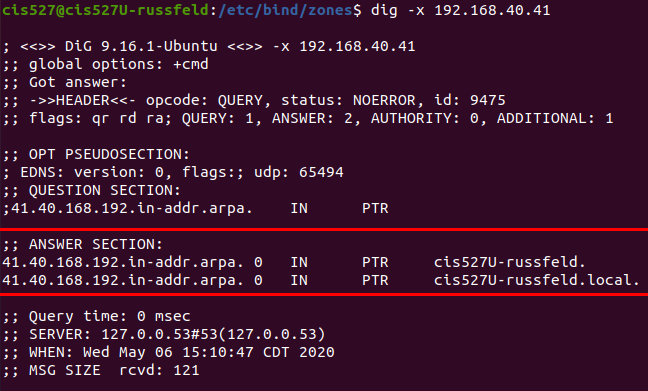
In this screenshot, I attempted to do a reverse lookup of 192.168.40.41, which should resolve to ns.cis527russfeld.cs.ksu.edu. This test was done from the machine with that IP address. Unfortunately, my server was misconfigured, and the reverse zone file was not properly included (the path in my named.conf.local file had a typo, to be exact). Since that file was not availble, my system returned the response from it’s local DNS information, showing that the IP address 192.168.40.41 belongs to cis527U-russfeld., which is the name of the actual computer and not its name in the DNS system. This can happen if you try to request information about the local system and the DNS server does not contain the correct information.
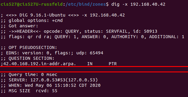
With the same misconfiguration as described above, when I query a different system, such as 192.168.40.42, I instead get an empty response as shown here. This is the usual situation if the DNS server is misconfigured and the PTR record cannot be found. If the output of dig is missing an answer section, it usually indicates that the lookup failed.
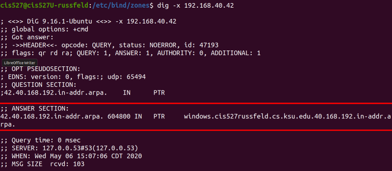
So, I corrected my error and restarted my bind9 server, and once again tried to query one of my reverse lookup addresses. However, in this case, I did get a response from the DNS server, but it was incorrect. The address returned when I queried 192.168.40.42 as windows.cis527russfeld.cs.ksu.edu.40.168.192.in-addr.arpa, which is not what I wanted. This can happen when you forget to add the all important period at the end of an entry in your zone file.

That one, right there. If you forget that one, the bind9 DNS server will automatically append a whole bunch of domain information after the address. Sometimes we want that, but in this case, we don’t. So, be very careful and don’t forget the periods.
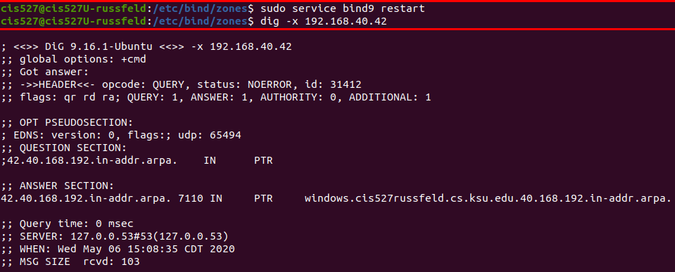
In this screenshot, I had just resolved the error above and restarted my bind9 server to load the newly changed files. Then, I once again used dig to query 192.168.40.42, expecting to see the correct output. Instead, I still received the incorrect output as seen in the screenshot above. This is a very common problem!
There can be a couple of causes of this issue. First, whenever you update a zone file, don’t forget to change the serial value to a larger number. The DigitalOcean guide just has you start with 2 and go to 3 and so on. I like to use the date, followed by a serial for that day. So, I would use a serial such as 202005061 for the first update made on May 6th, 2020 (2020-05-06).
Secondly, even if you remember to do that, many modern systems employ some form of DNS caching that stores the responses from previous queries. Both Ubuntu and Windows do this automatically. So, you may also have to clear your DNS cache to make sure it is properly querying the server. On Ubuntu, use sudo resolvectl flush-caches and on Windows use ipconfig /flush-dns.
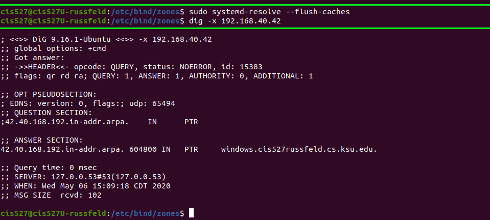
Immediately after flushing the DNS cache, I was able to perform the query again and get the correct result.
Below are screenshots showing correct output for various dig commands. You may use these screenshots to help in your debugging process. To take these screenshots, I updated the static IP address configuration for the Ubuntu Server to use it’s own IP address 192.168.40.41 as the only DNS server.
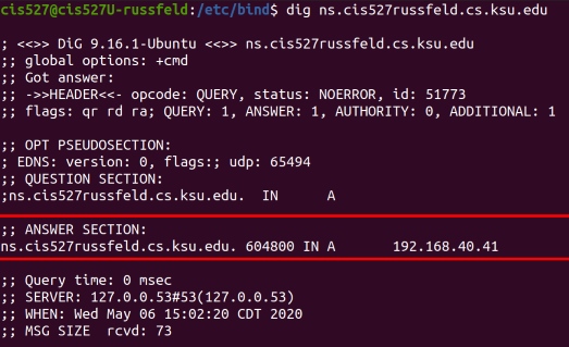
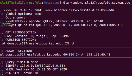
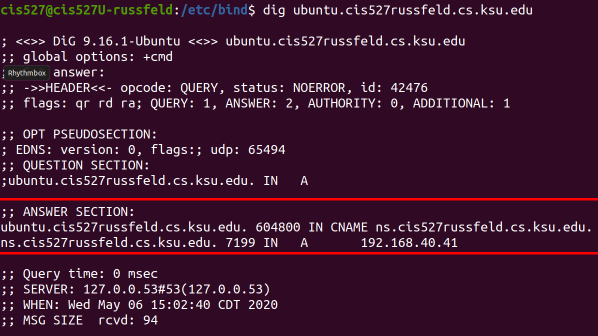
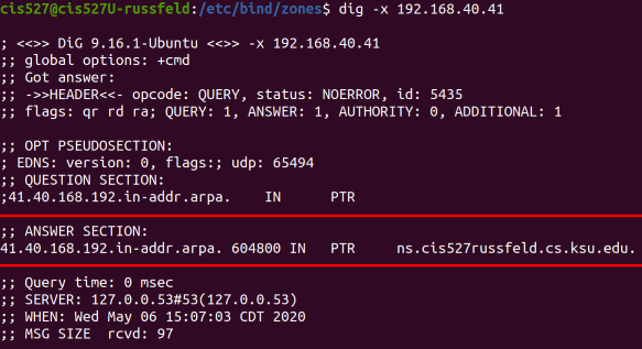
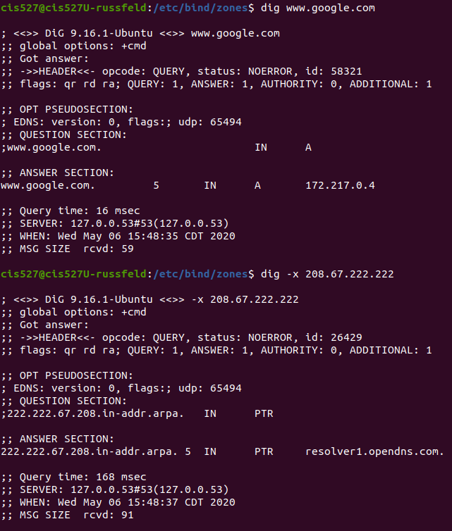
This is for an older version of Lab 3, but the basic idea is the same. You may have to update some details such as the network IP addresses and hostnames to match the current instructions for Lab 3.
Okay, so I’m going to try and talk through a model solution version of lab three and give you some advice on how to go about this lab. And also how to verify that you got this lab configured and working properly. So the first thing we’re going to do is we’re going to look at our IP address. So I’m going to go to the Edit menu in VMware and then choose virtual network editor. And in the virtual network editor, we’re going to find our NAT network. And we’ll notice that it has a subnet address of 192.168.40.0, yours will probably be similar, but it may have a different third octet right here. It’s usually randomly assigned by VMware when you install it. Mine is dot 40. Yours might be different, so we need to make note of that IP address. The other thing in here we can see is this checkmark the use local DHCP service; once you get done with task four and have your DHCP server running, you’ll want to go in here and uncheck this box, you have to click this change settings button to give it admin access. But then you can uncheck this box to turn off VMware’s DHCP service, so you can use your own. So remember we have 192.168.40.
So up here in Ubuntu, we want to set a static IP address in that same range. So in my settings, if I go in here and look at IPv4, you can notice that I’ve set an IP address 192.168.40.41. And the dot 41 is what the assignment says that we’re going to use for our Ubuntu server. We also need to set the gateway. In VMware, it uses a default gateway of dot two inside of your network. The reason it does this is dot one is usually used by your home routers and some other services. And so to avoid any conflicts, VMware has set it to dot two. We also have the netmask of 255.255.255.0. That’s pretty standard. We talked about the lecture. And then you notice that right now I’ve actually set it to refer to itself as a DNS server. Originally in the lab, you’ll probably set this to dot two, so that you still have working internet. But once you get your DNS server working, you can set it to dot 41. So that actually refers to itself for its DNS. So we’ll go ahead and apply this once you apply it, you can turn it off and turn it back on to make sure it’s applied.
This is the only VM in this lab that you need to set a static IP address on. I’ve seen some students try and set static IPs on the Ubuntu and the Windows, you don’t need to do that. For testing of your DNS server, you can set a static DNS entry temporarily. But the idea is by the time you get done with lab three these to your Ubuntu client and your Windows client should both be getting its IP address from the DHCP server on your Ubuntu server.
Okay, so once we have that set, we can confirm our IP address is correct by doing ip addr show that will show us our IP address. And we’ll notice right here that we see the 40 dot 41 IP address. We also need to keep in mind this ens33. This is the name of the interface that this is connected on. And so in the DHCP setup, you’ll need to go in and set a file that defines which interfaces to listen on. This is the interface we want to listen on. But for the DNS server, we actually tell it the IP address that we want to listen on. And so we’ll need this IP address in our DNS server configuration.
So once we have our DNS server up and running, we’ll also need to make sure that we allow it through the firewall, I’ll leave that up to you, you can look up what ports you need and how to allow that through the firewall.
But if it’s working, we can use the dig command followed by an at symbol and the IP address of our system. And so what this does is this tells dig to ignore any DNS settings we have on our system and query this particular server, and we’re going to query for ns.cis527russfeld.cs.ksu.edu. And when we do that, we get this response. Here, just to help. Let me put this command back up here again. So I’m doing dig at the IP address of my server. And you can do this either on the server or on the client. And then I’m giving it the name of a server that I want to look up in our DNS configuration. And so if I run this command, in this answer section, I should get back that this name goes to this IP address, which is correct. So that’s how we look up an entry on our forward zone.
If we went to look up an entry in our reverse zone, instead of doing the name, we do dash x, and then we would put in an IP address, I’m going to put in the IP address 42 which when we do this, it will show our answer section is we’re looking up 42.40.168.192.in-addr.arpa, which is the reverse lookup IP address. And then we are getting our Windows Server back.
So to really check to see if your DNS server is working, those are the two commands you need. You just need to be able to use dig at your server’s IP address, and then dash x for reverse lookup, or for forward lookup, you just put in a domain name. You can also test your forwarding. If you want to make sure your forwarding is working, I can dig that server and just look for www.yahoo.com for example, and I can get responses from that. I can also look up the reverse. If I want to look up a reverse, I can do a reverse for 208.67.222.222 which is one of the OpenDNS resolvers. So this is pretty much confirmed that our DNS server is working on the server.
If you want to check it from one of your clients, you can switch over to your client, and here on the client I can run those exact same commands. So if I do dig at my server IP address, and this is without setting any static DNS entries, this is just telling dig to query this IP. And then if I do my address here, then I can run it. And once again, we’re getting that answer. And so this is how you can check, you can test your DNS configuration before you have DHCP working, you don’t have to change anything on your client, you just use the at symbol in your dig command to tell it to query that particular DNS server for this entry.
So that’s the DNS parts. If that doesn’t work, there’s a really good guide on DNS troubleshooting that talks you through a lot of different things you might run into, Be especially careful of your periods and your spacing in your DNS configuration files. All of that is really important. There’s also a really good discussion on Piazza right now about the number of octets in your reverse zone file. In the dot local file, you can have three octets and then you only need one octet in your zone file. If that doesn’t make sense post on Piazza, let us know. We can try and clarify that.
Okay, so the second part is your DHCP server. And the DHCP server configuration is pretty simple. However, I’m going to call out one thing real quick. If I go to /etc/default, you’ll notice there’s a file in here that might exist. That’s, whoops. Helps if I go to the server. I go to the server. And then looking here, you’ll see there is a file called isc-dhcp-server. And so in this file, it has some entries. And depending on what guide you read, sometimes you will need to define an interface right here that your DHCP server could listen on. Mine I didn’t need to define that, it just worked. But in a lot of cases, you might need to define that. So this is where you would put that is that ens33 that we saw earlier.
So once you get your DHCP server running, you can start it, I’m just going to restart mine. So I restart that. And now your server should be running. If you want to check, a good way to check is you can do sudo cat /var/log/syslog. And we’ll look at the very end of our syslog. These last few entries. And we can see here that our, that our DHCP server started up; it read its config file. And then it will say things like listening and sending. And as long as you see that it’s listening on ens33. That means it’s working. If you get an error here that says it doesn’t, it’s not configured to listen on any interfaces, that’s where you might need to change that defaults file to listen on ens33 to work. So. That’s how you can tell your DHCP server started correctly.
There’s a couple other commands that you can use using the ss command to look at listening ports. So ss -l will show you all the listening ports on your system. However, it’s not very useful at all. So instead, we can try two different versions, I’m going to do ss -l, then I’m going to do t which will listen for TCP ports only. And then n which will show us the port numbers. So if I do ss -ltn, I will see really quickly that I have a DNS server listening right here on port 53. That’s what we’re looking for for DNS. DHCP, however, is not TCP is UDP. And so if I look for UDP, I’ll see a DHCP server listening here on every IP address on port 67. And so there is the entry for your DHCP server. And so if you’re not sure if your servers are running correctly, you can use ss -ltn or ss -lun and look for entries that end in 53 for your DNS server or 67, for your DHCP server.
You’ll also notice that there is 161 for your SNMP server if you have that running. So this is kind of a really useful thing. You can also see your SSH server running on 22222, and we’ll see our HTTP server Apache running on port 80. So a couple of quick commands.
But the really easy way to test your DHCP server is actually on Windows. And so on Windows, I have no static IP address set. If I do ipconfig /release, that will release all of our IP configurations. And then I can do ipconfig /renew to force it to renew that IP address. And so it will think for just a minute and then it will come back and it should give us an IP address that has something within our range. It has dot two as the gateway. But the big giveaway is you can find this connection-specific DNS suffix, and it will contain your eID. That’s the dead giveaway that you are getting a DHCP address from your DHCP server. And that’s why it’s actually really easy to test this on Windows.
Now, if I do ipconfig /all, then it will show all the information. And you can see that it also is getting the DNS server for your network. And so it actually gets the right DNS server, it will also show you what your DHCP server is. So if you want to know where that IP address came from, you can find it here as well. And then, of course, we can use nslookup to look up different names on our network. So if I do nslookup, I can look that up. And if I do the reverse, I can get the reverse as well. So everything is looking really good here.
The other thing you can do, obviously, for testing is on your Ubuntu client, you can do sudo dhclient -r, which will run the DHCP client and refresh. If I do sudo dhclient -v, you’ll actually see it sending the DHCP discover. So it sends to discover, then we get an offer of this IP address from our server IP. And you can see that it works.
So those are a quick overview of what lab three should look like when it’s working correctly. The big things to do are get your DNS server up and running, and then test it here on your server using those dig commands with the at symbol on them. So if we go back through my history, we find some of these dig commands having the at symbol where we can query a particular DNS server and look up a particular address. Once you get that working, you can then test it from your client using that same syntax or you can just go ahead, get your DHCP server up and running, check the system log to make sure it’s running. And then go to your Windows client, reboot it and make sure that it’s getting an IP address from your system. And then you should be good to go.
If it’s not working, check your config files, check your firewall, make sure that it’s listening on the right ports, or feel free to reach out on Piazza and let us know. So I hope this video was helpful. If you have suggestions or questions or anything else I can go over please let me know.
Good luck.
Here are some helpful networking diagrams to better explain the desired state before and after the end of Lab 3. In all of these diagrams, I am using a sample network with the IP address 192.168.40.0. You will have to adapt the IPs to match your network configuration. In addition, each network address will need to be updated with your unique eID as directed in the lab assignment.
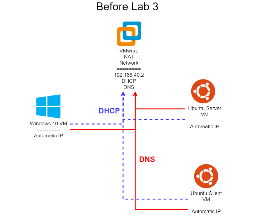
Once you’ve completed Task 1 of Lab 3, you should have three virtual machines connected to your network. Each of them will be configured to automatically get an IP address using DHCP, and they will also be configured to use the automatically provided DNS information from that DHCP server. By default, the NAT network in VMware is configured to use VMware’s built-in DHCP server to handle automatic IP addresses, and that DHCP server also configures each system to use VMware’s built-in DNS server. That server can be found at 192.168.40.2.
This is very similar to how most home networks are configured, where the wireless router acts as both a DHCP server and DNS server (in actuality, a DNS forwarder, since it doesn’t really resolve DNS entries itself).
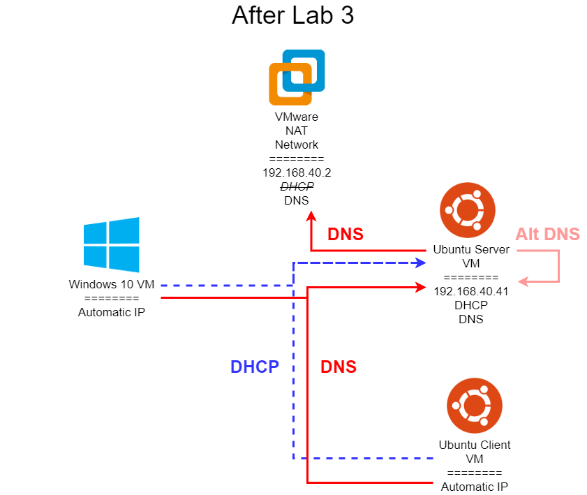
Once you’ve completed all of Lab 3, your network diagram should resemble the one shown above. At this point, you have installed and configured both a DNS and a DHCP server on your Ubuntu VM labelled Server, and disabled the built-in DHCP server in VMware’s NAT network. By doing so, your Ubuntu VM labelled Client as well as your Windows 10 VM will now be getting automatic IP addresses from your Ubuntu server. In addition, the DHCP server will configure those systems to use your Ubuntu server as the primary DNS server. So, whenever you try to access any addresses in the cis527<your eID>.cs.ksu.edu network on those systems, they will use your Ubuntu DNS server to look up the names.
However, notice that your Ubuntu VM labelled Server still uses the VMware DNS server as its primary entry. By doing so, it will not be able to look up any addresses in the cis527<your eID>.cs.ksu.edu network at this time. However, you can modify its DNS settings to include a secondary entry which points back to itself (it is important to use it’s external 192.168.40.41 IP address for this, and not the localhost address 127.0.0.1). By doing so, that will allow it to query itself for DNS entries it can’t find, but will still guarantee it can access the internet even if your internal DNS server is not configured properly.
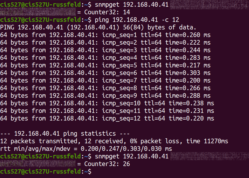