CS Concepts
The basic building blocks of computer science theory and programming, along with a bit of history!
The basic building blocks of computer science theory and programming, along with a bit of history!
In this module, we will dissect what computing science really is. To do this we will step back in time to determine what the motivation was for computing machines, the products of those needs, and how they served as inspiration for modern computing.
In this course, we’re going to ask ourselves, what is computing science? It’s a really important topic that we’d like to cover throughout this course. But it’s also one that’s very difficult to understand. So when we try and understand the topics such as what is computing science, we can ask ourselves the questions: who? what? when? where? why? and how? And while I do this, I realized the question of “how” is really the best way to approach computing science. Specifically, I like to think of computing science as the study of how - how we can make things faster, better, more efficient, more accurate and more secure using computers. But that becomes a really interesting statement because we haven’t discussed exactly what a computer is.
So before we can look at all this “how”, let’s ask ourselves: “what is a computer?” We’re all probably familiar with the modern computers that you and I have in our homes and around us today, but is that really the best definition of what a computer is? Or is there more to it? That’s what we’re going to take a look at in this video. So to really understand what a computer is, we have to go back a little bit and look at some of the earliest examples of devices that might be considered a computer. And it turns out those devices are really wrapped up in the history of mathematics.
So on this slide, we see some mathematical equations, such as the equation for the exponential function, which is this long, repeated division. We can have sine and cosine and all of the trigonometric functions. We can have limits which are the basis of calculus, and we can even have logarithms which show up a lot in statistics and finance. And all of these functions are very, very difficult for people to calculate by hand. So how do we find the values of, for example, sine of 46 degrees? Using modern technology, we can find these values using some very interesting tools such as computers or calculators, but in the 1600s, they might have to use something such as this.
This is a book of math tables from 1619, and it gives the value of sine, tangent, secant for all sorts of different angle values. And so a table such as this might be used by engineers, mathematicians and scientists whenever they need to find these values for their work. And in fact, if you’ve taken a calculus class, or trigonometry class or geometry class, your textbooks probably had tables like this in the back of the book. And as recently as the 1960s and 1970s, engineers would have had little books full of these tables that they carried with them all the time before the rise of the modern pocket calculator. But of course, this begs the question of how do we get these numbers in these books? We don’t have computers, we don’t have calculators.
So how did we do it? And it turns out that that lies in the work of a lot of early mathematicians such as John Napier, who helped describe the logarithmic function, and Jacob Bernoulli, who helped describe the exponential function. And so one way that you could populate a book full these values is work with the best mathematicians at the time and have them perform all of that mathematical work. And this is important because in the 1600s, not many people had the level of mathematical training required to work with those really complex functions that we saw earlier. But of course, this is not a really great use of their time. So we tried to find ways where we could do better and easier mathematics to find those complex values.
One of those big improvements was the creation of Taylor series. If you ever take a calculus class, you’ll learn all about Taylor series. But the big thing to understand is a Taylor series is simply an infinite polynomial that expresses values of those complex functions. For example, the exponential function can be expressed as the infinite polynomial, one plus x plus x squared over two factorial plus x cubed over three factorial. And so we’ve reduced this value down to a set of individual terms. And so if we can calculate the value of each individual term and add them together, we can find the values for the exponential function. Of course, this is a little bit easier than that earlier statement, but it’s still very, very complex mathematics that would take a lot of work.
Enter the work of Sir Isaac Newton, Isaac Newton, you’ve probably heard of lots of times in your math and science courses, and he was very impactful in a bunch of different fields. But for this particular field, we’re looking at one specific thing he created that’s not very well known, which is the method of divided differences. And so Newton’s method of divided differences allows you to find successive values of a polynomial, any sort of polynomial that you can create, including these infinite polynomials for Taylor series. You simply cut them off at a particular value, and then you use that polynomial and Newton’s method of divided differences to find those values that you would place in a book. So let’s look at an example of Newton’s method of divided differences to see how it works.
To understand Newton’s method of divided differences, we have this example with a polynomial: two x squared minus four x plus three. Then we’ve created a table below, where we have the first column that gives values of x and the second column that gives values of the polynomial applied to that value of x. So for example, if we put x equals zero into the polynomial, we’ll get the value three. If we put x equals one in the polynomial, we’ll get two minus four plus three, which is one, and so on. So we can populate the first few values in this polynomial column very easily using simple mathematics.
Once we’ve got a few of those values, then we can build this first differences column. And so the differences column will take the value of the polynomial at one minus the value of the polynomial at zero, and so we’ll have one minus three, which will give us negative two. Likewise, for the next value, we’ll take three minus one, and we’ll get the value two. And so we can do that to fill out the first few values in this difference column.
And then we’ll do it again to make a second difference column. So here we have two minus negative two, which is four. And what Newton realized is if you do this enough times, you’ll eventually reach a column where all the values will be the same. And you have to do that for each order of the polynomial. So this is a polynomial of order two. So that means we need two division, or two difference columns to get to this column, where all the values will be the same. So now, once we know that this column is four, we can put in four for each of these values.
And then we can use those to work forwards through the table to find other values of the polynomial. So now to fill out this value right here, we can do four plus two, and we’ll get six. Then we can do four plus six to get 10 here, then we’ll do four plus 10 to get 14, then we can work forward again and fill out the polynomial column where we have six plus three is nine. 10 plus nine is 19, and 14 plus 19 is 33. There we go. That’s how you do Newton’s method of divided differences.
This slide shows a completed table that is a little bit easier to read. And we can see that we got the correct values. Now this method of divided differences does have one major issue, and that is it’s very susceptible to human error. For example, what if we add four plus six and instead of getting 10, we get 11. Then what happens? Well, if we do four plus 11, here, we’ll get 15 instead of 14. Then if we do six plus three, we get 9, 11 plus nine, now we will get 20 here. And then likewise, if we do 20 plus 15, instead of 33. We will get 35. And so as you can see, by making one small error right here, we’ve actually made all of the subsequent values in the table invalid. And that’s the real problem with Newton’s method of divided differences. As soon as you make one error, it invalidates everything after it. So while it’s a very powerful tool, it still has a big weakness.
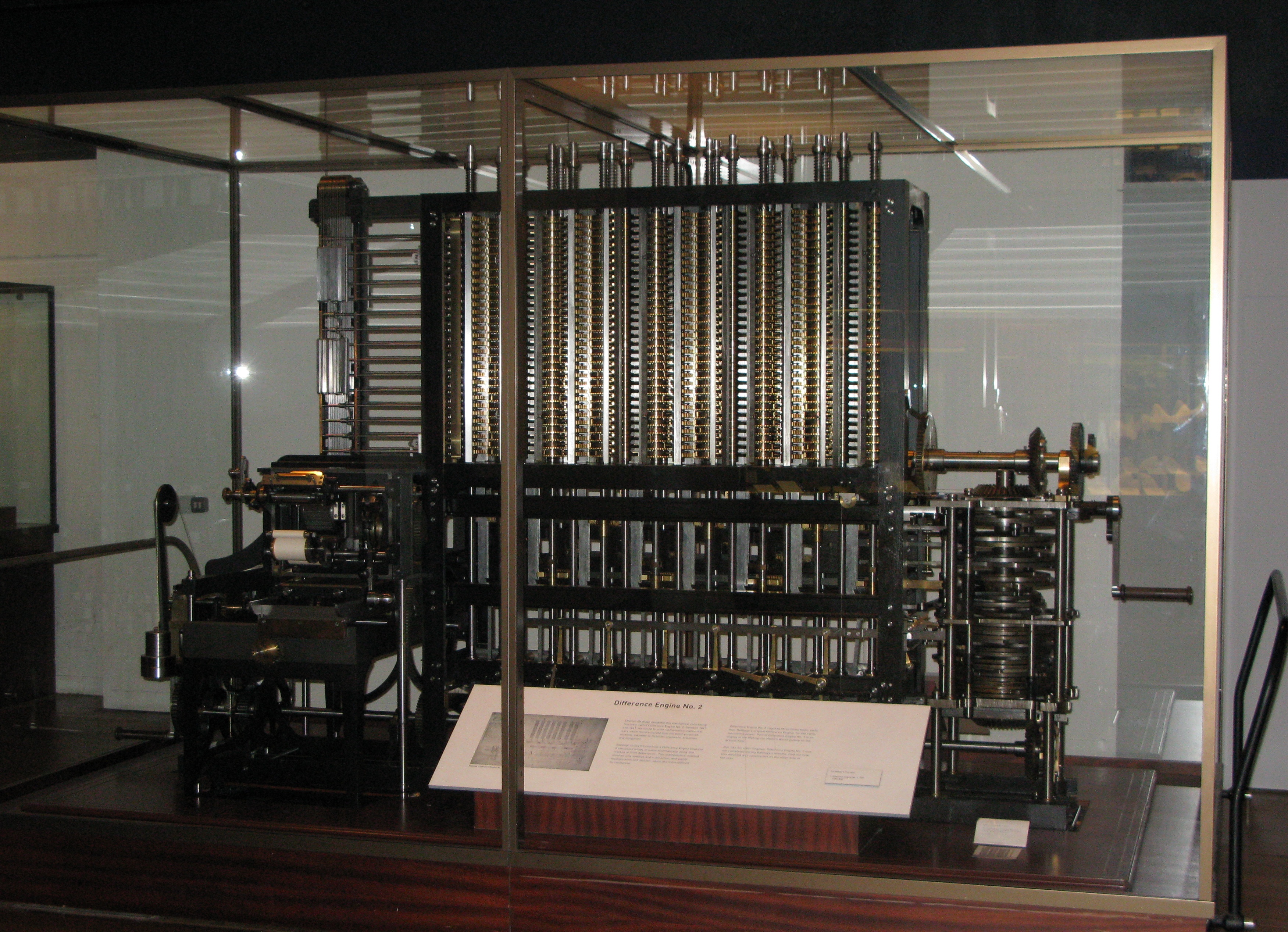
And the real idea is how can we solve this weakness. And that was of interest to Charles Babbage. Charles Babbage was an inventor and a mathematician in England in the 1800s. And he was really interested in creating ways that we could perform these repeated calculations without the risk of human error. And he decided that it was possible to build a mechanical device that could perform these mathematical operations completely, repetitively without any error. And during his lifetime, he actually built a small prototype of this device that he called The Difference Engine, and he built blueprints for a much larger scale version of it, but that version was never actually completed during his lifetime. A few years ago, those blueprints were in the possession of a Computer History Museum and they decided to try and build a device based on his blueprints and see if it would actually work. And surprisingly enough, it totally worked. So let’s take a look at a video of that completed Difference Engine that was built by a Computer History Museum and see how it works.
The director of the Computer Science Museum’s Babbage Project demonstrates how Charles Babbage’s Difference Engine #2 works. While Babbage himself was not able to build the machine in his lifetime, a modern builder created it according to Babbage’s instructions. Through this creation, computer scientists have been able to prove that the Difference Engine works exactly as Babbage intended!
WIRED. (2008, May 2). Babbage’s Difference Engine No. 2 [Video]. YouTube. https://www.youtube.com/watch?v=0anIyVGeWOI
Charles Babbage designed many different engines during his lifetime, but very few of them were actually built.
In the previous video, you saw a completed version of the Difference Engine built very recently, which we actually see here. And his Difference Engine was very revolutionary because it proved that you could build a device that was purely mechanical, that could perform calculations. But the difference engine was actually a very small part of Babbage’s overall vision for building these mechanical computational devices.
He also designed another engine that he called the Analytical Engine, and it was never completed during his lifetime and thus far it has not been completed in modern day time either, but there are small parts of it that exists. For example, this is one small part of it that is in a museum. The analytical engine would have been a true multi-purpose computer. Instead of just performing Newton’s method of divided differences, it was capable of performing all sorts of different mathematical operations.
Babbage’s Analytical Engine would have been programmed using input cards, such as what you see here. And one surviving portion of the Analytical Engine is the Mill, which is a general purpose computational device that can perform all sorts of different mathematical operations. It’s very similar to the CPU in modern computers.
In addition, he would have created a device called the store, which was capable of storing and retrieving up to 1000 numbers at 40 decimal places, which is roughly 16 kilobytes of data, which is really respective for the 1800s. And parts of the design for the store were actually used in the design of the Difference Engine, which is the picture you see here. So what have looked very similar.
And so because of all of his work, designing and thinking about how you would build these multipurpose computational devices, we refer to Charles Babbage as the father of modern computing. Unfortunately, a lot of his designs were forgotten over time. And it wasn’t until very recently that his work was really recognized as being so revolutionary in the history of computing science. In a later lecture in this class we will actually analyze some more work of Charles Babbage, specifically the Analytical Engine, and how it fits better into the history of computing science.
Read Pattern on the Stone, Chapter 1 - Nuts and Bolts.
“The Pattern on the Stone: The Simple Ideas that Make Computers Work” by W. Daniel Hillis. ISBN 046502596X, newer version is also available and will work fine
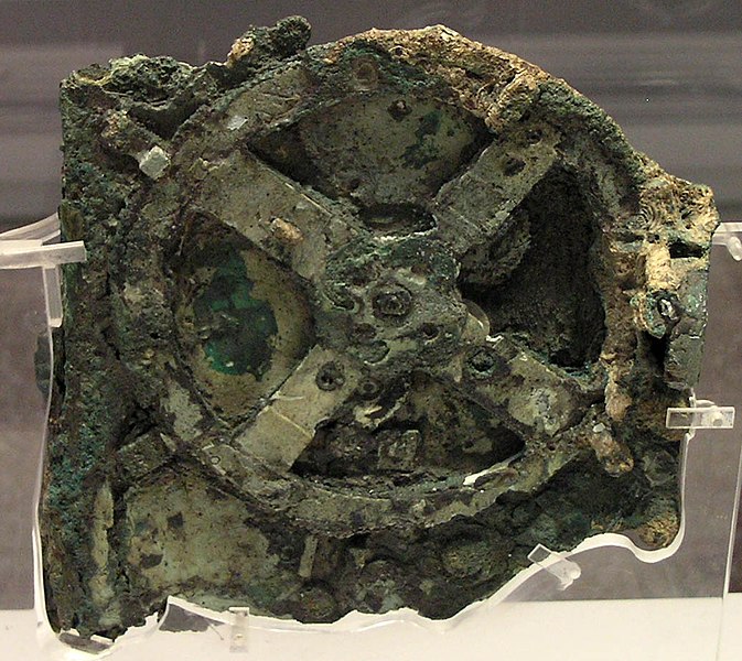
This video outlines how the Antikythera Mechanism was found and some of the research that has been done on the mechanism. Getting its name from the island by which it was found, the Antikythera Mechanism had been hidden in the ocean for over 20 centuries. This is a textbook example of how humans have been automating processes for thousands of years. This video offers an insightful juxtaposition of using modern computers to analyze ancient computers.
Antikythera - Anticythère - Αντικύθηρα - 安提凯希拉. “The Antikythera Mechanism - 2D”. June 25, 2011. YouTube. Available: https://www.youtube.com/watch?v=UpLcnAIpVRA.
Today we’re going to be learning about historical computing machines. Now, computers like we know today with your electronic laptops and cell phones and everything aren’t just electronic, but really anything that can compute a value, whether it be mechanical, electrical, or even biological. What we’re looking at here is a piece of what is considered one of the oldest computing machines that we know of the Antikythera mechanism. It was discovered in 1900 off the coast of a Greek island called Antikythera and really is puzzled scientists for quite some time. It was believed to have originated around 100 BCE, but little was known about its origin. But however, from the detailed gears and inscriptions on the piece itself, we can actually deduce what it is actually used for. As you learned in the video, the Antikythera mechanism was an early computer used to calculate the position of the sun, moon and planets in the sky, as well as important dates and eclipses. Now, after this period of time, it wasn’t until the 14th century that mechanisms of this complexity were ever seen again, though this was completely beyond its time in terms of technology.
The Abacus is another early example of a competing machine that you’ve probably seen and heard of, or maybe even used. They’re now used a lot as a children’s toy. But this is an example of a Chinese Abacus. With a little bit of technique and training, this device allows the user to perform addition, subtraction, multiplication, division, and even the calculation of squares and cube roots at pretty high speed once you get used to it. But even with that, this machine still has a still has some room for human error, which is really what the the crutch of a lot of these devices are.
But moving forward a few hundred years, in the early 1600s, the slide rule was invented. It uses a sliding set of logarithmic scales, and allows the user to calculate all sorts of values from simple multiplication to logarithms and even trig functions. And for students studying engineering through the 1960s it was the tool of choice for those calculations needed until the calculator or the electronic calculator started to catch on and become small enough and useful enough for it to pretty much overtake everything else that we have used so far. Even though the slide rule is this simple device, it was used for even things like the Apollo 13 launch and if you’ve ever watched Apollo 13 before you can kind of see through this particular clip of the slide rule being used to verify some calculations.
Now that we have an understanding of the resources available at the time, let’s take a step back and think about what it would be like to be an inventor in let’s say the 1600s for a minute. If you wanted to design a machine that would aid in the computation of complex values, what should it do? What does that mean for a computer? Right? If we’re trying to avoid a lot of the human error that we have in calculating specific values, or make our lives easier, what should that computer what should that device actually do?
Based off of that discussion, or based off of that thought, I’m going to suggest four different things that a modern computer should be able to do. It should be able to compute some form of complex value and not just one calculation, but many, many types of calculations. It should be able to accept variable input. So not just a simple calculator that can accept numbers, but accept all sorts of different things like even a program, for example. It should be able to store information and should also be able to output that information as well. Because what’s the point of computing something if you can’t actually see what the result is? So you might see that many of these actually compared to the functions of computers today, right? The processor, a CPU that can compute value, programs for variable input, your RAM or your hard drive for storing information and your monitor or your printer that can output the results. Before we go further, right we need, we’ll need to figure out some way to compute values. And as we discussed earlier, human error is a major problem here. So regardless of how well the machine is capable of computing those values, we need to reduce or eliminate that factor of human error. So we want to design something that doesn’t have any humans involved in the calculation. Because if there is, like the abacus or the slide rule, the result is only as good as the person actually operating the machine.
So one step into that in 1642, Blaise Pascal invented the mechanical calculator to solve that problem. And now it was originally designed to help his father calculate tax revenues and of course if you know a little bit of history during that time period, taxes were pretty big deal and you know, if you collected too much from your townspeople, right, everyone grabbed their pitchforks and torches, and if you were the guy collecting taxes, if you didn’t collect enough, the king would go, you know, off with your head, that sort of thing, right? So this is a pretty big deal. Any sort of error could really literally mean life or death. So this machine was capable of addition and subtraction and could simulate multiplication and division by repetition. So, you know, essentially the beginnings of the calculator that we know and use today. Unlike the abacus, there’s much less room for human error. Here you input the numbers, and out come a result.
To further improve on Blaise Pascal’s design, in 1673 Gottfried Leibniz created a stepped drum, commonly referred to as a Leibniz wheel that greatly increased or enhanced the capabilities of any mechanical calculator that used it. With the innovations of these two guys here, the Pascal and Leibniz, the world now had the capability, at least the mechanical capability, to perform calculations.
That really led to Charles Babbage. And now in 1823, Charles Babbage designed his first Difference Engine, and built the prototype that was showcased in his study in his home for quite some time. Now, this is the, the larger version of that prototype, but the difference engine itself was capable of simple mathematics and could solve even polynomial equations up to six digits. So, this was a huge step forward, but it was only a small part of what Babbage had actually envisioned. The Difference Engine is what we call a fixed program or a single purpose computer, meaning that it could only do the task that it was built for; it couldn’t be reprogrammed to do anything else like our modern computers could. The Difference Engine could calculate the value of any seventh order polynomial, given the correct input by using method of finite differences. While the differentiation itself in its entirety wasn’t built during his lifetime, Babbage’s idea here was really truly revolutionary.
While the creation on Babbage’s Difference Engine #2 was turned down by the government, we get to see this machine which was built in modern times. Babbage had a small prototype which he would demonstrate for party guests and it was clear to those who saw it, that Babbage was incredibly talented and intelligent. This is further proven by the prototype’s modern counterpart. It is astonishing that it was created with such precision using just pencils and paper!
Computer History Museum. “Charles Babbage and His Difference Engine #2”. May 5, 2008. YouTube. Available: https://www.youtube.com/watch?v=KBuJqUfO4-w.
In this video, we get to see another example of antique computers! Created in 1803, the Jacquard loom used technology that would be a predecessor to the more modern punch cards and in turn, modern computers. As before with the difference engine and the Antikythera mechanism, this was a result of humans trying to automate tasks which required a lot of precision.
The Henry Ford. “How an 1803 Jacquard Loom Led to Computer Technology”. July 27, 2018. YouTube. https://www.youtube.com/watch?v=MQzpLLhN0fY.
So now that we have the capability of computing values without human error, once we have that ability, the next important part of the computer is to accept variable input from the user. And as I mentioned before, it’s not just the fact that we can input numbers into the computer. But, what if we could actually reprogram the device? Right? What if we could enable certain features or certain abilities of that computer by just pushing the input?
Can anyone guess what mechanical device was the first one to accept variable input from a user? It was the Jacquard loom. Not a whole lot of people know about the Jacquard loom, but it was invented in 1801 by Joseph Marie Jacquard, who basically simplified the process of manufacturing textiles. Particularly with textiles that have really complex or shifting patterns or even rounded designs and things of that nature. The Jacquard loom used a series of punch cards to control the thread. While this doesn’t actually perform any calculations, it is very important as this is the first example of a machine responding to different input or programs in the form of punch cards. Now, the car loom wasn’t the first thing that ever used the idea of punch cards. There was a few things before its time, but there’s Jacquard loom was one of the first one that truly automated the process. Although there were still some manual aspects of the Jacquard loom, the majority of it was completely automated.
The Difference Engine wasn’t the only computer designed by Babbage. The Analytical Engine, which was Babbage’s true dream: a general purpose computer. Had it been built as Babbage envisioned, it would have been one of the first true modern computers. He previously worked on design of an analytical engine, which was a true multi purpose computer. It would have been composed of several different parts that each performed different functions, allowing it to do many different kinds of calculations, be reprogrammed, store information and all sorts of different things. This was one of the first steps that we have seen, be developing or to developing a true modern multi purpose computer. Analytical Engine used a set of input cards called punch cards to determine what calculations to do and what numbers to use. And so this was greatly inspired by the Jacquard loom. This is very similar to how programs on today’s computers are structured: with a list of instructions on the program or in the program and the data that’s provided by the user.
Borrowing that idea from the Jacquard loom, the analytical engine was able to use a system of punch cards to accept input and determine the calculations that needed to be done. Babbage’s son remarked once that the Analytical Engine could calculate almost anything, it is only a question of the cards and time. So how many cards it would require and the amount of time it would take to actually operate, speculating that 20,000 cards would not be out of the question. It was a pretty impressive physical mechanical machine. This is very much like how modern computers worked, and even in the 40s and 50s a lot of computers worked off of this punch card system.
In the Analytical Engine, there is also the mill. The mill is really the heart of the machine. I was equate this closer to what a modern CPU was. In order to handle the computation done by the machine, Babbage designed this part that was capable of performing all of the basic numerical calculations. This used many of the breakthroughs that Pascal and Leibniz had some 200 years earlier. And so here in this picture on the slide is a very small picture of one part of the mill, which was constructed actually by Babbage’s son in 1910 to show that it was actually possible. The mill is able to perform all the basic arithmetic operations like addition, subtraction, multiplication, division, as well as calculate the square roots of numbers. This is really the first true step towards a modern CPU, which is really exciting. With those two parts in place, the next big hurdle was the ability to store data and output the results.
The store was Babbage’s true innovation. The store, which would have been a bank of columns capable of storing up to 1000 numbers up to 40 decimal places each. So that’s pretty high precision for a mechanical device. This was equated to roughly 16 to 17 kilobytes of modern day storage if you want to look at it that way, so quite a bit. Now, while the store was never actually built for the Analytical Engine, much of the design for the store was incorporated into his Difference Engine number two design, which is shown here in this picture. This represents the first time that calculated values could be stored directly in the machine, and recalled at a later time as required by the program.
The last thing that our computer should be able to do is output results. Charles Babbage also thought of this, right. As we saw in the video, in our previous lecture, Babbage also designed a printer that would output the results of calculations, not only onto paper, but directly into a plaster panel that could be used to create printing plates. You can imagine using this device to maybe make all of those tables in the back of your mathematic textbook. Which were a pain to do by hand, but now we could have a machine that would actually do the math and print it as well.
Now what those parts in place the stage is really now set for the coming computer revolution. Unfortunately, it will take an entire world consumed by war before the next major step in the history of computing was made. And we’ll pick that story up in the next couple of lectures.
This really leads us back to Charles Babbage, the father the modern day computer, it’s really quite mind boggling to see the Difference Engine, Analytical Engine, the Difference Engine number two, really all of which you only completed a simple prototype during his lifetime. And the fact that he was able to create these devices completely theoretically on paper, and they worked as intended exactly how he designed them is really, really quite amazing. Charles Babbage is known as the father of modern day computer because of these devices that were really truly one of the first examples of a general purpose computer. But if you’re interested in learning more about Charles Babbage, you can read his autobiography titled, “The Passages from the Life of a Philosopher” which is free and available online.
This video gives a great insight into what we will cover in this course. Our journey will start with early computation tools, such as the abacus, slide rules, and astrolabe! We see punch cards as a connection between early computing and modern computing.
CrashCourse. “Early Computing: Crash Course Computer Science”. Feb, 22, 2017. YouTube. Available: https://www.youtube.com/watch?v=O5nskjZ_GoI

For this lesson, we’re going to be talking primarily about Boolean logic, Boolean algebra and how that plays into computer science and the foundations of how important that is and the role it plays and what we do. So before we get started, and before we can talk about things such as Boolean logic, we need to know where it came from. That leads us to Aristotle, way back in the 300 BC, as you may know, right Aristotle is one of the fathers of modern philosophy and logic among many other things. He studied under Plato, who himself was taught by Socrates and was also the teacher of Alexander the Great, so pretty much affected the entire world of Western philosophy that came after him. One of his major contributions was this idea of using formal logic to prove a point, then this form of logic, also known as Aristotelian logic, a point is proven based off of a series of premises.
For example, in this form of logic, we can present a series of facts. And so our premise here in that sense, all humans are mortal. Socrates is human. Each one of these is a fact and pretty easily proven to be true. Now, under Aristotelian we can use these use this premise to then prove a new fact. So if all humans are mortal, which is true, and Socrates is a human, which is also true, we can also prove or conclude that Socrates is also a mortal.
If we skip ahead a few thousand years later, we come to George Boole. In 1854, he published a book called An Investigation of The Laws of Thought, in which he tried to apply the rapidly growing field of mathematics to the laws of logic. His goal was to reduce something as complex as logic to simple mathematical equations. And with the right rules in place, even a complex logic Statement could be completely proved, or even disproved using the same algebraic techniques they used to understand other parts of the world.
And so if we take a look at an example, our same style of facts that we had before now transcribed into something that is more easily represented in algebra or mathematics, so for example, if we take are all humans are mortal and Socrates is a human, we can map that to different variables. And you can kind of imagine different kinds of facts being transcribed here where we can substitute proven facts or true facts in places of a and b and c, we can conclude new facts or new premises or new things from that. So if A and B so the upside down would be their means and we’ll talk about that here in just a little bit. But if both A and B are true, and B and C are true, we can conclude that A and C is true. Since A and B are true, B and C are true, then A and C must also be true. But this translation is somewhat flawed but we can leave that for a later course in logic or philosophy to describe why …but let’s take a deeper dive into what each of these mean so primarily Boolean operators Boolean values and what that means for Boolean logic.
As you know from the reading computers operate primarily using only binary values so ones and zeros and Boolean logic and Boolean algebra operate off of true and false principles or yes no answers but that in itself is a binary decision there is no in between. So we can easily translate binary and Boolean logic back and forth. Commonly speaking, one is going to mean true and zero is going to mean false. Now, this is the same thing is translated in a variety of other contexts, like electrical systems where a on or off signals being produced one or on meaning electrical current, or off or zero. meaning no electrical current. So while these are traditional representations in many electrical and programming contexts, these values can be reversed for a variety of reasons. And really the moral of the story here is make sure you know which one you’re working on.
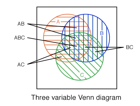
Let’s take a look at what the Boolean and operator does out in this Venn diagram here we’re going to kind of use these to showcase where the Boolean statements that we’re checking out with the Boolean operator where these statements are actually evaluated to be true. So if we assume that we are two facts here, A and B are both true. So let’s say this inner circle here, this left circle here represents a and this right circle here represents B and the square on the outside represents everything else. So when a and b are not, so if A and B are both true, then the statement evaluates to true. So the left hand side and the right hand side of the operator both must be true in order for the whole statement to be true. If A is false, or B is true. false, then the whole thing would be false. Now if we introduce a third fact, see, we kind of get the same results, right. So similar kind of story with the Venn diagram. Here we have a, b, and c. But notice that this little square here where we were actually filled in over here is no longer filled in. And that’s because all three facts must be true for the whole statement to evaluate to true. So a has to be true, B has to be true. And C has to be true in order for the whole statement to evaluate true.
So we’ll have similar representation here for the OR operator where the English word is the representation in Python of the OR operator the double bar symbol, so this is just the two vertical bars from your keyboard that is the OR operator in Java, C sharp and other programming languages and then a capital V is great. To be the OR operator for Boolean algebra. So let’s take a look at how or operates. So if we have the same statement, as we have before the same two premises A and B both being true initially, and the circles are kind of the representation of the same thing here, but the OR operator will evaluate to be true if either side of the operator are true. So if the left hand side is true, or the right hand side is true, the whole thing will be true. So if A is true, or B is true, so left hand side and the right hand side, so if A or B is true, then the whole statement is also true. And so nothing on the outside will actually be filled in quite yet. And the similar kind of story is for a third fact or fifth, that one has to be true for the whole statement to be true. So if any of them are true, the whole thing is true, but things kind of get tricky when we’re in introduce this next operator the exclusive OR exclusive or you won’t really find normally in programming languages. The Exclusive OR can be simulated using and or and the next operator that we’ll be covering here in just a second.
But the exclusive OR works in a little bit of a different way than the regular or the exclusive OR operates very similar to what we would expect the normal or operator to be in the sense that if A is true, or B is true, the statement is true, but notice that a and b is now false. If a and b are both true, the statement is false. So the exclusive OR operator is expecting one or the other. So that means the left side or the right side must be true, but not both. That is where the exclusive portion of the exclusive OR or the X or operator actually comes out. If I introduce a third fact things get to be a little bit more difficult to understand because now I would expect it to be kind of similar pattern as we have up here just to be, or on my just with my two facts, everything in the middle would be white, but everything on the outside would be red. But you notice when when we have all three to be true, all three can be true and the exclusive OR would still be true. Now let’s take a look at why that would be the case.
So let’s take a look at the example that we saw on the slides. We have our facts a, and our XOR operator. So we have a XOR B XOR. See, now if we kind of do our substitutions here now we could substitute ones and zeros here are true and false. So let’s go ahead and substitute our Boolean values here for our variables. So if A is true So we have a XOR B, which is also true. And C, which is also true. Now, just like most of your math problems, even when you’re just doing multiplication and division, you’re always going to evaluate your statement from the left to the right. So we need to first evaluates true x or true now XOR Exclusive OR exclusive right, the left or the right can be true, but not both. Since the left hand side of my operation is true, and the right hand side of my operator is true, this portion of the statement evaluates to false. Then all we need to do then is keep on working the rest of our statements. So we still have one XOR left. So we have false x or true? Now exclusive or one side or the other must be true but not both. So false x or true is actually true because both sides aren’t true. So this statement you say a false x or true, evaluates to true. So the whole thing true x our true, false XOR true, ends up being true.
So our last Boolean operator here is the NOT operator. The NOT operator acts pretty much like negation, as you would expect, like multiplying something by negative one not something is the opposite of what it actually is in Python as the previous Boolean operators the and and the OR operator, the NOT operator in Python is very English light not but Python is kind of weird. You will also see the exclamation point In some operations, but it doesn’t mean the traditional knots or negation operator as in many other programming languages. So, again, you’ll see not in Python, the exclamation point, this is going to be things like Java. And the weird sideways l here, this is going to be your Boolean algebra. So let’s take a look at what the Boolean operator not actually looks like. As I mentioned, the NOT operator is a negation, so not something as the opposite. So not a or not true is false. So not a if I write a here, so everything in the circle is a so when A is actually true, so everything inside of the circle then everything on the outside of a is actually true because it’s negated and similar idea for B when B is true, everything But B is true. So the whole statement is evaluated as such and similar idea if I introduce a third fact. So if I have three facts A, B and C, not B means that everything but B is true, just like in this example here.
So with all these new tools, we needed some new algebraic rules to really deal with them. Thankfully, most of the rules you know, apply quite well, but there’s one rule that needed to be added. In mathematics. When you multiply by negative one, you have to change the signs. Similarly, Augustus DeMorgan came up with a way to deal with the negation of entire Boolean logic statements. So this becomes very similar to how you multiply a statement or a regular mathematical statement by a negative one. I guess system marking came up with a way to deal with the negation of entire Boolean logic statements. The DeMorgan’s theorem essentially states to treat the NOT operator like the negative sign so you’re going to apply the negative to each of the premises or facts and then swap the operators or basically and become or’s and or’s become hands. So let’s take a look at an example. So if we invert our particular statement here where we have a and b, right, so A and B, not a and b becomes not a or not B, so we negated or applied the knot to a and the knots to b and the knot and becomes or similar idea for or not a or b becomes not a, and not B.
Now, in Boolean algebra, just like when you multiply by a negative one, a lot of the similar rules apply and Boolean algebra just like they do in mathematics. So in general, the OR operator works very much like the plus operator not works very much like negation, like we’ve already seen, and works very much like multiplication.
The associative property, also Hold. So we have a and b, and c becomes a and b and c. So if I made the substitutions here, just based off of what we had here, if we had one, and the AND operator works like multiplication, though times two, parentheses, substitute the multiplication symbol and for the end, and then we have three. That is the same thing as saying one times two times three.
The commutative property also holds. So again, let’s try to make some substitutions. A and B is the same thing as saying B and A. So that’s the same thing as saying. Two times three is the same thing as Three times two.
And the distributive property also holds. So A and B or C is the same thing as saying a and b, or a and c. So let’s make our substitutions again, let’s substitute again, one four a, so one times to remember, or is like the addition operator plus three is the same thing as saying, we’re going to kind of distribute right as we normally would with math, distribute the one across two plus three. So one times two plus three is the same thing as saying one times two, plus one times three. So we distributed the Want across and we’ll end up with the same exact result. Same idea or Boolean logic if we make each one of these properties, as we seen here, and mathematics applies and works directly with Boolean algebra. So what this really helps you as when you start working with Boolean logic, even when programming you can actually use these properties to simplify a lot of your Boolean logic statements to make them easier to read and easier to program.
With the new tools from Boole and DeMorgan, others began to see where they could be applied in the real world. In 1886, Charles Sanders Peirce noted in a letter that logical operations could be easily simulated by electrical switches. Many others worked on the idea too many to name here, but 51 years later.
In 1937, something happened. In 1937, Claude Shannon, a 21 year old graduate student at MIT was working on this same idea. He wrote a master’s thesis that some of called the most important master’s thesis of all time, titled a symbolic analysis of relay and switching circuits. In it, he showed that you could use electrical switches in Boolean algebra to construct circuits that could show any logical OR numerical relationship that you wanted. It’s available free online and will be linked in Canvas and linked in this video as well if you’re interested, but this is really cool. Kind of what was the gateway to electrical circuits, all of the cell phones and computers and electronic devices that you use today, this was the initial theory behind how all of those devices actually work.
So underneath Claude Shannon’s representation as far as translating Boolean algebra and Boolean logic into electrical circuits, we also needed a new representation for that this new representation is called logical gates. So it’s basically the same setup as we had with Boolean algebra and is very similar to if we have a and b, this is equivalent to this right where our two inputs are coming in on these two lines here are the AND operator it’s like a D, and then our output is the line leaving from the operator. similar idea for or so this is a or b we have XOR a XOR B, and not so this is same thing as saying that. Now really with the knot, the really important part is this little knot or this little mini circle at the end here and also note right that all of our Boolean operators here are compound operators, meaning that we have a left hand side and a right hand side, but the NOT operator only has one input. So one fact so just keep that in mind. But we can also apply the NOT operator to all of our other operators as well. So we can have NAND, nor, and x nor a little.at. The end here on the output is really the only part that matters for negating the result of a operation and and or XOR. One of the interesting things though, that it’s really kind of come out of the representation of Boolean logic on electrical circuits. So The work done by Claude Shannon and will continue part of this work and future lectures as well.
But one of the really interesting things that have kind of come out of this is the idea of a universal logic gate. The idea here is that any electrical circuit can be finished off by just using NAND gates. So all the complex Boolean logic that we could ever think of so any logical statements that we could write in Boolean algebra or Boolean logic can be redone with just using NAND gates or NAND operators, which is a pretty interesting thing and really why this is so important is that it greatly increases the speed efficiency and decreases the cost of manufacturing electrical parts.
Let’s go through an example of some Boolean logic now that we’ve covered some of the operators and some of the rules that govern the Boolean algebra behind it. A lot of times what you’ll see in computer science, especially when you’re dealing with Boolean logic and complex algorithms, our truth tables, truth tables showcase all the different options for each Boolean variable inside of a Boolean logic statement, as well as what output those particular facts for those variables actually produce. So let’s take a look at an example that we’ve already kind of done with end. So we’ve already explored the statement A and B, and C. You’ve already seen what the Venn diagram for that looks like, but we can also explore what that looks like again here in just a second, but let’s take a look at all possible values that we could actually input for A, B, and C. And if you remember, we’re only going to have two values binary values, either one, or zero or true or false. Now, both work synonymously. And you’ll find both in truth tables. And in fact, what the examples that you’ll be working with, we actually do use ones and zeros for true and false. So if you remember one means true, zero means false. But let’s take a look at how we can actually fill out our truth table here with those particular values. Now, I’m going to go ahead and use T for true and false. But as you could imagine, you could substitute one for true and zero for false and everything would be identical.
So what we would actually start with our truth table here as each of our columns here represent each of our variables or each of our facts as part of our Boolean logic statement though For a, what we’re actually going to do here, easy way to fill this out is we’re going to want to fill out all the different possibilities. So if we exhaustively go through each of our variables here, you may find that each one has two possible values. And then if we multiply this out, if it’s powers of two, we have eight possible outcomes or combinations of these values. You’ll notice that I have eight different rows in my truth table. That’s going to represent all of the different combinations that I actually have for this Boolean logic statement. Now generally, when we try to figure out how many different combinations we have the number of options we have for our variable to the power of the number of variables that we actually have, so that in this case would be two to the power of three. So two times, two times To write two times two is four times two is eight. This is the total number of possible combinations of truths or our facts that we actually could get out of this Boolean logic statement.
So let’s elaborate on that and fill out our truth table accordingly. The easiest way to start out for our truth table is go down one column first, because there’s kind of a general pattern that you can follow on filling this out. If we just fill half of our rows with false and then half of our rows with true we can work that out. So the column fills out pretty easily. This the pattern that you can kind of follow for the second column works as such, if you just fill in half of the falses, or half of the rows that was false of the first column with true and half of them with false and a similar pattern for the sets of trues down here. So if I make an imaginary line right here in the middle, we can try to fill out all the falses first. So, I want to fill out half of these with false and half of these with true. So let’s start with false first. So false, false, and then True, true. Down here, I’m going to do the same exact thing. false, false, true, true. And I’m going to continue the same pattern where I’m going to fill half of what I just filled in and see with falses, and half of what I just filled in with true. So for this set of falses, here, I’m going to have false true. With the set I’m going to have false true. Now, this pattern doesn’t exactly always hold, especially as you start adding a fourth column But with three variables, it’s pretty easy to fill out using this particular pattern. But if you find yourself filling out a truth table for more than three facts, all we’re actually doing is exhaustively writing out all of the different combinations of true and false values or each set of variables. Now, let’s go through and try to evaluate the output here, or our truth table. This particular statement is fairly easy with a and b, and c. Because we’ve already seen that with an and statement, both sides of the operator must be true for the whole statements to evaluate to true.
So in my output here, I’m going to write out what this set of facts this row of facts evaluates to for our Boolean logic statement up above. So I’m just going to kind of put row numbers here 123. And then let’s write our output. Over here, so, false and false and false, is going to evaluate to false because no sides are true and similar ID here, false and false is false. And true. is also False. False and true is False. False and False. False and true. And notice I’m evaluating this from left to right, right, because my statement is a and b, and c, so I’m evaluating the A and B first, and then I’m adding that result with C. So false and true is False. False and true is false. true and false is false, false and false is false. true and false is false, false and true is false. True and true is true. But true and false is false. True and true is true, true and true is true. Now on our truth table, we have a completed evaluation of what our Boolean logic statement A and B and C can actually cover, right, so we have all the different combinations of values, or truth of A, B, and C. And then we’ve also evaluated those truth values as part of our output. So now we know when this statement is true, and when the statement is false.
In lecture in the previous video, we saw what the AND operator looked like for our Venn diagram as well. So let’s kind of draw that over here, just so we kind of have what that looks like again, and or the statement just as we kind of had over in our truth table, we’re only going to fill in the spot where a true B is true and C is true, where essentially that means the output of our country table is true. So if I just kind of put a, b and c here, and then we also remember, we have a square on the outside that represents everything that is not A, B, or C. I will be giving you some more examples of this or where I’m going to actually give you the truth table, then you’re going to try to generate the Boolean logic statement and the Venn diagram and even some logic gates.
But let’s try to draw the logic gates for this as well. And the examples that you’ll be doing our logic gates are written like this. So we have our three inputs A, B, and C. Now if you remember the logic gate for and looks like this. Let’s draw that. So what we want to do is start out by drawing the logic gate for the first part. Have the logical statement, which is a and b. So to do that, you can kind of imagine electrical wires kind of coming off of the sources of A and B, or your individual variable. So I’m going to draw kind of a little wire out over here into my open space on the right from a and then my second input to that statement is B. So I’m going to draw a wire out from there. And I’m going to draw my gate. So it looks like a D, and my output there. Now I can draw the second part of the statement, which is and C. So I’m going to draw a line from C and draw out here and it’s okay if your wires go at a 90 degree angle or a little bit of a curved connect the logic gates together. And now that I have the output from a and b, and the output the input from C, we’re going to join those together with another and gate. So the logic gate drawing of a and b and c can be viewed as that. Now everything that I just did apart from generating your truth table are going to be reviewed and practice in a few examples.
In this video, Carrie Anne shares the principals of binary numbers and how we use Boolean Algebra to work with binary values. We get to see the truth tables for the basic statements (or, and, not, xor) as well as their respective logic gates. We also get a good primer for working on more complex statements.
CrashCourse. “Boolean Logic & Logic Gates: Crash Course Computer Science #3 “. Mar, 8, 2017. YouTube. Available: https://www.youtube.com/watch?v=gI-qXk7XojA
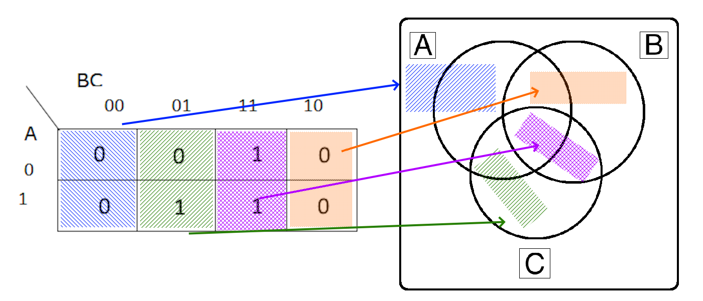
So let’s take a look at example one. And the best way to start this is where the output is actually true. So if we examine this line here, this line and this line, we can see that when B and C are true, output is True. When a and c are true, the output is True, or when all three are true, the output is also true. So a really good way to start is just by coloring in these three facts.
So when B and C are true, that’s this little square here. Then when a and c are true, that’s this little portion of the Venn diagram. And then when a, b, and c are so when all three are true, And that’s this little center part of the diagram. And then all other rows of the truth table are all false or zero. So we’re not going to fill in anything else in the Venn diagram here. So this is the full output of or the full expression represented as a Venn diagram.
So let’s tackle this as a Boolean expression. And so we’ve already talked through parts of what the Boolean expression would actually be. So this can start here with a and c, when a and c are true, the statement is true. So let’s write a and see us as one portion of our Boolean expression. So I’m going to write that using parentheses, and then we have B and C. So I’m going to kind of write this over here, B and C. What that’s the other part of the truth in our Boolean expression, but we can’t just write them side by side, right, we need to join the middle because we also need the center portion. So it’s either a and c are true, or either A and C or B and C. So enter a or operate in between. So if A and C are true, or B and C are true, so that’s this portion right here. So when a and c, or B and C are true, and our expression is true, this will represent our Boolean logical statement. But there are alternative ways to write this. And these aren’t just the only ways another way you could have wrote this would be C, right? Because in all three cases, C is always true. So C, and a or b.
So let’s take a look at what the logic gates look like. So the logic gates and I’m going to write the logic gates for my top statement here. So this one right here, we need to write the left and right hand side of the OR operator first, and the OR operator is going to join these two at the end. The lines here represent the inputs of A, B and C. So I’m going to draw out the input of a because in this case, we have a and c. And those are connected together with the AND operator. And that gives an output and we have the same thing with B and C. So we have B, C, those are both connected together with an AND operator and both of those are joined together using or. So this would be the logic gate for this particular statement here.
Let’s do a bit of a deeper dive into that worked example to explain some of the nuances working with Boolean Logic Expressions, Truth Tables, Venn Diagrams, and the connections between those three. Unfortunately, this is not well explained or covered elsewhere in online resources, but we find that it is really helpful to revisit these concepts here before the end of this module.
This is a lot of conceptual information to digest at once. However, we don’t expect you to become proficient in this right away! This is just meant to be an introduction to the concept of Boolean Logic and Boolean Algebra, which you’ll become more comfortable with over time as you practice your programming skills and take later classes in Computer Science.
For now, we just want to introduce the topic and give you a chance to try it out in the quiz at the end of this module. If you don’t do well on the quiz, don’t sweat it!
This material is handy if you want to review the concepts or get in some practice, but the best way to learn is to just keep doing examples and practicing as you learn to code.
When working with Truth Tables and Venn Diagrams, the key idea to remember is that each line in the Truth Table corresponds to exactly one space in the Venn Diagram.
Each labelled section in the Venn Diagram above corresponds to the variables that are True or 1 in the corresponding Truth Table. We can even draw arrows directly from each line in the Truth Table for Example 1 to the Venn Diagram:
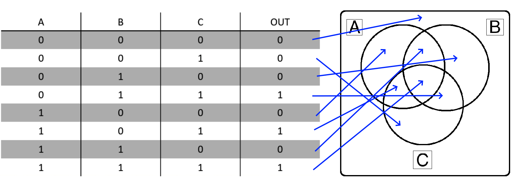
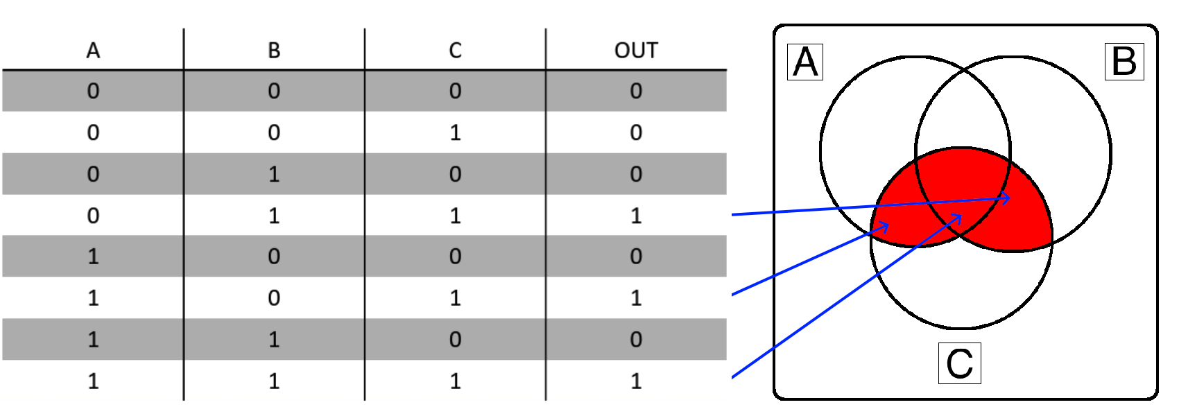
So, if the “OUT” column in the truth table is True or 1, that section of the Venn Diagram becomes shaded and is part of the desired output. Therefore, if you have a Venn Diagram or Truth Table, the conversion between the two is a direct one-to-one connection. Here’s what that looks like for Example 1:
Once we understand either the Truth Table or Venn Diagram for a desired Boolean Logic expression, we can use that information to start building the Boolean Logic expression itself. This can be done in one of three ways:
So, let’s go through these three methods and see how they relate.
Let’s start by directly converting the information in our Truth Table and Venn Diagram to individual Boolean Logic terms. To do this, look at each row in the Venn Diagram where the “OUT” column is 1. Then, for each variable in that row, we either include it in the term directly if it is a True or 1 in the input, or else we include it with a NOT symbol ($\neg$) before the variable if it is a False or 0 in the input. We must include these false variables in our terms, or else we would get different results (i.e. $A \wedge B$ is not the same as $A \wedge B \wedge \neg C$)
So, we would end up with these three terms from our truth table above:
Finally, our full Boolean Expression using these three terms would combine them using the OR ($\vee$) symbol. This is because the “OUT” column in the Truth Table is True or 1 if any one or more of these terms are True. So, our resulting Boolean Expression at this point would be the following:
$$ (\neg A \wedge B \wedge C) \vee (A \wedge \neg B \wedge C) \vee (A \wedge B \wedge C) $$
At this point, we can stop if we don’t care about reducing the expression to simpler terms. So, once again, there is a direct one-to-one translation from either a Truth Table or Venn Diagram to a Boolean Logic expression that is in this form. In fact, this form is known as the Disjunctive Normal Form of a Boolean Logic expression (though it is not the reduced form). A great way to remember this form is that it is an OR of ANDs (the individual terms are all AND operators, and then the terms are combined using OR operators).
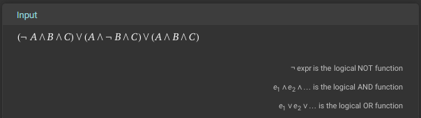
Before we go any further, we can check our work by entering this formula into Wolfram Alpha and checking the Venn Diagram and Truth Table it produces and make sure they match our original setup. While it is possible to enter all of the fancy Boolean Logic symbols into Wolfram Alpha (it does understand them), it is often easiest to just convert them to their English counterparts as shown below:
(NOT A AND B AND C) OR (A AND NOT B AND C) OR (A AND B AND C)You can also click this link to go directly to Wolfram Alpha with this input provided.
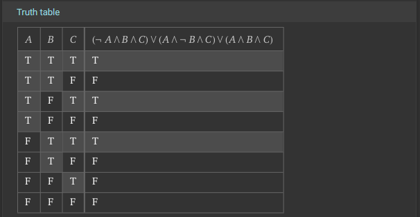
First, we can check that our input is parsed correctly since it matches our Boolean Logic expression at the top:
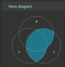
We can also look at the Truth Table and Venn Diagrams further down:
Notice that the Truth Table is ordered a bit differently than what we see above (it is reversed), and the Venn Diagram is rotated a bit, but hopefully it becomes pretty clear that we have a match! So, our translation from the Truth Table to a Boolean Logic Expression is valid!
Once we have a valid Boolean Logic Expression, we can use the laws of Boolean Algebra to reduce it. We cover some of these laws earlier in this chapter, but Wikipedia has a good listing of them as well. We’ll refer to the laws as they are described in Wikipedia as we perform these operations.
First, it is often very helpful to remember that, in many cases, AND ($\wedge$) can be treated similar to multiplication ($\times$), while OR ($\vee$) can be treated like addition ($+$). So, in some fields (such as computer engineering), it is common to rewrite the statement above like this:
$$ (\neg A B C) \vee (A \neg B C) \vee (A B C) $$
This may make some operations more intuitive, especially where we are “factoring out” or “distributing” a term by applying the Distributivity laws. So, we’ll use this modified notation while performing our Boolean Algebra reductions.
Unfortunately, reducing this expression is actually a bit complex, because there is not an obvious starting place. Instead, what we need to do first is duplicate a term by applying the inverse of the Idempotence of $\vee$ law. This law states that $ x \vee x = x $, so we can invert it by replacing any single term $x$ with two instances of the term that are connected with the OR ($\vee$) operator. We’ll do this to the last term in the expression for now:
$$ (\neg A B C) \vee (A \neg B C) \vee (A B C) \vee (A B C) $$
Next, we want to group some similar terms together to make later operations a bit more obvious. So, we’ll apply the Commutativity of $\vee$ law to rearrange the terms, and also use the Associativity of $\vee$ law to group some terms together:
$$ \Big( (\neg A B C) \vee (A B C) \Big) \vee \Big( (A \neg B C)\vee (A B C) \Big) $$
Now we can start to simplify things a bit. In both groups of terms, we notice that they each share the variable $C$, so we can apply the inverse of the Distributivity of $\wedge$ over $\vee$ law to “factor out” that term. Notice that this is very similar to how we can apply a similar law in ordinary algebra:
$$ \Big( C \wedge \big((\neg A B) \vee (A B) \big) \Big) \vee \Big( C \wedge \big( (A \neg B)\vee (A B) \big) \Big) $$
After that, we’ll see that the first pair of remaining terms shares the variable B, while the second pair of terms shares the variable A. So, we can once again apply the Distributivity of $\wedge$ over $\vee$ law to “factor out” those shared terms in each pair:
$$ \Big( C \wedge \big(B \wedge (\neg A \vee A) \big) \Big) \vee \Big( C \wedge \big(A \wedge (\neg B \vee B) \big) \Big) $$
Now we can start to remove some terms. The Complementation 2 law in Wikipedia states that $x \vee \neg x = 1$, which means that we can replace a term and the inverse of that term connected with an OR ($\vee$) operator with the value True or 1. We’ll do this for both $A$ and $B$ terms:
$$ \Big( C \wedge \big(B \wedge 1 \big) \Big) \vee \Big( C \wedge \big(A \wedge 1 \big) \Big) $$
Next, we can use the Identity for $\wedge$ law, which states that $x \wedge 1 = x$, to effectively remove those True or 1 terms from the statement. Again, remember that in regular algebra, we would know that the term $1A$ would be equivalent to just $A$, so if we rewrite $A \wedge 1$ as just $1A$ and then just $A$, it feels very logical!
$$ ( C B ) \vee ( C A ) $$
Finally, if desired, we can apply the Distributivity of $\wedge$ over $\vee$ law one more time to “factor out” the $C$ variable again:
$$ C \wedge (B \vee A) $$
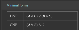
There we go! Both of those reductions are valid minimal forms of the Boolean Logic Expression. Once again, we can go back to Wolfram Alpha to check our work:
In that screenshot, we can see both the minimal Disjunctive Normal Form (DNF) as well as the minimal Conjunctive Normal Form (CNF) for the expression.
Another great way to convert a Truth Table or Venn Diagram into a Boolean Logic Expression is to use a bit of intuition. The video earlier in this chapter showed one way to do this suing the Venn Diagram, but let’s use another method - using a concrete example!
For this example, let’s assume that we have been given the following rules:
We can build a Truth Table using these rules as shown below:
| Friends Over (A) | Sunny Outside (B) | Mom Says Yes (C) | Go Swimming |
|---|---|---|---|
| 0 | 0 | 0 | 0 |
| 0 | 0 | 1 | 0 |
| 0 | 1 | 0 | 0 |
| 0 | 1 | 1 | 1 |
| 1 | 0 | 0 | 0 |
| 1 | 0 | 1 | 1 |
| 1 | 1 | 0 | 0 |
| 1 | 1 | 1 | 1 |
Ahh! Notice that this Truth Table is identical to the Truth Table given in Example 1 shown above! We have created a set of rules that immediately generate the same Boolean Logic Expression that matches our example. It may take a little bit of thinking, and we have to state the rules very clearly, but generally we can always create a set of rules that clearly describe any Truth Table. In practice, we often are starting with a set of rules like this (in our specifications document), and we are trying to build a Boolean Logic Expression that we can use in our code as we implement those specifications in our program.
Now, let’s use a bit of intuition about those rules above to generate a Boolean Logic Expression. If we really want to go swimming, we’ll quickly realize that there are two main things that we need to have:
Look closely at those rules! Just by talking through the scenario, we have created a Boolean Logic expression. Let’s rewrite it:
Mom must say yes
AND(it must be sunny outsideORwe have to have friends over)
If we replace each part with the corresponding variable, we can find the corresponding statement:
$$ C \wedge (B \vee A) $$
A similar way to state the rules might be:
Once again, we can rewrite that a bit to make the Boolean Logic operators more obvious:
(Mom must say yes
ANDit must be sunny outside)OR(Mom must say yesANDwe have to have friends over)
Finally, we can replace those parts with variables to get the corresponding statement:
$$ (C \vee B) \wedge (C \vee A) $$
So, as we can see, applying a bit of intuition to a real-world example that creates the same situation can make it pretty easy to work out a simple Boolean Logic Expression from a Truth Table or Venn Diagram.
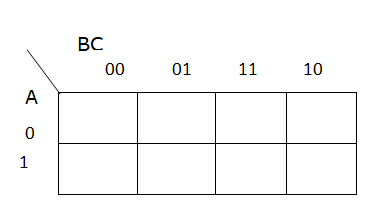
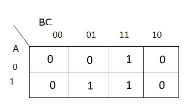
The third method would be to use a Karnaugh Map. We won’t go into this method in too much depth, but we’ll briefly show how it works. There are some great online resources to learn more about applying Karnaugh Maps in this context.
First, we’ll start with a blank 3 variable Karnaugh map. A Karnaugh Map is essentially a different way to structure a truth table by placing similar entries next to each other in a particular way:
Then, we’ll input the desired outputs from the Truth Table in each square of the Karnaugh Map:
Now, we’ll group connected terms. These groups can be either rectangular or square boxes. So, for this Karnaugh Map, there are two groups:
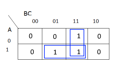
Finally, for each group, we identify the variables that don’t change within that group, and those become our terms. So, for the group in the bottom row, we see that both $A$ and $C$ are the same, but $B$ changes. So, one term we find is $AC$. For the group in the third column, we see that $B$ and $C$ are the same, but $A$ changes, so our other term is $BC$. Then, we combine those two terms together using the OR ($\vee$) operator to get this statement:
$$ (AC) \vee (BC) $$
There we go! That is once again one of our minimal Boolean Logic expressions found earlier.
Once clever things that we might notice is that there is also a one-to-one equivalence between Karnaugh Maps and Venn Diagrams. We know this since there is already a one-to-one equivalence between both of those and the original Truth Tables, so it is an easy assumption to make.
So, we can quickly see the arrangement of items in a Karnaugh Map and how they match up to our Venn Diagrams as shown below:
Notice that the the Venn Diagram has a very similar layout to the Karnaugh Map. This is because both of them are structured in a way for similar entries to be near each other. In fact, each time you cross over a line in a Venn Diagram, only a single variable changes value. The same works for a Karnaugh Map.
So, with a little intuition and an understanding how Karnaugh Maps work, we can perform a similar analysis directly on the Venn Diagram itself.
Why does all of this matter? Well, when we are trying to convert a real-world situation to code, it is often helpful (but not necessary) to be able to reduce our Boolean Logic expressions to simpler terms.
Let’s go back to the concrete example shown above. If we wanted to write a Python program for this, there are a few ways we could build it.
First, here’s what it would look like if we just directly encoded the rules as written:
# bool() returns False if the input is the number 0, otherwise True
# so we have to convert the string to an int first
sunny = bool(int(input("Is it sunny outside? (1 = yes, 0 = no)")))
friends = bool(int(input("Do you have friends over? (1 = yes, 0 = no)")))
mom = bool(int(input("Did Mom say yes? (1 = yes, 0 = no)")))

"""
Rules:
* If Mom says yes and it is sunny outside, we can go swimming even if we don't have friends over.
* If Mom says yes and we have friends over, we can go swimming even if it isn't sunny outside.
* If Mom says yes, we can go swimming if it is sunny outside and we have friends over.
"""

if (mom and sunny and not friends)
  or (mom and friends and not sunny)
  or (mom and friends and sunny):
    print("We can go swimming")
else:
    print("We cannot go swimming")
We could also use if-else statements instead of the or operator to achieve a similar effect:
if mom and sunny and not friends:
  print("We can go swimming")
else if mom and friends and not sunny:
  print("We can go swimming")
else if mom and friends and sunny:
  print("We can go swimming")
else:
  print("We cannot go swimming")
However, in both cases, these programs are more complex than they actually need to be, and it may make things more difficult to debug down the road. So, with a little intuition and the ability to reduce Boolean Logic expressions effectively (and correctly), we can simplify this code quite a bit:
if mom and (sunny or friends):
  print("We can go swimming")
else:
  print("We cannot go swimming")
Hopefully you can see the value in that much simpler program, both in terms of how easy it is to understand and debug, but possibly how much more efficient it is overall since it has fewer comparison to make.
Image Source: https://www.allaboutcircuits.com/textbook/digital/chpt-8/boolean-relationships-on-venn-diagrams/ ↩︎
Image Source: https://www.wolframalpha.com/input?i=%28NOT+A+AND+B+AND+C%29+OR+%28A+AND+NOT+B+AND+C%29+OR+%28A+AND+B+AND+C%29 ↩︎ ↩︎ ↩︎ ↩︎
Image source: https://www.learnelectronicswithme.com/2021/09/karnaugh-map-and-steps-to-solve.html ↩︎
Read Pattern on the Stone, Chapter 2.
“The Pattern on the Stone: The Simple Ideas that Make Computers Work” by W. Daniel Hillis. ISBN 046502596X, newer version is also available and will work fine

In this video, we’re going to take a look at computer programming languages and some of the history that’s behind them. First off, what exactly is a language. Something that we don’t really think about very often though. A language really is just a set of symbols, whether it be gestures, words, sign language, or even Braille, that are used in a uniform fashion to allow people to communicate with one another. We have to take a look at how we as humans can communicate with a physical or inanimate object: a computer. In order for us to tell computers what to do, we had to develop a language that we could use to communicate with it. Here on my slide I have on the left a bunch of different ways on how to say good morning, in various human languages that we use to communicate with with one another. And on the right side here we have a bunch of computer languages that we have. So the first one up here is happens to be Python 2, Python 3, C, Java, JavaScript, and even Rust. And so this is just a small number of different things that we would be able to use to communicate this particular message to our computer. Just likewise, we have a lot of different ways we could say good morning to someone.
Let’s take a look though on where the idea of a computer language actually started to originate from. Ada Lovelace is our first influential woman in computer science that we’ll talk about. She is regarded as one of the first figures in history to truly understand computer programming, possibly only second to Charles Babbage. Ada Lovelace was the daughter of a famous English poet. Lord Byron, who I’m sure you’ve heard about before, but she had very little contact with her dad pretty much at all, and during her childhood, she was pretty much on her own. But during that period due to her father status, she was tutored by some of the greatest mathematicians of that time, including Augustus de Morgan, remember from the Boolean logic lecture, had the De Morgan’s theorem. And so she was already being tutored by some of these great mathematicians who were laying the groundwork and the foundations for what we use in computer science. One of the… one of the greatest quotes from from Charles Babbage, who he was talking about Ada Lovelace with. So, Charles Babbage said that Ada Lovelace was that “Enchantress who was thrown her magical spell around the most abstract of sciences and has grasped it with a force few masculine intellects could ever have exerted over it.” So this is a really big compliment from Charles Babbage, who was pretty much the pioneer in computer science at the time.
Ada Lovelace spent a lot of time visiting Charles Babbage and she was so intrigued by his Difference Engine that he had in his house, the prototype that he had made. But her goal in visiting with Charles Babbage so much is that she started to translate his work into English so she could bring it back to England, and explain how it worked and why it was so important and revolutionary. And to assist with that she included a set of notes with her own descriptions of the design of his Difference and Analytical Engines and how they actually worked and when completed her notes are actually longer than Charles Babbage’s memoir. She has so she had a very deep understanding on how Charles Babbage’s machines actually work.
What makes Ada Lovelace so unique in the history of computing is Section G here in her notes. in that section she describes in complete and utter detail how you would use Babbage’s analytical engine to calculate a sequence of numbers called the Bernoulli numbers. You’re probably also familiar with. But while it appears to be written in English, it’s actually designed in a way that can be directly used by the Analytical Engine. So, in a way, you could say that it is in a language that the analytical engine would understand. And in doing so, she wrote the first computer program, which is simply, right, a series of steps specifically designed in such a way that could be easily ran on a computer.
There is some debate as to whether or not she wrote some of the programs she was previously attributed to. But there’s little doubt in the fact that she would be capable of doing so. In fact, she was one of the few people who saw the true potential of what Babbage had actually created. And she’d once remarked that under the correct circumstances, it could be used to create music. So the Analytical Engine she was talking about here. And that’s really quite extraordinary, something that Babbage probably hadn’t thought of at the time. But if you are a musicphile at all, music, right is just simple mathematics. And so if you have a machine that can compute mathematical values, why wouldn’t it be used to create music? So all told, Ada Lovelace is really truly a very important person in the history of computing science. And she’s widely regarded as the world’s first true computer programmer. And as a as another bonus side note here, she’s actually credited with discovering the first bug in a computer program as well. A bug. In fact that was found in a program that was written by Charles Babbage.
Our next famous woman in computer science that we’ll be talking about is Rear Admiral Grace Hopper. Grace Hopper enlisted in the Navy and worked on the Harvard Mark I computer, as well as the UNIVAC, a successor to the ENIAC, and we’ll talk about the UNIVAC and ENIAC computers in another lecture. So grace also developed a programming language called FlowMatic which was later adapted into a language called COBOL, which is still somewhat used today. COBOL is traditionally a language that was used very heavily in the financial industry, because it was used to generate a lot of financial reports. You don’t see it a whole lot now, you may see it used occasionally at places like banks, or accounting firms and things like that, but it’s not very widely used anymore.
But beyond that, she was a truly a pioneer and out of the box thinker for her entire life. And as you’ll see in the following videos, Grace Hopper is a pretty sassy lady but a pioneer in modern computing. She was also pretty famous for her description of a nanosecond in the Dave letterman show, which you’ll see here in just a little bit. Another thing here every year, there is a Grace Hopper conference to celebrate diversity and inclusion and women in computing. And so there’s actually scholarships available for students if you would like to attend this conference. And it’s something that I would highly recommend if you ever get the chance, it is truly a great experience to actually participate in.
YouTube VideoDue to the privacy settings, we were not able to embed the following video directly.
Discussion of a nanosecond starts at 4:17
YouTube VideoThe next influential woman in computer science that we’ll talk about here is Margaret Hamilton. Margaret was the director of software engineering at MIT’s instrumentation lab. Margaret Hamilton was also known as the, essentially the creator of the field of software engineering, essentially. But the reason why she is credited for software engineering is that she was responsible for a team that developed onboard flight software for the Apollo space program. During this timeframe, her program actually prevented a mission abort during the Apollo 11 moon landing, which is kind of crazy cool to think about right.
In this picture here is, she’s actually standing next to the output of one of the programs that they had actually made. In the video here you’ll see that, you know, programming at this time was completely by the seat of your pants, right? There was no really step by step procedure or best practice of programming pretty much anything. And so the idea that NASA trusted this group of engineers to create the flight software for the Apollo space program was really kind of crazy to think about. And so if you had actually messed up, right, the output of your program would just be you know, feet high instead of just a few pages long, which is this famous picture with Margaret Hamilton here in the slide.
So what really is programming? Right? We’ve talked about a lot of famous women in computer science so far, that have been very influential; the first computer programmer Ada Lovelace, the queen of software Grace Hopper, and Margaret Hamilton, who really pioneered the idea of software engineering, best practices with computer programming. But, what does that really actually entail? Well, programming itself, right computer programming, is simply the act of designing, writing, debugging and maintaining the source code of a computer program.
Let’s imagine that we’re writing a program, a very simple program, that takes input from the user, and then prints out a result that is divided by 61. So the user inputs a number and then we divide it by 61 and output it. So what would that program actually look like? Well, in Scratch, right, it would look something like this. This programming language is very English like, right? It’s a block based programming language that is designed to teach young kids, even up through middle school on basically how to program. And it makes it a lot easier for humans to understand. Because even if I showed this to my grandma, she could probably deduce kind of what’s going on here. Ask for a number and wait, and then divide whatever the answer to that question was by 61. And stop, right? Simple enough. So, very easy for a human to understand.
But do you really think that a computer is able to understand this language? Probably not, right? My computer has no idea what the idea of a block is, right? Computers really only only care about ones and zeros. That’s it. So how do we get from a block down to something a computer can actually understand? So that’s really going to highlight our language hierarchy here. So our high level languages, so the stuff that humans can understand, so stuff that we can understand is what we pretty much deal with on a daily basis as computer scientists. But, then we can kind of go down our stack right into the assembly, machine code, and then down on the hardware, where the actual physical hardware could actually interpret what we’re trying to talk about. But first off, let’s take a look at more high level languages.
So we’ve already showcased Scratch, which is a very human readable. But here is a program written in C or C++. And we’re now starting to get into some stuff that is not so human readable. This in general requires a little bit of training in order to understand, right? Just like if you don’t know Spanish or French, if you are trying to read something in that, in that different language, you need a little bit of training to figure out what was going on. So we have a lot of extra syntax here like printf, right? What does that mean? What is a float? If I, if this is the first time ever reading a programming language, I’d have no idea what some of these things actually are. But again, right, this is the same program: input a number divide it by 61. And then output that result.
Same thing goes with Java, right? As you can see here, we have a lot more, a lot more fluff, right. So we have a bunch of import statements up here. We have we now have to have a class and we have to have a public static void main string args, whatever the heck that’s supposed to mean, right? And even beginner Java programmers aren’t even introduced to this concept until once you get deeper into that particular course, What’s a scanner? What are we scanning? I don’t know. So again, right requires a little bit of extra training and Java, with it being an object oriented programming language, adds a lot more fluff and syntax and wrapping to our program just for a simple program like this in order for it to work.
And C# isn’t much better. C# is essentially Microsoft’s flavor of Java, but does the same thing right: inputs a number, divides by 61 and outputs it. I would argue that this code here is a little bit easier to understand. But again, right, we have a bunch of extra fluff here that you know, start from scratch is a little bit more difficult to understand without a little extra training.
Now Python, like Scratch, is generally touted very human readable. So it doesn’t have all of that extra fluff, right? We have no class, or namespace or inputs, or sorry, imports to define here. We just take input, and then convert it to an int, store it and then print out the result, right? Simple enough. So all of this extra fluff that we had here, in C#, I’ve reduced all of this down to two lines in Python. That’s why Python is traditionally used as a scientific language because it’s a lot more accessible to non-computer scientists.
But again, right, there’s tons of different programming languages out there and they all have their purpose. They all have their place. Some more human readable than others, right? We’ve talked about COBOL already right with Grace Hopper, Pascal, Visual Basic Perl, fortran which is an old one as well. Basic is another older programming language. There’s way too many of them to list here. But the point is we have a lot of different languages with the various different purposes, but all of them with a trained computer programmer, could use them to communicate their particular idea or task or whatever they’re trying to do to the computer. But again, right, all of those languages can’t be understood by the computer directly.
The majority of those languages will have then a compiler associated with them. And compiler or assembly is typically a language that is assembly language is typically still readable by humans, but is much closer to the language a computer would actually understand. And assembly language requires much more training to actually understand what’s going on. And so to go from a high level language to assembly language, we’ll use a program called a compiler, which in its entire purpose is to act as a translator. So the language that we use to write our program and like Python, or Java, let’s say, is then compiled and translated down into an assembly language, which is closer to what the computer can understand. Here’s our C program, the assembly language that’s associated with that after it’s been compiled. This particular part is simply, right, taking a number and dividing it by 61. And this is, this is a heck of a lot more complex, isn’t it? Right? You will eventually, or if you, if you take some of our upper level computer science courses, you will learn how to translate all of this and understand what’s going on here. But the majority of computer scientists aren’t going to need to understand assembly language unless you’re dealing more with things at the operating system level or hardware level and things like that, or even cybersecurity if you’re into cybersecurity, being able to understand some assembly is quite useful. Not directly interpretable by your hardware quite yet.
Once we have our assembly language that is going to be then fed into the assembler, the assembler is going to take the assembly language and convert it into machine code, which is then directly read by your computer. The assembly and things like that. Some of this will actually depend on the operating system, the architecture and things like that, that you’re actually running on your computer. While the high level language is uniform, mostly across all machines, the assembly code is not. Likewise, machine language is very specific to the machine that it’s being built for. So, machine language is just simply a set of binary code, all ones and zeros, that tell the computer exactly what to do. And so here’s the machine code for the assembly language that we just saw previously. Theoretically, right? You could translate all these ones and zeros back into the original program. But that’s pretty difficult to do, right? It requires a significant amount of training to be able to try to translate these ones and zeros back into what it was originally.
And so now we’re getting into code that can be interpreted directly by your machines, hardware. Your hardware, really all it cares about is current or no current, right? Electricity is on or the electricity is off. And so this simply refers to the structure of chips and circuits that your computer is made of. And we’ll talk more about that in another lecture. But, and the gist of it here, right, we’re feeding all of our ones and zeros into each of the inputs of our hardware, which is taking those ones and zeros, doing some sort of calculation and outputting the result back to your computer.
But overall, right this is kind of the big picture of computer programming, right? We go from a high level language, where we have things like Python, C, C#, Java, JavaScript, all of those languages that you would normally program in, as a, as a software engineer. And those languages are then compiled or taken by a compiler and compiled into assembly language, which is more machine specific, right, depending on operating system, Mac, Apple, Linux, that sort of thing. 64 bit versus 32 bit processor, lots of different things that go into that particular compilation. But that assembly language is then assembled, taken by the assembler and then converted into machine language which is just the ones and zeros that your hardware is going to interpret
Read Pattern on the Stone, Chapter 3.
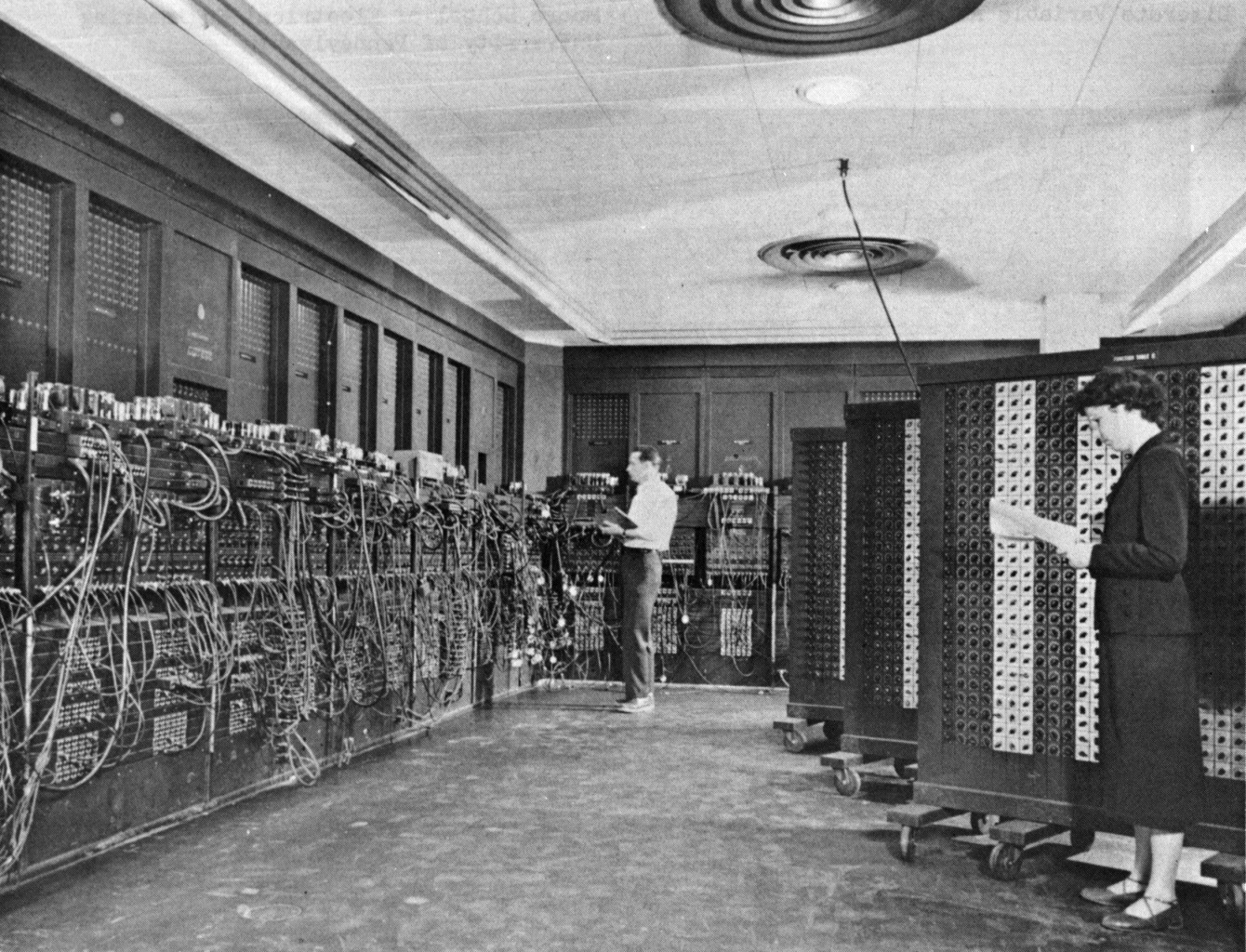
Welcome back, everyone. In today’s video, we’re going to be talking about universal computers. Now to pretty much pick up where we left off a while ago when we were talking about Boolean logic, Claude Shannon had just proposed a way to take electrical circuits and represent any Boolean logical statement with them. And so this was a huge turning point in the history of computer science. But how did we make the leap from Boolean logic on electrical circuits to the modern computers that we have today, and we’ll talk a little bit about that gap here today, but there will still be some missing parts that we’ll talk about later. But this brings us to Herman Hollerith, who at the time was a United States Census office employee, and he was tasked with coming up with a better way to calculate the census result. Because at the time, calculating the US census was incredibly slow. The 1880 census alone took eight years to tabulate, which really kind of defeats the purpose of a census, right? If you only know how many people you have in your country, eight years after the fact, the census was actually taken.
And so 10 years later, Herman had actually implemented a new system. And so in 1890, when he tabulated the US Census, then it only took one year to complete versus the eight years from the 1880 census. And this is even taking into account the 30% increase in population over that decade, which is pretty impressive, to say the least. So how did he do it? Well, just as Joseph Marie Jacquard had discovered, punch cards are really great way to organize and calculate information, particularly when you want that information to be read and used by machines. And so Hollerith was inspired by this fact. But really, actually, he was inspired by the way railroad conductors would actually use punch cards to track the gender and age and so forth from people buying tickets for the railroad. So not only did Herman Hollerith develop a new punch card in order to track US Census data, he also developed a machine to actually read it.
So this is an example of a Hollerith tabulating machine that was used in the 1890 census. So this machine could read the card and tabulate all of the information that was on them, and was also advanced enough to actually infer other facts and keep track of things like the number of married men and women. And depending on the data on the card, there is a compartment down you can kind of see towards the bottom right hand corner there. That was a storage box, for the cards and so depending on what kind of data was actually on the cards, a compartment in this storage box would open. So the operator that was using the machine could take the card from the machine and put it in the corresponding box. So essentially right it was auto sorting all of the census data, which was also pretty cool. But Hollerith continued to improve his designs and created several upgraded machines that could tabulate all sorts of data, not just census and donation, he would go on to create his own company, the Tabulating Machine Company, and a couple decades later, his company would join several under under a new name the Computing Tabulating Recording Company. But this was eventually renamed to be something else, the International Business Machines company, right. And many of you all know this company as IBM. Pretty cool, right?
This is something that I learned when coming to computer science, I had no idea how IBM got their start, but tabulating machines is pretty much where they come from. Now, this particular image from this slide is from the US Social Security Administration in 1936. This shows several IBM tabulating and sorting machines in use. And so they use these for all sorts of things as time progressed, and each one was able to keep track of all sorts of different kinds of information. One example could be tracking the sales of a particular person or company for the purpose of billing, right, or tabulating sales, and inside of a convenience store or something like that. Does all sorts of things, right. So things that were traditionally done on pen and paper or pencil and paper, and prone to a lot of human error. We could feed these punch cards through these machines and they would auto tabulate everything. For us, and they were pretty popular all the way through the 50s and 60s, until the computer started to take over really, but this pretty long time, right? About 30 years or so, for these tabulating machines, as they kind of took their grip. But we’ll talk a little bit here in just a second about the actual first computers that we actually had in the United States. But just as a quick little fun fact, we’ve talked briefly in a previous video How pretty much took a country torn by war before we actually started, or the world torn by war, really. Before we started to get a lot of advancements in computing technology. IBM was actually involved with selling these tabulating machines to the Nazi Party in Germany and may have inadvertently aided their attempts to catalog and later persecute the Jews. During the Holocaust, so a little bit of dark history behind IBM and their tabulating machines.
But anyways, let’s talk about the some of the early major computers that we actually had in the US. So, first and foremost, the mark one, the mark one that was really important because we started to see a shift from pure mechanical computers or computers like tabulating machines to something that was a little bit more flexible, a little bit more powerful, as far as what type calculations that could be done. But the mark one was an electromechanical computer, and it was the largest of its type ever built. And its main purpose was actually to aid in the calculating ballistics tables that were needed by the gunners to accurately aim and fire weapons that were being developed for the war because to try to stay ahead, the US was developing weapon at an alarming rate. And the time it would take about 20 hours for a skilled mathematician to analyze a single 60 second trajectory shot. This is way too slow at the pace that weapons are actually being developed. And so the mark one was completed 13 years after it was commissioned in 1944. And proved to be pretty useful, right. So this is also remember back with Grace Hopper when we talked about her. This was the computer that she was commissioned to work on by the US Navy. So then let’s chat about the kind of the next step up right. So the mark one was an electro mechanical computer, which had tons of parts, right. Five tons of computer if you can imagine that. And one little But the fun fact that I always like to emphasize here is that the mark one had five horsepower. Right? So it actually had an engine their in order to run it. So if you can kind of imagine having a laptop that had an engine in order for it to actually work kind of crazy to think about that your computer has horsepower.
But we did take a big leap forward after the mark one was completed. So in 1943, the US Army and the University of Pennsylvania began working on a project that would be the successor to the mark one called the electrical numerical integrator and calculator or any ENIAC right. Scientists like acronyms, and sometimes they’re pretty good. Sometimes they’re not so great. But when the ENIAC was completed in 1946, it turned out to be about 1000 times faster than the mark one. But the ENIAC was so revolutionary. because it was the first all electric programmable computer that was truly general purpose. And we’ll talk about that here in just a little bit. But remember how we were talking about the Difference Engine that Charles Babbage created that was truly are the Difference Engine number two in the analytical engine that were truly general purpose computers, right. And so now we have the first all electric computer compared to the mark one, which still had a lot of the mechanical parts right had five horsepower. But the ENIAC ran almost continuously from 1946 to 1955. So had a pretty good long, long term operation here. Again, right had an insane number of parts right over 17,000 vacuum tubes that were used to run at 70,000 resistors, 10,000, capacitors and over 5 million hand soldered joints. If you have a hard time trying to figure out what’s wrong with your computer Now, imagine trying to debug and fix a computer that had so many different moving parts or so many different hand soldered parts is really kind of crazy to think about. But we’ll bring up the neck and the mark one and another lecture as well.
But I do kind of want to highlight a really big important part during this time frame, right? During the mark one and the ENIAC because remember, this is during World War Two, where a lot of the men were overseas fighting the war. And so a really far less known fact in computer science right? Early computer scientists were all women. So in the early days of computer science, the mark one ENIAC the majority of these machines and computers were being serviced, programmed and ran by women during the war. There’s this awesome documentary called the Top Secret Rosies, I would highly recommend watching the entire documentary. I’m sure you could probably find it streaming online somewhere. But this particular clip that I will show here in just a little bit, is just kind of a summary of the role of these women played during World War Two
So what really is a universal computer? We’ve thrown that term around a little bit. We’ve also talked about what it means to be a truly general purpose computer or reprogrammable computer compared to a fixed program computer like what the original Difference Engine was. So, this is what made the ENIAC so unique as well as the mark one, although to a lesser extent. is the fact that they are considered the world’s first true universal computers. So what do you think it means to be called a universal computer? Well, a universal computer can simulate any real world computer given infinite time and infinite memory. So if you imagine taking your cell phone or even something as small as like the little Raspberry Pi or a smartwatch. And if it was truly a universal computer, if you gave it enough time and enough memory, it could pretty much do anything any other computer could do. So compare that to some supercomputer right like Beocat that we have in the computer science department here at K-State. Right, a universal computer can do anything that Beocat can do, given enough time and give it given enough space.
So this brings us to Alan Turing. Now, Alan Turing was one of the first people to come up with this idea of a truly universal computer. Now, in 1936, he proposed this idea of an imaginary computer, and this imaginary computer was so simple, it was like it couldn’t do anything right. And actually Alan Turing was mocked quite extensive. Simply for coming up with this idea because people thought it was just crazy that it wouldn’t work. But now we know this imaginary computer to be known as the Turing machine. But in reality, this Turing machine, this simple machine that he kind of came up with, was able to do and calculate any value that could be done by any other computer, even though it was crazy simple. So let’s take a look at an example of what a Turing machine might look like right because it was an imaginary computer an imaginary machine.
So a Turing machine itself consisted of a an infinitely long tape, and this tape is divided. It has individual squares on it, just kind of like a roll of film wood and a classic non digital camera anyways, but each individual square you could would be either a one or a zero or it could be blank if it hadn’t had any data written to it yet. Now the machine actually works by moving back and forth along the tape and reading and writing ones and zeros depending on the value that actually reads out from the tape. But how does it actually know where to go? Well, if you can see here in the picture, there’s this little controller in the system as well.
Now this controller would have had a program pre loaded onto it. And so we could write this program using these commands here and it’s relatively simple, right? We have eight different commands right, move left, and move right, right one, right, zero, read. So the read is if this square is zero, or if this square is one, go to Step x in the program. And then we also have just a straight, go to Step whatever, and stop. So the program itself right could only consist of these eight steps and here in another video, we’ll take a look at an example of these eight steps in action. But it’s really important to emphasize how cool this actually is right? The simplicity of these eight basic steps represent a universal computer. And this universal computer right is just a can accomplish just as much as something a supercomputer could do like Beocat. So, given enough time, and memory, a Turring machine with these eight basic steps, and only reading and writing ones and zeros could accomplish any problem.
Hello everyone in this video we’re going to take a look at a detailed example on how a Turing machine may actually perform a common operation that we would do with a regular program. Remember that our Turing machine has eight simple instructions that it can execute using the control arm or the the reader that the machine or the program is actually loaded on. But it can simply move left or right one, it can write ones and zeros and it can also read and also jump around in the program as well. So these eight simple steps remember represent a truly universal computer given enough time, and given enough memory, it can perform any operation any other real world computer could actually do. So here’s an example of a basic program on our Turing machine. So our reader or the Turing machine itself would be preloaded with this program. In this situation, we’re going to assume that we start with two elements or two items or two pieces of data on our tape. And these items, remember, all we’re dealing with here are ones and zeros, nothing else.
So we’ll start with two binary digits on our tape. And then the program has just a finite number of steps here, so steps one through 11. And you can see here we jump around a little bit. For example, in step one, if we read a one on the tape, then we’re going to jump to step number five in our program. So the go to number five isn’t a step to number five in our tape, it is go to number five in our actual programs, line five in our program. For this example we’re actually going to do here is we’re going to step through our program overall and try to figure out what kind of operation it’s actually trying to perform is just looking at this straight up. It’s kind of hard to tell what we’re actually trying to accomplish or what the Turing machine is actually trying to accomplish.
So let’s work out this example here. So since we only start with two binary digits on our tape, that really means we only have four possible combinations in total, right, we only have two binary digits to the power of two is four. So this is the number of combinations of those two digits that we might actually have. So let’s go ahead and write to these different combinations out here. We have 0 0. We have 0 1, 1 0, and finally, 1 1. So I’m going to go ahead and label these different cases here. So we can kind of keep track of them a little bit better. So this is case A, B, C, and let’s call this one over here. D Now this is a little bit different than how we would normally actually read things. In this case for my Turing machine, I’m going to read my inputs or start my inputs from left to right. So if we start out our program here at step number one, I’m going to go ahead and just work on example A here first or this data A here first, to our head, our reader, our Turing machine, starts looking at the first square out. Step number one, and our program says if one, go to Step Five. Now, the data that we have here is actually just a zero, so we’re not going to jump to step five. So we’ll actually just continue on and go to step number two.
Now notice that my head over here, or where my Turing machine is actually reading from does not actually move until I tell it to. Now step two does tell us to move left. And so you can either imagine this as the head moving left, or the tape moving in the opposite direction. And so what that actually causes us to do is we’re going to no longer be in that spot are going to move on to this square. So then let’s continue on to our next step here. So we already move left and so we’ll keep on executing our program sequentially. So at step number three, we have if 0, go to step nine. So if 0 is true. So we were reading a 0 here, I’m going to jump from step three, all the way down to step nine. Step nine, says move left. So we’re going to move our tape over here to this empty square. And then we’re going to go down to the next step, step 10. Step 10 says write a 0. So my, machine is going to write a zero here. And then we’ll continue on to our next step of our program, and our Turing machine stops. So our output here, this is our output, what our machine actually wrote out as a result of running our program, given the starting data.
Let’s continue on. Let’s go and look at another example here. So if we look at our second data set here, we are going to again, start at our first position here. And start out at number one on our slides over here or on our on our list over here. So if one, go to Step five, and so this indeed is a one. So that is that is good. And so we’re going to skip steps two, three and four, and go down to step five. Step five tells us to move left. So I’m going to move left here. And that’s step five. And then step six says move left again, though, we’re going to stop that, move our Turing machine, head over one. Step seven, tells us to write a one. And then we go down to step eight, and that says, Stop. So this was the result of doing our data B over here. This particular example. So our first one, we read two zeros and output at zero. In this case, we read a one. And then we, we moved over to zero, but we didn’t actually read this one, right? Remember, we didn’t actually read the second data piece, we only read our first piece of information, and then we skipped over zero and then wrote a one in our empty spot. So let’s do more examples.
You still have C, and D to go. So again, we’re going to start out over here at our first piece of information. Step one, right, step one, go to Step five, so that’s not true. So we’re going to jump down here to step number two. Step number two says move left. So we’re going to move left one Then continue on to Step three. That three says if zero go to nine, well, that’s not true because we’re at a, our, our current carrying machine tape square has a one on it, it will go down to step four, which says if one go to Step six, which is true, though, that is true. So we’re going to go to step number six, then that tells us to move left, go on to Step seven. Step seven, tells us to write a one and then the top. So very similar case as what we had for be here where we read a one, skip to zero, wrote one. Here, we wrote as we read a zero, move left, write a one and then output it. And then finally, just to kind of put this last the this dataset to rest here, let’s check out D. This will be the final indicator for what kind of operation that we’re actually trying to showcase here.
So just like what we’ve done before, we’re going to start out at our first square on our Turing machine tape. And then of course, start out at our first step in our program. So if one go to step number five, so our square that we’re at is indeed a one. So we’re going to skip all the way down here to step number five. Step number five, says, move left though, I’m going to move the machine over one. Step six says move left. I’m going to move over one again. Then, step seven says write a one. Oh, well, let’s try to one here and that square and then Stop. So that’s pretty much it for our particular Turing machine example, for this particular program, we’ve covered all of the different combinations of data that we possibly could have on our tape for this particular program.
Now, what kind of operation Could you imagine would actually be represented here? Oh, really, the hint is how the program or what the program outputted when we actually read our ones and zeros out, the only time that we actually out voted a, we wrote out a zero was when both of our inputs here were heroes. Right? So when we had two zeros, so remember, zero meaning false and one meaning true in binary, so, zero and zero is zero. So starting to look like a Boolean operator. So if we come down and look at B. So we have for a we had zero whatever the operator is zero, and that equals zero. So for B, we had, we had one , zero, which is one, for C, we had zero, one. And that was a one. And then for D, we had one, one, which is one. Now, what is the binary or not that sorry, not the binary, the Boolean operator that unifies all of these statements. Well, it’s not AND right, because if and was the operator here, this would output false ,right, so one and zero would be zero not one, or true and false is false. So it’s not that and it’s not the exclusive OR either because exclusive OR would have made D equal false. So one XOR one would be to write because XOR is one or the other, but not both. So really the only to the left, the only Boolean operator that takes two operands right, left hand and right hand side, the only one that we have left is OR so if we put OR here, zero or zero is 0, 1, OR zero is one, zero OR one is one, and one OR one is one. So this Turing machine is simply OR Or you can, if you remember from the Boolean algebra, right, it’s For our examples that we’re going to be doing in class other examples that we’ll be doing in class will have you try your shot at trying to analyze a Turing machine program to figure out what kind of Boolean operator it may be, or even making your own Boolean operator program as as a Turing machine.
Unfortunately, with all the computers that we’ve talked about so far, they don’t really look like the computers that we have today, right? These machines took up entire, literally entire rooms and weighed tons and had millions upon millions of different individual parts. And so how did we get from a giant computer that takes up our room to a computer that fits on your wrist? And so the last piece of that puzzle comes to us from John Von Neumann, and some call him the last of the great mathematicians. And his accomplishments are truly outstanding, although you may hear some feedback against calling him the last of the great mathematician. But where does Von Neumann actually come into play with computer science history?
Well Von Nueman is credited for the Von Neumann architecture. And now really the Von Neumann architecture really sets the stage for modern computing of the way our current computers right now are structured overall. So the Von Neumann architecture contains a few primary parts here, we have the control unit, which is responsible for following and sorting instructions, the arithmetic logic unit, which handles all the calculations, we also have a device that is used for storing memory. And we also have some possible way of inputting and outputting content, right. So we can input whether whatever it may be, that could be a keyboard, that could be a program that we give the computer and we also have some form of output, whether it be a screen, a video, whatever it actually may be. So we think a little bit farther back when we talked about what a computer should be able to do, right? A computer should be able to store stuff It should be able to calculate things, it should be able to be programmable, right, we should be able to accept variable input, and we should be able to output, right. And this pretty much accomplishes all of those things.
And really, nothing has changed since the 1940s, when the Von Neumann architecture was designed and published. Now, I’m personally actually really interested to see how computing continues to evolve. And when we talk about hardware, you may see a few things about you know how some of this has changed a little bit. But the core idea of how our computing devices are now even modern day desktops, laptops and things like that are pretty much the same. There are some minor tweaks and reformulations of this idea, but nothing has drastically changed since then. So really, it’s going to be interesting to see what the future holds. With the structure of competing, right, are we going to, you know, what’s DNA computing going to do? Is that going to change the structure of our bond? Is that going to change or break the Von Neumann architecture? Are we going to gravitate to something completely entirely different? I’m not sure but it’ll be really exciting to see what happens in the next few years.
Read Pattern on the Stone, Chapter 4.

In this module, we’re going to learn about algorithms. But before we can discuss algorithms, let’s take a look at something that you might be very familiar with and see how it actually relates to the idea of an algorithm. For example, we can ask ourselves, how do you shuffle cards? It’s something that is really hard to describe. But once you see it, and you can observe other people doing it, it’s pretty easy to understand what’s going on. But to really know how to shuffle cards, we have to ask ourselves, what items do we need? What tools do we need? Do we need any skills and do any prior knowledge for example, we need to know what a deck of cards is, we need to know what shuffling means we need to know how to manipulate the cards in such a way that they will become shuffled. And of course, even then, the terminology we use is still very difficult. In years past, when I’ve asked students how to shuffle cards, they’ll usually tell me something like cut the deck and then hold them up like this and then ruffle the cards together and it will work. But of course, if you don’t know that cutting the deck means separating the top half from the bottom half and not taking a pair of scissors and cutting them in half. That might be really hard to understand.
And so in this module, we’re going to talk about algorithms and specifically, why it’s very important when you’re writing an algorithm for a computer to be very specific and very explicit about the steps you want it to take. Otherwise, it will not do exactly what you want it to do. So first, we can talk about where the word algorithm comes from. And the word algorithm comes from the name Al - Khwarizmi, which is a shorter version of the name of Abu Abdallah Muhammad ibn Musa al-Khwarizmi . He was a mathematician in the 9th century A.D in Persia. And one of the things he did is he wrote a lot of books on contemporary mathematics. And one of his books was very unique because it included a set of steps to solve some common mathematical problems. And those steps form the basis of what we now call an algorithm for solving those problems. And so in the next video after this, we’re going to see a little bit more about The history of Al-Khwarizmi and why he is so important and so interesting in the field of computer science.
So what is an algorithm in computer science? A good definition for an algorithm is a finite list of specific instructions for carrying out a procedure or solving a problem. If you think about it, every computer program we write consists of many different algorithms. Because as we’ve learned, writing a computer program is exactly that. It’s giving the computer a list of very specific instructions that we’d like it to carry out so that it can perform a task or solve a problem for us. So let’s look at an example of what an algorithm looks like. One of the most common algorithms used today is Euclid’s algorithm. Euclid was a Greek mathematician from 300 B.C, and his algorithm was developed to find the greatest common divisor of two numbers. That greatest common divisor if you studied algebra is used to reduce fractions. And even today in our computers and calculators. We use a modified version of this algorithm to do exactly this task. It really is one of the most efficient ways to To do this, so let’s explore what Euclid’s algorithm looks like and take a look at an example.
So Euclid’s algorithm consists of four simple steps. The first step is you start with two numbers labeled A and B. In the second step, if either of those numbers is zero, the answer is obviously the other number. However, if neither of those numbers is zero, we’ll take the smaller number, and we’ll subtract it from the larger number. Then we’ll repeat those steps two through four until an answer is found. So what we will repeatedly do is take the larger number, subtract the smaller number from it, which will make the larger number smaller. And we repeat that process over and over and over again until we find an answer. So let’s take a look at an example and see how this works. So let’s look at an example of finding the greatest common divisor of 1071 and 462. So we’ll start with our two numbers 1071 and 462. Now, we know that we need to label these numbers A and B. So I’m going to label 1071 as A, and I’m going to label 462. as B. In the algorithm, we see the first step is to see if either of these numbers are zero. So looking at these numbers, 1071 and 462, neither of them zero, so we can move on to Step three, which is subtracting the smaller number from the larger one. So we’ll replace a with 1071. And we’ll subtract 462 from that. And that will give us the result 609. So now our numbers are 609 and 462. Once again, we start over at step two, we see that neither of these numbers are zero. So we do the same thing again, A is still our larger number. So we’ll do 609 minus 462 and we will get 147 and B will still be 462.
So we can keep repeating this process. Now B is the smallest number, so we’ll do 462 minus 147 and we will get 315. Now we have 315, 315 is again, let the larger number, so we’ll subtract 147 again, and this time we will get 168. And 168 is greater than 147 again, so we will subtract 147. And we will get, I’ll go over here to a second column, we will get 21. So now our numbers are 147 and 21. So once again, we need to subtract 21 from 147. And I’ll just kind of do this quickly. We’ll get 126 then we’ll get 105. Then we’ll get 84, 63, 42. then we will get 21. And we’ll notice that here, they’re both the same number. So if we subtract that again, we’ll get zero. And so now that we have zero as one of our numbers, we know that the greatest common divisor of 1071 and 462 is 21. This slide shows that example worked out a little bit clearer so you can follow it. If you’re interested in the greatest common divisor algorithm written by Euclid, I encourage you to pick just two random numbers and see if you can perform this same process. It should work on any two random numbers you pick, but we were very careful in picking 1071 and 462. So we got a larger number as the greatest common divisor. Don’t be surprised if you find out the answer is something small like two or three. That is pretty common as well.
In these next couple of videos, we’re going to introduce the concept of sorting algorithms. Sorting algorithms are used when we want to arrange sets of data in order either from smallest to largest or largest to smallest in our computer programs. As it turns out, there are many different ways that we can sort our data using different algorithms. And each of those algorithms have unique characteristics that make them suitable for certain types of data in certain situations. To really explore sorting algorithms, we’re going to perform these sorting algorithms using a deck of cards. So if you have access to a deck of cards, I encourage you to go find one and take out maybe 8 or 10 cards in a certain order. I have the cards Ace through 10 here, and you’ll be able to follow along with our examples on these next few videos. Before we get started, I’d like you to take the cards that you have selected, shuffled them up a little bit, and then lay them out in front of you and try and sort them in order from smallest to largest. And while you do that, I’d like you to think in your mind about the exact steps that you’re following. For example, are you looking for the smallest card and moving it to one side, or looking for the largest card and moving it to the other side? Or are you trying to arrange little bits of it at a time and slowly put those pieces together until they form the full sort of deck of cards, it might be really interesting to see how the method that you naturally follow matches up with one of these algorithms that we’re going to take a look at. In particular, we’re going to look at four different sorting algorithms, insertion Sort, bubble sort, merge, sort, and quicksort.
The first example is insertion sort. In insertion sort, there’s basically three steps. And you can see in this graphic up above how they work. First, we’ll choose an element from our array, and we’ll place it in the correct place in our destination. So we go through we take the card, we put it where we want, and we repeat until our array is empty and we have completely sorted the cards. So let’s take a look at it. An example of how to do that using a deck of cards. Let’s take a look at how to use a deck of cards to simulate insertion sorts. Here I’ve selected 10 cards out of a deck of cards, and I’ve arranged them in a random order. If you want to follow along at home, feel free to grab either a suit out of a deck of cards, or you can grab just 10 cards in numerical order. In this case, I’m using the ace is one at the low end of the scale. So to do insertion sort, all we have to do is take each value out of our initial array and place it where it would go in the final array. So the first value we’ll have is a nine and we know that that needs to go in the 9th position here. Then we have the 4 we know that the 4 has to go before the 9. Now we have the 8 and we know that the 8 goes between the 4 and the 9. We get a three. It needs to go before the 4. We get to it goes before the three now we get a 5 the 5, does not go here does not go here, but it goes after the four. So we’ll move all of these down and make room for the 5. The ace, of course goes here at the beginning, the 10, we look through, and we see that it goes all the way at the end. Then we have the seven, we see that goes here between the 5 and the 8. And then likewise, the sixth would go there as well.
So that’s what insertion sort looks like when we as a person does it. But what if a computer was trying to do insertion sort? Let’s take a look and see what that would look like. So now let’s do Insertion Sort like a computer would do it. Instead of knowing exactly where the cards might go. A computer has to only compare two cards at a time and see what should go. So the computer would start by grabbing the 5 and placing it in our destination. Then the computer would grab the ace and say, does the ace go below or before the 5? It does. So we’ll put the ace before the 5. That’s all the computer does. Next, the computer grabs the three and says, “Does the three go before the ace?” Nope. Does the three go before the 5? Yes. So it would place the 3 before the 5. Then it would do the same thing for the 10. It would see does the 10 go before the ace? No. Does it go before the 3? No. Does it go before the 5? No, it goes at the end. So go ahead and see if you can do insertion sort and keep track of how many times you ask yourself does this card go before this card? Does this card go before this card that will give you an idea of how many steps it would take a computer to do insertion sorts a little bit later, we will analyze what that looks like using some complexity. The analysis with our algorithms doesn’t go there doesn’t go there doesn’t go there doesn’t go there must go at the end. And we can repeat this process for all the rest of these cards by going from the front to the back, and figuring out where each card belongs. That’s an example of how to do Insertion Sort using a deck of cards. See if you can do it yourself and follow along and understand how this algorithm works.
The next algorithm we’re going to look at is bubble sort. Bubble sort might seem similar to Insertion Sort, but it’s actually quite the different algorithm. So in bubble sort, what we will do is we will start by comparing two side by side elements in the list of data. And then if they’re out of order, we will swap them. You can see in the animation above me how those two red boxes move to compare two side by side items. And if they’re out of order, it will swap them just like so. Then we’ll repeat that once we get all the way to the end of the array. We’ll start back over at the beginning, and we’ll go through it multiple times until it is entirely sorted. Or as the algorithm says here, we’ll continue until we go all the way through the array and we don’t make any more swaps. So let’s go take a look at how to perform bubblesort using our deck of cards. The next algorithm we will look at is the bubble sort algorithm as we do bubblesort keep track of how many times you swap to different cards as that will become really important as we analyze these algorithms later on in this module.
So to do bubblesort, we start off by looking at the first two cards, the seven and the eight. And we ask ourselves are these two cards out of order, the seven should come before the eight. So we know that these two cards aren’t out of order, so we won’t do anything. Then we will shift one position over and look at these two cards, the eight and the four. And once again, we ask ourselves are these two cards out of order, the eight shouldn’t go before the four. So they’re out of order, and they need swapped. So that’s one swap that we have done so far. Now we’ll look at the eight and the two, we see that those are out of order. So we’ll swap those that’s two swaps. The eight also goes after the ace. So that’s three stops, swaps. Then we have the eight goes after the three, which is four swaps. Now we’re looking at the eight and the 10. And in this case, the eight does go before the 10 so We won’t do anything here.
Now we’ll look at the 10 and the nine, and we see that those are out of order and need swapped. And likewise, the 10 goes before goes after the six, and goes after the five. And so now we’ve made it all the way through our list of cards. And we noticed that the highest card, the 10, has bubbled to the end of the list. And that’s the really important part about bubblesort. Each time you go through, at least one more card should be bubbled to the correct spot at the end. So once we’ve made it to the end, we’ll start all the way over here at the beginning and try it again. So now we look at the seven and the four. Those are out of order and need swapped. We’ll look at the seven and two. Those needs swaps. The seven in the ACE get swapped the seven and the three gets swapped, but now the seven and the eight don’t get swapped. Likewise the eight and the nine are in the correct order, but the nine in the six are out of order. Needs swapped, and the nine and the five are out of order and need swaps.
So now we’ve made it through twice. And we now have two cards, the nine and the 10 that have bubbled to the end of the array been placed in the correct order. So now we’ll repeat this process once again, we see the four needs swapped with the two, the four and the ace needs swapped the four and the three needs swapped, the four and the seven are okay, the seven and the eight are okay, the eight and the six need swapped as well as the eight and the five. So now we have the eight in the right spots. We’ll start over again. We’ll put the ace in the two, the two and the three, right, the three and the four, right, the four and the seven are right, but the seven and the six are out of order. And the seven in the five are out of order. And now we have four cards in the right spot. And if we start over again, we’ll notice the ace and tour Okay, two and three are okay, three and four. Okay, the four and the six are okay, but the six and the five out of order. And now we have five cards in order here. But look, we’ve already got the array sorted even though we still had a few cards that we weren’t sure about.
We know that if we went through it again, we would not make any swaps. And that’s one of the powerful features of bubblesort is that once we make it all the way through our list of numbers without making a swap, we know that it’s in the correct order, and we can stop working. See if you can do the bubble sort algorithm on your own using a deck of cards to understand how this algorithm works. And remember, while you do that, keep track of how many times you have to swap two numbers because that will help us in our analysis in the next video.
So far, we’ve looked at two different algorithms for sorting decks of cards, Insertion Sort, and bubblesort. So let’s take a minute and try and decide which of those algorithms do you think is faster for a computer? a better question might be, which of those two algorithms was faster for you as it person to perform? Those are really tough questions to answer, aren’t they? And so we need some way that we can analyze our algorithms and compare them apples to apples to see exactly which algorithm might be faster or more efficient on a computer. To do that, we use something called Big O notation. Unfortunately, when I refer to big O notation, I’m not talking about the giant robot anime from the early 2000s. Instead, I’m talking about the notation that we use to express the complexity of an algorithm. And specifically when we talk about complexity, we’re talking about the number of steps required to perform the algorithm based on the worst case size of the inputs.
To understand worst case, let’s consider the instance of bubble sort. So here are five different lists of cards that we could give as input to bubble sort. And let’s say we want to sort them from two all the way on the far side to the ace over here on the near side. So the final order would be 2,3,4,5,6, all the way up to 10, jack, queen, king, ace. Looking at these five inputs, which one do you think would be the worst case for bubble sort. So of course, we can analyze this. And if we count the steps required to perform bubble sort, we’ll find that the fourth input is the worst case. And if we look closely at that output, we see something very unique. It turns out that that output is actually the deck of cards sorted completely backwards. And so that means that every step it would need to swap two cards that are out of order. So the first time through is bubble sort. We will bubble the ace all the way up to the end, which will require 12 swaps. Then the king which will be 11 swaps, then the queen, which will be 10, then nine, then eight, so on all the way until we get it sorted. And if we add that all up, it turns out that we make 78 swaps in order to sort that deck of cards.
So the important part of big O notation is not finding that for a specific input, but finding that answer for a number of inputs and then graphing them. So this is a graph that shows along the bottom the size of the input in terms of the number of cards, and on the side, we have the number of steps that it takes to perform bubblesort. And so if we look at that graph, where there is 13 at the bottom, which is one suit of cards, we can go up and we see that 78 is about where that is. So if we look at this line, what sort of a function would we use in mathematics to create this line. As it turns out, this line follows the polynomial x2. So we would say that insertion sort and bubblesort both run in big O of n2. That means that for every n inputs, we expect it to take around n squared steps in order to solve the problem. Now you’ll notice that there are two more algorithms on this slide that we haven’t talked about yet. mergesort and quicksort.
Do you suppose that there is a way that we can sort a deck of cards that is faster than big O(n2)? A good way to think of n2 is n^2 means that we would take every card and compare it to every other card in times in which is n squared. Can we do that faster? Let’s take a look at mergesort and quicksort. And see if that’s possible.
The next algorithm we’re going to look at is merge sort. Merge Sort is a very unique algorithm because it’s an example of the divide and conquer paradigm of creating algorithms. In fact, Merge Sort was actually written way back in the 1950s and 60s to allow us the ability to sort data that didn’t even fit on a single data storage media at the time. So for example, with merge sort, we could sort the data on three different disks full of data very independently and very efficiently. The process for merge sort is pretty simple. We start by taking our data and splitting it in half, and we keep repeatedly splitting it in half until we get down to one or two items. Then we make sure those items are in order, and then we will merge those two items together all the way down until we get to our final results. So let’s take a look at how we can perform Merge Sort using our deck of cards. The next sorting algorithm we’ll look at is merge sorts. Remember that merge sort is a divided conquer algorithm. So it takes place in two phases. The first phase is the divide phase.
So we’ll start with our set of 10 cards, and we need to divide it in half. So we’ll have one group of five cards over here. And we’ll have one group of five cards over here. Then we’ll repeat that process for each group. So we’ll look at this group, and we’ll divide it in half, we’ll have a set of three cards, and a set of two cards. Likewise, here, we will have a set of three cards, and a set of two cards. And finally, these groups of three can be divided once again into a set of two and a set of one. And likewise here, we’ll have a set of two and a set of one. So now we’ve divided all of our groups into sets that are at least two cards or smaller. The next phase is to actually sort each of these individual groups by swapping the cards If needed, so let’s look at each group, the two and the four are out of order. And so we will swap them. So the two comes before the four. Since 10 only has one card, we don’t do anything, the six and the nine are in the correct order, as are the three in the seven, the eight is all by itself, so we don’t need to swap anything. And finally, the five and the ace are also out of order, so we will swap them.
So in total, we only did two swaps, we only had to swap two of the possible four pairs of cards that we could swap, but that’s all we really have to do. The last part of merge sort the conquer phase is where we merge all of these groups back together in sorted order. To do that, we pick two groups. And usually we just go down the row and we merge them back together by choosing the smallest card at the front of the group and putting it back in the destination. So with these two groups, we know that the two is the smallest. So it will go down first, then the four, then the 10. Likewise, we have this group over here, we know the three is the smallest, followed by the seven, followed by the eight. So now we have undone the division step that divided these into smaller bits. Now we’ll do the merge step where we merge these two groups together, and these two groups together. So once again, we will look at the front card in each of our two and see which one’s smaller. In this case, it’s the two. So the two goes first, followed by the four than the six than the nine, and finally the 10.
And so you can see that actually, a lot of the sorting happens in this merge phase more than anything else. Likewise, we can do the merge phase over here, where the ace will come first than the three, then the five, then the seven, and the eight. So we’re almost there, we have one more set of merging that we need to do. And so once again, we’ll look at the front card and each one, and we will see which one is smaller and merge it first, so the ace is smaller, so it will go first, followed by the two, then we’ll have the three. Now we’re looking at the four and the five, we take the four, the five and the six, we would take the five. Likewise, we would take the six before the seven than the seven before the nine, the eight before the nine. And then finally, the nine and the 10. Go here at the end.
And so that’s how we perform merge sorts. We divide everything out, we swap if needed, and then we conquer by doing that merge step to merge everything back together. And as we merge, we find that that’s where a lot of the sorting happens by putting things back together using the front element, whichever is smaller until we get into sorted order. So once again, see if you can do merge sort on your own using Your own deck of cards and keep track of how many swaps you make and how many times you have to merge things back together. And we’ll use that in our analysis in a later video.
The last sorting algorithm we’re going to look at is quicksort. Quicksort is the newest of these algorithms being first published in 1961. Quicksort is a little bit different than the other sorting algorithms, because it requires us to choose a pivot element from the list and then sort based off of that pivot elements, it’s really kind of hard to understand conceptually without seeing it in action. So let’s take a look at how we perform quicksort using our deck of cards. The last sorting algorithm we’ll look at in this class is quicksort. Quicksort is a very unique algorithm. It’s like a divide and conquer algorithm, but it has some really interesting quirks and how it works that make it work really fast with random data. So let’s take a look at how quicksort works and see if we can get it to sort our deck of cards. The first step in quicksort is to choose a pivot element. And this is actually one of the key things about quicksort is choosing a pivot element most quicksort algorithm Don’t even put any thought into it, they just pick the last element or the first element in the list and call that the pivot.
So we’re going to take our six, and we’re going to call that our pivot element. Then we simply go through all the rest of the cards and sort them into two piles. All of the cards that are less than six go on one side, and all of the cards that are greater than six, go on the other side. And you notice that I’m not changing the order at all, I’m not doing any other sorting in those groups. I’m just putting them into those groups in the order that they come. So now we have our six that was our pivot elements, we have all of the items that are less than six on one side, and we have all of the items that are greater than six on the other side. This is where the divide and conquer part comes into this algorithm. We will do the same thing for each of these two groups. We’ll choose the pivot element, which is the last card and we will sort in this case the pivot element is five and all of the rest of Have the cards are less than five. So we don’t really gain a whole lot there, we just move this down to the next group. Here, we would choose the pivot element has eight. And so we would end up sorting the seven and the nine after the eights are, my my apologies, we would end up sorting the nine to 10 after the eight, whereas the seven would go before us.
So now we can do this again, we’ll pick this item as our pivot. And we will notice that very quickly, the ace goes before the three and the four. And notice I’m not changing anything else, I’m just arranging them in the order that they come. So now we’ve had six as a pivot, we’ve had five as a pivot to as a pivot, and eight as a pivot. So now we need to look at the other groups. We have a single group here, so that would become the pivot and gets locked in place. We have a group of two here where that becomes the pivot and gets locked into place. We have a group of one here where that becomes a pivot, and we have a group of two here where that becomes the pivot And now we can lock the others in place. And tada, it’s already sorted. That seemed to go very, very quickly.
So let’s shuffle this up and try again and see if quicksort really is just that fast. So let’s walk through quicksort. Again very quickly and see if it works just like we think. We’ll start by selecting our pivot element as three. And then we will put all of the elements that are greater than three on one side. And again, I’m not changing the order of them, I’m just grabbing them as they come. And then we’ll put all of the elements that are less than three on the other side. So now we’ve divided and we’ve set it up like that, in this item, we have two, so the two will become the pivot, the ace doesn’t move and an ace becomes the pivot. We’re already done with that side. Here are the four will become the pivot, and we know that everything is greater than the four after we look at It so the four will get locked in over here. The six will become the next pivot, and we will shuffle things around such that the six is in the correct spot. The five is a single so it’s going to get locked in place, we’ll choose the seven is the pivot, everything is greater than seven, it will get locked in place, which is the eight is the pivot, it will get locked in place, then we will choose the 10 is the pivot and finally the nine will get locked.
So again quicksort works very quickly. But let’s take a look at an example where quicksort may not work as well. And then in the later video, we’ll analyze why that doesn’t work. Alright, so now we have one more list of cards that we’re going to start with quicksort. And obviously, looking at this, you realize immediately that this is sorted, but the computer would know that without checking, so we’re going to do our quicksort algorithm and see what happens. So we’ll pick the 10 as the first pivot, and we’ll put everything less than 10 on one side and everything greater than 10 on the other side, and we noticed that everything left is less than 10. So nothing moves. So now we’ll do the nine. And now we’ll have to do the same thing by looking at every single card and making sure that it’s less than nine, and it is, and then we’ll do eight, and we’ll make sure that everything is less than eight. And it is we’ll do seven, we’ll make sure everything is less than seven.
And as we go through this process, you’ll notice that this feels an awful lot like so, like Insertion Sort. We’re comparing each card to each other card and trying to figure out where it fits. And so as it turns out, quicksort has this really weird Worst case where if the data is already sorted quicksort is actually very inefficient. And it runs pretty much the same as Insertion Sort with a few extra steps. So in the next video, we’ll do some analysis of mergesort and look at its complexity. And then we’ll also look at the complexity of quicksort and see why it has this really bad worst case.
So now that we’ve learned about merge sort and quicksort, let’s take a look at the complexity of one of these algorithms. Just to understand how that works. For this example, we’re going to look at the complexity of merge sort. Let’s consider the example where we’re doing merge sort on eight numbers. So here we have the numbers 1,2,3,4,5,6,7,8. So the first step of Merge Sort would have us divide those in half into groups, 1,2,3,4, and group 5,6,7,8, then we would divide each of those in half again, ending up with four groups 1-2,3-4,5-6, and 7-8t. So this diagram helps us understand the complexity of this algorithm. And we need to measure two things. We need to measure how many swaps it can make, and then we need to measure how many divisions it makes. So let’s look at swaps first, these are all in the correct order, but we have to assume worst case. So in the worst case, we would make 1,2,3,4 swaps. So we know we need four swaps for one of our numbers. And we need to compare that to the size of the input, which is eight. So how does four compared to eight, an easy way to think of it is four is just our input size eight divided by two. That’s pretty easy. The second step is a little trickier. Because what we need to do is we need to look at how many times we have to divide the numbers to get all the way down to groups of two. And in this case, we have three levels. So we have three here, but how does three compared to eight?
That’s a little trickier to answer. But let’s think about what it would look like if we had four levels. How many numbers would we need to get all the way to four levels and fill four levels all the way up? As it turns out, to do that we would need to double the amount of numbers we would need to have 16 in order to fill up four layers. So how does three relate to eight in the same way that four relates to 16? This can be kind of tricky, but it actually lies in the idea of powers. Consider this, two to the power of three is eight. And likewise, two to the power four is 16. That’s where our answer lies. And it actually makes sense. We’re dividing these in half. And we do that three times for eight numbers. Likewise, if we’re dividing it in half, we would do it four times to get the 16 numbers. So how do we express this in terms of our number eight? This relies on a little bit of algebra and calculus, but the answer is in logarithms, and so this would be the logarithm of base two of N. And so that tells us that two to Two the whatever it is, is equal to eight. So we can put this all together by combining in divided by two and log base two event. And usually when we do this, we ignore the divided by two. And so we just end up with the answer in times log of in. And here specifically, we’re using lg as the shorthand for log base two. If you’re familiar with calculus, you know that In is log of e.
In computer science, we usually use lg as a shorthand for log base two. So as you can see, based on this analysis, mergesort runs in the complexity of nlog(n) if we graph that we find that nlog(n) is actually quite a bit shorter than n2, meaning that as the input gets larger, Merge Sort will take many fewer steps to complete, then algorithms such as bubble sort, and Insertion Sort. Quicksort is a little bit difference. Quicksort has this really interesting worst case, where if the numbers are already sorted, and you always pick the pivot item as the last element in the list, then you’ll end up basically doing Insertion Sort every single time. And so it’s worst case is actually big O of n2. However, in practice, if you pick a pivot item that is close to the middle of your input, then the average case for quicksort is big O of nlog(n) and in practicality, quicksort is usually the fastest of the sorting algorithms on random input data. So let’s take that idea a little bit further, we can look at these different sorting algorithms and determine exactly when they might be useful.
For example, Insertion Sort might be pretty useful in certain cases where there’s a small set of numbers, or maybe while we’re getting numbers one at a time and we just want to insert them in the proper place in an array bubblesort is really useful when we know the data is nearly sorted, because we only have to bubble a few items around till we get to the point where bubblesort has Completed because there’s no more swaps to make. Merge Sort is really good when we know nothing about our data, or if we’re worried about the size of our data not being big enough, or not being small enough to fit in memory. And of course, quicksort besides that really bad worst case is generally the fastest performing algorithm. So as long as we’re sure that we’re not going to run into that worst case, very often, we can generally use quicksort as a really great sorting algorithm in our code.
So far in this module, we’ve studied algorithms, and remember that an algorithm is a specific set of steps that we can use to solve a problem. However, what if we’re faced with a problem that we can’t solve? Either because it’s impossible, or because we have so much data that we can’t possibly find the one right answer using an algorithm. In that case, we would use something we call a heuristic. A heuristic is an experience based technique we can use to find a satisfactory solution to a problem, which may or may not be the absolute best solution to that problem. For example, if we have a particular person, and we’d like to know what their height is, we could actually get out a tape measure and measure it. Or we could use a heuristic and say, well, you’re standing next to that door and you look like you’re about six feet tall. That would be an experience based technique or a heuristic to estimate how tall someone is. We of course, use heuristics every day. For example, we use the rule of thumb when Trying to measure things. We can take educated guesses based on our previous experience, we can use our common sense and find answers that seem logical. We can try an answer and see if we can work backwards and prove that that is an answer to the question. Or we can even take our problem and try and do a simpler problem first and use that information to solve our larger problem.
The whole idea of heuristics lies in this graph on trade offs. This graph is very common in business circles. For example, in a business, it’s usually said that you can have fast good or cheap, pick two. So you can have things that are fast and good. You can have things that are fast and cheap. And you can have things that are good and cheap, but not necessarily fast. I usually like to apply this diagram to fast food. You can think about your favorite fast food restaurants and place them somewhere in this diagram. Are they fast and good, but not necessarily cheap? Are they fast and cheap, but maybe not the best food you’ve had? Or are they good and cheap, but sometimes it takes a little bit to get your food It’s really interesting to think about this diagram and the different things that we interact with in the world. Algorithms usually lie on the scale of good, they find the one right answer. They may be fast. They may be cheap in terms of memory or processor usage, but they generally will find the one right answer. For heuristics, we’re looking closer to the fast and cheap side of this diagram, we can find an answer that is quick and we can find one that is very cheap to compute, but it may or may not be as good as the one right answer we could find using an algorithm. We just hope that it’s good enough to be useful for our needs.
Let’s take a look at one common problem in computer science and see how we can apply a heuristic to solve this problem is called the Traveling Salesman Problem. The idea behind the Traveling Salesman Problem is that everyday a salesman has to set out from home and would like to visit all the towns on the map and make it home as soon as possible. And so here we have a very simple map that contains four towns and edges between the towns are the roads that are labeled with the distance between each town. So looking at this map, can we find a way that we can find a route between all four of these towns that is the shortest as possible. There are some algorithms that we can use to solve this problem. For example, we could use a brute force algorithm, we can just compute every possible path, which would be in the time of big O of n!. If you know what factorial is, you know that that’s a very big number. For example, eight factorial would require 40,320 steps to solve this problem. It’s a very, very, very large number. You using some advanced programming techniques, such as dynamic programming, we can cut this algorithm down to big O of 2^n, which is still a big number for eight cities that requires 256 steps, but it’s not easy and it’s not cheap to perform. However, there is this really cool heuristic that we can use.
For the Traveling Salesman Problem. We can just pick any city as our City. In this example, we’ll use B. And then we’ll just go to the next closest city we haven’t been to yet. And from that city will go to the next closest city from there. And we’ll repeat this process until we visited all of the cities. So here’s a graphic showing what the greedy solution might look like. We start at City B, and we noticed that City A is the closest city that we haven’t been to, then from A, we can either go 42 miles to city C, or 35 miles to city D. So we’ll go 35 miles to city D. And finally, from there, the only city we haven’t been to a C, and so that will get us all of our diagram. So this solution requires 67 miles to complete the path is this the fastest way we could visit all four cities. As it turns out, there is a better solution to this. We’ll look at that in just a minute. So this greedy algorithm runs in big O of (d*n) where d is the number of dimensions in the graph and ins the number of cities. So on a two dimensional graph with eight cities We would have 16 steps. That’s much, much less than the 256 or 40,000 steps that we saw in an earlier example. Now, of course, the time that it takes to do this can vary widely based on how the data is presented and how it’s sorted. But this is a pretty simple example. And actual optimal solution to this problem would require us to start at either city A or C,B,D. And of course, here we find an optimal solution of 62 miles.
So why is the Traveling Salesman Problem so important in computer science? Well, let’s consider one use of this problem, which is deliveries. For example, delivery companies, such as Amazon and UPS and FedEx and the United States Postal Service basically have to solve the Traveling Salesman Problem every single day. They have a set of locations that they need to visit, and they want to visit those locations in the most efficient way possible. And so these companies have invested lots of time and resources in computer systems that can help them solve this problem very efficiently. They come up with some very unique solutions. For example, there’s some information online about how ups, for example, solves this problem such that its trucks don’t have to make many left turns, because they found that the time they spent waiting at a turn before they can make a left turn is wasted. And so they try and build the routes in such a way that they’re always making right turns so that it’s very quick and efficient. So heuristics are just one example of ways that we can solve problems in computer science without using a particular algorithm that gets the right answer. Of course, heuristics are just another form of an algorithm. But the important thing to remember is with a heuristic we’re trying to find a best answer that may not exactly be the most correct answer possible. But heuristics are at the core of a lot of what we do in computer science today, such as artificial intelligence and machine learning. All of the things that are related to that build upon this idea of heuristics, we’re trying to find an answer that seems most likely, which may or may not be the actually correct answer that we’re thinking of.
Read Pattern on the Stone, Chapter 5.

In this module, we will discuss how we can store data in our computers using various types of encoding. Recall, the computers only operate on binary values, which we’ll talk about a lot today in this lecture. And so how do we take things such as images and text and graphics and videos, and make all of those things accessible to our computer? Before we continue, let’s take a look at a few of the things we’ve covered in this class. So far, we’ve covered the work of Leibniz and his creation of the Leibniz wheel, which led to mechanical computers. We’ve covered George Boole and his approach to logic that we call Boolean logic which we use today in our modern computers. We’ve talked about Charles Babbage, the father of the modern computer and his invention of mechanical computation devices. And we’ve also talked about Claude Shannon, whose master’s thesis of using electrical circuits to simulate logic using Boolean logic is foundational to the creation of the electronic computers that we use today.
But there’s one more person that we need to talk about to set the stage for today, and that is George Stibitz. George Stibitz was an inventor and one of the things he was working on was the creation of a true electronic calculator. And so in 1937, he sat down and he created what he called the model K, which is named after his kitchen table. And it was a device that was capable of performing addition using two binary numbers. And this is very important because at this time, a lot of the mechanical computers of the day, we’re still using decimal or base 10 numbers like we use today. George Stibitz was really interested in performing that same mathematics using binary numbers, because he saw the value of an electronic signal with one and zero on and off being represented in binary.
So a little bit later, he was able to create his complex numerical calculator in 1940. And it was very unique because it could perform all of the calculations on very complex numbers using electronics, and it could also be operated remotely. And so during one of his demonstrations, he actually was in New York City and was demonstrating the device which was located at Dartmouth College in New Hampshire. And so he was talking to it via a phone line. And so not only is this really the first example of any sort of electronic machine doing large scale calculations like this, but this is also an example of one of the first remotely access computer systems. So let’s take a look at a video of the complex numerical calculator and see how it worked.
The first thing we’re going to cover in this module is the concept of binary numbers. Binary numbers are really the core of everything that a computer does. And so we need a way that we can convert the base 10 numbers that we know today such as 24 42 86, into binary numbers that only use ones and zeros.
So let’s start with simple natural numbers, the counting numbers, the whole numbers that are greater than zero. So let’s take a look at this example. In here we have a binary number 00101010. And above that binary number we’ve put in the value of each place. So in a decimal number, each of these places would be powers of 10. So the first place would be one followed by 10 100 1,000, and so on. And so we know that the number 1234 would be 1, 234.
In this number, however, we see that we only have ones and zeros, but they use the powers of two instead of the powers of 10 in each place. So let’s look at how we can calculate the actual decimal value of this binary number. To calculate the value of a binary number, all we have to do is look for the places that have one. And then we know that this is one times 32. We have a zero here, so there’s no value there. We have one here. So this is one times eight. We have a zero here, we have a one here, so this is one times two. Notice that this is the same thing that we do when we’re using decimal numbers. Remember, the example I just gave 1234 would be one times 1000 plus two times 100 plus three times 10 plus four. So this value is 32 plus eight plus two, which is 42.
At this point, if you are a fan of the work of Douglas Adams, you will find a definite pattern in the rest of this lecture, we’re going to look at many different ways that we can encode the same number 42, in all sorts of different ways in our computer system. So as we saw with this example, it’s really easy to take a binary number and convert it into its decimal value. All we have to do is multiply the ones by their place values in the binary number and then add the resulting number together to get the binary number.
What if we want to go the other way? How would we do that? For example, let’s say we want to encode the number 86 as a binary number. To do this, we would have to again know our places are powers of two. So first, look at 128. Since 86, is less than 128, we know we can’t have any values there. So we’ll give that a zero. The next place would be 64. Since 86, is greater than 64. We know that we have at least one value of 64 in here, and now we’ll have to do at Minus 64 and we will get 22. So now we go to our next power of two, which is 32, 32 is greater than 22, which means we’ll give this a zero, then we will have 1616 is less than 22. So we get a one here, and then we’ll subtract 16 and we will get six. So our next power is eight, eight is greater than six, we’ll have a zero, then we’ll have four, four is less than six. So we’ll have a one here, and then we subtract four and we get two, then we’ll have a two that is the same value. So we’ll put a one and then two minus two is zero. So our ones place will have a zero. And so that tells us the binary number 01010110 is equal to the decimal number 86.
In the previous video, we looked at binary numbers that are natural numbers, which are whole numbers greater than zero. There are a couple other binary data types that we’re going to look at in this module. The first one would be a signed integer, and assigned integer allows us to have negative values by changing the sign at the front of the number. So just like with decimal numbers, where we put a minus sign in the front to differentiate between positive numbers and negative numbers, we can do something similar with binary numbers by changing a sign bit at the front of the number to determine if it’s positive or negative. But there are a couple of caveats to that. And let’s take a look at that in this video.
So to understand negative numbers in binary, let’s start with our positive number again. On the last slide, we saw that the number 101010 in binary is the decimal number 42. In a signed binary number, instead of using this first digit as 128, we’ll use it as our assignments. And we will say by convention that if this bit is zero, it’s a positive number. And if this bit is one, it’s a negative number. So of course, we want an easy way to switch between our positive and our negative numbers.
So one of the first ways you can think about negative numbers in binary is what’s called the ones compliments. And so to calculate the ones compliment, we simply invert all of the bits. And so we would say that this number is negative 42, in ones compliments. So as we saw in that example, ones compliment is a very easy way that we can calculate the negative number of a binary number, we just invert all of the bits and declare the first bit to be the sign bit where zero is positive and one is negative.
However, there is a problem with the ones complement method of finding negative numbers in binary, which is why we don’t actually use it in practice. Let’s take a look at what that problem is and see if we can spot it. One of the most important things about binary numbers and any negative numbers, in fact is we should be able to add a positive value and a negative value together and get a logical result.
So let’s try some ones complement addition and see what happens. So we’ve already seen the positive value of 42. Before. And previously In this video, we calculated the negative value of 42 using one’s complement. So with these two values, if we add them together, we should get a value equal to zero. And remember, in binary, a value equal to zero is all zeros. So let’s try this addition and see what happens. Since a binary number is just like any other number, addition should work just like we expect. So here we would do zero plus one, and we get one, we do one plus zero, we get one. And very quickly, we’ll realize that since we inverted these values, each place is going to have a different value. So when we do positive 42 plus negative 42. As one’s complement, we get this number that is all ones. So when we add the positive value of 42, and the negative value of 42 using one’s complement, we end up with this number that is all ones.
So what is this number? Well, we know that this number is a negative number, because the first bit the sign bit is one. And so to find its positive value, we would invert all the bits. So we would invert all of these ones to zeros. And so we know that this number is zero in decimal. So if this is zero, then this number must be negative zero.
But wait a minute, is there such a thing as negative zero? That really doesn’t make any sense? And that is where the problem with one’s compliment lies. If we take the negative value and its positive value, and we add them together using one complement, we end up with this weird number called negative zero, which doesn’t exist. So one’s compliment while it seems to make sense on the surface, mathematically, it really doesn’t work out. And so here’s the result of this example. As we saw, we end up with a number that is negative zero.
So we need to come up with a better way for us to calculate a negative number in binary. The answer to that is a process we call two’s complement. Two’s complement is very similar to one’s complement with one extra step. In two’s complement, we will invert all of the bits, and then we will add one to the value of the number. So let’s try that on our example number of 42.
To calculate the two’s complement of 42, the first thing we will do is we will invert all of the bits and then we will add the value one to that resulting number. So we have one plus one in binary is a zero and then we will carry the one, then we’ll have one plus zero here, we will get one, and then the rest of this will just carry down. So the value negative 42 in two’s complement looks like this 11010110. There is a shortcut way to do two’s complement, where you start at the end of the number and you find the first one. Everything after that stays the same, and everything in front of that gets invert. So, again we see one zero stays the same, and and everything in front of that one gets inverted. That’s a quick shortcut to do two’s complement. So remember, to perform two’s complement, we first invert all of the bits, and then we add one and we will get this value for negative 42.
So now that we’ve calculated the value of negative 42 using two’s complement. Let’s do that same example before we add these two values together and check that our result makes sense. So once again, we want to do our addition example and make sure that this works. So now if we start over at this column, we will have zero plus zero is zero, we will have one plus one will become zero, we will carry a one, then we will have one plus one is zero, carry the one, zero, carry the one, zero, you can kind of see a pattern here where we have zero, carry the one zero, carry the one, zero, and then we will have this one that overflows. And right now, we’re not going to worry about that most math processors just ignore this one. But there is technically a one that does overflow when we do this, but now you’ll notice that we get a number that is all zeros, which in binary is clearly the value zero. So two complement addition works just like we expect it to.
If we take 42 plus negative 42, we will get the value positive zero. And once again, here’s the example on this slide completely worked out. So it works. That’s pretty cool. There are, of course, a few other binary values that are important to understand. We know that binary values can be both signed and unsigned. And so what’s really interesting is if we start counting up from zero, the sign values and the unsigned values will be the same all the way up to 127. Then when the first bit becomes one, the sine value and the unsigned value will diverge. At that point, the unsigned value will be 128, but the sine value will be negative 128. And so as we continue to count up in binary, the unsigned value will continue to get larger, whereas the sine value will start to get smaller all the way back down to negative one. This is why we get some really interesting things in the range of these values.
And that particular problem is known as integer overflow. If you’re working with a signed integer, but you’re always counting up, eventually you’ll reach a point where it will overflow and go from the highest possible value to the lowest possible value. And this is really hilariously explained in this XKCD comic, where if you count sheep and you get to 32,767, you will overflow and get to negative 32,768. And you’ll have to start all over again with your sheep going the wrong way over the fence. Because of this eight bit binary numbers have an interesting range and unsigned eight bit binary number can go from the value zero all the way to the value of two to the eighth minus one which is 255. Assigned value, however, can go from negative two to the seventh, which is negative 128 to positive to the seventh minus one, which is positive 127. So So in general, a binary number within bits, if it’s unsigned can go all the way to two to the n minus one, where if it’s signed, it’s negative two to the n minus one to positive two to the n minus one minus one.
So far in this module, we’ve only dealt with whole numbers such as positive and negative whole numbers or integers. But what about numbers that have decimal points in them? How would we deal with those? In mathematics, of course, we call these rational numbers because they can be expressed as a ratio or a fraction. And so in mathematics, one thing that we’ve used for rational numbers would be scientific notation. You may have seen this a few times in your science class, you’ll have numbers like 1.0 * 10^5.
In binary, we use a similar system that we call floating point. And the whole idea behind floating point like scientific notation is that the decimal point in the number can float around. And specifically, we can do something really cool where we can express a decimal number as two whole numbers, a mantissa, which is the value and then exponent, which is a power that is used to adjust the location of the decimal point. So this slide right here actually shows an example of what that looks like for scientific notation. And we do something very similar for binary numbers.
Binary numbers use the system of floating point, which is based on the IEEE754 standard. And in this slide, I’m going to show you the 16 bit or half size example, which uses an exponent bias of 15, which we will understand in a little bit. Also, it’s really important to understand that the leading one of the mantissa is implied. And again, we’ll talk about that in a minute. In most actual computer systems, instead of a 16 bit number, you would have a 32, 64 or 128 bit floating point number, but that gets a little bit hard to do on a simple screen. So we’ll use 16 bits, but the theory is very similar.
So let’s see what it takes to convert this floating point number into its equivalent decimal for so this example we have a 16 bit floating point number, and you notice it consists of three parts. The first bit is the assignment, and since the assignment is zero, we know that this is going To be a positive number, the next five bits are the exponent. This exponent is 10100. This exponent is equivalent to a decimal value, where we have one, two, this is four, so we have four 8, 16. So you have 16 plus four is 20. Now the important thing to remember is the exponent has a bias of 15. So when we’re going from this value into its decimal value, we really have to take this binary value 20 minus 15, and we get an exponent of five. This allows us to actually store both positive and negative exponents using a positive binary number. For example, if we want to store the exponent, negative five, we would have negative five here and we would add 15 to it and we would get 10 And so then we will encode the binary value 10, which is 01010 as our exponent. But again, we’re not doing that in this example. So we’re going to erase that. And we know our exponent is five.
The next thing we need is our mantissa. And so in the explanation, we saw that there is an implied one here at the front of the mantissa. So this mantissa is really the binary value 1.0101. Now there are two ways to think about this mantissa Of course, we can calculate it directly. And just like with decimal values, where items to the other side of the decimal point are divide our negative powers of that value, so this is two to the zero, so this would be two to the negative one to the negative two to the negative three and so on. So we can actually calculate this value As one plus one fourth plus one 16th. So we can actually calculate this value, one plus one fourth plus one 16th, which is approximately 1.3125. So we have the value 1.3125 times to the fifth. And we know that two to the fifth is 32. So if we take 1.3125 times 32, we will actually get exactly the value 42. So that is the actual decimal value of this floating point number.
That may seem a little complicated, but there is actually a much easier way to do this. Recall that we started with the binary number 1.0101. And we know our exponent is five. So before we do any conversion, all we have to do is move this decimal place five places and so we end ended up with the binary value 101010 with the decimal place here at the end. And of course, we know that the binary value 101010 is equal to 42. So in calculating this value, a lot of people find it much easier to move the decimal place first, and then calculate the binary value, instead of calculating the binary value and then multiplying it times two to the fifth or two to the whatever the power is. Either way works, I have found the second way, much, much simpler.
So as we saw with this example, we can calculate the value of the mantissa. And we can calculate the value of the exponent to be 1.3125, and five, so the overall value is 1.3125 times to the fifth, which is 42. Or we can take the binary value times two to the fifth and simply slide the decimal place over and we’ll find the binary value 42.
So let’s do another example. This time converting a decimal number all the way to a floating point binary number to see what that process looks like. And in this case, let’s do the value 86. We’ve already converted 86 to binary before, which was 1010110 with the decimal point right here, so we need to do two things. The first thing we need to do is move the decimal place all the way forward, so we need to move it 1,2,3,4,5,6 places, so our exponent is going to be six. So to find our actual exponent value, remember we have to add the bias which is 15. And we will get 2121 in binary is going to be 16 plus four, plus one. So we get the binary value 10101. Then to construct our actual floating point number we start with our sign bits. So we have our sign bit right here, this is going to be zero, then we’ll have our exponent which is going to be 10101. And then we will have our mantissa. And remember with the mantissa, we take this value, but we remove this one off of the front, and so the mantissa will be 010110. And then we will fill the rest of it out with zeros until we get to 16. So we have There we go. So the decimal value 86, we can easily convert to a floating point binary number by moving the decimal six places using that six to calculate our exponent of 10101 and then calculating the rest of the mantissa by taking the one off of the value and using the other bits in the mantissa.
Floating point numbers can have a very, very wide range of values. For example, the 16 bit binary floating point numbers that we looked at today have a range from negative 65,000 to positive 65,000 in whole numbers, but it can actually show values as small as 5.9 * 10^-8 And it also has ways of showing positive infinity and negative infinity by setting the exponent to all ones and setting the mantissa to all zeros. Unfortunately, because it is a rational number, it is inexact. For example, if we want to show the value one third, we would end up with this binary floating point of 0101010101 in the mantissa, which is really just 0.33325, which is not exactly one third, just like one third is a repeating decimal in decimal values. One third is also an infinite repeating binary floating point number as well. So it can’t be exactly shown, but it’s not really Either 0.3325 is actually pretty close to what we want. So what are these numbers look like in a real world computer in most modern operating systems and integer is a standard size of 32 bits, although most normal processors today actually support 64 bit integers by default, but a lot of programming languages are still built around the idea of 32 bit numbers. Likewise, we can have long integers which are 64 bits. And then for floating point we have half size, the single size or float which is 32 bits and the double size floating point which is 64 bits. And here we show that of these 32 bits, eight of them are used for the exponent and 23 are used for the mantissa. Likewise for a double size 11 bits are used for the exponent and 52 bits are used for the mantissa
So now that we understand how to encode numbers into binary, let’s look at some other data types and see how those work. The nice thing is in the computer, everything is really just a binary number. It’s all ones and zeros. So we really just have to find a way to take other types of data and convert them into numbers. And then we can store those numbers in our computer and use them in our computer programs.
So for example, to store text in a computer program, we can use an encoding that converts each character of the text to a number and then store that number. The code that we use today is ASCII, or the American Standard Code for Information Interchange. And on this table, we see the first 127 characters of the ASCII code. In modern computers we use a more advanced code called Unicode that allows us to show many more characters, but it’s all based off of ASCII and in most of our computer programs will just work with simple ASCII text in most cases. So for example, The letter K is the decimal value of 75. On this table, we can see that here in this third column, we can also see all of the numbers and symbols. And we also have this whole first column of various different control characters. And these were really important in older computers where the control characters would tell the system things to do. For example, we have special characters for, for shift in shift out for end of text or end of transmission for cancel, substitute. And there’s even a particular symbol number seven that will play a bell or a sound. And it’s actually fun, you can still do that today. In most modern systems, you can send a character seven and it will ding on a terminal.
So to store text in ASCII, we would simply store a whole string of binary digits such as this, then to actually calculate what this is, we would break this binary digits up into eight bits. So we have 1,2,3,4,5,6,7,8. We would draw a line right here. We would draw a line right here. And so on every eight characters, we can draw a line. And so then we take each of those blocks of eight characters, and we convert them into their decimal value. So for example, 01100110, we can convert that to a decimal value, which is 102. And then on this previous slide, we can look that value up. So the value 102 is the lowercase character F. So back on the slide, we know that the value 102 is equal to character F. Likewise, we can continue to do this and find out what each character value is for all of these binary numbers. But on the slide, we’ve already done it for you. And actually, it’s really interesting. You can see that this slide uses ASCII text to encode the value 42 in words using those characters from ASCII.
So what about images, a lot of our computer Programs today make use of images. And of course, with the internet and video games and all the technology that we use images are a really important thing to be able to store on our computer. And it turns out there are actually two different types of ways that we can store images on our computer. The first way is a vector image, which uses mathematics to actually describe the shape and the lines and the colors within the image itself. Or we can create what’s called a bitmap or a raster image, which actually stores individual pixel pixels within the image itself. So what’s the vector image look like? It could look something like this. Most computers today support the vector image format, SVG, or Scalable Vector graphics. And a scalable vector graphics image is simply a list of mathematical equations. They’re used to draw the lines and the shapes and fill in all the colors of the image. And you’ll see these SVG graphics used a lot in logos and marketing materials, things that need to be printed very large or very small. For example, here at K-State, there is a scalable Vector Graphics version of the K state power cat as well as a lot of the K-State logos. So they can be printed as small as on a business card or as large as on the size of the stadium without looking pixelated. And that’s the big power of vector graphics is they can be shrunk or expanded as much as you want. And all of the graphics will seem perfectly smooth, because they’re mathematically defined. However, creating a scalable vector graphics such as that takes a lot of work. There is some very special tools. And it’s not like you can just go out and take a picture of something and easily convert it to a vector graphic, you really have to draw it from scratch or spend a lot of time recreating it to get that vector graphic.
The other way that we can store graphics in our computer is through a bitmap. And so a bitmap is simply a list of pixels, and each pixel is assigned a color. So this is a bitmap of an old sprite from a video game, just to give us a really quick blown up example of what a bitmap might look like. So how would we store an image like this in our computer? Well, it comes down to the concept colors. From color theory and art, we know that all the colors in the world are made up of three colors red, green, and blue. And so we can mix and match different intensities of those colors to produce any color that we need in the palette. And this is the key behind paint mixing. If you’ve ever mixed paints, you know that you can get any color by mixing two different paints together at various levels, or maybe all three paints to get the particular color you want. For example, K-State purple is a mix of a lot of red, a lot of blue and not very much green. So that bitmap if we actually render it out as this is hexadecimal values, if we render it as hexadecimal values, we would get something that looks like this. And so these values, each pair of two digits represents a particular color, we have red, green, and blue, and in this case, they should be inverted. So we have blue, green, and red. So if we overlay that data on top of the bitmap itself, you can see that each particular Color is represented by its own value. And so these values in hexadecimal are just binary numbers that have been simplified a little bit so they’re easier to read. And so for example, the squares that are dark red are 18009 B. So it means one a, there’s very little blue 00 means there’s no green, and nine beams, there’s a lot of red in that color. Likewise, we have colors of yellow, and orange, and then we have black as well. So of course, the store this bitmap does take quite a lot of value. Each one of these numbers requires 32 bits of data to actually store them.
But in old computer systems, especially early video game systems, we didn’t have nearly enough memory to do this. And so one of the tricks you can use with bitmaps is you can replace those colors with very simple numbers, and then provide a lookup table that says What color is what. And so here we’ve replaced these colors with four different numbers 000110 and one one and then somewhere else, we can to store a color table that says 00 is this color one, one is this color, etc. And in fact, some of the early video games use this very technique. If you go back and play the earliest Super Mario video game, you’ll notice that the clouds and the bushes and some of the enemies have different color palettes applied to them. And what they’ve actually done is they’ve taken the same bitmap image and just change the color key that goes with it to convert them from clouds that are white to bushes that are green and converted different colors of enemies from Red koopas to yellow koopas all of the different colors through this little trick.
The last topic we’ll talk about in encoding is the idea of compression. One of the big things in computer science is taking large amounts of data and storing them in smaller spaces. Because as it turns out, storing data can be very expensive. And with the rise of the Internet, we found that transmitting that data can also be very expensive. So we need to look for ways that we can compress data and store it in a smaller number of bits than we would normally So let’s look at an example of something that has some repetitive data in it. For example, how much wood could a woodchuck chuck if a woodchuck could chuck wood? This example of a tongue twister has a lot of repeated data. So what if we took some of those words and replace them with shorter things such as numbers. So if the word wood was replaced with one and could was replaced with two and Chuck was replaced with three, then we’d end up with a sentence that looks like how much one two a 1 3 3. If a 13 2 3 1, it is quite a bit shorter. We’ve noticed that by storing that key of those words, we can replace those longer words with shorter values, and we take up much less space. This is the concept behind a lot of computer compression algorithms. You find repeated chunks of data that show up multiple times in the code. And then you replace those repeated chunks with smaller representations and maybe have some sort of a lookup table that says how to expand those representations. And that’s really it. And so everything from zip compression to things like JPEG for images, are based on some of these similar ideas.
Unfortunately, image compression can become really tricky. This is a really great case study, and we’ll link to this later on in this module. But Xerox copiers used an image compression algorithm that would look through the image and it would try and find parts of the image that it could replace with other parts. So here we have this first image. This is the original image of a printout of an accounting documents. Then here, we have a photocopy of that document made on a non Xerox copier back in the day. And then we have a photocopy of that document made on a Xerox photocopier that had this particular error. Can you spot the problem? So what Xerox was doing is it was looking at the image and it was trying to find things that were very similar. And then it would store only one copy of that image and replace the rest of it with identifiers that say, Oh, this chunk of the image should be this and what they noticed is this Right here, and this eight right here looked very similar. And so as some photocopiers It was no problem. But with Xerox photocopiers, you see that, oh, that six accidentally got replaced with this eight. And so in fact, here, there were a couple of sixes, they got replaced with eights. Although, interestingly enough, this one didn’t. And that shows some of the imperfection of these image processing algorithms that were being used at the time. And so this is a really interesting case study in how image compression can go awry. And it can cause really strange things like your accounting documents to have incorrect values, even though it’s a photocopy and you would think this doesn’t happen. So if you’re interested in this, I encourage you to read more. The case study is really fascinating about how they went through and figured out this issue and what was going on.
Read Pattern on the Stone, Chapter 6.

In previous videos, we’ve talked about computers such as the ENIAC and the mark one, which were electromechanical computers and electronic computers that had hundreds of components and thousands of individually solder joints. While those machines were very powerful, a failure of any one of those components or joints could cause problems for several hours as engineers tried to solve it.
This problem was really best summed up by Jack Morton, the Vice President of Bell Labs. In 1957. He wrote a paper celebrating the 10th anniversary of the invention of the transistor and said the following. For some time now, electronic man has known how in principle to extend greatly his visual tactile and mental abilities through the digital transmission and processing of all kinds of information. However, all of these functions suffer from what has been called the tyranny of numbers. Such systems because of their complex digital nature, require hundreds, thousands and sometimes 10s have thousands of electronic devices.
All of that changed about a year later due to the work of Jack Kilby. Jack Kilby, he was born in Jefferson City, Missouri, but actually grew up in Great Bend Kansas and was trained as an electrical engineer. In 1958, he was hired by Texas Instruments to try and work on solving this tyranny of numbers problem. Based on his work, he came up with the idea of printing components directly on a circuit board that was made of some sort of semiconductor material. In that way, the joints and the components were all solidly connected together, so that you didn’t have to worry about each individual component or joint failing on the chip. This became known as the integrated circuit. Let’s take a look at another video showing Jack Kilby’s integrated circuit and what it did.
The device that Jack Kilby pioneered is shown here, it is the first integrated circuit. What we have here is a piece of germanium with several components printed directly on to the semiconductor material and a few wires coming off of it. And while it may not look like much now, if you connect the wires up properly, you can actually see a sine wave on an oscilloscope produced by this device. They call this device an integrated circuit because the circuit between all of the components and the wiring is all connected directly onto the piece of germanium.
Now, of course, you might realize that we don’t make computer circuits out of germanium today, and so there’s a little bit more work that needed to be done. This lies in the work of another engineer named Robert Noyce. Robert Noyce worked at Fairchild Semiconductor and was working on a similar idea to Jack Kilby’s. However, he decided that instead of using germanium he would build an integrated circuit using silicon a very similar element. And it turns out that using silicon was a much better choice, and he was able to overcome some of the design flaws of Kilby’s design working independently at about the same time.
A few years later, Robert Noyce left Fairchild Semiconductor along with Gordon Moore, another engineer to create their own company focused on developing and building these integrated circuits. Do you want to guess what that company is? That company is Intel. It was founded by Robert Noyce, Gordon Moore and Andy Grove, pictured here in 1968. And unlike Fairchild Semiconductor, who didn’t really see as much value in the integrated circuit, Intel very quickly realized that the integrated circuits would be the future. And so they focused on designing, creating and manufacturing these new integrated circuits using semiconductors.
Gordon Moore is another important engineer in the history of computer science. You’ve probably heard of Gordon Moore based on his namesake Moore’s law in 1960 Five Gordon Moore wrote a paper called cramming more circuits onto integrated components. And in that paper, he discussed what the future of these integrated circuits might look like. He predicted that the number of circuits on a chip could double about every year to 18 months for another 10 years at most. And of course, it turns out he was much more correct than even he thoughts shown in the graph. Here we have the number of transistors on a particular chip versus the date of introduction. And you’ll notice that throughout the lifetime of computers all the way through about 2010 Moore’s Law held very fast, it was a very good way of measuring the quick growth of power among computer chips.
So in 1971, Intel finally released their first central processing unit or CPU, the Intel 4004, which is pictured here. This chip may look very small, but it had 2300 transistors built on it all in the size of a small finger. And the circuits inside of here are 10 times smaller than the human hair. This was a really revolutionary chip and it was used in a variety of places. In fact, one of the first devices to use this chip was an adding machine such as the ones you see at banks or accounting offices today. This chip is a better example of a microcontroller. A microcontroller is a chip that includes everything a device needs to think in function all on a single little chip.
And so this is a chip similar to an Intel 4004 that’s had the top shaved off. And so if that chip is the size of a finger, this little interior part is the size of the fingernail on that finger. And inside of there is where the transistors actually lie. And so here you can see those filaments connecting to the wires that are smaller than a human hair that make this device work. These microcontrollers form the basis of today’s modern computers, but that’s only part of the story. The other part of the story is looking at how we make today’s modern computers actually react to input and operate in the real world will take Look at that in the rest of this module.
This paper is by Gordon E. Moore.
The history of the Intel® 4004
Up to this point in this class, we’ve talked about a certain type of computer called a fixed program computer. However, a fixed program computer has some limitations. A fixed program computer can only perform one task without being completely rebuilt and redesigned for another task. While this may seem very powerful, it is actually very limiting. So examples of fixed program computers would be Babbage’s Difference Engine. It is designed and built for one particular purpose. Of course, Babbage did design another computer, the analytical engine that would have been different it would have been programmable.
And this lies in the modern work of John von Neumann. John von Neumann was a researcher, a mathematician and engineer he was involved in a lot of fields, and his research was directly involved in the Manhattan Project, among other things. His work was also inspired by the work of Alan Turing, and he ended up working on the Edvac which was a successor To the computer. And as he was working on these systems, he started to see a way that he could design a computer that would not only be able to perform tasks based on this wiring, but also it could store program instructions in memory, just like it stores data and use those instructions to change what the computer is doing. This is the idea behind what we call a stored program computer.
In a stored program computer, the computer program itself can be stored in memory, just like the programs data. So no longer do we need to have separate bits of memory for storing the code that we’re running on our computer and the data we’re operating on, we can treat them as one in the same and this is a really revolutionary idea because it vastly simplifies the architecture of our computer down to just a few simple parts. We call this type of architecture von Neumann architecture. And in von Neumann architecture, a very simplistic view of a computer looks like this diagram. We need to have Some sort of an input device where we can collect data and input from the user. We have a central processing unit that contains a control unit that keeps track of the instructions we’re executing, and an arithmetic and logic unit that actually performs the calculation. That CPU is connected to a memory unit that stores not only the data that needs to be operated on, but the program instructions that make up the program that it is running. And then finally, the device needs some sort of output so that it can render its output out to the user either through a printout or a monitor or a sound. These parts make up modern von Neumann architecture. And if you think about your modern computers today, they are all built using this same idea. We have input devices, such as mice and keyboards, and speakers and microphones. We have a CPU, we have RAM and hard drives for our memory units. And then we have our output devices, our monitors, our speakers, all the different ways that we get data out of our computer is von Neumann architecture. In fact, there’s a really Bad joke in computer science that asks, Is there anything new in computer science? Yeah, not much since von Neumann. And it actually is kind of true.
Of course, over time, computer architecture has changed a little bit in some of the details. For example, a lot of older computer systems use what’s called a system bus to connect the CPU, the memory and the input and output devices. So in this case, when the CPU wants to get some sort of data from memory, it sends a command to the control bus that both the memory and input and output are watching. And the CPU can send a control that says I would like data, then in the address bus, it can place the data address that it would like to receive. And then the input or output device or the memory can react to that control and place the data desired into the data bus so that the CPU can receive it. And a lot of different computer systems use this particular setup and it’s really powerful if you want to add more memory are more input and output devices. As long as you can connect them to the system bus. They can all communicate.
Of course, this particular system might have a flaw, can you see what it is? One major flaw with this system is if the system bus becomes overloaded, or if you have too many devices connected to it, or if the system bus is the slowest part of the computer, it very quickly can become a bottleneck. And so more modern computer designs have changed things a bit, so the CPU and memory are more directly connected, so that we don’t have this system bus that becomes the limiting factor in our computer speed. This also leads to the concept of what we call the computer memory hierarchy. One of the things we have to remember with computer memory is the faster and more powerful the memory is, the more expensive it becomes. And therefore as much as we’d like to fill our computers up with the fastest, most powerful memory available, it would very quickly become too expensive. So instead, we try and we try and create a hierarchy of our memory where we have a little bit of the very, very fast memory Such as your processors registers, and the cash on your processors, usually in the size of a few kilobytes to a few megabytes. And then as we go down, we have some fast memory. But it’s a lot slower than that, such as our Ram or random access memory, where we might have a few gigabytes of that. And then we go further down the capacity where we have larger capacity, but slower. And so your hard drives or SSDs, are usually an order of 40 times as slow as the random access memory, which is again, an order of magnitude slower than the cache and the registers built into the CPU. And so one of the things we deal with a lot in computer science is building programs that can take advantage of this computer memory hierarchy. Can we design a program that acts upon data that’s stored in the processor cache, instead of constantly loading and unloading data from that cache? If you study things such as high performance computing, you’ll deal with this issue very, very often.
Let’s spend a little bit more time looking at modern computer hardware and talking about some of the things that are related to what we’ve already discussed in this lab. On our modern CPUs, one of the things we have to keep in mind is the instruction set architecture or ISA, that is built around the ISA determines how the CPU actually interprets the binary ones and zeros in the program code and turns that into instructions that it can follow to perform the calculations needed. One of the most common instruction set architectures is the x86 in ISA, a that was developed all the way back in the 1980s as part of the IBM compatible computers. And for about 20 or 30 years, almost every computer supported the x86 ISA or something very similar. In the mid 2000s, we had the development of 64 bit architectures such as x86, IA-64, and some other architecture sets, and so most modern computer processors today use some variant of a 64 bit operating system and a 64 bit ISA.
There are of course, some other instruction set architectures that are built for various types. For example, most mobile phones and small devices such as Raspberry Pi’s use the arm instruction set architecture, which is a very different is a very much focused on low power devices. Macintosh used to use power PC, and in fact, they’ve recently announced that they’re planning on moving to the ARM-ISA very soon. And then of course, for smaller embedded systems there are things such as the MIPS-ISA, which is really good for small embedded chips and circuits.
Of course, every modern computer also includes a motherboard. A motherboard is the main chip that connects all the other devices of the system together. This slide shows some of the other parts of a modern computer motherboard, such as the CPU socket, memory slots, the northbridge and southbridge chips also today, just known as the chipsets. The on board graphics processor and sound card and some of the expansion slots where you can plug in things such as your larger graphics card or a sound card or anything else that you might have. Let’s talk a bit more about the hardware you might find in a modern computer system.
The first part we should talk about is the central processing unit or CPU. This is what actually does all of the computation and calculation on your computer and is basically the brains of the operation. CPUs have a lot of different features you can look at such as the architecture or instruction set architecture that they use, the clock speed, that they have, the number of cache memory chips that they use, and the number of processing cores that are available. And central processing units come in a variety of styles and a variety of costs. And they’re all basically the brains of your computer.
The next piece we can talk about is the memory usually referred to as the ram or random access memory. This is the memory that your computer uses to store the program it’s running and the data that is currently operating on the ram can also vary based on the size and the speed at which you can access data. There’s also different types and classes of memory. And they’re even advanced features such as registered in ECC memory, which does error correction.
Beyond that, you could also have the storage devices such as your hard drive or solid state drive. These are for more long term storage of data even while the computer is turned off. They can vary based on the capacity of the drive, the interface that it connects to your computer with, and even things such as the speed that it can read and write data. For some drives. We also worry about the latency or how long it takes to get that first piece of data off of the drive once we request it. There are also more advanced things you can do with your hard drives such as create a raid raids allow you to get better performance or better security by mixing multiple drives together.
And there’s so much more we could talk about CD drives or optical disk drives. We could talk about graphics cards, sound cards, wireless cards, network cards, all sorts of peripherals that go on your computer. So I think encourage you to take a look at the computer that you’re using right now to watch this video and think about all the different parts that make up that computer and how they look in your system.
So far, we’ve looked at the parts of a modern computer all the way from the integrated circuit to the CPU and RAM that we have in our modern computers. But we still haven’t talked about how we can use those computers to represent real world systems and actually do something useful. To do that, we have to look at one more thing from computer science called the finite state machine. a finite state machine is a theoretical device that has a limited number of states. And those states can be changed based on the transitions that we get based on some inputs.
For example, take a look at the finite state machine diagram on this slide. Do you recognize it? This diagram shows what we might see if we mirrored a door as a finite state machine. A door has two states open and closed and it has two transitions the closed door state which allows us to take an open door and make it closed and the open door state which takes a closed door and makes it opened So obviously, we can use finite state machines to represent all sorts of different real world ideas, like the ones on this slide. This slide lists a few different things that you might come in contact with during your daily lives. And all of these things can be represented using finite state machines if we think about them in just the right way.
So let’s go through an example of what it would take to create a finite state machine diagram for one of these devices. The one that I like to do is the one for a stoplight. So let’s take a look at that. Imagine for example that we have a crossroads where two roads meet and there’s a stoplight that helps control traffic that comes to this crossroad. We can represent a finite state machine of a stoplight by thinking about the states that are stoplight could have most stoplights we know today have three states, a red states, a green state and a yellow state. So a modern stoplight will start at the red state and then it will go to the green states. Then after a certain time, it will go to yellow. And then finally, it will go back to red. That’s a pretty simple finite state machine, but it does help explain exactly how a stop light works. Of course, this is just for a single stoplight. at a crossroads like what shown here, we probably actually have two stoplights that are working in tandem to control both directions. So that might be represented by a few more states.
For example, let’s say both stoplight start out initially as red. Then one stoplight switches to green and allows traffic to pass in that direction. After a certain amount of time that stoplight will go to yellow, and then we will go back to red red. However, notice that this state is different than the previous red red state because now we’re going to go to green red Then of course, we go to yellow red. And finally, this state will go back to red, red. So now we’ve gone from three states to six states to represent a two direction stoplight.
But of course, there’s more to it than that. For example, let’s say that this green light would be on the main highway, we don’t want to always interrupt that traffic flow if there’s nobody waiting. So we might have another state here, that is a wait state, we get to red green. And then we wait until we get some sort of sensor input saying there’s a car on the other road that needs to pass. Then we could switch to yellow and red, and then switch the other road to green for a little bit to allow that car to pass. And of course, we could also have stoplight states. And so for example, green, we might still need to have the stoplight, say walk and then flash. And then don’t walk before we get to the yellow states. And then of course, we can have buttons for the stoplights. We can have buttons for the crosswalks, there could be a lot of different things going on here that are all different states that we have to model within our finite state machine.
So as you can see, even a simple stoplight controller with two directions could have as many as 10 or 15 unique states that describe how it works. This is the real power of a finite state machine. It allows us to easily describe how real world devices work. And then we can build computer programs to represent the states and transitions of that device and run it on a computer simulation. So if you want to follow along, see if you can do one of these or two of these as an example by creating a finite state machine diagram yourself. I think you’ll find it to be a very valuable exercise and understanding exactly how a finite state machine works.
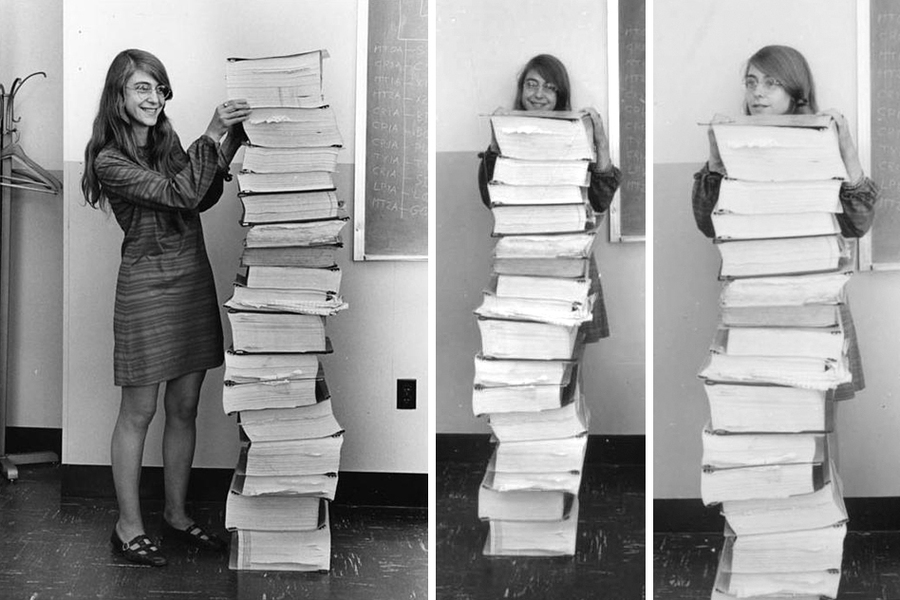
Welcome back everyone. In this video we’re gonna be talking about software engineering. Now you should remember this particular machine the ENIAC, which was the first electronic computer in the United States. Programming the ENIAC was a really slow and laborious process though. To load a program, ENIAC’s programmers Pictured here is Gloria Ruth Gordon, and, well, later Bolotsky, and Esther Gordon would physically rewire the hardware and a new configuration corresponding to the calculations indicated by the programmers. And so you can see them here moving actually the wires from different plug boards for the computer to actually make different calculations and operations work. So the task was made even more difficult by the secrecy involved with the machine. Initially, programmers weren’t even able to see the schematics of the machine and had to pass their wiring instructions belong to the technicians. So the programmers didn’t weren’t even instructed on how the actual machine was built or how it worked. And they couldn’t even actually run their program themselves. So you could imagine that that would be a really difficult task to actually accomplish writing successful programs for a computer that you didn’t even know how it worked.
But this was very similar to Alan Turing’s original conception of the his famous Turing machine. And this machine had carried out hardwired instructions on data encoded as zeros and ones on an infinitely long paper tape. Turing had an epiphany with this machine, realizing that by making this machine read instructions on specific sequences of zeros and ones, as his machine booted, he could encode the program directly on the infinite tape with the data it was actually operating on. Now, this is a huge leap, because before right with this, we had a tyranny of numbers problem where the We’re just getting so complex, that it became nearly impossible to make anything substantial in today’s terms of software.
But now that we can actually store the actual software alongside with the data actually being used the started to simplify the process. These ideas were incorporated into electronic computers by several computer scientists, including J. Presper Eckert and John Mauchly, inventors of the ENIAC computer, as well as John Von Neumann, who was the first to publish such an article about this architecture in this paper, the first draft of a report on The Ed vac. For this reason, a computer architecture allowing for stored programs is referred to as the Von Neumann architecture, and is the basis for modern digital computers. Stored programs also allowed us to develop bootstrap code or libraries of common procedures that can be reused for future programs. And we’re loaded into the computer as it was warmed up. This is an important predecessor to modern programming libraries and operating systems. So as you can imagine a lot of these early computers, you ended up having to actually program basic operations anytime you actually wanted to work with something. So a lot of the software, a lot of things were done by hand, a lot of the things that we take for granted like user input, a lot of the mathematical operations that we use in modern programming languages, all of these libraries that we utilize to make our software a lot easier to write, and which allows them to be extremely functional and easy to read. And these weren’t existing or at least didn’t exist in a lot of the earlier software that was actually being developed. So our ability to store programs along with data and store programs, along with the actual system itself. Made a lot to future programs a lot easier and faster to write.
But the next major invention in software design was the development of programming languages and the associated technologies of compilers and interpreters that allowed programmers to write programs and a higher level programming language that would then later be translated into machine language for a stored program computer. Pictured here is Grace Hopper, the creator of the first higher order programming language flow Matic and influential co creator of COBOL. A very popular or was very popular business programming language. The development of programming languages is especially important in that it allowed us to develop abstractions for simplifying development of software and allowing us to express significantly more complex ideas in computer code without a significant amount of more lines of information and code that had to be made with the software.
But as programming languages diverse From their mathematical roots, and became more expressive, new challenges arose in making sure that programs were clear and easy to understand. This is further complicated by increasingly sophisticated nature of software that sought to accomplish more than earlier programs had ever had. Furthermore, the growing industry demand for software developers had led to often incompletely trained programmers entering the field. And so if you could even code a little bit, you probably could land a programming job. This is a pretty important turning point in the industry here because we had a rapid growth of actual technology. So not too long after world war two ended, electronic computers started to become smaller and more popular and they all of a sudden didn’t take entire rooms to actually build right they weren’t the size of school buses anymore, especially as we approached the personal computer era.
We needed a lot more people to actually program there was a significantly higher demand for software and the demand for that software was even greater yet as far as the functionality would actually go for that particular software. So, as a result of all this sloppy programming, poorly understood designs and really the lack of systematic planning and execution, with these poorly trained programmers led to an era of our field being labeled as the software crisis. This spurred the development of a lot of different new technologies and approaches and approaches for developing software.
Some of the key projects from this period include the IBM O’s 360 project that ran drastically over budget while employing over 1000 programmers, and famously the fair act 25 radiation machines which would regularly display an error to their operators. So as a nurse would come in, and try to to administer a dose of radiation to let’s say, a cancer patient, they would then try redoing the treatment because there was an error on the machine on on the screen or whatever. And they wouldn’t realize that the machine had already delivered a dose of radiation, which led to a lot of patients actually dying or being crippled.
Throughout the software crisis, a lot of important computer scientists made a lot of developments in contributions to software engineering, and one of the more important computer scientists of the day, like Edgar Dykstra and Nicolas Wirth sought to address these challenges through language design and better education for fledging budgeting computer scientists. This 1968 letter to the editor of the ACM journal by Dykstra underscores his concerns with the goto statement, which allowed for a very disjointed style of programming that would make programs difficult to debug and understand as the go to statement would allow you to jump back and forth between steps in your program without any concern for anything else. This and readability of and usability concerns as well as efficiency issues became one of the driving forces behind the evolution of programming languages. Where most currently use programming languages don’t even have a go to statement like Python, and many of the many of the other popular languages that we use today. Other improvements included the addition of modules and information hiding, introduced by David Parnas concepts that eventually involve evolved into what we refer to now as the object oriented programming languages.
In the same year, Margaret Hamilton, one of the NASA engineers responsible for simulating the Apollo missions on a computer. One of the most involved computer simulations attempted to that time, coined the term software engineering to describe the role she had played The stack of documents Next to her is actually one of the simulation results from that effort, which helps underscore just how large software projects were growing at that time.
Now that we’ve talked a bit a little bit about the history of software development and software engineering and how it’s evolved over the years, what are some of the key activities that we actually engage with in this process. Now, you’ve already used and worked with a lot of these already, even if you haven’t really made the connection to them yet. Software Engineering overall will come with quite a few different processes along with it. But overall, you can kind of expect these six different stages.
Now, to begin the process off, we’re going to start with requirements gathering are going to actually go around and collect information about the software that we’re actually being tasked with to develop. So this involves with going and meeting with clients meeting with users meeting with business folks meeting with just about Anybody and everybody that might be a stakeholder or involved with actually using that software or funding that particular kind of project.
Now, once we have gathered all of the requirements for the software, then we can make the jump into the software design. So here we’re going to start to architect the project and lay it out overall, but we haven’t actually even done any programming yet. That doesn’t actually typically happen until the design has been actually completed. So once we actually start the implementation, then after the code has been finished, or at least a stage of the code has been finished, that code is then split off into the testing phase. Sometimes the implementation and testing phase, you might see done as one as if you’re on a small team or depending on the kind of approach you’re actually taking to the development lifecycle.
But after the software has been fully tested, then it gets deployed or installed. And then it goes into like a maintenance mode, right. So a lot of times you get the first Windows updates and various other software updates on mobile apps and games and everything in between. So that’s the maintenance phase, right, where we’re trying to update patch, fix anything that may actually been broken, or things that we didn’t catch during the testing phase. But you see that now I’m back at the requirements gathering.
Most of the software development life cycles that we actually see an encounter are a never ending cycle. Software is never perfect the first time around that we actually build it. So more often than not after creating what we refer to as a prototype. We’re going to end up going back to the requirements gathering stage, talk to our customers, talk to our consumers, talk to our stakeholders, and give another shot at it. Whether or not whether it’s just a, a simple update, or feature addition, or even a complete rewrite in some cases if we didn’t get it right the first time. But let’s take a look at some of the early software development life cycles that were developed. Now, you’ll notice that these each of the activities that we just talked about before lend themselves very well to a systematic step by step approach, where each activity is followed by the next and we kind of loop back onto this.
This is essentially the approach that was developed as a standard strategy for software engineering after the work by Margaret Hamilton in the early 1960s. And over the next few decades, an approach that we call the waterfall model of software development for reasons obvious from the graphic, where each phase flows from the next into a highly linear fashion now In the waterfall development, as I mentioned, right, this is a very linear process. This isn’t like the software development lifecycle that we’ve showcased earlier, where we start with the requirements gathering. And we cycle through each phase. And we end back up at the beginning of the waterfall method assumes that each phase is done in one shot, so there’s no reduce.
So we gather the requirements and design the software, implement it, test it, so verification, and then we go into the maintenance mode. So of course, we install and deploy the software in between there. But once we’ve deployed the software and enter maintenance mode, we’re not going to actually be going back and doing more requirements gathering or redesigning anything, it’s just some simple bug fixes at that point. So, it emphasizes the waterfall model emphasizes that the actions are arranged as discrete phases in sequential order, although depending on the model that you actually look at some splashback is acceptable. So if you imagine an actual waterfall, some water gets splashed back up and falls back down. So maybe we get to the implementation phase, but we recognize that our design is severely flawed. So we may bump back up, change the design a little bit, and go back down into the actual coding phase.
But here, the entire system, and the waterfall model is implemented, designed and deployed all at once. So planning, scheduling, target dates, budgets, all of those things are set in advance. Most of the time, these are often set by contracts. So there’s really no flexibility there with as far as funding and deployment dates go. A lot of times with the waterfall model, there’s a lot of extensive documentation and very tight control. So this is a very heavily managed process. So this is really useful for processes that require a little A lot of structure. And we’ll talk about some other models here in a little bit that have a lot less structure, and that offer a much more flexible approach to software design.
Additionally, during this time, scientific management techniques were adapted for use in the management of software developments. One of the landmark books capturing this evolution was Barry Boehm’s Software Engineering Economics book, where he argued for considering trade offs between adapting existing software and creating new software on economic terms. And so we use statistical analyses to develop equations like this one, seeking to equate development time in main years to the metric of software lines of code, or SLOC. Now, there are there’s a lot of debate around measuring the productivity of let’s say, developers and cost of software based off of the number of lines of code that are actually produced. And there’s a lot of fallacies behind that metric as well. But a lot some people actually some fall into that trap.
Another book from that particular time period refutes some of those both some of those arguments as I mentioned, they were very controversial. But this book, the mythical man month, details many software engineering management fallacies. Like, for example, adding more programmers to a late project will absolutely right help it finish sooner, but not so much. In practice, bringing new developers up to speed consumes much of the current team’s time, and overall slows the development. So let’s say you’ve been working on this really big important project for nine months. But you are a couple, maybe a month or two behind schedule. So management comes in brings in new developers to try to help get you back on track. But it actually ends up putting you back farther in your time schedule because you had to stop your productivity to get the new people caught back up to speed.
Another fallacy here that is discussed in the mythical man month is the use of crunch time. Crunch Time is typically portrayed as an increase in productivity, right. So, you know, spending, you know, 60 to 80 hours a week to meet that deadline. So, pulling 18-20 hour days, programming all night, I’m sure you have probably done this when studying for a really big exam. Crunch Time doesn’t necessarily increase productivity. Studies have actually shown that a breakeven point for let’s say software development lies around about 35 hours. There’s been research that shows about 30 a year your average limit for a software developer is about 30. 35 hours of programming per week. Beyond that, a fatigue programmers introduce more bugs into their code at a faster rate than they’re actually removed. So that ends up costing a lot more money and time because they’re, you know, fatigued. Developers that have just been coding for too long or going to be more prone to produce bad code. I’m sure some of you some some of us have experienced this as a student, as I mentioned, as you’re studying, you know, when you’re really exhausted, or have had way too much caffeine are way too much coffee. You may not be studying as efficiently or or productive. Your productivity may not increase proportionally to the amount of time that you’re you’re actually spending versus the amount of time you’re spending when you weren’t exhausted.
Let’s take a look into a few other different methodologies in software development. So this one is in complete contrast to the waterfall model of software development and pretty much all other development methodologies. Because this methodology, there really isn’t anything to it. It’s generally known as cowboy coding or code and fix. Now, this in many ways, is the anti software engineering approach, where planning, testing documentation at pretty much everything, all of that is ignored, or immediately writing code. And predictably, this leads to a lot of what we refer to as spaghetti code. And so it’s just mangled structure that has really no clear way to it at sprinkled with sub optimal algorithms memory leaks, structural issues is just a mess, right? Imagine getting out a box of Christmas lights that were just thrown into a box and in January, and you go back in December, try to put those Christmas lights up. And magically, they’ve aimed together into this big ball that takes hours upon hours to actually unravel. And sometimes it’s just easier to throw it away and start from scratch.
Even more unfortunately, with this methodology of cowboy coding, this is actually unfortunately very much how most students learn to approach software development and their early assignments. And it’s often carried with them into industry. So the sooner that we can actually start to teach design structure and this process, the better habits that you will develop, especially as you start getting closer to working to working to an internship and into To a full time job.
But not surprisingly, issues in software engineering are typically coupled with periods of surging growth for a field of computer science. And so this graph here based off of data collected by a tabulate survey tracks the growth of Bachelor’s of Computer Science degrees since 1966, up through about 2010. Now, you’ll notice the two very clear spikes in this graph, one peaking around 1985 and the second around 2004. That first rise was a big issue here for K state and many other universities that that matter, to and to meet the growing demand of students with the limited faculty available to graduate students taught and many of the undergraduate courses, similar measures were employed at other institutions likely compromising the quality of preparation for an entire generation of software engineers because people were thrown into teaching positions that really weren’t that well qualified to teach those particular topics are experienced enough.
A similar trend occurred during the second peak, although thankfully not so much with us. But hopefully you can maybe guess what the driving force was behind that growth rates at that time, right. So this peaked around 2004. That was around the.com. Boom. So the first search that we saw began in the early 1980s when the personal computer started to be introduced. And so that spikes the first surge and the demand for computer science degrees, and then the second peak reflects the dot com bubble. So as the internet came out in 1990, we saw a huge burst in the late 90s of companies thinking, Ah, well, we can make it big if we get on the internet. Okay, and so we saw a huge surge In the need for computer science. But after the.com bubble burst, which burst in the early 2000s, we saw a rapid decline in the demand for computer science degrees. But thankfully, over the past few years, we’ve since then we have seen a increase, and the demand for computer science or an increase in the number of degrees awarded in computer science. And we haven’t seen that die off quite yet.
But with the growth of the internet, Internet companies and the eventual collapse and the success of all the survivors to underscore the need for a more reactive and flexible style of software development that was possible with the waterfall model. So the dot com boom, sparked a lot of different kinds of needs of technology and software, especially with the invention of the internet, of which we had never actually developed software for something like that before. So the web needed to be what robust, secure and most importantly, scalable. And so that meant cowboy coding couldn’t meet that need either, even though it was super flexible, because we could just start with no planning whatsoever. But that often led to very insecure software and software that really didn’t scale well. So new strategies as a result of the dot com boom, emerged to create more robust software engineering approaches, and these were started to be employed more widely.
One of these of course, was just simply prototyping which is especially useful for developing experimental or difficult to estimate systems. And so the idea here right is to build a prototype, establish the base functionality, complexity and worth wildness of the of the specific product right. So this begins with implementation or coding and then leads to other activities, like requirements gathering and software design. So try something out and see if it works. See If the Customer likes it. If they liked Or let’s say they like this, but not that let’s keep things that they like and throw away the stuff they don’t want. So this is pretty much the cowboy coding or the code and fixed process with a more developed and structured approach, right. It’s not just a standalone process. There’s a lot more involved and there’s a lot more structure here.
The iterative development process, or the iterative development model breaks down software development into much smaller segments. This allows for a lot more change and variation to the development cycle. So the iterative development process works by working through many waterfalls. And so if you look at each one of these chunks here, each one of these stages, they’re pretty much the waterfall process. And so overall requirements are gathered, then we analyze those requirements develop, implement test, and this is a cycle right? In this case, our waterfall is circular so we can keep on trying Go Go, go, go go. And then we’re going to release a prototype or a version of our product. As we go through this each time a release, we demonstrate that to our customer. And get feedback and then we’ll work that back into our next cycle. And so we just keep on iterating this until we are doing our final release to our customer.
One more different developments that we want to talk about this time is actually proposed by Boehm, this combines prototyping and the waterfall development is very similar idea to iterative design. The spiral development model focuses on risk assessment and management by breaking projects into smaller parts, allowing for the evaluation and change as each part is individually finished. And so this works off of four main segments. So you are going to determine the objectives, alternatives and constraints of that particular iteration. So that small part, evaluate alternatives, identify and resolve those risks. So we want to try to match negates the risks because those risks, right, the more risk, the more cost is actually involved with the project. And then you’re going to develop and plan for the next iteration. So as you start to cycle out here, right, so you’re starting small, the center here, you’re going to start with very small projects, right. And as you complete those smaller projects, the base of the foundation of your software that’s going to slowly grow out, and you’re slowly going to introduce more things that are needed in the project, like different models, different prototypes, more testing, and the closer you get to the outside edge of the spiral, the closer you’re going to get to deployment. But this is again, right like iterative design, much more flexible, and overall, much more appropriate to what modern software actually lends itself to.
But even more so after this We actually come into something that’s very popular industry today called the Agile process. These methodologies that we’ve talked about so far were to being developed by software engineers and high level planning positions. A new philosophy was emerging from the rank and file developers which, as expressed in this Agile Manifesto, the manifesto reads as we are uncovering better ways of developing software, by doing it and helping others to do it. Through this work, we have come to value individuals and interactions over processes and tools, working software over comprehensive documentation, customer collaboration over contract negotiation, and responding to change over following a plan. That is, while there is value in the items on the right, we value the items on the left more. So while agile is often thought of as, as a software engineering process By itself, it’s not. Rather it’s a guiding philosophy that can be applied in conjunction with many other software development approaches. That said, it clearly works better with something like iterative or spiral development or any other reactive styles of software engineering than the more rigid approaches that embodied the waterfall approach. And so as part of the reading, I’m going to actually ask that you go check out the Agile manifesto.org website and honor they have all the principles that are assessed with agile development and kind of embody what agile actually means.
But overall in the Agile process, you’ll typically see something like this agile as it stands right is the philosophy behind it as extreme flexibility. In this sense, you work off of mostly what we refer to as sprints. So these small Sprint’s will always have some sort of deliverable. product to the consumer or the customer. So it’s looks very similar to what we see with the software development lifecycle and a lot of the iterative or spiral processes where you brainstorm or gather requirements, you design prototype, develop, you QA. So you test and test and test and test. And then you deploy. And as you deploy, you do a little bit more testing, and you deliver that product to your customer. Or maybe you deliver that to the next person up in your organization. And all that feedback is then worked back into the next iteration into your next sprint. And so typically, what you’ll see with Agile process of the Agile process or Agile software development is that each sprint will focus on one or two small features of the software. And once that feature is actually completed, then the that particular developer will move on To the next sprint with the next development of either that same feature with modifications that were given to them by the consumer, or moving on to after completing that feature moving on to the next.
Another improvement that came in the mid 90s was the development of a suite of standardized diagrams for modeling software. The Unified Modeling Language, or UML. UML allowed for complex software systems to be diagram discussed and shared between developers and an easier to interpret form. Because before then there was no standard for documentation or not necessarily, but there was a lot of complex software being developed and each programmer would document and diagram in their own unique way. Just like what we would have, we have our own unique way of speaking and writing. Each developer had their own way. of not only just writing their own code, but also diagramming and and discussing about that code. And so UML offer a standardized way to actually share the overall structure interactions. Things like the activity or sequence or flow of the program among different developers, actually was someone who’s actually been trained with you to interpret and read UML could understand the software at a much higher level, a much deeper level, even without knowing how to actually program. But for now, this is going to conclude our discussion on software engineering, software development. There’s obviously a lot more here that we did not cover. In future classes we’ll take a much deeper dive into the architecture, modeling and development of software.
Read Pattern on the Stone, Chapter 8.

In this module, we’ll discuss the field of human computer interaction or HCI, sometimes referred to as computer human interaction, or CHI. It is the study of how computers and humans interact and how we design computers to better support humans in that efforts. HCI is one of the fields that we’re going to look at it throughout the semester, we’ll do this several times.
The field of HCI has a few goals that are very important for us to keep in mind. First and foremost, HCI aims to try and make the world a better place through the use of easily accessible technology. It allows us to work to understand data that is being presented to us, and it helps people interact and communicate with one another using modern technology. But Finally, and most importantly, the major goal of HCI is to give people better control over the tools, computers or machines that we’re using in our daily lives.
So how do we do this? Important part of the field of HCI is studying and designing and applying all the things we learn about interactions between people in computers. Sometimes we study how people interact with computers. And sometimes we have to study how people interact with other people, and how we can bring those ideas to the computer. And so to do this, we end up using results from a lot of different fields, not just computer science, but the fields of cognitive and behavioral psychology, design, Media Studies, graphics, art, music, all of these things can go into the field of human computer interaction.
One of the pioneers of the field of HCI is Douglas Engelbart. In 1950, Douglas Engelbart had graduated college, but really had no idea what he wanted to do with his life. And so he set out to try and determine how he could have a greater impact in the world and came up with this really interesting idea that we’ll look at in just a second. But his ideas really lead to the field of human computer interaction as we know it today. And he’s responsible for it. Large part of how we use computers, I think you’ll find it really interesting to see the things that he came up with during his time. So as we talked about Douglas Engelbart was a student in the 1950s, and was really struggling to figure out what he wanted to do with his life. And so eventually he came up with this idea for a motivation to help him work in computer interaction. So first and foremost, Douglas Engelbart decided that he wanted to make the world a better place. That’s all well and good, but you really have to understand how to make that happen. And he realized that to make the world a better place, it required a large amount of organized effort. It wasn’t anything that one person could do on their own. So how do we get that organized effort, but we have to bring together the collective intellect of all the people in the world working to solve these really big problems. That is really the key. And so Douglas Engelbart realized if that process was somehow made easier, he could effectively boost the work of every person working on all of these large Scale world problems. And that is what led Douglas Engelbart to the field of computer science and HCI. He realized that if he could make modern computers more effective, more efficient and easier to use, that that would, in effect, boost the effort or everyone working on these problems, because it would allow them to come together and harness their collective intellect to put forth organized effort to make the world a better place. So as we said, computers are really the key here and that’s what Douglas Engelbart realized.
One of the greatest creations of Douglas Engelbart work is the computer mouse shown here. It’s the first example of a interaction device built specifically for a computer that really revolutionized how we interact with computers. He developed the computer mouse in 1967, while he was working on the design of a computer system called the online system or in Is that we’ll look at in just a second. And he originally patented it as an X Y position indicator for a display system in a video that will take Look at he actually jokes a bit about why it’s actually called a mouse today.
But as we said the mouse is just a small part of what Douglas Engelbart was working on. His true work revolved around the online system or in NLS computer system that he developed. The NLS was really the world’s first modern operating system to include features such as a mouse hypertext links that you could click on a raster scan video monitor that actually gave live feedback to the user, the ability to do screen windowing, where you could have multiple things on the screen at the same time, he was able to use that system to build presentation programs that are very similar to what we do with PowerPoint today. It allowed him to organize information in radically new ways that had never been seen before on a computer system. And it even allowed for collaborative editing and messaging, very similar to the tools that we use today on the internet.
And the amazing thing about this system was it was demonstrated in 1968 in what has been called the mother of all demos. Douglas Engelbart demonstrated all of the features of the online system during a single live demonstration in December of 1968. He assembled over 1000 computer professionals in an auditorium. And with double Douglas Engelbart sitting at the front at a computer console. He seamlessly demonstrated the power of his NLS system, showing new idea after new idea to these people. And he left his audience completely spellbound. And to this day, it still stands as one of the most important and most unique computer demos of all time. Oh, and by the way, he was actually using it to control a computer that was over 30 miles away. So it was done remotely. And to put this in context, remember that December 1968, is several months before we landed on the moon in July of 1969. So even though we were sending people to the moon, we’re in spacecraft that had less power than a graphing calculator. Douglas Engelbart was setting the stage for a computer lead to revolution in how people use computers today.
The best part about the mother of all demos is that a recording of it exists so that we can watch the whole thing even today. As we mentioned, he combined some real cool state of the art technology in this single demo. He used live video projection, he used teleconferencing and video conferencing. And for a lot of people in the audience, it was the first time they had even seen a live computer display something that we take for granted today. So on the next page, we’re going to take a look at a few short clips out of this mother of all demos, and we’ll have some short discussions about what exactly he’s showing on these clips.
The full video of the Mother of All Demos is linked below, but it is nearly 2 hours long. While we’d love to have you watch the whole thing (and you are more than welcome to do so), we wanted to highlight a few of the more important parts. Listed below are the timestamps for a few important sections and a bit of discussion about each one. Feel free to skip around to watch a few of these sections to better understand what Douglas Engelbart was presenting.
On the previous page in NLS was a very revolutionary system. Unfortunately, it was very hard for the average user to use. And so it really never could gain that mainstream reputation that it wanted. So we had to come up with an easier way to use modern computer systems.
And as the story goes, and engineer one day was staring at the top of his desk thinking about how to solve this problem, and that solution came to be known as the desktop metaphor. What if we build a computer system that looks and acts and feels like the things that we’re used to in the real world, we can have a desktop with different things open on it as we’re working. We can have files and folders full of files that allow us to organize information, and we can move things around quickly and easily to get us different views of the same thing.
This is what most modern computer systems were built around, and it was first introduced all the way back in 1970. This picture shown here is from the Xerox star workstation in 1981, which was one of the first real mainstream computers to use the desktop metaphor. Of course, in those days, one of the things that computer companies were really well known for is borrowing or stealing other ideas from other companies. And so Apple stole basically the same desktop metaphor idea for its Macintosh desktop from 1984.
And there’s always been a little bit of discussion about who actually came up with it first, this was actually dramatized in a TV series called The Pirates of Silicon Valley. So let’s take a look at a short clip from that TV show to give you an idea of what things were kind of like at that time.
So now that we’ve seen some examples of historical computer interactions, let’s talk about what it might take to make a good computer interface today. Think about the computer systems that you interact with on a daily basis. What about them makes them easy to use or difficult to use? Would your answer change if you gave that computer system to a toddler, or maybe your grandmother or an elderly person? So really good human computer interaction or good computer interfaces can depend widely based on the needs of the audience. Of course, there are some things that we can think about that make good human computer interactions. For example, we want it to be functional, it needs to do what it says it does. It needs to be reliable, it should always work the way we expect it to. It needs to have a high level of usability. So it’s something we can easily and effectively work with. It should be efficient. We don’t want to have to click 18 times to open up a single web page do we? It also should be maintainable both from the ideas of the user, it should be easy for them to keep their computer up and running. But it should also be maintainable on the software side for the developers that are building these apps. And one of the things that I think is often overlooked in the field of HCI, is it should be portable. We really want the same ideas to work across multiple different devices and even multiple different paradigms. And that’s something we’ll talk about a little bit later.
To really develop good HCI we have to follow this iterative design process where we start with an existing device, we analyze that device, we check our requirements, and then we can slowly make things better. It’s really interesting to think how computer systems have developed over time. And there’s some great YouTube videos looking at this, for example, considered the original iPhone design versus what we have in our modern iOS, or consider some of the earlier versions of Windows compared to the modern versions we use today. While those systems are very similar, we can see that there’s been a slow iterative design process that has slowly improved the design over time, based on the changing hardware and our changing understanding of good HCI.
Of course, good HCI also relates to a lot of different fields. We have to think about things like psychology, such as the fields of memory and perception. How do we remember things? How do we perceive things on our computer? We have to talk about sociology and how interacting with computer changes how we interact with other humans. We look at things like cognitive science, we look at ergonomics, how easy it is for us to use a computer system, we can think of things such as graphic design and interaction design, what colors and shapes and buttons would tell us. We can even think of things like speech language pathology, should our computer refer to itself in the first person or the third person? How should it interact with us? And we can even think of really interesting fields such as phenomenology, the study of consciousness, how do we make things on our computer such as that we are consciously aware of What our computer is trying to tell us. And we’re not just ignoring it and clicking next all the time.
So one interesting case study from the field of human computer interaction is the case study of automated adaptive instruction. Automated adaptive instruction is the idea of providing the user with instructions based on what the user has done previously, and what we think are some possible next actions of the user. We’re all familiar with our phones autocorrect system, how it can predict the next words we’re trying to enter. Gmail recently has done this as well. That’s kind of the same idea. But instead of just filling in words, it’s actually telling us how to use the computer system and how to do what we want to do next. This really came about in the 1990s as users were getting used to the personal computer, but they were becoming overwhelmed by the complexity of the technology. And companies such as Microsoft turn this into a very lucrative area of research.
And so probably the most interesting case study from adaptive instruction is the computer program known as Microsoft Bob, hopefully you’ve heard of Bob, but if not, this will be a really interesting thing to talk about. And I get really excited talking about this because when I was young, the first computer my parents bought came with Bob pre installed. And so my first computer interaction was actually with Microsoft Bob. This is what Microsoft Bob looks like. The whole idea behind Microsoft Bob was to take the desktop metaphor to the next level. And instead of having a desktop for our computer, we could mirror an entire house. And so our house would have a whole lot of different rooms, we could have the living room, where in this room we have things such as a Rolodex that represent our address book, we have a money bag that represents our finances. There’s a checkbook sitting on the table that represents our Quicken or our check our money software. And that was really the idea you would have things in your house in Microsoft Bob, that mirrors the things that you would use in the real world. And by clicking on those objects, you would opened the programs that related to that. And then of course, you could have different rooms, you could have a living room with all of this, you could have an office with different things, you could have a kid’s room with all the games in it. And so it was a really neat idea.
But of course, the automated adaptive instruction part is the little dog that we see here. This dog is called rover, and rover was there to try and help you navigate Microsoft Bob, it would offer to do things like help you find a program, go to another room, add something changed something, anything you wanted to do, you could interact with rover and rover would help you figure out how to do it. And it was this really neat idea. Unfortunately, I think Microsoft Bob really wasn’t quite ready for primetime. And graphically, it doesn’t look very good. And in fact, most computer users had gotten used to the desktop metaphor. And so the power users weren’t exactly excited about it either. And of course the biggest nail in the coffin was Bob itself wasn’t that great of a piece of software in some ways. It was kind of buggy and did crash a lot. How There are some people that really are big fans of Microsoft Bob even today. And so if you look online, there’s some great videos of people who have installed Bob even on a modern computer just to see how it works.
Of course, this did lead to some ideas that stuck around. For example, rover became the search assistant from Windows XP. And of course, this is the source of the infamous Clippy office assistant from Microsoft Office 97. Again, it was the same idea. Microsoft Office has a lot of features that most users don’t know how to do, such as mail merge. And Clippy, even though Clippy might have been a little bit annoying, was perfectly capable of helping you figure out how to do that. And so it kind of got a bad name, but it did have some neat ideas.
The big lesson learned from these assistive agents is companies were trying to teach users how to use computers, instead of trying to design computer systems that work the way users expect them to. And so in a lot of modern computer design, instead Have all of this instructive bits, you see us trying to more and more build computer systems that act like we expect them to. A great example of that is on your phone. If you scroll up at the top of a web page, it tries to refresh the webpage. This is especially notable on social media sites like Twitter or Facebook, you’re scrolling up looking for new content. And so it immediately reacts to that and does what it expects you to think it wants to do.
So of course, there are a lot of virtual assistants out there today we have Clippy. In 2011, we had the release of Siri on Apple devices. We’ve had Google and Cortana. And now we have other devices such as Alexa. And so we’re really into the smart, the age of the smart assistant where almost every home has a smart assistant in it. Almost every device has the capability of using one. And so we’re really seeing this come into its prime today. So what were the big lessons learned? Well, of course, this led to a lot of different ideas, such as searches on Google, if you’ve ever searched for something on Google, and you get that Searching? Are you sure you didn’t mean X? That’s an example of adaptive instruction. It’s telling you how to do things on Google.
We also see context clues on our touch interfaces, where if we swipe left and right, when there’s nothing there, it will still let you swipe and show you that there’s nothing over there to be able to swipe to. And so like we talked about earlier, the big legacy here is, instead of trying to change human behavior, we want to try and change the program to fit the expected behavior of the human. Or to put it more concisely put things where people expect them to be.
One person who’s very active in the field of HCI today is Don Norman. Don Norman was a 2006 Franklin medalist. And he’s really famous for writing a book called The Design of Everyday Things, which if you haven’t taken a look at it, I encourage you to at least look at the front cover of that book and see what he’s talking about. Don Norman is a real big proponent of designing things to be how they’re expected to be used instead of design just to be interesting. And he talks about some really great examples of designing for everyday things. And so after this video, we’ll take a look at a short clip of Don Norman talking about some of his work, and hopefully, you’ll start to see the things that he saw in the real world that helped us understand modern design.
So one of the important things to remember in HCI is that iterative design process and designs change over time. For example, on this slide, the top picture is a picture of Microsoft Word from version two 2003. And the bottom picture is from a much more modern version of word that we use today. In 2003, the version at the top was very well regarded, it had a toolbar with lots of easy to follow buttons. And a lot of people got used to it and really liked it. And so in 2007, when they switched from the toolbar design to the ribbon design that we use today, there were a lot of users that really didn’t like that design. And if you get down to it, it really turns out that those users didn’t like the design, not because it wasn’t a better design. They didn’t like it because it was different. And so one of the things we’ve struggled with in the field of computer science is design changes for change sake is not good, because a lot of users don’t like change. But if we change things for the better, eventually users will get used to it. And thankfully, we’ve seen over time that users have very much gotten used to the new ribbon style and they do understand that it is much more efficient and much easier to use than the old toolbar style, but there’s always still little bit of fear of change that always comes into this.
Another good example of this is Windows, we’ve gone from Windows XP to Windows 7 to Windows 8 to Windows 10. And each time we’ve changed a little bits of how the Windows computer system works from different toolbar designs, two different Start Menu designs, two different designs for things such as the control panel and touch interfaces. And each one of those designs might be based on a lot of really good research, but it’s changed and a lot of users are very resistant to change at first. But of course, some changes are really good. For example, in Windows XP, if you had a blue screen, you would get something that looks like this. This error message isn’t really all that helpful is it? It’s got a lot of technical details. But for most normal users, it just scares them and they don’t really know what to understand. And so a more modern computer system has a little bit friendlier, have an error message that tells you what’s happening and it tells you what’s going on but it doesn’t just bombard you with more data than you actually need.
So what is the future of HCI look like? It’s really hard to tell, but there are tons of things going on. After this video, we’ll post several videos for different views of HCI. And some of the things that have been out there in research or in industry today, for example, different user interface concepts such as 10 GUI, different ideas around ubiquitous computing, such as the Google Glass project from a few years ago. We can look at 3d tools today, such as the Oculus Rift, and some of the new 3d virtual reality tools. And we can even talk about accessibility and how we can design computer systems that use just a single finger to allow you to type text very, very fast with a minimal amount of inputs. And so I hope by looking at some of these videos, you’ll be inspired by the different ways that computer systems can be interacted with beyond just the keyboard and mouse that we’re used to today, and it will encourage you to think about different ways that we can build computer systems in the future.
Read Pattern on the Stone, Chapter 9.