Intro CS Textbook
This is the textbook for Intro to CS.
This is the textbook for Intro to CS.
The basic building blocks of computer science theory and programming, along with a bit of history!
In this module, we will dissect what computing science really is. To do this we will step back in time to determine what the motivation was for computing machines, the products of those needs, and how they served as inspiration for modern computing.
In this course, we’re going to ask ourselves, what is computing science? It’s a really important topic that we’d like to cover throughout this course. But it’s also one that’s very difficult to understand. So when we try and understand the topics such as what is computing science, we can ask ourselves the questions: who? what? when? where? why? and how? And while I do this, I realized the question of “how” is really the best way to approach computing science. Specifically, I like to think of computing science as the study of how - how we can make things faster, better, more efficient, more accurate and more secure using computers. But that becomes a really interesting statement because we haven’t discussed exactly what a computer is.
So before we can look at all this “how”, let’s ask ourselves: “what is a computer?” We’re all probably familiar with the modern computers that you and I have in our homes and around us today, but is that really the best definition of what a computer is? Or is there more to it? That’s what we’re going to take a look at in this video. So to really understand what a computer is, we have to go back a little bit and look at some of the earliest examples of devices that might be considered a computer. And it turns out those devices are really wrapped up in the history of mathematics.
So on this slide, we see some mathematical equations, such as the equation for the exponential function, which is this long, repeated division. We can have sine and cosine and all of the trigonometric functions. We can have limits which are the basis of calculus, and we can even have logarithms which show up a lot in statistics and finance. And all of these functions are very, very difficult for people to calculate by hand. So how do we find the values of, for example, sine of 46 degrees? Using modern technology, we can find these values using some very interesting tools such as computers or calculators, but in the 1600s, they might have to use something such as this.
This is a book of math tables from 1619, and it gives the value of sine, tangent, secant for all sorts of different angle values. And so a table such as this might be used by engineers, mathematicians and scientists whenever they need to find these values for their work. And in fact, if you’ve taken a calculus class, or trigonometry class or geometry class, your textbooks probably had tables like this in the back of the book. And as recently as the 1960s and 1970s, engineers would have had little books full of these tables that they carried with them all the time before the rise of the modern pocket calculator. But of course, this begs the question of how do we get these numbers in these books? We don’t have computers, we don’t have calculators.
So how did we do it? And it turns out that that lies in the work of a lot of early mathematicians such as John Napier, who helped describe the logarithmic function, and Jacob Bernoulli, who helped describe the exponential function. And so one way that you could populate a book full these values is work with the best mathematicians at the time and have them perform all of that mathematical work. And this is important because in the 1600s, not many people had the level of mathematical training required to work with those really complex functions that we saw earlier. But of course, this is not a really great use of their time. So we tried to find ways where we could do better and easier mathematics to find those complex values.
One of those big improvements was the creation of Taylor series. If you ever take a calculus class, you’ll learn all about Taylor series. But the big thing to understand is a Taylor series is simply an infinite polynomial that expresses values of those complex functions. For example, the exponential function can be expressed as the infinite polynomial, one plus x plus x squared over two factorial plus x cubed over three factorial. And so we’ve reduced this value down to a set of individual terms. And so if we can calculate the value of each individual term and add them together, we can find the values for the exponential function. Of course, this is a little bit easier than that earlier statement, but it’s still very, very complex mathematics that would take a lot of work.
Enter the work of Sir Isaac Newton, Isaac Newton, you’ve probably heard of lots of times in your math and science courses, and he was very impactful in a bunch of different fields. But for this particular field, we’re looking at one specific thing he created that’s not very well known, which is the method of divided differences. And so Newton’s method of divided differences allows you to find successive values of a polynomial, any sort of polynomial that you can create, including these infinite polynomials for Taylor series. You simply cut them off at a particular value, and then you use that polynomial and Newton’s method of divided differences to find those values that you would place in a book. So let’s look at an example of Newton’s method of divided differences to see how it works.
To understand Newton’s method of divided differences, we have this example with a polynomial: two x squared minus four x plus three. Then we’ve created a table below, where we have the first column that gives values of x and the second column that gives values of the polynomial applied to that value of x. So for example, if we put x equals zero into the polynomial, we’ll get the value three. If we put x equals one in the polynomial, we’ll get two minus four plus three, which is one, and so on. So we can populate the first few values in this polynomial column very easily using simple mathematics.
Once we’ve got a few of those values, then we can build this first differences column. And so the differences column will take the value of the polynomial at one minus the value of the polynomial at zero, and so we’ll have one minus three, which will give us negative two. Likewise, for the next value, we’ll take three minus one, and we’ll get the value two. And so we can do that to fill out the first few values in this difference column.
And then we’ll do it again to make a second difference column. So here we have two minus negative two, which is four. And what Newton realized is if you do this enough times, you’ll eventually reach a column where all the values will be the same. And you have to do that for each order of the polynomial. So this is a polynomial of order two. So that means we need two division, or two difference columns to get to this column, where all the values will be the same. So now, once we know that this column is four, we can put in four for each of these values.
And then we can use those to work forwards through the table to find other values of the polynomial. So now to fill out this value right here, we can do four plus two, and we’ll get six. Then we can do four plus six to get 10 here, then we’ll do four plus 10 to get 14, then we can work forward again and fill out the polynomial column where we have six plus three is nine. 10 plus nine is 19, and 14 plus 19 is 33. There we go. That’s how you do Newton’s method of divided differences.
This slide shows a completed table that is a little bit easier to read. And we can see that we got the correct values. Now this method of divided differences does have one major issue, and that is it’s very susceptible to human error. For example, what if we add four plus six and instead of getting 10, we get 11. Then what happens? Well, if we do four plus 11, here, we’ll get 15 instead of 14. Then if we do six plus three, we get 9, 11 plus nine, now we will get 20 here. And then likewise, if we do 20 plus 15, instead of 33. We will get 35. And so as you can see, by making one small error right here, we’ve actually made all of the subsequent values in the table invalid. And that’s the real problem with Newton’s method of divided differences. As soon as you make one error, it invalidates everything after it. So while it’s a very powerful tool, it still has a big weakness.
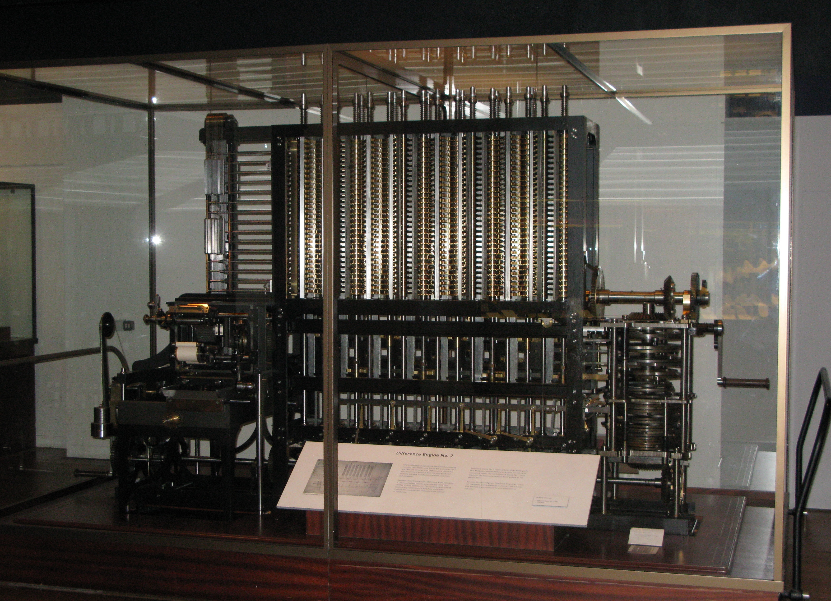
And the real idea is how can we solve this weakness. And that was of interest to Charles Babbage. Charles Babbage was an inventor and a mathematician in England in the 1800s. And he was really interested in creating ways that we could perform these repeated calculations without the risk of human error. And he decided that it was possible to build a mechanical device that could perform these mathematical operations completely, repetitively without any error. And during his lifetime, he actually built a small prototype of this device that he called The Difference Engine, and he built blueprints for a much larger scale version of it, but that version was never actually completed during his lifetime. A few years ago, those blueprints were in the possession of a Computer History Museum and they decided to try and build a device based on his blueprints and see if it would actually work. And surprisingly enough, it totally worked. So let’s take a look at a video of that completed Difference Engine that was built by a Computer History Museum and see how it works.
The director of the Computer Science Museum’s Babbage Project demonstrates how Charles Babbage’s Difference Engine #2 works. While Babbage himself was not able to build the machine in his lifetime, a modern builder created it according to Babbage’s instructions. Through this creation, computer scientists have been able to prove that the Difference Engine works exactly as Babbage intended!
WIRED. (2008, May 2). Babbage’s Difference Engine No. 2 [Video]. YouTube. https://www.youtube.com/watch?v=0anIyVGeWOI
Charles Babbage designed many different engines during his lifetime, but very few of them were actually built.
In the previous video, you saw a completed version of the Difference Engine built very recently, which we actually see here. And his Difference Engine was very revolutionary because it proved that you could build a device that was purely mechanical, that could perform calculations. But the difference engine was actually a very small part of Babbage’s overall vision for building these mechanical computational devices.
He also designed another engine that he called the Analytical Engine, and it was never completed during his lifetime and thus far it has not been completed in modern day time either, but there are small parts of it that exists. For example, this is one small part of it that is in a museum. The analytical engine would have been a true multi-purpose computer. Instead of just performing Newton’s method of divided differences, it was capable of performing all sorts of different mathematical operations.
Babbage’s Analytical Engine would have been programmed using input cards, such as what you see here. And one surviving portion of the Analytical Engine is the Mill, which is a general purpose computational device that can perform all sorts of different mathematical operations. It’s very similar to the CPU in modern computers.
In addition, he would have created a device called the store, which was capable of storing and retrieving up to 1000 numbers at 40 decimal places, which is roughly 16 kilobytes of data, which is really respective for the 1800s. And parts of the design for the store were actually used in the design of the Difference Engine, which is the picture you see here. So what have looked very similar.
And so because of all of his work, designing and thinking about how you would build these multipurpose computational devices, we refer to Charles Babbage as the father of modern computing. Unfortunately, a lot of his designs were forgotten over time. And it wasn’t until very recently that his work was really recognized as being so revolutionary in the history of computing science. In a later lecture in this class we will actually analyze some more work of Charles Babbage, specifically the Analytical Engine, and how it fits better into the history of computing science.
Read Pattern on the Stone, Chapter 1 - Nuts and Bolts.
“The Pattern on the Stone: The Simple Ideas that Make Computers Work” by W. Daniel Hillis. ISBN 046502596X, newer version is also available and will work fine
This video outlines how the Antikythera Mechanism was found and some of the research that has been done on the mechanism. Getting its name from the island by which it was found, the Antikythera Mechanism had been hidden in the ocean for over 20 centuries. This is a textbook example of how humans have been automating processes for thousands of years. This video offers an insightful juxtaposition of using modern computers to analyze ancient computers.
Antikythera - Anticythère - Αντικύθηρα - 安提凯希拉. “The Antikythera Mechanism - 2D”. June 25, 2011. YouTube. Available: https://www.youtube.com/watch?v=UpLcnAIpVRA.
Today we’re going to be learning about historical computing machines. Now, computers like we know today with your electronic laptops and cell phones and everything aren’t just electronic, but really anything that can compute a value, whether it be mechanical, electrical, or even biological. What we’re looking at here is a piece of what is considered one of the oldest computing machines that we know of the Antikythera mechanism. It was discovered in 1900 off the coast of a Greek island called Antikythera and really is puzzled scientists for quite some time. It was believed to have originated around 100 BCE, but little was known about its origin. But however, from the detailed gears and inscriptions on the piece itself, we can actually deduce what it is actually used for. As you learned in the video, the Antikythera mechanism was an early computer used to calculate the position of the sun, moon and planets in the sky, as well as important dates and eclipses. Now, after this period of time, it wasn’t until the 14th century that mechanisms of this complexity were ever seen again, though this was completely beyond its time in terms of technology.
The Abacus is another early example of a competing machine that you’ve probably seen and heard of, or maybe even used. They’re now used a lot as a children’s toy. But this is an example of a Chinese Abacus. With a little bit of technique and training, this device allows the user to perform addition, subtraction, multiplication, division, and even the calculation of squares and cube roots at pretty high speed once you get used to it. But even with that, this machine still has a still has some room for human error, which is really what the the crutch of a lot of these devices are.
But moving forward a few hundred years, in the early 1600s, the slide rule was invented. It uses a sliding set of logarithmic scales, and allows the user to calculate all sorts of values from simple multiplication to logarithms and even trig functions. And for students studying engineering through the 1960s it was the tool of choice for those calculations needed until the calculator or the electronic calculator started to catch on and become small enough and useful enough for it to pretty much overtake everything else that we have used so far. Even though the slide rule is this simple device, it was used for even things like the Apollo 13 launch and if you’ve ever watched Apollo 13 before you can kind of see through this particular clip of the slide rule being used to verify some calculations.
Now that we have an understanding of the resources available at the time, let’s take a step back and think about what it would be like to be an inventor in let’s say the 1600s for a minute. If you wanted to design a machine that would aid in the computation of complex values, what should it do? What does that mean for a computer? Right? If we’re trying to avoid a lot of the human error that we have in calculating specific values, or make our lives easier, what should that computer what should that device actually do?
Based off of that discussion, or based off of that thought, I’m going to suggest four different things that a modern computer should be able to do. It should be able to compute some form of complex value and not just one calculation, but many, many types of calculations. It should be able to accept variable input. So not just a simple calculator that can accept numbers, but accept all sorts of different things like even a program, for example. It should be able to store information and should also be able to output that information as well. Because what’s the point of computing something if you can’t actually see what the result is? So you might see that many of these actually compared to the functions of computers today, right? The processor, a CPU that can compute value, programs for variable input, your RAM or your hard drive for storing information and your monitor or your printer that can output the results. Before we go further, right we need, we’ll need to figure out some way to compute values. And as we discussed earlier, human error is a major problem here. So regardless of how well the machine is capable of computing those values, we need to reduce or eliminate that factor of human error. So we want to design something that doesn’t have any humans involved in the calculation. Because if there is, like the abacus or the slide rule, the result is only as good as the person actually operating the machine.
So one step into that in 1642, Blaise Pascal invented the mechanical calculator to solve that problem. And now it was originally designed to help his father calculate tax revenues and of course if you know a little bit of history during that time period, taxes were pretty big deal and you know, if you collected too much from your townspeople, right, everyone grabbed their pitchforks and torches, and if you were the guy collecting taxes, if you didn’t collect enough, the king would go, you know, off with your head, that sort of thing, right? So this is a pretty big deal. Any sort of error could really literally mean life or death. So this machine was capable of addition and subtraction and could simulate multiplication and division by repetition. So, you know, essentially the beginnings of the calculator that we know and use today. Unlike the abacus, there’s much less room for human error. Here you input the numbers, and out come a result.
To further improve on Blaise Pascal’s design, in 1673 Gottfried Leibniz created a stepped drum, commonly referred to as a Leibniz wheel that greatly increased or enhanced the capabilities of any mechanical calculator that used it. With the innovations of these two guys here, the Pascal and Leibniz, the world now had the capability, at least the mechanical capability, to perform calculations.
That really led to Charles Babbage. And now in 1823, Charles Babbage designed his first Difference Engine, and built the prototype that was showcased in his study in his home for quite some time. Now, this is the, the larger version of that prototype, but the difference engine itself was capable of simple mathematics and could solve even polynomial equations up to six digits. So, this was a huge step forward, but it was only a small part of what Babbage had actually envisioned. The Difference Engine is what we call a fixed program or a single purpose computer, meaning that it could only do the task that it was built for; it couldn’t be reprogrammed to do anything else like our modern computers could. The Difference Engine could calculate the value of any seventh order polynomial, given the correct input by using method of finite differences. While the differentiation itself in its entirety wasn’t built during his lifetime, Babbage’s idea here was really truly revolutionary.
While the creation on Babbage’s Difference Engine #2 was turned down by the government, we get to see this machine which was built in modern times. Babbage had a small prototype which he would demonstrate for party guests and it was clear to those who saw it, that Babbage was incredibly talented and intelligent. This is further proven by the prototype’s modern counterpart. It is astonishing that it was created with such precision using just pencils and paper!
Computer History Museum. “Charles Babbage and His Difference Engine #2”. May 5, 2008. YouTube. Available: https://www.youtube.com/watch?v=KBuJqUfO4-w.
In this video, we get to see another example of antique computers! Created in 1803, the Jacquard loom used technology that would be a predecessor to the more modern punch cards and in turn, modern computers. As before with the difference engine and the Antikythera mechanism, this was a result of humans trying to automate tasks which required a lot of precision.
The Henry Ford. “How an 1803 Jacquard Loom Led to Computer Technology”. July 27, 2018. YouTube. https://www.youtube.com/watch?v=MQzpLLhN0fY.
So now that we have the capability of computing values without human error, once we have that ability, the next important part of the computer is to accept variable input from the user. And as I mentioned before, it’s not just the fact that we can input numbers into the computer. But, what if we could actually reprogram the device? Right? What if we could enable certain features or certain abilities of that computer by just pushing the input?
Can anyone guess what mechanical device was the first one to accept variable input from a user? It was the Jacquard loom. Not a whole lot of people know about the Jacquard loom, but it was invented in 1801 by Joseph Marie Jacquard, who basically simplified the process of manufacturing textiles. Particularly with textiles that have really complex or shifting patterns or even rounded designs and things of that nature. The Jacquard loom used a series of punch cards to control the thread. While this doesn’t actually perform any calculations, it is very important as this is the first example of a machine responding to different input or programs in the form of punch cards. Now, the car loom wasn’t the first thing that ever used the idea of punch cards. There was a few things before its time, but there’s Jacquard loom was one of the first one that truly automated the process. Although there were still some manual aspects of the Jacquard loom, the majority of it was completely automated.
The Difference Engine wasn’t the only computer designed by Babbage. The Analytical Engine, which was Babbage’s true dream: a general purpose computer. Had it been built as Babbage envisioned, it would have been one of the first true modern computers. He previously worked on design of an analytical engine, which was a true multi purpose computer. It would have been composed of several different parts that each performed different functions, allowing it to do many different kinds of calculations, be reprogrammed, store information and all sorts of different things. This was one of the first steps that we have seen, be developing or to developing a true modern multi purpose computer. Analytical Engine used a set of input cards called punch cards to determine what calculations to do and what numbers to use. And so this was greatly inspired by the Jacquard loom. This is very similar to how programs on today’s computers are structured: with a list of instructions on the program or in the program and the data that’s provided by the user.
Borrowing that idea from the Jacquard loom, the analytical engine was able to use a system of punch cards to accept input and determine the calculations that needed to be done. Babbage’s son remarked once that the Analytical Engine could calculate almost anything, it is only a question of the cards and time. So how many cards it would require and the amount of time it would take to actually operate, speculating that 20,000 cards would not be out of the question. It was a pretty impressive physical mechanical machine. This is very much like how modern computers worked, and even in the 40s and 50s a lot of computers worked off of this punch card system.
In the Analytical Engine, there is also the mill. The mill is really the heart of the machine. I was equate this closer to what a modern CPU was. In order to handle the computation done by the machine, Babbage designed this part that was capable of performing all of the basic numerical calculations. This used many of the breakthroughs that Pascal and Leibniz had some 200 years earlier. And so here in this picture on the slide is a very small picture of one part of the mill, which was constructed actually by Babbage’s son in 1910 to show that it was actually possible. The mill is able to perform all the basic arithmetic operations like addition, subtraction, multiplication, division, as well as calculate the square roots of numbers. This is really the first true step towards a modern CPU, which is really exciting. With those two parts in place, the next big hurdle was the ability to store data and output the results.
The store was Babbage’s true innovation. The store, which would have been a bank of columns capable of storing up to 1000 numbers up to 40 decimal places each. So that’s pretty high precision for a mechanical device. This was equated to roughly 16 to 17 kilobytes of modern day storage if you want to look at it that way, so quite a bit. Now, while the store was never actually built for the Analytical Engine, much of the design for the store was incorporated into his Difference Engine number two design, which is shown here in this picture. This represents the first time that calculated values could be stored directly in the machine, and recalled at a later time as required by the program.
The last thing that our computer should be able to do is output results. Charles Babbage also thought of this, right. As we saw in the video, in our previous lecture, Babbage also designed a printer that would output the results of calculations, not only onto paper, but directly into a plaster panel that could be used to create printing plates. You can imagine using this device to maybe make all of those tables in the back of your mathematic textbook. Which were a pain to do by hand, but now we could have a machine that would actually do the math and print it as well.
Now what those parts in place the stage is really now set for the coming computer revolution. Unfortunately, it will take an entire world consumed by war before the next major step in the history of computing was made. And we’ll pick that story up in the next couple of lectures.
This really leads us back to Charles Babbage, the father the modern day computer, it’s really quite mind boggling to see the Difference Engine, Analytical Engine, the Difference Engine number two, really all of which you only completed a simple prototype during his lifetime. And the fact that he was able to create these devices completely theoretically on paper, and they worked as intended exactly how he designed them is really, really quite amazing. Charles Babbage is known as the father of modern day computer because of these devices that were really truly one of the first examples of a general purpose computer. But if you’re interested in learning more about Charles Babbage, you can read his autobiography titled, “The Passages from the Life of a Philosopher” which is free and available online.
This video gives a great insight into what we will cover in this course. Our journey will start with early computation tools, such as the abacus, slide rules, and astrolabe! We see punch cards as a connection between early computing and modern computing.
CrashCourse. “Early Computing: Crash Course Computer Science”. Feb, 22, 2017. YouTube. Available: https://www.youtube.com/watch?v=O5nskjZ_GoI

For this lesson, we’re going to be talking primarily about Boolean logic, Boolean algebra and how that plays into computer science and the foundations of how important that is and the role it plays and what we do. So before we get started, and before we can talk about things such as Boolean logic, we need to know where it came from. That leads us to Aristotle, way back in the 300 BC, as you may know, right Aristotle is one of the fathers of modern philosophy and logic among many other things. He studied under Plato, who himself was taught by Socrates and was also the teacher of Alexander the Great, so pretty much affected the entire world of Western philosophy that came after him. One of his major contributions was this idea of using formal logic to prove a point, then this form of logic, also known as Aristotelian logic, a point is proven based off of a series of premises.
For example, in this form of logic, we can present a series of facts. And so our premise here in that sense, all humans are mortal. Socrates is human. Each one of these is a fact and pretty easily proven to be true. Now, under Aristotelian we can use these use this premise to then prove a new fact. So if all humans are mortal, which is true, and Socrates is a human, which is also true, we can also prove or conclude that Socrates is also a mortal.
If we skip ahead a few thousand years later, we come to George Boole. In 1854, he published a book called An Investigation of The Laws of Thought, in which he tried to apply the rapidly growing field of mathematics to the laws of logic. His goal was to reduce something as complex as logic to simple mathematical equations. And with the right rules in place, even a complex logic Statement could be completely proved, or even disproved using the same algebraic techniques they used to understand other parts of the world.
And so if we take a look at an example, our same style of facts that we had before now transcribed into something that is more easily represented in algebra or mathematics, so for example, if we take are all humans are mortal and Socrates is a human, we can map that to different variables. And you can kind of imagine different kinds of facts being transcribed here where we can substitute proven facts or true facts in places of a and b and c, we can conclude new facts or new premises or new things from that. So if A and B so the upside down would be their means and we’ll talk about that here in just a little bit. But if both A and B are true, and B and C are true, we can conclude that A and C is true. Since A and B are true, B and C are true, then A and C must also be true. But this translation is somewhat flawed but we can leave that for a later course in logic or philosophy to describe why …but let’s take a deeper dive into what each of these mean so primarily Boolean operators Boolean values and what that means for Boolean logic.
As you know from the reading computers operate primarily using only binary values so ones and zeros and Boolean logic and Boolean algebra operate off of true and false principles or yes no answers but that in itself is a binary decision there is no in between. So we can easily translate binary and Boolean logic back and forth. Commonly speaking, one is going to mean true and zero is going to mean false. Now, this is the same thing is translated in a variety of other contexts, like electrical systems where a on or off signals being produced one or on meaning electrical current, or off or zero. meaning no electrical current. So while these are traditional representations in many electrical and programming contexts, these values can be reversed for a variety of reasons. And really the moral of the story here is make sure you know which one you’re working on.
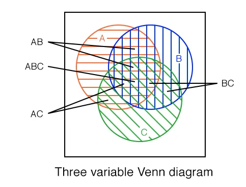
Let’s take a look at what the Boolean and operator does out in this Venn diagram here we’re going to kind of use these to showcase where the Boolean statements that we’re checking out with the Boolean operator where these statements are actually evaluated to be true. So if we assume that we are two facts here, A and B are both true. So let’s say this inner circle here, this left circle here represents a and this right circle here represents B and the square on the outside represents everything else. So when a and b are not, so if A and B are both true, then the statement evaluates to true. So the left hand side and the right hand side of the operator both must be true in order for the whole statement to be true. If A is false, or B is true. false, then the whole thing would be false. Now if we introduce a third fact, see, we kind of get the same results, right. So similar kind of story with the Venn diagram. Here we have a, b, and c. But notice that this little square here where we were actually filled in over here is no longer filled in. And that’s because all three facts must be true for the whole statement to evaluate to true. So a has to be true, B has to be true. And C has to be true in order for the whole statement to evaluate true.
So we’ll have similar representation here for the OR operator where the English word is the representation in Python of the OR operator the double bar symbol, so this is just the two vertical bars from your keyboard that is the OR operator in Java, C sharp and other programming languages and then a capital V is great. To be the OR operator for Boolean algebra. So let’s take a look at how or operates. So if we have the same statement, as we have before the same two premises A and B both being true initially, and the circles are kind of the representation of the same thing here, but the OR operator will evaluate to be true if either side of the operator are true. So if the left hand side is true, or the right hand side is true, the whole thing will be true. So if A is true, or B is true, so left hand side and the right hand side, so if A or B is true, then the whole statement is also true. And so nothing on the outside will actually be filled in quite yet. And the similar kind of story is for a third fact or fifth, that one has to be true for the whole statement to be true. So if any of them are true, the whole thing is true, but things kind of get tricky when we’re in introduce this next operator the exclusive OR exclusive or you won’t really find normally in programming languages. The Exclusive OR can be simulated using and or and the next operator that we’ll be covering here in just a second.
But the exclusive OR works in a little bit of a different way than the regular or the exclusive OR operates very similar to what we would expect the normal or operator to be in the sense that if A is true, or B is true, the statement is true, but notice that a and b is now false. If a and b are both true, the statement is false. So the exclusive OR operator is expecting one or the other. So that means the left side or the right side must be true, but not both. That is where the exclusive portion of the exclusive OR or the X or operator actually comes out. If I introduce a third fact things get to be a little bit more difficult to understand because now I would expect it to be kind of similar pattern as we have up here just to be, or on my just with my two facts, everything in the middle would be white, but everything on the outside would be red. But you notice when when we have all three to be true, all three can be true and the exclusive OR would still be true. Now let’s take a look at why that would be the case.
So let’s take a look at the example that we saw on the slides. We have our facts a, and our XOR operator. So we have a XOR B XOR. See, now if we kind of do our substitutions here now we could substitute ones and zeros here are true and false. So let’s go ahead and substitute our Boolean values here for our variables. So if A is true So we have a XOR B, which is also true. And C, which is also true. Now, just like most of your math problems, even when you’re just doing multiplication and division, you’re always going to evaluate your statement from the left to the right. So we need to first evaluates true x or true now XOR Exclusive OR exclusive right, the left or the right can be true, but not both. Since the left hand side of my operation is true, and the right hand side of my operator is true, this portion of the statement evaluates to false. Then all we need to do then is keep on working the rest of our statements. So we still have one XOR left. So we have false x or true? Now exclusive or one side or the other must be true but not both. So false x or true is actually true because both sides aren’t true. So this statement you say a false x or true, evaluates to true. So the whole thing true x our true, false XOR true, ends up being true.
So our last Boolean operator here is the NOT operator. The NOT operator acts pretty much like negation, as you would expect, like multiplying something by negative one not something is the opposite of what it actually is in Python as the previous Boolean operators the and and the OR operator, the NOT operator in Python is very English light not but Python is kind of weird. You will also see the exclamation point In some operations, but it doesn’t mean the traditional knots or negation operator as in many other programming languages. So, again, you’ll see not in Python, the exclamation point, this is going to be things like Java. And the weird sideways l here, this is going to be your Boolean algebra. So let’s take a look at what the Boolean operator not actually looks like. As I mentioned, the NOT operator is a negation, so not something as the opposite. So not a or not true is false. So not a if I write a here, so everything in the circle is a so when A is actually true, so everything inside of the circle then everything on the outside of a is actually true because it’s negated and similar idea for B when B is true, everything But B is true. So the whole statement is evaluated as such and similar idea if I introduce a third fact. So if I have three facts A, B and C, not B means that everything but B is true, just like in this example here.
So with all these new tools, we needed some new algebraic rules to really deal with them. Thankfully, most of the rules you know, apply quite well, but there’s one rule that needed to be added. In mathematics. When you multiply by negative one, you have to change the signs. Similarly, Augustus DeMorgan came up with a way to deal with the negation of entire Boolean logic statements. So this becomes very similar to how you multiply a statement or a regular mathematical statement by a negative one. I guess system marking came up with a way to deal with the negation of entire Boolean logic statements. The DeMorgan’s theorem essentially states to treat the NOT operator like the negative sign so you’re going to apply the negative to each of the premises or facts and then swap the operators or basically and become or’s and or’s become hands. So let’s take a look at an example. So if we invert our particular statement here where we have a and b, right, so A and B, not a and b becomes not a or not B, so we negated or applied the knot to a and the knots to b and the knot and becomes or similar idea for or not a or b becomes not a, and not B.
Now, in Boolean algebra, just like when you multiply by a negative one, a lot of the similar rules apply and Boolean algebra just like they do in mathematics. So in general, the OR operator works very much like the plus operator not works very much like negation, like we’ve already seen, and works very much like multiplication.
The associative property, also Hold. So we have a and b, and c becomes a and b and c. So if I made the substitutions here, just based off of what we had here, if we had one, and the AND operator works like multiplication, though times two, parentheses, substitute the multiplication symbol and for the end, and then we have three. That is the same thing as saying one times two times three.
The commutative property also holds. So again, let’s try to make some substitutions. A and B is the same thing as saying B and A. So that’s the same thing as saying. Two times three is the same thing as Three times two.
And the distributive property also holds. So A and B or C is the same thing as saying a and b, or a and c. So let’s make our substitutions again, let’s substitute again, one four a, so one times to remember, or is like the addition operator plus three is the same thing as saying, we’re going to kind of distribute right as we normally would with math, distribute the one across two plus three. So one times two plus three is the same thing as saying one times two, plus one times three. So we distributed the Want across and we’ll end up with the same exact result. Same idea or Boolean logic if we make each one of these properties, as we seen here, and mathematics applies and works directly with Boolean algebra. So what this really helps you as when you start working with Boolean logic, even when programming you can actually use these properties to simplify a lot of your Boolean logic statements to make them easier to read and easier to program.
With the new tools from Boole and DeMorgan, others began to see where they could be applied in the real world. In 1886, Charles Sanders Peirce noted in a letter that logical operations could be easily simulated by electrical switches. Many others worked on the idea too many to name here, but 51 years later.
In 1937, something happened. In 1937, Claude Shannon, a 21 year old graduate student at MIT was working on this same idea. He wrote a master’s thesis that some of called the most important master’s thesis of all time, titled a symbolic analysis of relay and switching circuits. In it, he showed that you could use electrical switches in Boolean algebra to construct circuits that could show any logical OR numerical relationship that you wanted. It’s available free online and will be linked in Canvas and linked in this video as well if you’re interested, but this is really cool. Kind of what was the gateway to electrical circuits, all of the cell phones and computers and electronic devices that you use today, this was the initial theory behind how all of those devices actually work.
So underneath Claude Shannon’s representation as far as translating Boolean algebra and Boolean logic into electrical circuits, we also needed a new representation for that this new representation is called logical gates. So it’s basically the same setup as we had with Boolean algebra and is very similar to if we have a and b, this is equivalent to this right where our two inputs are coming in on these two lines here are the AND operator it’s like a D, and then our output is the line leaving from the operator. similar idea for or so this is a or b we have XOR a XOR B, and not so this is same thing as saying that. Now really with the knot, the really important part is this little knot or this little mini circle at the end here and also note right that all of our Boolean operators here are compound operators, meaning that we have a left hand side and a right hand side, but the NOT operator only has one input. So one fact so just keep that in mind. But we can also apply the NOT operator to all of our other operators as well. So we can have NAND, nor, and x nor a little.at. The end here on the output is really the only part that matters for negating the result of a operation and and or XOR. One of the interesting things though, that it’s really kind of come out of the representation of Boolean logic on electrical circuits. So The work done by Claude Shannon and will continue part of this work and future lectures as well.
But one of the really interesting things that have kind of come out of this is the idea of a universal logic gate. The idea here is that any electrical circuit can be finished off by just using NAND gates. So all the complex Boolean logic that we could ever think of so any logical statements that we could write in Boolean algebra or Boolean logic can be redone with just using NAND gates or NAND operators, which is a pretty interesting thing and really why this is so important is that it greatly increases the speed efficiency and decreases the cost of manufacturing electrical parts.
Let’s go through an example of some Boolean logic now that we’ve covered some of the operators and some of the rules that govern the Boolean algebra behind it. A lot of times what you’ll see in computer science, especially when you’re dealing with Boolean logic and complex algorithms, our truth tables, truth tables showcase all the different options for each Boolean variable inside of a Boolean logic statement, as well as what output those particular facts for those variables actually produce. So let’s take a look at an example that we’ve already kind of done with end. So we’ve already explored the statement A and B, and C. You’ve already seen what the Venn diagram for that looks like, but we can also explore what that looks like again here in just a second, but let’s take a look at all possible values that we could actually input for A, B, and C. And if you remember, we’re only going to have two values binary values, either one, or zero or true or false. Now, both work synonymously. And you’ll find both in truth tables. And in fact, what the examples that you’ll be working with, we actually do use ones and zeros for true and false. So if you remember one means true, zero means false. But let’s take a look at how we can actually fill out our truth table here with those particular values. Now, I’m going to go ahead and use T for true and false. But as you could imagine, you could substitute one for true and zero for false and everything would be identical.
So what we would actually start with our truth table here as each of our columns here represent each of our variables or each of our facts as part of our Boolean logic statement though For a, what we’re actually going to do here, easy way to fill this out is we’re going to want to fill out all the different possibilities. So if we exhaustively go through each of our variables here, you may find that each one has two possible values. And then if we multiply this out, if it’s powers of two, we have eight possible outcomes or combinations of these values. You’ll notice that I have eight different rows in my truth table. That’s going to represent all of the different combinations that I actually have for this Boolean logic statement. Now generally, when we try to figure out how many different combinations we have the number of options we have for our variable to the power of the number of variables that we actually have, so that in this case would be two to the power of three. So two times, two times To write two times two is four times two is eight. This is the total number of possible combinations of truths or our facts that we actually could get out of this Boolean logic statement.
So let’s elaborate on that and fill out our truth table accordingly. The easiest way to start out for our truth table is go down one column first, because there’s kind of a general pattern that you can follow on filling this out. If we just fill half of our rows with false and then half of our rows with true we can work that out. So the column fills out pretty easily. This the pattern that you can kind of follow for the second column works as such, if you just fill in half of the falses, or half of the rows that was false of the first column with true and half of them with false and a similar pattern for the sets of trues down here. So if I make an imaginary line right here in the middle, we can try to fill out all the falses first. So, I want to fill out half of these with false and half of these with true. So let’s start with false first. So false, false, and then True, true. Down here, I’m going to do the same exact thing. false, false, true, true. And I’m going to continue the same pattern where I’m going to fill half of what I just filled in and see with falses, and half of what I just filled in with true. So for this set of falses, here, I’m going to have false true. With the set I’m going to have false true. Now, this pattern doesn’t exactly always hold, especially as you start adding a fourth column But with three variables, it’s pretty easy to fill out using this particular pattern. But if you find yourself filling out a truth table for more than three facts, all we’re actually doing is exhaustively writing out all of the different combinations of true and false values or each set of variables. Now, let’s go through and try to evaluate the output here, or our truth table. This particular statement is fairly easy with a and b, and c. Because we’ve already seen that with an and statement, both sides of the operator must be true for the whole statements to evaluate to true.
So in my output here, I’m going to write out what this set of facts this row of facts evaluates to for our Boolean logic statement up above. So I’m just going to kind of put row numbers here 123. And then let’s write our output. Over here, so, false and false and false, is going to evaluate to false because no sides are true and similar ID here, false and false is false. And true. is also False. False and true is False. False and False. False and true. And notice I’m evaluating this from left to right, right, because my statement is a and b, and c, so I’m evaluating the A and B first, and then I’m adding that result with C. So false and true is False. False and true is false. true and false is false, false and false is false. true and false is false, false and true is false. True and true is true. But true and false is false. True and true is true, true and true is true. Now on our truth table, we have a completed evaluation of what our Boolean logic statement A and B and C can actually cover, right, so we have all the different combinations of values, or truth of A, B, and C. And then we’ve also evaluated those truth values as part of our output. So now we know when this statement is true, and when the statement is false.
In lecture in the previous video, we saw what the AND operator looked like for our Venn diagram as well. So let’s kind of draw that over here, just so we kind of have what that looks like again, and or the statement just as we kind of had over in our truth table, we’re only going to fill in the spot where a true B is true and C is true, where essentially that means the output of our country table is true. So if I just kind of put a, b and c here, and then we also remember, we have a square on the outside that represents everything that is not A, B, or C. I will be giving you some more examples of this or where I’m going to actually give you the truth table, then you’re going to try to generate the Boolean logic statement and the Venn diagram and even some logic gates.
But let’s try to draw the logic gates for this as well. And the examples that you’ll be doing our logic gates are written like this. So we have our three inputs A, B, and C. Now if you remember the logic gate for and looks like this. Let’s draw that. So what we want to do is start out by drawing the logic gate for the first part. Have the logical statement, which is a and b. So to do that, you can kind of imagine electrical wires kind of coming off of the sources of A and B, or your individual variable. So I’m going to draw kind of a little wire out over here into my open space on the right from a and then my second input to that statement is B. So I’m going to draw a wire out from there. And I’m going to draw my gate. So it looks like a D, and my output there. Now I can draw the second part of the statement, which is and C. So I’m going to draw a line from C and draw out here and it’s okay if your wires go at a 90 degree angle or a little bit of a curved connect the logic gates together. And now that I have the output from a and b, and the output the input from C, we’re going to join those together with another and gate. So the logic gate drawing of a and b and c can be viewed as that. Now everything that I just did apart from generating your truth table are going to be reviewed and practice in a few examples.
In this video, Carrie Anne shares the principals of binary numbers and how we use Boolean Algebra to work with binary values. We get to see the truth tables for the basic statements (or, and, not, xor) as well as their respective logic gates. We also get a good primer for working on more complex statements.
CrashCourse. “Boolean Logic & Logic Gates: Crash Course Computer Science #3 “. Mar, 8, 2017. YouTube. Available: https://www.youtube.com/watch?v=gI-qXk7XojA
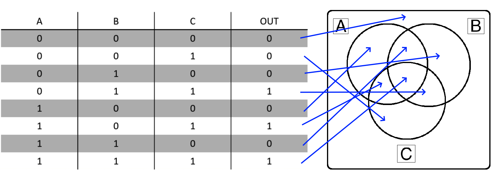
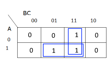
So let’s take a look at example one. And the best way to start this is where the output is actually true. So if we examine this line here, this line and this line, we can see that when B and C are true, output is True. When a and c are true, the output is True, or when all three are true, the output is also true. So a really good way to start is just by coloring in these three facts.
So when B and C are true, that’s this little square here. Then when a and c are true, that’s this little portion of the Venn diagram. And then when a, b, and c are so when all three are true, And that’s this little center part of the diagram. And then all other rows of the truth table are all false or zero. So we’re not going to fill in anything else in the Venn diagram here. So this is the full output of or the full expression represented as a Venn diagram.
So let’s tackle this as a Boolean expression. And so we’ve already talked through parts of what the Boolean expression would actually be. So this can start here with a and c, when a and c are true, the statement is true. So let’s write a and see us as one portion of our Boolean expression. So I’m going to write that using parentheses, and then we have B and C. So I’m going to kind of write this over here, B and C. What that’s the other part of the truth in our Boolean expression, but we can’t just write them side by side, right, we need to join the middle because we also need the center portion. So it’s either a and c are true, or either A and C or B and C. So enter a or operate in between. So if A and C are true, or B and C are true, so that’s this portion right here. So when a and c, or B and C are true, and our expression is true, this will represent our Boolean logical statement. But there are alternative ways to write this. And these aren’t just the only ways another way you could have wrote this would be C, right? Because in all three cases, C is always true. So C, and a or b.
So let’s take a look at what the logic gates look like. So the logic gates and I’m going to write the logic gates for my top statement here. So this one right here, we need to write the left and right hand side of the OR operator first, and the OR operator is going to join these two at the end. The lines here represent the inputs of A, B and C. So I’m going to draw out the input of a because in this case, we have a and c. And those are connected together with the AND operator. And that gives an output and we have the same thing with B and C. So we have B, C, those are both connected together with an AND operator and both of those are joined together using or. So this would be the logic gate for this particular statement here.
Let’s do a bit of a deeper dive into that worked example to explain some of the nuances working with Boolean Logic Expressions, Truth Tables, Venn Diagrams, and the connections between those three. Unfortunately, this is not well explained or covered elsewhere in online resources, but we find that it is really helpful to revisit these concepts here before the end of this module.
This is a lot of conceptual information to digest at once. However, we don’t expect you to become proficient in this right away! This is just meant to be an introduction to the concept of Boolean Logic and Boolean Algebra, which you’ll become more comfortable with over time as you practice your programming skills and take later classes in Computer Science.
For now, we just want to introduce the topic and give you a chance to try it out in the quiz at the end of this module. If you don’t do well on the quiz, don’t sweat it!
This material is handy if you want to review the concepts or get in some practice, but the best way to learn is to just keep doing examples and practicing as you learn to code.
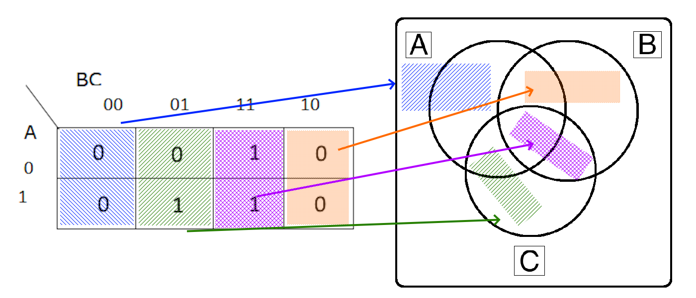
When working with Truth Tables and Venn Diagrams, the key idea to remember is that each line in the Truth Table corresponds to exactly one space in the Venn Diagram.
Each labelled section in the Venn Diagram above corresponds to the variables that are True or 1 in the corresponding Truth Table. We can even draw arrows directly from each line in the Truth Table for Example 1 to the Venn Diagram:
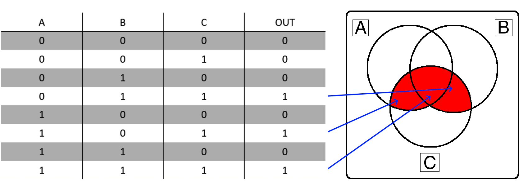
So, if the “OUT” column in the truth table is True or 1, that section of the Venn Diagram becomes shaded and is part of the desired output. Therefore, if you have a Venn Diagram or Truth Table, the conversion between the two is a direct one-to-one connection. Here’s what that looks like for Example 1:
Once we understand either the Truth Table or Venn Diagram for a desired Boolean Logic expression, we can use that information to start building the Boolean Logic expression itself. This can be done in one of three ways:
So, let’s go through these three methods and see how they relate.
Let’s start by directly converting the information in our Truth Table and Venn Diagram to individual Boolean Logic terms. To do this, look at each row in the Venn Diagram where the “OUT” column is 1. Then, for each variable in that row, we either include it in the term directly if it is a True or 1 in the input, or else we include it with a NOT symbol ($\neg$) before the variable if it is a False or 0 in the input. We must include these false variables in our terms, or else we would get different results (i.e. $A \wedge B$ is not the same as $A \wedge B \wedge \neg C$)
So, we would end up with these three terms from our truth table above:
Finally, our full Boolean Expression using these three terms would combine them using the OR ($\vee$) symbol. This is because the “OUT” column in the Truth Table is True or 1 if any one or more of these terms are True. So, our resulting Boolean Expression at this point would be the following:
$$ (\neg A \wedge B \wedge C) \vee (A \wedge \neg B \wedge C) \vee (A \wedge B \wedge C) $$
At this point, we can stop if we don’t care about reducing the expression to simpler terms. So, once again, there is a direct one-to-one translation from either a Truth Table or Venn Diagram to a Boolean Logic expression that is in this form. In fact, this form is known as the Disjunctive Normal Form of a Boolean Logic expression (though it is not the reduced form). A great way to remember this form is that it is an OR of ANDs (the individual terms are all AND operators, and then the terms are combined using OR operators).
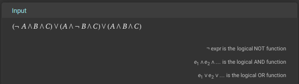
Before we go any further, we can check our work by entering this formula into Wolfram Alpha and checking the Venn Diagram and Truth Table it produces and make sure they match our original setup. While it is possible to enter all of the fancy Boolean Logic symbols into Wolfram Alpha (it does understand them), it is often easiest to just convert them to their English counterparts as shown below:
(NOT A AND B AND C) OR (A AND NOT B AND C) OR (A AND B AND C)You can also click this link to go directly to Wolfram Alpha with this input provided.
First, we can check that our input is parsed correctly since it matches our Boolean Logic expression at the top:
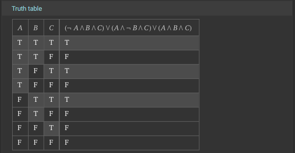
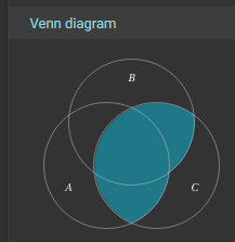
We can also look at the Truth Table and Venn Diagrams further down:
Notice that the Truth Table is ordered a bit differently than what we see above (it is reversed), and the Venn Diagram is rotated a bit, but hopefully it becomes pretty clear that we have a match! So, our translation from the Truth Table to a Boolean Logic Expression is valid!
Once we have a valid Boolean Logic Expression, we can use the laws of Boolean Algebra to reduce it. We cover some of these laws earlier in this chapter, but Wikipedia has a good listing of them as well. We’ll refer to the laws as they are described in Wikipedia as we perform these operations.
First, it is often very helpful to remember that, in many cases, AND ($\wedge$) can be treated similar to multiplication ($\times$), while OR ($\vee$) can be treated like addition ($+$). So, in some fields (such as computer engineering), it is common to rewrite the statement above like this:
$$ (\neg A B C) \vee (A \neg B C) \vee (A B C) $$
This may make some operations more intuitive, especially where we are “factoring out” or “distributing” a term by applying the Distributivity laws. So, we’ll use this modified notation while performing our Boolean Algebra reductions.
Unfortunately, reducing this expression is actually a bit complex, because there is not an obvious starting place. Instead, what we need to do first is duplicate a term by applying the inverse of the Idempotence of $\vee$ law. This law states that $ x \vee x = x $, so we can invert it by replacing any single term $x$ with two instances of the term that are connected with the OR ($\vee$) operator. We’ll do this to the last term in the expression for now:
$$ (\neg A B C) \vee (A \neg B C) \vee (A B C) \vee (A B C) $$
Next, we want to group some similar terms together to make later operations a bit more obvious. So, we’ll apply the Commutativity of $\vee$ law to rearrange the terms, and also use the Associativity of $\vee$ law to group some terms together:
$$ \Big( (\neg A B C) \vee (A B C) \Big) \vee \Big( (A \neg B C)\vee (A B C) \Big) $$
Now we can start to simplify things a bit. In both groups of terms, we notice that they each share the variable $C$, so we can apply the inverse of the Distributivity of $\wedge$ over $\vee$ law to “factor out” that term. Notice that this is very similar to how we can apply a similar law in ordinary algebra:
$$ \Big( C \wedge \big((\neg A B) \vee (A B) \big) \Big) \vee \Big( C \wedge \big( (A \neg B)\vee (A B) \big) \Big) $$
After that, we’ll see that the first pair of remaining terms shares the variable B, while the second pair of terms shares the variable A. So, we can once again apply the Distributivity of $\wedge$ over $\vee$ law to “factor out” those shared terms in each pair:
$$ \Big( C \wedge \big(B \wedge (\neg A \vee A) \big) \Big) \vee \Big( C \wedge \big(A \wedge (\neg B \vee B) \big) \Big) $$
Now we can start to remove some terms. The Complementation 2 law in Wikipedia states that $x \vee \neg x = 1$, which means that we can replace a term and the inverse of that term connected with an OR ($\vee$) operator with the value True or 1. We’ll do this for both $A$ and $B$ terms:
$$ \Big( C \wedge \big(B \wedge 1 \big) \Big) \vee \Big( C \wedge \big(A \wedge 1 \big) \Big) $$
Next, we can use the Identity for $\wedge$ law, which states that $x \wedge 1 = x$, to effectively remove those True or 1 terms from the statement. Again, remember that in regular algebra, we would know that the term $1A$ would be equivalent to just $A$, so if we rewrite $A \wedge 1$ as just $1A$ and then just $A$, it feels very logical!
$$ ( C B ) \vee ( C A ) $$
Finally, if desired, we can apply the Distributivity of $\wedge$ over $\vee$ law one more time to “factor out” the $C$ variable again:
$$ C \wedge (B \vee A) $$
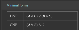
There we go! Both of those reductions are valid minimal forms of the Boolean Logic Expression. Once again, we can go back to Wolfram Alpha to check our work:
In that screenshot, we can see both the minimal Disjunctive Normal Form (DNF) as well as the minimal Conjunctive Normal Form (CNF) for the expression.
Another great way to convert a Truth Table or Venn Diagram into a Boolean Logic Expression is to use a bit of intuition. The video earlier in this chapter showed one way to do this suing the Venn Diagram, but let’s use another method - using a concrete example!
For this example, let’s assume that we have been given the following rules:
We can build a Truth Table using these rules as shown below:
| Friends Over (A) | Sunny Outside (B) | Mom Says Yes (C) | Go Swimming |
|---|---|---|---|
| 0 | 0 | 0 | 0 |
| 0 | 0 | 1 | 0 |
| 0 | 1 | 0 | 0 |
| 0 | 1 | 1 | 1 |
| 1 | 0 | 0 | 0 |
| 1 | 0 | 1 | 1 |
| 1 | 1 | 0 | 0 |
| 1 | 1 | 1 | 1 |
Ahh! Notice that this Truth Table is identical to the Truth Table given in Example 1 shown above! We have created a set of rules that immediately generate the same Boolean Logic Expression that matches our example. It may take a little bit of thinking, and we have to state the rules very clearly, but generally we can always create a set of rules that clearly describe any Truth Table. In practice, we often are starting with a set of rules like this (in our specifications document), and we are trying to build a Boolean Logic Expression that we can use in our code as we implement those specifications in our program.
Now, let’s use a bit of intuition about those rules above to generate a Boolean Logic Expression. If we really want to go swimming, we’ll quickly realize that there are two main things that we need to have:
Look closely at those rules! Just by talking through the scenario, we have created a Boolean Logic expression. Let’s rewrite it:
Mom must say yes
AND(it must be sunny outsideORwe have to have friends over)
If we replace each part with the corresponding variable, we can find the corresponding statement:
$$ C \wedge (B \vee A) $$
A similar way to state the rules might be:
Once again, we can rewrite that a bit to make the Boolean Logic operators more obvious:
(Mom must say yes
ANDit must be sunny outside)OR(Mom must say yesANDwe have to have friends over)
Finally, we can replace those parts with variables to get the corresponding statement:
$$ (C \vee B) \wedge (C \vee A) $$
So, as we can see, applying a bit of intuition to a real-world example that creates the same situation can make it pretty easy to work out a simple Boolean Logic Expression from a Truth Table or Venn Diagram.
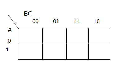
The third method would be to use a Karnaugh Map. We won’t go into this method in too much depth, but we’ll briefly show how it works. There are some great online resources to learn more about applying Karnaugh Maps in this context.
First, we’ll start with a blank 3 variable Karnaugh map. A Karnaugh Map is essentially a different way to structure a truth table by placing similar entries next to each other in a particular way:
Then, we’ll input the desired outputs from the Truth Table in each square of the Karnaugh Map:
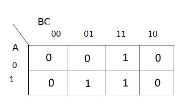
Now, we’ll group connected terms. These groups can be either rectangular or square boxes. So, for this Karnaugh Map, there are two groups:
Finally, for each group, we identify the variables that don’t change within that group, and those become our terms. So, for the group in the bottom row, we see that both $A$ and $C$ are the same, but $B$ changes. So, one term we find is $AC$. For the group in the third column, we see that $B$ and $C$ are the same, but $A$ changes, so our other term is $BC$. Then, we combine those two terms together using the OR ($\vee$) operator to get this statement:
$$ (AC) \vee (BC) $$
There we go! That is once again one of our minimal Boolean Logic expressions found earlier.
Once clever things that we might notice is that there is also a one-to-one equivalence between Karnaugh Maps and Venn Diagrams. We know this since there is already a one-to-one equivalence between both of those and the original Truth Tables, so it is an easy assumption to make.
So, we can quickly see the arrangement of items in a Karnaugh Map and how they match up to our Venn Diagrams as shown below:
Notice that the the Venn Diagram has a very similar layout to the Karnaugh Map. This is because both of them are structured in a way for similar entries to be near each other. In fact, each time you cross over a line in a Venn Diagram, only a single variable changes value. The same works for a Karnaugh Map.
So, with a little intuition and an understanding how Karnaugh Maps work, we can perform a similar analysis directly on the Venn Diagram itself.
Why does all of this matter? Well, when we are trying to convert a real-world situation to code, it is often helpful (but not necessary) to be able to reduce our Boolean Logic expressions to simpler terms.
Let’s go back to the concrete example shown above. If we wanted to write a Python program for this, there are a few ways we could build it.
First, here’s what it would look like if we just directly encoded the rules as written:
# bool() returns False if the input is the number 0, otherwise True
# so we have to convert the string to an int first
sunny = bool(int(input("Is it sunny outside? (1 = yes, 0 = no)")))
friends = bool(int(input("Do you have friends over? (1 = yes, 0 = no)")))
mom = bool(int(input("Did Mom say yes? (1 = yes, 0 = no)")))

"""
Rules:
* If Mom says yes and it is sunny outside, we can go swimming even if we don't have friends over.
* If Mom says yes and we have friends over, we can go swimming even if it isn't sunny outside.
* If Mom says yes, we can go swimming if it is sunny outside and we have friends over.
"""

if (mom and sunny and not friends)
  or (mom and friends and not sunny)
  or (mom and friends and sunny):
    print("We can go swimming")
else:
    print("We cannot go swimming")
We could also use if-else statements instead of the or operator to achieve a similar effect:
if mom and sunny and not friends:
  print("We can go swimming")
else if mom and friends and not sunny:
  print("We can go swimming")
else if mom and friends and sunny:
  print("We can go swimming")
else:
  print("We cannot go swimming")
However, in both cases, these programs are more complex than they actually need to be, and it may make things more difficult to debug down the road. So, with a little intuition and the ability to reduce Boolean Logic expressions effectively (and correctly), we can simplify this code quite a bit:
if mom and (sunny or friends):
  print("We can go swimming")
else:
  print("We cannot go swimming")
Hopefully you can see the value in that much simpler program, both in terms of how easy it is to understand and debug, but possibly how much more efficient it is overall since it has fewer comparison to make.
Image Source: https://www.allaboutcircuits.com/textbook/digital/chpt-8/boolean-relationships-on-venn-diagrams/ ↩︎
Image Source: https://www.wolframalpha.com/input?i=%28NOT+A+AND+B+AND+C%29+OR+%28A+AND+NOT+B+AND+C%29+OR+%28A+AND+B+AND+C%29 ↩︎ ↩︎ ↩︎ ↩︎
Image source: https://www.learnelectronicswithme.com/2021/09/karnaugh-map-and-steps-to-solve.html ↩︎
Read Pattern on the Stone, Chapter 2.
“The Pattern on the Stone: The Simple Ideas that Make Computers Work” by W. Daniel Hillis. ISBN 046502596X, newer version is also available and will work fine

In this video, we’re going to take a look at computer programming languages and some of the history that’s behind them. First off, what exactly is a language. Something that we don’t really think about very often though. A language really is just a set of symbols, whether it be gestures, words, sign language, or even Braille, that are used in a uniform fashion to allow people to communicate with one another. We have to take a look at how we as humans can communicate with a physical or inanimate object: a computer. In order for us to tell computers what to do, we had to develop a language that we could use to communicate with it. Here on my slide I have on the left a bunch of different ways on how to say good morning, in various human languages that we use to communicate with with one another. And on the right side here we have a bunch of computer languages that we have. So the first one up here is happens to be Python 2, Python 3, C, Java, JavaScript, and even Rust. And so this is just a small number of different things that we would be able to use to communicate this particular message to our computer. Just likewise, we have a lot of different ways we could say good morning to someone.
Let’s take a look though on where the idea of a computer language actually started to originate from. Ada Lovelace is our first influential woman in computer science that we’ll talk about. She is regarded as one of the first figures in history to truly understand computer programming, possibly only second to Charles Babbage. Ada Lovelace was the daughter of a famous English poet. Lord Byron, who I’m sure you’ve heard about before, but she had very little contact with her dad pretty much at all, and during her childhood, she was pretty much on her own. But during that period due to her father status, she was tutored by some of the greatest mathematicians of that time, including Augustus de Morgan, remember from the Boolean logic lecture, had the De Morgan’s theorem. And so she was already being tutored by some of these great mathematicians who were laying the groundwork and the foundations for what we use in computer science. One of the… one of the greatest quotes from from Charles Babbage, who he was talking about Ada Lovelace with. So, Charles Babbage said that Ada Lovelace was that “Enchantress who was thrown her magical spell around the most abstract of sciences and has grasped it with a force few masculine intellects could ever have exerted over it.” So this is a really big compliment from Charles Babbage, who was pretty much the pioneer in computer science at the time.
Ada Lovelace spent a lot of time visiting Charles Babbage and she was so intrigued by his Difference Engine that he had in his house, the prototype that he had made. But her goal in visiting with Charles Babbage so much is that she started to translate his work into English so she could bring it back to England, and explain how it worked and why it was so important and revolutionary. And to assist with that she included a set of notes with her own descriptions of the design of his Difference and Analytical Engines and how they actually worked and when completed her notes are actually longer than Charles Babbage’s memoir. She has so she had a very deep understanding on how Charles Babbage’s machines actually work.
What makes Ada Lovelace so unique in the history of computing is Section G here in her notes. in that section she describes in complete and utter detail how you would use Babbage’s analytical engine to calculate a sequence of numbers called the Bernoulli numbers. You’re probably also familiar with. But while it appears to be written in English, it’s actually designed in a way that can be directly used by the Analytical Engine. So, in a way, you could say that it is in a language that the analytical engine would understand. And in doing so, she wrote the first computer program, which is simply, right, a series of steps specifically designed in such a way that could be easily ran on a computer.
There is some debate as to whether or not she wrote some of the programs she was previously attributed to. But there’s little doubt in the fact that she would be capable of doing so. In fact, she was one of the few people who saw the true potential of what Babbage had actually created. And she’d once remarked that under the correct circumstances, it could be used to create music. So the Analytical Engine she was talking about here. And that’s really quite extraordinary, something that Babbage probably hadn’t thought of at the time. But if you are a musicphile at all, music, right is just simple mathematics. And so if you have a machine that can compute mathematical values, why wouldn’t it be used to create music? So all told, Ada Lovelace is really truly a very important person in the history of computing science. And she’s widely regarded as the world’s first true computer programmer. And as a as another bonus side note here, she’s actually credited with discovering the first bug in a computer program as well. A bug. In fact that was found in a program that was written by Charles Babbage.
Our next famous woman in computer science that we’ll be talking about is Rear Admiral Grace Hopper. Grace Hopper enlisted in the Navy and worked on the Harvard Mark I computer, as well as the UNIVAC, a successor to the ENIAC, and we’ll talk about the UNIVAC and ENIAC computers in another lecture. So grace also developed a programming language called FlowMatic which was later adapted into a language called COBOL, which is still somewhat used today. COBOL is traditionally a language that was used very heavily in the financial industry, because it was used to generate a lot of financial reports. You don’t see it a whole lot now, you may see it used occasionally at places like banks, or accounting firms and things like that, but it’s not very widely used anymore.
But beyond that, she was a truly a pioneer and out of the box thinker for her entire life. And as you’ll see in the following videos, Grace Hopper is a pretty sassy lady but a pioneer in modern computing. She was also pretty famous for her description of a nanosecond in the Dave letterman show, which you’ll see here in just a little bit. Another thing here every year, there is a Grace Hopper conference to celebrate diversity and inclusion and women in computing. And so there’s actually scholarships available for students if you would like to attend this conference. And it’s something that I would highly recommend if you ever get the chance, it is truly a great experience to actually participate in.
YouTube VideoDue to the privacy settings, we were not able to embed the following video directly.
Discussion of a nanosecond starts at 4:17
YouTube VideoThe next influential woman in computer science that we’ll talk about here is Margaret Hamilton. Margaret was the director of software engineering at MIT’s instrumentation lab. Margaret Hamilton was also known as the, essentially the creator of the field of software engineering, essentially. But the reason why she is credited for software engineering is that she was responsible for a team that developed onboard flight software for the Apollo space program. During this timeframe, her program actually prevented a mission abort during the Apollo 11 moon landing, which is kind of crazy cool to think about right.
In this picture here is, she’s actually standing next to the output of one of the programs that they had actually made. In the video here you’ll see that, you know, programming at this time was completely by the seat of your pants, right? There was no really step by step procedure or best practice of programming pretty much anything. And so the idea that NASA trusted this group of engineers to create the flight software for the Apollo space program was really kind of crazy to think about. And so if you had actually messed up, right, the output of your program would just be you know, feet high instead of just a few pages long, which is this famous picture with Margaret Hamilton here in the slide.
So what really is programming? Right? We’ve talked about a lot of famous women in computer science so far, that have been very influential; the first computer programmer Ada Lovelace, the queen of software Grace Hopper, and Margaret Hamilton, who really pioneered the idea of software engineering, best practices with computer programming. But, what does that really actually entail? Well, programming itself, right computer programming, is simply the act of designing, writing, debugging and maintaining the source code of a computer program.
Let’s imagine that we’re writing a program, a very simple program, that takes input from the user, and then prints out a result that is divided by 61. So the user inputs a number and then we divide it by 61 and output it. So what would that program actually look like? Well, in Scratch, right, it would look something like this. This programming language is very English like, right? It’s a block based programming language that is designed to teach young kids, even up through middle school on basically how to program. And it makes it a lot easier for humans to understand. Because even if I showed this to my grandma, she could probably deduce kind of what’s going on here. Ask for a number and wait, and then divide whatever the answer to that question was by 61. And stop, right? Simple enough. So, very easy for a human to understand.
But do you really think that a computer is able to understand this language? Probably not, right? My computer has no idea what the idea of a block is, right? Computers really only only care about ones and zeros. That’s it. So how do we get from a block down to something a computer can actually understand? So that’s really going to highlight our language hierarchy here. So our high level languages, so the stuff that humans can understand, so stuff that we can understand is what we pretty much deal with on a daily basis as computer scientists. But, then we can kind of go down our stack right into the assembly, machine code, and then down on the hardware, where the actual physical hardware could actually interpret what we’re trying to talk about. But first off, let’s take a look at more high level languages.
So we’ve already showcased Scratch, which is a very human readable. But here is a program written in C or C++. And we’re now starting to get into some stuff that is not so human readable. This in general requires a little bit of training in order to understand, right? Just like if you don’t know Spanish or French, if you are trying to read something in that, in that different language, you need a little bit of training to figure out what was going on. So we have a lot of extra syntax here like printf, right? What does that mean? What is a float? If I, if this is the first time ever reading a programming language, I’d have no idea what some of these things actually are. But again, right, this is the same program: input a number divide it by 61. And then output that result.
Same thing goes with Java, right? As you can see here, we have a lot more, a lot more fluff, right. So we have a bunch of import statements up here. We have we now have to have a class and we have to have a public static void main string args, whatever the heck that’s supposed to mean, right? And even beginner Java programmers aren’t even introduced to this concept until once you get deeper into that particular course, What’s a scanner? What are we scanning? I don’t know. So again, right requires a little bit of extra training and Java, with it being an object oriented programming language, adds a lot more fluff and syntax and wrapping to our program just for a simple program like this in order for it to work.
And C# isn’t much better. C# is essentially Microsoft’s flavor of Java, but does the same thing right: inputs a number, divides by 61 and outputs it. I would argue that this code here is a little bit easier to understand. But again, right, we have a bunch of extra fluff here that you know, start from scratch is a little bit more difficult to understand without a little extra training.
Now Python, like Scratch, is generally touted very human readable. So it doesn’t have all of that extra fluff, right? We have no class, or namespace or inputs, or sorry, imports to define here. We just take input, and then convert it to an int, store it and then print out the result, right? Simple enough. So all of this extra fluff that we had here, in C#, I’ve reduced all of this down to two lines in Python. That’s why Python is traditionally used as a scientific language because it’s a lot more accessible to non-computer scientists.
But again, right, there’s tons of different programming languages out there and they all have their purpose. They all have their place. Some more human readable than others, right? We’ve talked about COBOL already right with Grace Hopper, Pascal, Visual Basic Perl, fortran which is an old one as well. Basic is another older programming language. There’s way too many of them to list here. But the point is we have a lot of different languages with the various different purposes, but all of them with a trained computer programmer, could use them to communicate their particular idea or task or whatever they’re trying to do to the computer. But again, right, all of those languages can’t be understood by the computer directly.
The majority of those languages will have then a compiler associated with them. And compiler or assembly is typically a language that is assembly language is typically still readable by humans, but is much closer to the language a computer would actually understand. And assembly language requires much more training to actually understand what’s going on. And so to go from a high level language to assembly language, we’ll use a program called a compiler, which in its entire purpose is to act as a translator. So the language that we use to write our program and like Python, or Java, let’s say, is then compiled and translated down into an assembly language, which is closer to what the computer can understand. Here’s our C program, the assembly language that’s associated with that after it’s been compiled. This particular part is simply, right, taking a number and dividing it by 61. And this is, this is a heck of a lot more complex, isn’t it? Right? You will eventually, or if you, if you take some of our upper level computer science courses, you will learn how to translate all of this and understand what’s going on here. But the majority of computer scientists aren’t going to need to understand assembly language unless you’re dealing more with things at the operating system level or hardware level and things like that, or even cybersecurity if you’re into cybersecurity, being able to understand some assembly is quite useful. Not directly interpretable by your hardware quite yet.
Once we have our assembly language that is going to be then fed into the assembler, the assembler is going to take the assembly language and convert it into machine code, which is then directly read by your computer. The assembly and things like that. Some of this will actually depend on the operating system, the architecture and things like that, that you’re actually running on your computer. While the high level language is uniform, mostly across all machines, the assembly code is not. Likewise, machine language is very specific to the machine that it’s being built for. So, machine language is just simply a set of binary code, all ones and zeros, that tell the computer exactly what to do. And so here’s the machine code for the assembly language that we just saw previously. Theoretically, right? You could translate all these ones and zeros back into the original program. But that’s pretty difficult to do, right? It requires a significant amount of training to be able to try to translate these ones and zeros back into what it was originally.
And so now we’re getting into code that can be interpreted directly by your machines, hardware. Your hardware, really all it cares about is current or no current, right? Electricity is on or the electricity is off. And so this simply refers to the structure of chips and circuits that your computer is made of. And we’ll talk more about that in another lecture. But, and the gist of it here, right, we’re feeding all of our ones and zeros into each of the inputs of our hardware, which is taking those ones and zeros, doing some sort of calculation and outputting the result back to your computer.
But overall, right this is kind of the big picture of computer programming, right? We go from a high level language, where we have things like Python, C, C#, Java, JavaScript, all of those languages that you would normally program in, as a, as a software engineer. And those languages are then compiled or taken by a compiler and compiled into assembly language, which is more machine specific, right, depending on operating system, Mac, Apple, Linux, that sort of thing. 64 bit versus 32 bit processor, lots of different things that go into that particular compilation. But that assembly language is then assembled, taken by the assembler and then converted into machine language which is just the ones and zeros that your hardware is going to interpret
Read Pattern on the Stone, Chapter 3.
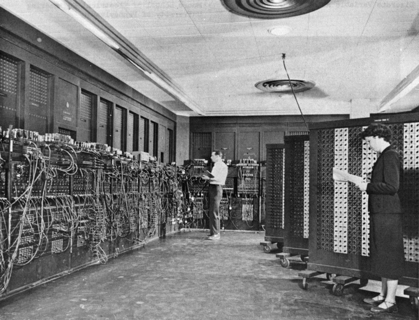
Welcome back, everyone. In today’s video, we’re going to be talking about universal computers. Now to pretty much pick up where we left off a while ago when we were talking about Boolean logic, Claude Shannon had just proposed a way to take electrical circuits and represent any Boolean logical statement with them. And so this was a huge turning point in the history of computer science. But how did we make the leap from Boolean logic on electrical circuits to the modern computers that we have today, and we’ll talk a little bit about that gap here today, but there will still be some missing parts that we’ll talk about later. But this brings us to Herman Hollerith, who at the time was a United States Census office employee, and he was tasked with coming up with a better way to calculate the census result. Because at the time, calculating the US census was incredibly slow. The 1880 census alone took eight years to tabulate, which really kind of defeats the purpose of a census, right? If you only know how many people you have in your country, eight years after the fact, the census was actually taken.
And so 10 years later, Herman had actually implemented a new system. And so in 1890, when he tabulated the US Census, then it only took one year to complete versus the eight years from the 1880 census. And this is even taking into account the 30% increase in population over that decade, which is pretty impressive, to say the least. So how did he do it? Well, just as Joseph Marie Jacquard had discovered, punch cards are really great way to organize and calculate information, particularly when you want that information to be read and used by machines. And so Hollerith was inspired by this fact. But really, actually, he was inspired by the way railroad conductors would actually use punch cards to track the gender and age and so forth from people buying tickets for the railroad. So not only did Herman Hollerith develop a new punch card in order to track US Census data, he also developed a machine to actually read it.
So this is an example of a Hollerith tabulating machine that was used in the 1890 census. So this machine could read the card and tabulate all of the information that was on them, and was also advanced enough to actually infer other facts and keep track of things like the number of married men and women. And depending on the data on the card, there is a compartment down you can kind of see towards the bottom right hand corner there. That was a storage box, for the cards and so depending on what kind of data was actually on the cards, a compartment in this storage box would open. So the operator that was using the machine could take the card from the machine and put it in the corresponding box. So essentially right it was auto sorting all of the census data, which was also pretty cool. But Hollerith continued to improve his designs and created several upgraded machines that could tabulate all sorts of data, not just census and donation, he would go on to create his own company, the Tabulating Machine Company, and a couple decades later, his company would join several under under a new name the Computing Tabulating Recording Company. But this was eventually renamed to be something else, the International Business Machines company, right. And many of you all know this company as IBM. Pretty cool, right?
This is something that I learned when coming to computer science, I had no idea how IBM got their start, but tabulating machines is pretty much where they come from. Now, this particular image from this slide is from the US Social Security Administration in 1936. This shows several IBM tabulating and sorting machines in use. And so they use these for all sorts of things as time progressed, and each one was able to keep track of all sorts of different kinds of information. One example could be tracking the sales of a particular person or company for the purpose of billing, right, or tabulating sales, and inside of a convenience store or something like that. Does all sorts of things, right. So things that were traditionally done on pen and paper or pencil and paper, and prone to a lot of human error. We could feed these punch cards through these machines and they would auto tabulate everything. For us, and they were pretty popular all the way through the 50s and 60s, until the computer started to take over really, but this pretty long time, right? About 30 years or so, for these tabulating machines, as they kind of took their grip. But we’ll talk a little bit here in just a second about the actual first computers that we actually had in the United States. But just as a quick little fun fact, we’ve talked briefly in a previous video How pretty much took a country torn by war before we actually started, or the world torn by war, really. Before we started to get a lot of advancements in computing technology. IBM was actually involved with selling these tabulating machines to the Nazi Party in Germany and may have inadvertently aided their attempts to catalog and later persecute the Jews. During the Holocaust, so a little bit of dark history behind IBM and their tabulating machines.
But anyways, let’s talk about the some of the early major computers that we actually had in the US. So, first and foremost, the mark one, the mark one that was really important because we started to see a shift from pure mechanical computers or computers like tabulating machines to something that was a little bit more flexible, a little bit more powerful, as far as what type calculations that could be done. But the mark one was an electromechanical computer, and it was the largest of its type ever built. And its main purpose was actually to aid in the calculating ballistics tables that were needed by the gunners to accurately aim and fire weapons that were being developed for the war because to try to stay ahead, the US was developing weapon at an alarming rate. And the time it would take about 20 hours for a skilled mathematician to analyze a single 60 second trajectory shot. This is way too slow at the pace that weapons are actually being developed. And so the mark one was completed 13 years after it was commissioned in 1944. And proved to be pretty useful, right. So this is also remember back with Grace Hopper when we talked about her. This was the computer that she was commissioned to work on by the US Navy. So then let’s chat about the kind of the next step up right. So the mark one was an electro mechanical computer, which had tons of parts, right. Five tons of computer if you can imagine that. And one little But the fun fact that I always like to emphasize here is that the mark one had five horsepower. Right? So it actually had an engine their in order to run it. So if you can kind of imagine having a laptop that had an engine in order for it to actually work kind of crazy to think about that your computer has horsepower.
But we did take a big leap forward after the mark one was completed. So in 1943, the US Army and the University of Pennsylvania began working on a project that would be the successor to the mark one called the electrical numerical integrator and calculator or any ENIAC right. Scientists like acronyms, and sometimes they’re pretty good. Sometimes they’re not so great. But when the ENIAC was completed in 1946, it turned out to be about 1000 times faster than the mark one. But the ENIAC was so revolutionary. because it was the first all electric programmable computer that was truly general purpose. And we’ll talk about that here in just a little bit. But remember how we were talking about the Difference Engine that Charles Babbage created that was truly are the Difference Engine number two in the analytical engine that were truly general purpose computers, right. And so now we have the first all electric computer compared to the mark one, which still had a lot of the mechanical parts right had five horsepower. But the ENIAC ran almost continuously from 1946 to 1955. So had a pretty good long, long term operation here. Again, right had an insane number of parts right over 17,000 vacuum tubes that were used to run at 70,000 resistors, 10,000, capacitors and over 5 million hand soldered joints. If you have a hard time trying to figure out what’s wrong with your computer Now, imagine trying to debug and fix a computer that had so many different moving parts or so many different hand soldered parts is really kind of crazy to think about. But we’ll bring up the neck and the mark one and another lecture as well.
But I do kind of want to highlight a really big important part during this time frame, right? During the mark one and the ENIAC because remember, this is during World War Two, where a lot of the men were overseas fighting the war. And so a really far less known fact in computer science right? Early computer scientists were all women. So in the early days of computer science, the mark one ENIAC the majority of these machines and computers were being serviced, programmed and ran by women during the war. There’s this awesome documentary called the Top Secret Rosies, I would highly recommend watching the entire documentary. I’m sure you could probably find it streaming online somewhere. But this particular clip that I will show here in just a little bit, is just kind of a summary of the role of these women played during World War Two
So what really is a universal computer? We’ve thrown that term around a little bit. We’ve also talked about what it means to be a truly general purpose computer or reprogrammable computer compared to a fixed program computer like what the original Difference Engine was. So, this is what made the ENIAC so unique as well as the mark one, although to a lesser extent. is the fact that they are considered the world’s first true universal computers. So what do you think it means to be called a universal computer? Well, a universal computer can simulate any real world computer given infinite time and infinite memory. So if you imagine taking your cell phone or even something as small as like the little Raspberry Pi or a smartwatch. And if it was truly a universal computer, if you gave it enough time and enough memory, it could pretty much do anything any other computer could do. So compare that to some supercomputer right like Beocat that we have in the computer science department here at K-State. Right, a universal computer can do anything that Beocat can do, given enough time and give it given enough space.
So this brings us to Alan Turing. Now, Alan Turing was one of the first people to come up with this idea of a truly universal computer. Now, in 1936, he proposed this idea of an imaginary computer, and this imaginary computer was so simple, it was like it couldn’t do anything right. And actually Alan Turing was mocked quite extensive. Simply for coming up with this idea because people thought it was just crazy that it wouldn’t work. But now we know this imaginary computer to be known as the Turing machine. But in reality, this Turing machine, this simple machine that he kind of came up with, was able to do and calculate any value that could be done by any other computer, even though it was crazy simple. So let’s take a look at an example of what a Turing machine might look like right because it was an imaginary computer an imaginary machine.
So a Turing machine itself consisted of a an infinitely long tape, and this tape is divided. It has individual squares on it, just kind of like a roll of film wood and a classic non digital camera anyways, but each individual square you could would be either a one or a zero or it could be blank if it hadn’t had any data written to it yet. Now the machine actually works by moving back and forth along the tape and reading and writing ones and zeros depending on the value that actually reads out from the tape. But how does it actually know where to go? Well, if you can see here in the picture, there’s this little controller in the system as well.
Now this controller would have had a program pre loaded onto it. And so we could write this program using these commands here and it’s relatively simple, right? We have eight different commands right, move left, and move right, right one, right, zero, read. So the read is if this square is zero, or if this square is one, go to Step x in the program. And then we also have just a straight, go to Step whatever, and stop. So the program itself right could only consist of these eight steps and here in another video, we’ll take a look at an example of these eight steps in action. But it’s really important to emphasize how cool this actually is right? The simplicity of these eight basic steps represent a universal computer. And this universal computer right is just a can accomplish just as much as something a supercomputer could do like Beocat. So, given enough time, and memory, a Turring machine with these eight basic steps, and only reading and writing ones and zeros could accomplish any problem.
Hello everyone in this video we’re going to take a look at a detailed example on how a Turing machine may actually perform a common operation that we would do with a regular program. Remember that our Turing machine has eight simple instructions that it can execute using the control arm or the the reader that the machine or the program is actually loaded on. But it can simply move left or right one, it can write ones and zeros and it can also read and also jump around in the program as well. So these eight simple steps remember represent a truly universal computer given enough time, and given enough memory, it can perform any operation any other real world computer could actually do. So here’s an example of a basic program on our Turing machine. So our reader or the Turing machine itself would be preloaded with this program. In this situation, we’re going to assume that we start with two elements or two items or two pieces of data on our tape. And these items, remember, all we’re dealing with here are ones and zeros, nothing else.
So we’ll start with two binary digits on our tape. And then the program has just a finite number of steps here, so steps one through 11. And you can see here we jump around a little bit. For example, in step one, if we read a one on the tape, then we’re going to jump to step number five in our program. So the go to number five isn’t a step to number five in our tape, it is go to number five in our actual programs, line five in our program. For this example we’re actually going to do here is we’re going to step through our program overall and try to figure out what kind of operation it’s actually trying to perform is just looking at this straight up. It’s kind of hard to tell what we’re actually trying to accomplish or what the Turing machine is actually trying to accomplish.
So let’s work out this example here. So since we only start with two binary digits on our tape, that really means we only have four possible combinations in total, right, we only have two binary digits to the power of two is four. So this is the number of combinations of those two digits that we might actually have. So let’s go ahead and write to these different combinations out here. We have 0 0. We have 0 1, 1 0, and finally, 1 1. So I’m going to go ahead and label these different cases here. So we can kind of keep track of them a little bit better. So this is case A, B, C, and let’s call this one over here. D Now this is a little bit different than how we would normally actually read things. In this case for my Turing machine, I’m going to read my inputs or start my inputs from left to right. So if we start out our program here at step number one, I’m going to go ahead and just work on example A here first or this data A here first, to our head, our reader, our Turing machine, starts looking at the first square out. Step number one, and our program says if one, go to Step Five. Now, the data that we have here is actually just a zero, so we’re not going to jump to step five. So we’ll actually just continue on and go to step number two.
Now notice that my head over here, or where my Turing machine is actually reading from does not actually move until I tell it to. Now step two does tell us to move left. And so you can either imagine this as the head moving left, or the tape moving in the opposite direction. And so what that actually causes us to do is we’re going to no longer be in that spot are going to move on to this square. So then let’s continue on to our next step here. So we already move left and so we’ll keep on executing our program sequentially. So at step number three, we have if 0, go to step nine. So if 0 is true. So we were reading a 0 here, I’m going to jump from step three, all the way down to step nine. Step nine, says move left. So we’re going to move our tape over here to this empty square. And then we’re going to go down to the next step, step 10. Step 10 says write a 0. So my, machine is going to write a zero here. And then we’ll continue on to our next step of our program, and our Turing machine stops. So our output here, this is our output, what our machine actually wrote out as a result of running our program, given the starting data.
Let’s continue on. Let’s go and look at another example here. So if we look at our second data set here, we are going to again, start at our first position here. And start out at number one on our slides over here or on our on our list over here. So if one, go to Step five, and so this indeed is a one. So that is that is good. And so we’re going to skip steps two, three and four, and go down to step five. Step five tells us to move left. So I’m going to move left here. And that’s step five. And then step six says move left again, though, we’re going to stop that, move our Turing machine, head over one. Step seven, tells us to write a one. And then we go down to step eight, and that says, Stop. So this was the result of doing our data B over here. This particular example. So our first one, we read two zeros and output at zero. In this case, we read a one. And then we, we moved over to zero, but we didn’t actually read this one, right? Remember, we didn’t actually read the second data piece, we only read our first piece of information, and then we skipped over zero and then wrote a one in our empty spot. So let’s do more examples.
You still have C, and D to go. So again, we’re going to start out over here at our first piece of information. Step one, right, step one, go to Step five, so that’s not true. So we’re going to jump down here to step number two. Step number two says move left. So we’re going to move left one Then continue on to Step three. That three says if zero go to nine, well, that’s not true because we’re at a, our, our current carrying machine tape square has a one on it, it will go down to step four, which says if one go to Step six, which is true, though, that is true. So we’re going to go to step number six, then that tells us to move left, go on to Step seven. Step seven, tells us to write a one and then the top. So very similar case as what we had for be here where we read a one, skip to zero, wrote one. Here, we wrote as we read a zero, move left, write a one and then output it. And then finally, just to kind of put this last the this dataset to rest here, let’s check out D. This will be the final indicator for what kind of operation that we’re actually trying to showcase here.
So just like what we’ve done before, we’re going to start out at our first square on our Turing machine tape. And then of course, start out at our first step in our program. So if one go to step number five, so our square that we’re at is indeed a one. So we’re going to skip all the way down here to step number five. Step number five, says, move left though, I’m going to move the machine over one. Step six says move left. I’m going to move over one again. Then, step seven says write a one. Oh, well, let’s try to one here and that square and then Stop. So that’s pretty much it for our particular Turing machine example, for this particular program, we’ve covered all of the different combinations of data that we possibly could have on our tape for this particular program.
Now, what kind of operation Could you imagine would actually be represented here? Oh, really, the hint is how the program or what the program outputted when we actually read our ones and zeros out, the only time that we actually out voted a, we wrote out a zero was when both of our inputs here were heroes. Right? So when we had two zeros, so remember, zero meaning false and one meaning true in binary, so, zero and zero is zero. So starting to look like a Boolean operator. So if we come down and look at B. So we have for a we had zero whatever the operator is zero, and that equals zero. So for B, we had, we had one , zero, which is one, for C, we had zero, one. And that was a one. And then for D, we had one, one, which is one. Now, what is the binary or not that sorry, not the binary, the Boolean operator that unifies all of these statements. Well, it’s not AND right, because if and was the operator here, this would output false ,right, so one and zero would be zero not one, or true and false is false. So it’s not that and it’s not the exclusive OR either because exclusive OR would have made D equal false. So one XOR one would be to write because XOR is one or the other, but not both. So really the only to the left, the only Boolean operator that takes two operands right, left hand and right hand side, the only one that we have left is OR so if we put OR here, zero or zero is 0, 1, OR zero is one, zero OR one is one, and one OR one is one. So this Turing machine is simply OR Or you can, if you remember from the Boolean algebra, right, it’s For our examples that we’re going to be doing in class other examples that we’ll be doing in class will have you try your shot at trying to analyze a Turing machine program to figure out what kind of Boolean operator it may be, or even making your own Boolean operator program as as a Turing machine.
Unfortunately, with all the computers that we’ve talked about so far, they don’t really look like the computers that we have today, right? These machines took up entire, literally entire rooms and weighed tons and had millions upon millions of different individual parts. And so how did we get from a giant computer that takes up our room to a computer that fits on your wrist? And so the last piece of that puzzle comes to us from John Von Neumann, and some call him the last of the great mathematicians. And his accomplishments are truly outstanding, although you may hear some feedback against calling him the last of the great mathematician. But where does Von Neumann actually come into play with computer science history?
Well Von Nueman is credited for the Von Neumann architecture. And now really the Von Neumann architecture really sets the stage for modern computing of the way our current computers right now are structured overall. So the Von Neumann architecture contains a few primary parts here, we have the control unit, which is responsible for following and sorting instructions, the arithmetic logic unit, which handles all the calculations, we also have a device that is used for storing memory. And we also have some possible way of inputting and outputting content, right. So we can input whether whatever it may be, that could be a keyboard, that could be a program that we give the computer and we also have some form of output, whether it be a screen, a video, whatever it actually may be. So we think a little bit farther back when we talked about what a computer should be able to do, right? A computer should be able to store stuff It should be able to calculate things, it should be able to be programmable, right, we should be able to accept variable input, and we should be able to output, right. And this pretty much accomplishes all of those things.
And really, nothing has changed since the 1940s, when the Von Neumann architecture was designed and published. Now, I’m personally actually really interested to see how computing continues to evolve. And when we talk about hardware, you may see a few things about you know how some of this has changed a little bit. But the core idea of how our computing devices are now even modern day desktops, laptops and things like that are pretty much the same. There are some minor tweaks and reformulations of this idea, but nothing has drastically changed since then. So really, it’s going to be interesting to see what the future holds. With the structure of competing, right, are we going to, you know, what’s DNA computing going to do? Is that going to change the structure of our bond? Is that going to change or break the Von Neumann architecture? Are we going to gravitate to something completely entirely different? I’m not sure but it’ll be really exciting to see what happens in the next few years.
Read Pattern on the Stone, Chapter 4.

In this module, we’re going to learn about algorithms. But before we can discuss algorithms, let’s take a look at something that you might be very familiar with and see how it actually relates to the idea of an algorithm. For example, we can ask ourselves, how do you shuffle cards? It’s something that is really hard to describe. But once you see it, and you can observe other people doing it, it’s pretty easy to understand what’s going on. But to really know how to shuffle cards, we have to ask ourselves, what items do we need? What tools do we need? Do we need any skills and do any prior knowledge for example, we need to know what a deck of cards is, we need to know what shuffling means we need to know how to manipulate the cards in such a way that they will become shuffled. And of course, even then, the terminology we use is still very difficult. In years past, when I’ve asked students how to shuffle cards, they’ll usually tell me something like cut the deck and then hold them up like this and then ruffle the cards together and it will work. But of course, if you don’t know that cutting the deck means separating the top half from the bottom half and not taking a pair of scissors and cutting them in half. That might be really hard to understand.
And so in this module, we’re going to talk about algorithms and specifically, why it’s very important when you’re writing an algorithm for a computer to be very specific and very explicit about the steps you want it to take. Otherwise, it will not do exactly what you want it to do. So first, we can talk about where the word algorithm comes from. And the word algorithm comes from the name Al - Khwarizmi, which is a shorter version of the name of Abu Abdallah Muhammad ibn Musa al-Khwarizmi . He was a mathematician in the 9th century A.D in Persia. And one of the things he did is he wrote a lot of books on contemporary mathematics. And one of his books was very unique because it included a set of steps to solve some common mathematical problems. And those steps form the basis of what we now call an algorithm for solving those problems. And so in the next video after this, we’re going to see a little bit more about The history of Al-Khwarizmi and why he is so important and so interesting in the field of computer science.
So what is an algorithm in computer science? A good definition for an algorithm is a finite list of specific instructions for carrying out a procedure or solving a problem. If you think about it, every computer program we write consists of many different algorithms. Because as we’ve learned, writing a computer program is exactly that. It’s giving the computer a list of very specific instructions that we’d like it to carry out so that it can perform a task or solve a problem for us. So let’s look at an example of what an algorithm looks like. One of the most common algorithms used today is Euclid’s algorithm. Euclid was a Greek mathematician from 300 B.C, and his algorithm was developed to find the greatest common divisor of two numbers. That greatest common divisor if you studied algebra is used to reduce fractions. And even today in our computers and calculators. We use a modified version of this algorithm to do exactly this task. It really is one of the most efficient ways to To do this, so let’s explore what Euclid’s algorithm looks like and take a look at an example.
So Euclid’s algorithm consists of four simple steps. The first step is you start with two numbers labeled A and B. In the second step, if either of those numbers is zero, the answer is obviously the other number. However, if neither of those numbers is zero, we’ll take the smaller number, and we’ll subtract it from the larger number. Then we’ll repeat those steps two through four until an answer is found. So what we will repeatedly do is take the larger number, subtract the smaller number from it, which will make the larger number smaller. And we repeat that process over and over and over again until we find an answer. So let’s take a look at an example and see how this works. So let’s look at an example of finding the greatest common divisor of 1071 and 462. So we’ll start with our two numbers 1071 and 462. Now, we know that we need to label these numbers A and B. So I’m going to label 1071 as A, and I’m going to label 462. as B. In the algorithm, we see the first step is to see if either of these numbers are zero. So looking at these numbers, 1071 and 462, neither of them zero, so we can move on to Step three, which is subtracting the smaller number from the larger one. So we’ll replace a with 1071. And we’ll subtract 462 from that. And that will give us the result 609. So now our numbers are 609 and 462. Once again, we start over at step two, we see that neither of these numbers are zero. So we do the same thing again, A is still our larger number. So we’ll do 609 minus 462 and we will get 147 and B will still be 462.
So we can keep repeating this process. Now B is the smallest number, so we’ll do 462 minus 147 and we will get 315. Now we have 315, 315 is again, let the larger number, so we’ll subtract 147 again, and this time we will get 168. And 168 is greater than 147 again, so we will subtract 147. And we will get, I’ll go over here to a second column, we will get 21. So now our numbers are 147 and 21. So once again, we need to subtract 21 from 147. And I’ll just kind of do this quickly. We’ll get 126 then we’ll get 105. Then we’ll get 84, 63, 42. then we will get 21. And we’ll notice that here, they’re both the same number. So if we subtract that again, we’ll get zero. And so now that we have zero as one of our numbers, we know that the greatest common divisor of 1071 and 462 is 21. This slide shows that example worked out a little bit clearer so you can follow it. If you’re interested in the greatest common divisor algorithm written by Euclid, I encourage you to pick just two random numbers and see if you can perform this same process. It should work on any two random numbers you pick, but we were very careful in picking 1071 and 462. So we got a larger number as the greatest common divisor. Don’t be surprised if you find out the answer is something small like two or three. That is pretty common as well.
In these next couple of videos, we’re going to introduce the concept of sorting algorithms. Sorting algorithms are used when we want to arrange sets of data in order either from smallest to largest or largest to smallest in our computer programs. As it turns out, there are many different ways that we can sort our data using different algorithms. And each of those algorithms have unique characteristics that make them suitable for certain types of data in certain situations. To really explore sorting algorithms, we’re going to perform these sorting algorithms using a deck of cards. So if you have access to a deck of cards, I encourage you to go find one and take out maybe 8 or 10 cards in a certain order. I have the cards Ace through 10 here, and you’ll be able to follow along with our examples on these next few videos. Before we get started, I’d like you to take the cards that you have selected, shuffled them up a little bit, and then lay them out in front of you and try and sort them in order from smallest to largest. And while you do that, I’d like you to think in your mind about the exact steps that you’re following. For example, are you looking for the smallest card and moving it to one side, or looking for the largest card and moving it to the other side? Or are you trying to arrange little bits of it at a time and slowly put those pieces together until they form the full sort of deck of cards, it might be really interesting to see how the method that you naturally follow matches up with one of these algorithms that we’re going to take a look at. In particular, we’re going to look at four different sorting algorithms, insertion Sort, bubble sort, merge, sort, and quicksort.
The first example is insertion sort. In insertion sort, there’s basically three steps. And you can see in this graphic up above how they work. First, we’ll choose an element from our array, and we’ll place it in the correct place in our destination. So we go through we take the card, we put it where we want, and we repeat until our array is empty and we have completely sorted the cards. So let’s take a look at it. An example of how to do that using a deck of cards. Let’s take a look at how to use a deck of cards to simulate insertion sorts. Here I’ve selected 10 cards out of a deck of cards, and I’ve arranged them in a random order. If you want to follow along at home, feel free to grab either a suit out of a deck of cards, or you can grab just 10 cards in numerical order. In this case, I’m using the ace is one at the low end of the scale. So to do insertion sort, all we have to do is take each value out of our initial array and place it where it would go in the final array. So the first value we’ll have is a nine and we know that that needs to go in the 9th position here. Then we have the 4 we know that the 4 has to go before the 9. Now we have the 8 and we know that the 8 goes between the 4 and the 9. We get a three. It needs to go before the 4. We get to it goes before the three now we get a 5 the 5, does not go here does not go here, but it goes after the four. So we’ll move all of these down and make room for the 5. The ace, of course goes here at the beginning, the 10, we look through, and we see that it goes all the way at the end. Then we have the seven, we see that goes here between the 5 and the 8. And then likewise, the sixth would go there as well.
So that’s what insertion sort looks like when we as a person does it. But what if a computer was trying to do insertion sort? Let’s take a look and see what that would look like. So now let’s do Insertion Sort like a computer would do it. Instead of knowing exactly where the cards might go. A computer has to only compare two cards at a time and see what should go. So the computer would start by grabbing the 5 and placing it in our destination. Then the computer would grab the ace and say, does the ace go below or before the 5? It does. So we’ll put the ace before the 5. That’s all the computer does. Next, the computer grabs the three and says, “Does the three go before the ace?” Nope. Does the three go before the 5? Yes. So it would place the 3 before the 5. Then it would do the same thing for the 10. It would see does the 10 go before the ace? No. Does it go before the 3? No. Does it go before the 5? No, it goes at the end. So go ahead and see if you can do insertion sort and keep track of how many times you ask yourself does this card go before this card? Does this card go before this card that will give you an idea of how many steps it would take a computer to do insertion sorts a little bit later, we will analyze what that looks like using some complexity. The analysis with our algorithms doesn’t go there doesn’t go there doesn’t go there doesn’t go there must go at the end. And we can repeat this process for all the rest of these cards by going from the front to the back, and figuring out where each card belongs. That’s an example of how to do Insertion Sort using a deck of cards. See if you can do it yourself and follow along and understand how this algorithm works.
The next algorithm we’re going to look at is bubble sort. Bubble sort might seem similar to Insertion Sort, but it’s actually quite the different algorithm. So in bubble sort, what we will do is we will start by comparing two side by side elements in the list of data. And then if they’re out of order, we will swap them. You can see in the animation above me how those two red boxes move to compare two side by side items. And if they’re out of order, it will swap them just like so. Then we’ll repeat that once we get all the way to the end of the array. We’ll start back over at the beginning, and we’ll go through it multiple times until it is entirely sorted. Or as the algorithm says here, we’ll continue until we go all the way through the array and we don’t make any more swaps. So let’s go take a look at how to perform bubblesort using our deck of cards. The next algorithm we will look at is the bubble sort algorithm as we do bubblesort keep track of how many times you swap to different cards as that will become really important as we analyze these algorithms later on in this module.
So to do bubblesort, we start off by looking at the first two cards, the seven and the eight. And we ask ourselves are these two cards out of order, the seven should come before the eight. So we know that these two cards aren’t out of order, so we won’t do anything. Then we will shift one position over and look at these two cards, the eight and the four. And once again, we ask ourselves are these two cards out of order, the eight shouldn’t go before the four. So they’re out of order, and they need swapped. So that’s one swap that we have done so far. Now we’ll look at the eight and the two, we see that those are out of order. So we’ll swap those that’s two swaps. The eight also goes after the ace. So that’s three stops, swaps. Then we have the eight goes after the three, which is four swaps. Now we’re looking at the eight and the 10. And in this case, the eight does go before the 10 so We won’t do anything here.
Now we’ll look at the 10 and the nine, and we see that those are out of order and need swapped. And likewise, the 10 goes before goes after the six, and goes after the five. And so now we’ve made it all the way through our list of cards. And we noticed that the highest card, the 10, has bubbled to the end of the list. And that’s the really important part about bubblesort. Each time you go through, at least one more card should be bubbled to the correct spot at the end. So once we’ve made it to the end, we’ll start all the way over here at the beginning and try it again. So now we look at the seven and the four. Those are out of order and need swapped. We’ll look at the seven and two. Those needs swaps. The seven in the ACE get swapped the seven and the three gets swapped, but now the seven and the eight don’t get swapped. Likewise the eight and the nine are in the correct order, but the nine in the six are out of order. Needs swapped, and the nine and the five are out of order and need swaps.
So now we’ve made it through twice. And we now have two cards, the nine and the 10 that have bubbled to the end of the array been placed in the correct order. So now we’ll repeat this process once again, we see the four needs swapped with the two, the four and the ace needs swapped the four and the three needs swapped, the four and the seven are okay, the seven and the eight are okay, the eight and the six need swapped as well as the eight and the five. So now we have the eight in the right spots. We’ll start over again. We’ll put the ace in the two, the two and the three, right, the three and the four, right, the four and the seven are right, but the seven and the six are out of order. And the seven in the five are out of order. And now we have four cards in the right spot. And if we start over again, we’ll notice the ace and tour Okay, two and three are okay, three and four. Okay, the four and the six are okay, but the six and the five out of order. And now we have five cards in order here. But look, we’ve already got the array sorted even though we still had a few cards that we weren’t sure about.
We know that if we went through it again, we would not make any swaps. And that’s one of the powerful features of bubblesort is that once we make it all the way through our list of numbers without making a swap, we know that it’s in the correct order, and we can stop working. See if you can do the bubble sort algorithm on your own using a deck of cards to understand how this algorithm works. And remember, while you do that, keep track of how many times you have to swap two numbers because that will help us in our analysis in the next video.
So far, we’ve looked at two different algorithms for sorting decks of cards, Insertion Sort, and bubblesort. So let’s take a minute and try and decide which of those algorithms do you think is faster for a computer? a better question might be, which of those two algorithms was faster for you as it person to perform? Those are really tough questions to answer, aren’t they? And so we need some way that we can analyze our algorithms and compare them apples to apples to see exactly which algorithm might be faster or more efficient on a computer. To do that, we use something called Big O notation. Unfortunately, when I refer to big O notation, I’m not talking about the giant robot anime from the early 2000s. Instead, I’m talking about the notation that we use to express the complexity of an algorithm. And specifically when we talk about complexity, we’re talking about the number of steps required to perform the algorithm based on the worst case size of the inputs.
To understand worst case, let’s consider the instance of bubble sort. So here are five different lists of cards that we could give as input to bubble sort. And let’s say we want to sort them from two all the way on the far side to the ace over here on the near side. So the final order would be 2,3,4,5,6, all the way up to 10, jack, queen, king, ace. Looking at these five inputs, which one do you think would be the worst case for bubble sort. So of course, we can analyze this. And if we count the steps required to perform bubble sort, we’ll find that the fourth input is the worst case. And if we look closely at that output, we see something very unique. It turns out that that output is actually the deck of cards sorted completely backwards. And so that means that every step it would need to swap two cards that are out of order. So the first time through is bubble sort. We will bubble the ace all the way up to the end, which will require 12 swaps. Then the king which will be 11 swaps, then the queen, which will be 10, then nine, then eight, so on all the way until we get it sorted. And if we add that all up, it turns out that we make 78 swaps in order to sort that deck of cards.
So the important part of big O notation is not finding that for a specific input, but finding that answer for a number of inputs and then graphing them. So this is a graph that shows along the bottom the size of the input in terms of the number of cards, and on the side, we have the number of steps that it takes to perform bubblesort. And so if we look at that graph, where there is 13 at the bottom, which is one suit of cards, we can go up and we see that 78 is about where that is. So if we look at this line, what sort of a function would we use in mathematics to create this line. As it turns out, this line follows the polynomial x2. So we would say that insertion sort and bubblesort both run in big O of n2. That means that for every n inputs, we expect it to take around n squared steps in order to solve the problem. Now you’ll notice that there are two more algorithms on this slide that we haven’t talked about yet. mergesort and quicksort.
Do you suppose that there is a way that we can sort a deck of cards that is faster than big O(n2)? A good way to think of n2 is n^2 means that we would take every card and compare it to every other card in times in which is n squared. Can we do that faster? Let’s take a look at mergesort and quicksort. And see if that’s possible.
The next algorithm we’re going to look at is merge sort. Merge Sort is a very unique algorithm because it’s an example of the divide and conquer paradigm of creating algorithms. In fact, Merge Sort was actually written way back in the 1950s and 60s to allow us the ability to sort data that didn’t even fit on a single data storage media at the time. So for example, with merge sort, we could sort the data on three different disks full of data very independently and very efficiently. The process for merge sort is pretty simple. We start by taking our data and splitting it in half, and we keep repeatedly splitting it in half until we get down to one or two items. Then we make sure those items are in order, and then we will merge those two items together all the way down until we get to our final results. So let’s take a look at how we can perform Merge Sort using our deck of cards. The next sorting algorithm we’ll look at is merge sorts. Remember that merge sort is a divided conquer algorithm. So it takes place in two phases. The first phase is the divide phase.
So we’ll start with our set of 10 cards, and we need to divide it in half. So we’ll have one group of five cards over here. And we’ll have one group of five cards over here. Then we’ll repeat that process for each group. So we’ll look at this group, and we’ll divide it in half, we’ll have a set of three cards, and a set of two cards. Likewise, here, we will have a set of three cards, and a set of two cards. And finally, these groups of three can be divided once again into a set of two and a set of one. And likewise here, we’ll have a set of two and a set of one. So now we’ve divided all of our groups into sets that are at least two cards or smaller. The next phase is to actually sort each of these individual groups by swapping the cards If needed, so let’s look at each group, the two and the four are out of order. And so we will swap them. So the two comes before the four. Since 10 only has one card, we don’t do anything, the six and the nine are in the correct order, as are the three in the seven, the eight is all by itself, so we don’t need to swap anything. And finally, the five and the ace are also out of order, so we will swap them.
So in total, we only did two swaps, we only had to swap two of the possible four pairs of cards that we could swap, but that’s all we really have to do. The last part of merge sort the conquer phase is where we merge all of these groups back together in sorted order. To do that, we pick two groups. And usually we just go down the row and we merge them back together by choosing the smallest card at the front of the group and putting it back in the destination. So with these two groups, we know that the two is the smallest. So it will go down first, then the four, then the 10. Likewise, we have this group over here, we know the three is the smallest, followed by the seven, followed by the eight. So now we have undone the division step that divided these into smaller bits. Now we’ll do the merge step where we merge these two groups together, and these two groups together. So once again, we will look at the front card in each of our two and see which one’s smaller. In this case, it’s the two. So the two goes first, followed by the four than the six than the nine, and finally the 10.
And so you can see that actually, a lot of the sorting happens in this merge phase more than anything else. Likewise, we can do the merge phase over here, where the ace will come first than the three, then the five, then the seven, and the eight. So we’re almost there, we have one more set of merging that we need to do. And so once again, we’ll look at the front card and each one, and we will see which one is smaller and merge it first, so the ace is smaller, so it will go first, followed by the two, then we’ll have the three. Now we’re looking at the four and the five, we take the four, the five and the six, we would take the five. Likewise, we would take the six before the seven than the seven before the nine, the eight before the nine. And then finally, the nine and the 10. Go here at the end.
And so that’s how we perform merge sorts. We divide everything out, we swap if needed, and then we conquer by doing that merge step to merge everything back together. And as we merge, we find that that’s where a lot of the sorting happens by putting things back together using the front element, whichever is smaller until we get into sorted order. So once again, see if you can do merge sort on your own using Your own deck of cards and keep track of how many swaps you make and how many times you have to merge things back together. And we’ll use that in our analysis in a later video.
The last sorting algorithm we’re going to look at is quicksort. Quicksort is the newest of these algorithms being first published in 1961. Quicksort is a little bit different than the other sorting algorithms, because it requires us to choose a pivot element from the list and then sort based off of that pivot elements, it’s really kind of hard to understand conceptually without seeing it in action. So let’s take a look at how we perform quicksort using our deck of cards. The last sorting algorithm we’ll look at in this class is quicksort. Quicksort is a very unique algorithm. It’s like a divide and conquer algorithm, but it has some really interesting quirks and how it works that make it work really fast with random data. So let’s take a look at how quicksort works and see if we can get it to sort our deck of cards. The first step in quicksort is to choose a pivot element. And this is actually one of the key things about quicksort is choosing a pivot element most quicksort algorithm Don’t even put any thought into it, they just pick the last element or the first element in the list and call that the pivot.
So we’re going to take our six, and we’re going to call that our pivot element. Then we simply go through all the rest of the cards and sort them into two piles. All of the cards that are less than six go on one side, and all of the cards that are greater than six, go on the other side. And you notice that I’m not changing the order at all, I’m not doing any other sorting in those groups. I’m just putting them into those groups in the order that they come. So now we have our six that was our pivot elements, we have all of the items that are less than six on one side, and we have all of the items that are greater than six on the other side. This is where the divide and conquer part comes into this algorithm. We will do the same thing for each of these two groups. We’ll choose the pivot element, which is the last card and we will sort in this case the pivot element is five and all of the rest of Have the cards are less than five. So we don’t really gain a whole lot there, we just move this down to the next group. Here, we would choose the pivot element has eight. And so we would end up sorting the seven and the nine after the eights are, my my apologies, we would end up sorting the nine to 10 after the eight, whereas the seven would go before us.
So now we can do this again, we’ll pick this item as our pivot. And we will notice that very quickly, the ace goes before the three and the four. And notice I’m not changing anything else, I’m just arranging them in the order that they come. So now we’ve had six as a pivot, we’ve had five as a pivot to as a pivot, and eight as a pivot. So now we need to look at the other groups. We have a single group here, so that would become the pivot and gets locked in place. We have a group of two here where that becomes the pivot and gets locked into place. We have a group of one here where that becomes a pivot, and we have a group of two here where that becomes the pivot And now we can lock the others in place. And tada, it’s already sorted. That seemed to go very, very quickly.
So let’s shuffle this up and try again and see if quicksort really is just that fast. So let’s walk through quicksort. Again very quickly and see if it works just like we think. We’ll start by selecting our pivot element as three. And then we will put all of the elements that are greater than three on one side. And again, I’m not changing the order of them, I’m just grabbing them as they come. And then we’ll put all of the elements that are less than three on the other side. So now we’ve divided and we’ve set it up like that, in this item, we have two, so the two will become the pivot, the ace doesn’t move and an ace becomes the pivot. We’re already done with that side. Here are the four will become the pivot, and we know that everything is greater than the four after we look at It so the four will get locked in over here. The six will become the next pivot, and we will shuffle things around such that the six is in the correct spot. The five is a single so it’s going to get locked in place, we’ll choose the seven is the pivot, everything is greater than seven, it will get locked in place, which is the eight is the pivot, it will get locked in place, then we will choose the 10 is the pivot and finally the nine will get locked.
So again quicksort works very quickly. But let’s take a look at an example where quicksort may not work as well. And then in the later video, we’ll analyze why that doesn’t work. Alright, so now we have one more list of cards that we’re going to start with quicksort. And obviously, looking at this, you realize immediately that this is sorted, but the computer would know that without checking, so we’re going to do our quicksort algorithm and see what happens. So we’ll pick the 10 as the first pivot, and we’ll put everything less than 10 on one side and everything greater than 10 on the other side, and we noticed that everything left is less than 10. So nothing moves. So now we’ll do the nine. And now we’ll have to do the same thing by looking at every single card and making sure that it’s less than nine, and it is, and then we’ll do eight, and we’ll make sure that everything is less than eight. And it is we’ll do seven, we’ll make sure everything is less than seven.
And as we go through this process, you’ll notice that this feels an awful lot like so, like Insertion Sort. We’re comparing each card to each other card and trying to figure out where it fits. And so as it turns out, quicksort has this really weird Worst case where if the data is already sorted quicksort is actually very inefficient. And it runs pretty much the same as Insertion Sort with a few extra steps. So in the next video, we’ll do some analysis of mergesort and look at its complexity. And then we’ll also look at the complexity of quicksort and see why it has this really bad worst case.
So now that we’ve learned about merge sort and quicksort, let’s take a look at the complexity of one of these algorithms. Just to understand how that works. For this example, we’re going to look at the complexity of merge sort. Let’s consider the example where we’re doing merge sort on eight numbers. So here we have the numbers 1,2,3,4,5,6,7,8. So the first step of Merge Sort would have us divide those in half into groups, 1,2,3,4, and group 5,6,7,8, then we would divide each of those in half again, ending up with four groups 1-2,3-4,5-6, and 7-8t. So this diagram helps us understand the complexity of this algorithm. And we need to measure two things. We need to measure how many swaps it can make, and then we need to measure how many divisions it makes. So let’s look at swaps first, these are all in the correct order, but we have to assume worst case. So in the worst case, we would make 1,2,3,4 swaps. So we know we need four swaps for one of our numbers. And we need to compare that to the size of the input, which is eight. So how does four compared to eight, an easy way to think of it is four is just our input size eight divided by two. That’s pretty easy. The second step is a little trickier. Because what we need to do is we need to look at how many times we have to divide the numbers to get all the way down to groups of two. And in this case, we have three levels. So we have three here, but how does three compared to eight?
That’s a little trickier to answer. But let’s think about what it would look like if we had four levels. How many numbers would we need to get all the way to four levels and fill four levels all the way up? As it turns out, to do that we would need to double the amount of numbers we would need to have 16 in order to fill up four layers. So how does three relate to eight in the same way that four relates to 16? This can be kind of tricky, but it actually lies in the idea of powers. Consider this, two to the power of three is eight. And likewise, two to the power four is 16. That’s where our answer lies. And it actually makes sense. We’re dividing these in half. And we do that three times for eight numbers. Likewise, if we’re dividing it in half, we would do it four times to get the 16 numbers. So how do we express this in terms of our number eight? This relies on a little bit of algebra and calculus, but the answer is in logarithms, and so this would be the logarithm of base two of N. And so that tells us that two to Two the whatever it is, is equal to eight. So we can put this all together by combining in divided by two and log base two event. And usually when we do this, we ignore the divided by two. And so we just end up with the answer in times log of in. And here specifically, we’re using lg as the shorthand for log base two. If you’re familiar with calculus, you know that In is log of e.
In computer science, we usually use lg as a shorthand for log base two. So as you can see, based on this analysis, mergesort runs in the complexity of nlog(n) if we graph that we find that nlog(n) is actually quite a bit shorter than n2, meaning that as the input gets larger, Merge Sort will take many fewer steps to complete, then algorithms such as bubble sort, and Insertion Sort. Quicksort is a little bit difference. Quicksort has this really interesting worst case, where if the numbers are already sorted, and you always pick the pivot item as the last element in the list, then you’ll end up basically doing Insertion Sort every single time. And so it’s worst case is actually big O of n2. However, in practice, if you pick a pivot item that is close to the middle of your input, then the average case for quicksort is big O of nlog(n) and in practicality, quicksort is usually the fastest of the sorting algorithms on random input data. So let’s take that idea a little bit further, we can look at these different sorting algorithms and determine exactly when they might be useful.
For example, Insertion Sort might be pretty useful in certain cases where there’s a small set of numbers, or maybe while we’re getting numbers one at a time and we just want to insert them in the proper place in an array bubblesort is really useful when we know the data is nearly sorted, because we only have to bubble a few items around till we get to the point where bubblesort has Completed because there’s no more swaps to make. Merge Sort is really good when we know nothing about our data, or if we’re worried about the size of our data not being big enough, or not being small enough to fit in memory. And of course, quicksort besides that really bad worst case is generally the fastest performing algorithm. So as long as we’re sure that we’re not going to run into that worst case, very often, we can generally use quicksort as a really great sorting algorithm in our code.
So far in this module, we’ve studied algorithms, and remember that an algorithm is a specific set of steps that we can use to solve a problem. However, what if we’re faced with a problem that we can’t solve? Either because it’s impossible, or because we have so much data that we can’t possibly find the one right answer using an algorithm. In that case, we would use something we call a heuristic. A heuristic is an experience based technique we can use to find a satisfactory solution to a problem, which may or may not be the absolute best solution to that problem. For example, if we have a particular person, and we’d like to know what their height is, we could actually get out a tape measure and measure it. Or we could use a heuristic and say, well, you’re standing next to that door and you look like you’re about six feet tall. That would be an experience based technique or a heuristic to estimate how tall someone is. We of course, use heuristics every day. For example, we use the rule of thumb when Trying to measure things. We can take educated guesses based on our previous experience, we can use our common sense and find answers that seem logical. We can try an answer and see if we can work backwards and prove that that is an answer to the question. Or we can even take our problem and try and do a simpler problem first and use that information to solve our larger problem.
The whole idea of heuristics lies in this graph on trade offs. This graph is very common in business circles. For example, in a business, it’s usually said that you can have fast good or cheap, pick two. So you can have things that are fast and good. You can have things that are fast and cheap. And you can have things that are good and cheap, but not necessarily fast. I usually like to apply this diagram to fast food. You can think about your favorite fast food restaurants and place them somewhere in this diagram. Are they fast and good, but not necessarily cheap? Are they fast and cheap, but maybe not the best food you’ve had? Or are they good and cheap, but sometimes it takes a little bit to get your food It’s really interesting to think about this diagram and the different things that we interact with in the world. Algorithms usually lie on the scale of good, they find the one right answer. They may be fast. They may be cheap in terms of memory or processor usage, but they generally will find the one right answer. For heuristics, we’re looking closer to the fast and cheap side of this diagram, we can find an answer that is quick and we can find one that is very cheap to compute, but it may or may not be as good as the one right answer we could find using an algorithm. We just hope that it’s good enough to be useful for our needs.
Let’s take a look at one common problem in computer science and see how we can apply a heuristic to solve this problem is called the Traveling Salesman Problem. The idea behind the Traveling Salesman Problem is that everyday a salesman has to set out from home and would like to visit all the towns on the map and make it home as soon as possible. And so here we have a very simple map that contains four towns and edges between the towns are the roads that are labeled with the distance between each town. So looking at this map, can we find a way that we can find a route between all four of these towns that is the shortest as possible. There are some algorithms that we can use to solve this problem. For example, we could use a brute force algorithm, we can just compute every possible path, which would be in the time of big O of n!. If you know what factorial is, you know that that’s a very big number. For example, eight factorial would require 40,320 steps to solve this problem. It’s a very, very, very large number. You using some advanced programming techniques, such as dynamic programming, we can cut this algorithm down to big O of 2^n, which is still a big number for eight cities that requires 256 steps, but it’s not easy and it’s not cheap to perform. However, there is this really cool heuristic that we can use.
For the Traveling Salesman Problem. We can just pick any city as our City. In this example, we’ll use B. And then we’ll just go to the next closest city we haven’t been to yet. And from that city will go to the next closest city from there. And we’ll repeat this process until we visited all of the cities. So here’s a graphic showing what the greedy solution might look like. We start at City B, and we noticed that City A is the closest city that we haven’t been to, then from A, we can either go 42 miles to city C, or 35 miles to city D. So we’ll go 35 miles to city D. And finally, from there, the only city we haven’t been to a C, and so that will get us all of our diagram. So this solution requires 67 miles to complete the path is this the fastest way we could visit all four cities. As it turns out, there is a better solution to this. We’ll look at that in just a minute. So this greedy algorithm runs in big O of (d*n) where d is the number of dimensions in the graph and ins the number of cities. So on a two dimensional graph with eight cities We would have 16 steps. That’s much, much less than the 256 or 40,000 steps that we saw in an earlier example. Now, of course, the time that it takes to do this can vary widely based on how the data is presented and how it’s sorted. But this is a pretty simple example. And actual optimal solution to this problem would require us to start at either city A or C,B,D. And of course, here we find an optimal solution of 62 miles.
So why is the Traveling Salesman Problem so important in computer science? Well, let’s consider one use of this problem, which is deliveries. For example, delivery companies, such as Amazon and UPS and FedEx and the United States Postal Service basically have to solve the Traveling Salesman Problem every single day. They have a set of locations that they need to visit, and they want to visit those locations in the most efficient way possible. And so these companies have invested lots of time and resources in computer systems that can help them solve this problem very efficiently. They come up with some very unique solutions. For example, there’s some information online about how ups, for example, solves this problem such that its trucks don’t have to make many left turns, because they found that the time they spent waiting at a turn before they can make a left turn is wasted. And so they try and build the routes in such a way that they’re always making right turns so that it’s very quick and efficient. So heuristics are just one example of ways that we can solve problems in computer science without using a particular algorithm that gets the right answer. Of course, heuristics are just another form of an algorithm. But the important thing to remember is with a heuristic we’re trying to find a best answer that may not exactly be the most correct answer possible. But heuristics are at the core of a lot of what we do in computer science today, such as artificial intelligence and machine learning. All of the things that are related to that build upon this idea of heuristics, we’re trying to find an answer that seems most likely, which may or may not be the actually correct answer that we’re thinking of.
Read Pattern on the Stone, Chapter 5.

In this module, we will discuss how we can store data in our computers using various types of encoding. Recall, the computers only operate on binary values, which we’ll talk about a lot today in this lecture. And so how do we take things such as images and text and graphics and videos, and make all of those things accessible to our computer? Before we continue, let’s take a look at a few of the things we’ve covered in this class. So far, we’ve covered the work of Leibniz and his creation of the Leibniz wheel, which led to mechanical computers. We’ve covered George Boole and his approach to logic that we call Boolean logic which we use today in our modern computers. We’ve talked about Charles Babbage, the father of the modern computer and his invention of mechanical computation devices. And we’ve also talked about Claude Shannon, whose master’s thesis of using electrical circuits to simulate logic using Boolean logic is foundational to the creation of the electronic computers that we use today.
But there’s one more person that we need to talk about to set the stage for today, and that is George Stibitz. George Stibitz was an inventor and one of the things he was working on was the creation of a true electronic calculator. And so in 1937, he sat down and he created what he called the model K, which is named after his kitchen table. And it was a device that was capable of performing addition using two binary numbers. And this is very important because at this time, a lot of the mechanical computers of the day, we’re still using decimal or base 10 numbers like we use today. George Stibitz was really interested in performing that same mathematics using binary numbers, because he saw the value of an electronic signal with one and zero on and off being represented in binary.
So a little bit later, he was able to create his complex numerical calculator in 1940. And it was very unique because it could perform all of the calculations on very complex numbers using electronics, and it could also be operated remotely. And so during one of his demonstrations, he actually was in New York City and was demonstrating the device which was located at Dartmouth College in New Hampshire. And so he was talking to it via a phone line. And so not only is this really the first example of any sort of electronic machine doing large scale calculations like this, but this is also an example of one of the first remotely access computer systems. So let’s take a look at a video of the complex numerical calculator and see how it worked.
The first thing we’re going to cover in this module is the concept of binary numbers. Binary numbers are really the core of everything that a computer does. And so we need a way that we can convert the base 10 numbers that we know today such as 24 42 86, into binary numbers that only use ones and zeros.
So let’s start with simple natural numbers, the counting numbers, the whole numbers that are greater than zero. So let’s take a look at this example. In here we have a binary number 00101010. And above that binary number we’ve put in the value of each place. So in a decimal number, each of these places would be powers of 10. So the first place would be one followed by 10 100 1,000, and so on. And so we know that the number 1234 would be 1, 234.
In this number, however, we see that we only have ones and zeros, but they use the powers of two instead of the powers of 10 in each place. So let’s look at how we can calculate the actual decimal value of this binary number. To calculate the value of a binary number, all we have to do is look for the places that have one. And then we know that this is one times 32. We have a zero here, so there’s no value there. We have one here. So this is one times eight. We have a zero here, we have a one here, so this is one times two. Notice that this is the same thing that we do when we’re using decimal numbers. Remember, the example I just gave 1234 would be one times 1000 plus two times 100 plus three times 10 plus four. So this value is 32 plus eight plus two, which is 42.
At this point, if you are a fan of the work of Douglas Adams, you will find a definite pattern in the rest of this lecture, we’re going to look at many different ways that we can encode the same number 42, in all sorts of different ways in our computer system. So as we saw with this example, it’s really easy to take a binary number and convert it into its decimal value. All we have to do is multiply the ones by their place values in the binary number and then add the resulting number together to get the binary number.
What if we want to go the other way? How would we do that? For example, let’s say we want to encode the number 86 as a binary number. To do this, we would have to again know our places are powers of two. So first, look at 128. Since 86, is less than 128, we know we can’t have any values there. So we’ll give that a zero. The next place would be 64. Since 86, is greater than 64. We know that we have at least one value of 64 in here, and now we’ll have to do at Minus 64 and we will get 22. So now we go to our next power of two, which is 32, 32 is greater than 22, which means we’ll give this a zero, then we will have 1616 is less than 22. So we get a one here, and then we’ll subtract 16 and we will get six. So our next power is eight, eight is greater than six, we’ll have a zero, then we’ll have four, four is less than six. So we’ll have a one here, and then we subtract four and we get two, then we’ll have a two that is the same value. So we’ll put a one and then two minus two is zero. So our ones place will have a zero. And so that tells us the binary number 01010110 is equal to the decimal number 86.
In the previous video, we looked at binary numbers that are natural numbers, which are whole numbers greater than zero. There are a couple other binary data types that we’re going to look at in this module. The first one would be a signed integer, and assigned integer allows us to have negative values by changing the sign at the front of the number. So just like with decimal numbers, where we put a minus sign in the front to differentiate between positive numbers and negative numbers, we can do something similar with binary numbers by changing a sign bit at the front of the number to determine if it’s positive or negative. But there are a couple of caveats to that. And let’s take a look at that in this video.
So to understand negative numbers in binary, let’s start with our positive number again. On the last slide, we saw that the number 101010 in binary is the decimal number 42. In a signed binary number, instead of using this first digit as 128, we’ll use it as our assignments. And we will say by convention that if this bit is zero, it’s a positive number. And if this bit is one, it’s a negative number. So of course, we want an easy way to switch between our positive and our negative numbers.
So one of the first ways you can think about negative numbers in binary is what’s called the ones compliments. And so to calculate the ones compliment, we simply invert all of the bits. And so we would say that this number is negative 42, in ones compliments. So as we saw in that example, ones compliment is a very easy way that we can calculate the negative number of a binary number, we just invert all of the bits and declare the first bit to be the sign bit where zero is positive and one is negative.
However, there is a problem with the ones complement method of finding negative numbers in binary, which is why we don’t actually use it in practice. Let’s take a look at what that problem is and see if we can spot it. One of the most important things about binary numbers and any negative numbers, in fact is we should be able to add a positive value and a negative value together and get a logical result.
So let’s try some ones complement addition and see what happens. So we’ve already seen the positive value of 42. Before. And previously In this video, we calculated the negative value of 42 using one’s complement. So with these two values, if we add them together, we should get a value equal to zero. And remember, in binary, a value equal to zero is all zeros. So let’s try this addition and see what happens. Since a binary number is just like any other number, addition should work just like we expect. So here we would do zero plus one, and we get one, we do one plus zero, we get one. And very quickly, we’ll realize that since we inverted these values, each place is going to have a different value. So when we do positive 42 plus negative 42. As one’s complement, we get this number that is all ones. So when we add the positive value of 42, and the negative value of 42 using one’s complement, we end up with this number that is all ones.
So what is this number? Well, we know that this number is a negative number, because the first bit the sign bit is one. And so to find its positive value, we would invert all the bits. So we would invert all of these ones to zeros. And so we know that this number is zero in decimal. So if this is zero, then this number must be negative zero.
But wait a minute, is there such a thing as negative zero? That really doesn’t make any sense? And that is where the problem with one’s compliment lies. If we take the negative value and its positive value, and we add them together using one complement, we end up with this weird number called negative zero, which doesn’t exist. So one’s compliment while it seems to make sense on the surface, mathematically, it really doesn’t work out. And so here’s the result of this example. As we saw, we end up with a number that is negative zero.
So we need to come up with a better way for us to calculate a negative number in binary. The answer to that is a process we call two’s complement. Two’s complement is very similar to one’s complement with one extra step. In two’s complement, we will invert all of the bits, and then we will add one to the value of the number. So let’s try that on our example number of 42.
To calculate the two’s complement of 42, the first thing we will do is we will invert all of the bits and then we will add the value one to that resulting number. So we have one plus one in binary is a zero and then we will carry the one, then we’ll have one plus zero here, we will get one, and then the rest of this will just carry down. So the value negative 42 in two’s complement looks like this 11010110. There is a shortcut way to do two’s complement, where you start at the end of the number and you find the first one. Everything after that stays the same, and everything in front of that gets invert. So, again we see one zero stays the same, and and everything in front of that one gets inverted. That’s a quick shortcut to do two’s complement. So remember, to perform two’s complement, we first invert all of the bits, and then we add one and we will get this value for negative 42.
So now that we’ve calculated the value of negative 42 using two’s complement. Let’s do that same example before we add these two values together and check that our result makes sense. So once again, we want to do our addition example and make sure that this works. So now if we start over at this column, we will have zero plus zero is zero, we will have one plus one will become zero, we will carry a one, then we will have one plus one is zero, carry the one, zero, carry the one, zero, you can kind of see a pattern here where we have zero, carry the one zero, carry the one, zero, and then we will have this one that overflows. And right now, we’re not going to worry about that most math processors just ignore this one. But there is technically a one that does overflow when we do this, but now you’ll notice that we get a number that is all zeros, which in binary is clearly the value zero. So two complement addition works just like we expect it to.
If we take 42 plus negative 42, we will get the value positive zero. And once again, here’s the example on this slide completely worked out. So it works. That’s pretty cool. There are, of course, a few other binary values that are important to understand. We know that binary values can be both signed and unsigned. And so what’s really interesting is if we start counting up from zero, the sign values and the unsigned values will be the same all the way up to 127. Then when the first bit becomes one, the sine value and the unsigned value will diverge. At that point, the unsigned value will be 128, but the sine value will be negative 128. And so as we continue to count up in binary, the unsigned value will continue to get larger, whereas the sine value will start to get smaller all the way back down to negative one. This is why we get some really interesting things in the range of these values.
And that particular problem is known as integer overflow. If you’re working with a signed integer, but you’re always counting up, eventually you’ll reach a point where it will overflow and go from the highest possible value to the lowest possible value. And this is really hilariously explained in this XKCD comic, where if you count sheep and you get to 32,767, you will overflow and get to negative 32,768. And you’ll have to start all over again with your sheep going the wrong way over the fence. Because of this eight bit binary numbers have an interesting range and unsigned eight bit binary number can go from the value zero all the way to the value of two to the eighth minus one which is 255. Assigned value, however, can go from negative two to the seventh, which is negative 128 to positive to the seventh minus one, which is positive 127. So So in general, a binary number within bits, if it’s unsigned can go all the way to two to the n minus one, where if it’s signed, it’s negative two to the n minus one to positive two to the n minus one minus one.
So far in this module, we’ve only dealt with whole numbers such as positive and negative whole numbers or integers. But what about numbers that have decimal points in them? How would we deal with those? In mathematics, of course, we call these rational numbers because they can be expressed as a ratio or a fraction. And so in mathematics, one thing that we’ve used for rational numbers would be scientific notation. You may have seen this a few times in your science class, you’ll have numbers like 1.0 * 10^5.
In binary, we use a similar system that we call floating point. And the whole idea behind floating point like scientific notation is that the decimal point in the number can float around. And specifically, we can do something really cool where we can express a decimal number as two whole numbers, a mantissa, which is the value and then exponent, which is a power that is used to adjust the location of the decimal point. So this slide right here actually shows an example of what that looks like for scientific notation. And we do something very similar for binary numbers.
Binary numbers use the system of floating point, which is based on the IEEE754 standard. And in this slide, I’m going to show you the 16 bit or half size example, which uses an exponent bias of 15, which we will understand in a little bit. Also, it’s really important to understand that the leading one of the mantissa is implied. And again, we’ll talk about that in a minute. In most actual computer systems, instead of a 16 bit number, you would have a 32, 64 or 128 bit floating point number, but that gets a little bit hard to do on a simple screen. So we’ll use 16 bits, but the theory is very similar.
So let’s see what it takes to convert this floating point number into its equivalent decimal for so this example we have a 16 bit floating point number, and you notice it consists of three parts. The first bit is the assignment, and since the assignment is zero, we know that this is going To be a positive number, the next five bits are the exponent. This exponent is 10100. This exponent is equivalent to a decimal value, where we have one, two, this is four, so we have four 8, 16. So you have 16 plus four is 20. Now the important thing to remember is the exponent has a bias of 15. So when we’re going from this value into its decimal value, we really have to take this binary value 20 minus 15, and we get an exponent of five. This allows us to actually store both positive and negative exponents using a positive binary number. For example, if we want to store the exponent, negative five, we would have negative five here and we would add 15 to it and we would get 10 And so then we will encode the binary value 10, which is 01010 as our exponent. But again, we’re not doing that in this example. So we’re going to erase that. And we know our exponent is five.
The next thing we need is our mantissa. And so in the explanation, we saw that there is an implied one here at the front of the mantissa. So this mantissa is really the binary value 1.0101. Now there are two ways to think about this mantissa Of course, we can calculate it directly. And just like with decimal values, where items to the other side of the decimal point are divide our negative powers of that value, so this is two to the zero, so this would be two to the negative one to the negative two to the negative three and so on. So we can actually calculate this value As one plus one fourth plus one 16th. So we can actually calculate this value, one plus one fourth plus one 16th, which is approximately 1.3125. So we have the value 1.3125 times to the fifth. And we know that two to the fifth is 32. So if we take 1.3125 times 32, we will actually get exactly the value 42. So that is the actual decimal value of this floating point number.
That may seem a little complicated, but there is actually a much easier way to do this. Recall that we started with the binary number 1.0101. And we know our exponent is five. So before we do any conversion, all we have to do is move this decimal place five places and so we end ended up with the binary value 101010 with the decimal place here at the end. And of course, we know that the binary value 101010 is equal to 42. So in calculating this value, a lot of people find it much easier to move the decimal place first, and then calculate the binary value, instead of calculating the binary value and then multiplying it times two to the fifth or two to the whatever the power is. Either way works, I have found the second way, much, much simpler.
So as we saw with this example, we can calculate the value of the mantissa. And we can calculate the value of the exponent to be 1.3125, and five, so the overall value is 1.3125 times to the fifth, which is 42. Or we can take the binary value times two to the fifth and simply slide the decimal place over and we’ll find the binary value 42.
So let’s do another example. This time converting a decimal number all the way to a floating point binary number to see what that process looks like. And in this case, let’s do the value 86. We’ve already converted 86 to binary before, which was 1010110 with the decimal point right here, so we need to do two things. The first thing we need to do is move the decimal place all the way forward, so we need to move it 1,2,3,4,5,6 places, so our exponent is going to be six. So to find our actual exponent value, remember we have to add the bias which is 15. And we will get 2121 in binary is going to be 16 plus four, plus one. So we get the binary value 10101. Then to construct our actual floating point number we start with our sign bits. So we have our sign bit right here, this is going to be zero, then we’ll have our exponent which is going to be 10101. And then we will have our mantissa. And remember with the mantissa, we take this value, but we remove this one off of the front, and so the mantissa will be 010110. And then we will fill the rest of it out with zeros until we get to 16. So we have There we go. So the decimal value 86, we can easily convert to a floating point binary number by moving the decimal six places using that six to calculate our exponent of 10101 and then calculating the rest of the mantissa by taking the one off of the value and using the other bits in the mantissa.
Floating point numbers can have a very, very wide range of values. For example, the 16 bit binary floating point numbers that we looked at today have a range from negative 65,000 to positive 65,000 in whole numbers, but it can actually show values as small as 5.9 * 10^-8 And it also has ways of showing positive infinity and negative infinity by setting the exponent to all ones and setting the mantissa to all zeros. Unfortunately, because it is a rational number, it is inexact. For example, if we want to show the value one third, we would end up with this binary floating point of 0101010101 in the mantissa, which is really just 0.33325, which is not exactly one third, just like one third is a repeating decimal in decimal values. One third is also an infinite repeating binary floating point number as well. So it can’t be exactly shown, but it’s not really Either 0.3325 is actually pretty close to what we want. So what are these numbers look like in a real world computer in most modern operating systems and integer is a standard size of 32 bits, although most normal processors today actually support 64 bit integers by default, but a lot of programming languages are still built around the idea of 32 bit numbers. Likewise, we can have long integers which are 64 bits. And then for floating point we have half size, the single size or float which is 32 bits and the double size floating point which is 64 bits. And here we show that of these 32 bits, eight of them are used for the exponent and 23 are used for the mantissa. Likewise for a double size 11 bits are used for the exponent and 52 bits are used for the mantissa
So now that we understand how to encode numbers into binary, let’s look at some other data types and see how those work. The nice thing is in the computer, everything is really just a binary number. It’s all ones and zeros. So we really just have to find a way to take other types of data and convert them into numbers. And then we can store those numbers in our computer and use them in our computer programs.
So for example, to store text in a computer program, we can use an encoding that converts each character of the text to a number and then store that number. The code that we use today is ASCII, or the American Standard Code for Information Interchange. And on this table, we see the first 127 characters of the ASCII code. In modern computers we use a more advanced code called Unicode that allows us to show many more characters, but it’s all based off of ASCII and in most of our computer programs will just work with simple ASCII text in most cases. So for example, The letter K is the decimal value of 75. On this table, we can see that here in this third column, we can also see all of the numbers and symbols. And we also have this whole first column of various different control characters. And these were really important in older computers where the control characters would tell the system things to do. For example, we have special characters for, for shift in shift out for end of text or end of transmission for cancel, substitute. And there’s even a particular symbol number seven that will play a bell or a sound. And it’s actually fun, you can still do that today. In most modern systems, you can send a character seven and it will ding on a terminal.
So to store text in ASCII, we would simply store a whole string of binary digits such as this, then to actually calculate what this is, we would break this binary digits up into eight bits. So we have 1,2,3,4,5,6,7,8. We would draw a line right here. We would draw a line right here. And so on every eight characters, we can draw a line. And so then we take each of those blocks of eight characters, and we convert them into their decimal value. So for example, 01100110, we can convert that to a decimal value, which is 102. And then on this previous slide, we can look that value up. So the value 102 is the lowercase character F. So back on the slide, we know that the value 102 is equal to character F. Likewise, we can continue to do this and find out what each character value is for all of these binary numbers. But on the slide, we’ve already done it for you. And actually, it’s really interesting. You can see that this slide uses ASCII text to encode the value 42 in words using those characters from ASCII.
So what about images, a lot of our computer Programs today make use of images. And of course, with the internet and video games and all the technology that we use images are a really important thing to be able to store on our computer. And it turns out there are actually two different types of ways that we can store images on our computer. The first way is a vector image, which uses mathematics to actually describe the shape and the lines and the colors within the image itself. Or we can create what’s called a bitmap or a raster image, which actually stores individual pixel pixels within the image itself. So what’s the vector image look like? It could look something like this. Most computers today support the vector image format, SVG, or Scalable Vector graphics. And a scalable vector graphics image is simply a list of mathematical equations. They’re used to draw the lines and the shapes and fill in all the colors of the image. And you’ll see these SVG graphics used a lot in logos and marketing materials, things that need to be printed very large or very small. For example, here at K-State, there is a scalable Vector Graphics version of the K state power cat as well as a lot of the K-State logos. So they can be printed as small as on a business card or as large as on the size of the stadium without looking pixelated. And that’s the big power of vector graphics is they can be shrunk or expanded as much as you want. And all of the graphics will seem perfectly smooth, because they’re mathematically defined. However, creating a scalable vector graphics such as that takes a lot of work. There is some very special tools. And it’s not like you can just go out and take a picture of something and easily convert it to a vector graphic, you really have to draw it from scratch or spend a lot of time recreating it to get that vector graphic.
The other way that we can store graphics in our computer is through a bitmap. And so a bitmap is simply a list of pixels, and each pixel is assigned a color. So this is a bitmap of an old sprite from a video game, just to give us a really quick blown up example of what a bitmap might look like. So how would we store an image like this in our computer? Well, it comes down to the concept colors. From color theory and art, we know that all the colors in the world are made up of three colors red, green, and blue. And so we can mix and match different intensities of those colors to produce any color that we need in the palette. And this is the key behind paint mixing. If you’ve ever mixed paints, you know that you can get any color by mixing two different paints together at various levels, or maybe all three paints to get the particular color you want. For example, K-State purple is a mix of a lot of red, a lot of blue and not very much green. So that bitmap if we actually render it out as this is hexadecimal values, if we render it as hexadecimal values, we would get something that looks like this. And so these values, each pair of two digits represents a particular color, we have red, green, and blue, and in this case, they should be inverted. So we have blue, green, and red. So if we overlay that data on top of the bitmap itself, you can see that each particular Color is represented by its own value. And so these values in hexadecimal are just binary numbers that have been simplified a little bit so they’re easier to read. And so for example, the squares that are dark red are 18009 B. So it means one a, there’s very little blue 00 means there’s no green, and nine beams, there’s a lot of red in that color. Likewise, we have colors of yellow, and orange, and then we have black as well. So of course, the store this bitmap does take quite a lot of value. Each one of these numbers requires 32 bits of data to actually store them.
But in old computer systems, especially early video game systems, we didn’t have nearly enough memory to do this. And so one of the tricks you can use with bitmaps is you can replace those colors with very simple numbers, and then provide a lookup table that says What color is what. And so here we’ve replaced these colors with four different numbers 000110 and one one and then somewhere else, we can to store a color table that says 00 is this color one, one is this color, etc. And in fact, some of the early video games use this very technique. If you go back and play the earliest Super Mario video game, you’ll notice that the clouds and the bushes and some of the enemies have different color palettes applied to them. And what they’ve actually done is they’ve taken the same bitmap image and just change the color key that goes with it to convert them from clouds that are white to bushes that are green and converted different colors of enemies from Red koopas to yellow koopas all of the different colors through this little trick.
The last topic we’ll talk about in encoding is the idea of compression. One of the big things in computer science is taking large amounts of data and storing them in smaller spaces. Because as it turns out, storing data can be very expensive. And with the rise of the Internet, we found that transmitting that data can also be very expensive. So we need to look for ways that we can compress data and store it in a smaller number of bits than we would normally So let’s look at an example of something that has some repetitive data in it. For example, how much wood could a woodchuck chuck if a woodchuck could chuck wood? This example of a tongue twister has a lot of repeated data. So what if we took some of those words and replace them with shorter things such as numbers. So if the word wood was replaced with one and could was replaced with two and Chuck was replaced with three, then we’d end up with a sentence that looks like how much one two a 1 3 3. If a 13 2 3 1, it is quite a bit shorter. We’ve noticed that by storing that key of those words, we can replace those longer words with shorter values, and we take up much less space. This is the concept behind a lot of computer compression algorithms. You find repeated chunks of data that show up multiple times in the code. And then you replace those repeated chunks with smaller representations and maybe have some sort of a lookup table that says how to expand those representations. And that’s really it. And so everything from zip compression to things like JPEG for images, are based on some of these similar ideas.
Unfortunately, image compression can become really tricky. This is a really great case study, and we’ll link to this later on in this module. But Xerox copiers used an image compression algorithm that would look through the image and it would try and find parts of the image that it could replace with other parts. So here we have this first image. This is the original image of a printout of an accounting documents. Then here, we have a photocopy of that document made on a non Xerox copier back in the day. And then we have a photocopy of that document made on a Xerox photocopier that had this particular error. Can you spot the problem? So what Xerox was doing is it was looking at the image and it was trying to find things that were very similar. And then it would store only one copy of that image and replace the rest of it with identifiers that say, Oh, this chunk of the image should be this and what they noticed is this Right here, and this eight right here looked very similar. And so as some photocopiers It was no problem. But with Xerox photocopiers, you see that, oh, that six accidentally got replaced with this eight. And so in fact, here, there were a couple of sixes, they got replaced with eights. Although, interestingly enough, this one didn’t. And that shows some of the imperfection of these image processing algorithms that were being used at the time. And so this is a really interesting case study in how image compression can go awry. And it can cause really strange things like your accounting documents to have incorrect values, even though it’s a photocopy and you would think this doesn’t happen. So if you’re interested in this, I encourage you to read more. The case study is really fascinating about how they went through and figured out this issue and what was going on.
Read Pattern on the Stone, Chapter 6.

In previous videos, we’ve talked about computers such as the ENIAC and the mark one, which were electromechanical computers and electronic computers that had hundreds of components and thousands of individually solder joints. While those machines were very powerful, a failure of any one of those components or joints could cause problems for several hours as engineers tried to solve it.
This problem was really best summed up by Jack Morton, the Vice President of Bell Labs. In 1957. He wrote a paper celebrating the 10th anniversary of the invention of the transistor and said the following. For some time now, electronic man has known how in principle to extend greatly his visual tactile and mental abilities through the digital transmission and processing of all kinds of information. However, all of these functions suffer from what has been called the tyranny of numbers. Such systems because of their complex digital nature, require hundreds, thousands and sometimes 10s have thousands of electronic devices.
All of that changed about a year later due to the work of Jack Kilby. Jack Kilby, he was born in Jefferson City, Missouri, but actually grew up in Great Bend Kansas and was trained as an electrical engineer. In 1958, he was hired by Texas Instruments to try and work on solving this tyranny of numbers problem. Based on his work, he came up with the idea of printing components directly on a circuit board that was made of some sort of semiconductor material. In that way, the joints and the components were all solidly connected together, so that you didn’t have to worry about each individual component or joint failing on the chip. This became known as the integrated circuit. Let’s take a look at another video showing Jack Kilby’s integrated circuit and what it did.
The device that Jack Kilby pioneered is shown here, it is the first integrated circuit. What we have here is a piece of germanium with several components printed directly on to the semiconductor material and a few wires coming off of it. And while it may not look like much now, if you connect the wires up properly, you can actually see a sine wave on an oscilloscope produced by this device. They call this device an integrated circuit because the circuit between all of the components and the wiring is all connected directly onto the piece of germanium.
Now, of course, you might realize that we don’t make computer circuits out of germanium today, and so there’s a little bit more work that needed to be done. This lies in the work of another engineer named Robert Noyce. Robert Noyce worked at Fairchild Semiconductor and was working on a similar idea to Jack Kilby’s. However, he decided that instead of using germanium he would build an integrated circuit using silicon a very similar element. And it turns out that using silicon was a much better choice, and he was able to overcome some of the design flaws of Kilby’s design working independently at about the same time.
A few years later, Robert Noyce left Fairchild Semiconductor along with Gordon Moore, another engineer to create their own company focused on developing and building these integrated circuits. Do you want to guess what that company is? That company is Intel. It was founded by Robert Noyce, Gordon Moore and Andy Grove, pictured here in 1968. And unlike Fairchild Semiconductor, who didn’t really see as much value in the integrated circuit, Intel very quickly realized that the integrated circuits would be the future. And so they focused on designing, creating and manufacturing these new integrated circuits using semiconductors.
Gordon Moore is another important engineer in the history of computer science. You’ve probably heard of Gordon Moore based on his namesake Moore’s law in 1960 Five Gordon Moore wrote a paper called cramming more circuits onto integrated components. And in that paper, he discussed what the future of these integrated circuits might look like. He predicted that the number of circuits on a chip could double about every year to 18 months for another 10 years at most. And of course, it turns out he was much more correct than even he thoughts shown in the graph. Here we have the number of transistors on a particular chip versus the date of introduction. And you’ll notice that throughout the lifetime of computers all the way through about 2010 Moore’s Law held very fast, it was a very good way of measuring the quick growth of power among computer chips.
So in 1971, Intel finally released their first central processing unit or CPU, the Intel 4004, which is pictured here. This chip may look very small, but it had 2300 transistors built on it all in the size of a small finger. And the circuits inside of here are 10 times smaller than the human hair. This was a really revolutionary chip and it was used in a variety of places. In fact, one of the first devices to use this chip was an adding machine such as the ones you see at banks or accounting offices today. This chip is a better example of a microcontroller. A microcontroller is a chip that includes everything a device needs to think in function all on a single little chip.
And so this is a chip similar to an Intel 4004 that’s had the top shaved off. And so if that chip is the size of a finger, this little interior part is the size of the fingernail on that finger. And inside of there is where the transistors actually lie. And so here you can see those filaments connecting to the wires that are smaller than a human hair that make this device work. These microcontrollers form the basis of today’s modern computers, but that’s only part of the story. The other part of the story is looking at how we make today’s modern computers actually react to input and operate in the real world will take Look at that in the rest of this module.
This paper is by Gordon E. Moore.
The history of the Intel® 4004
Up to this point in this class, we’ve talked about a certain type of computer called a fixed program computer. However, a fixed program computer has some limitations. A fixed program computer can only perform one task without being completely rebuilt and redesigned for another task. While this may seem very powerful, it is actually very limiting. So examples of fixed program computers would be Babbage’s Difference Engine. It is designed and built for one particular purpose. Of course, Babbage did design another computer, the analytical engine that would have been different it would have been programmable.
And this lies in the modern work of John von Neumann. John von Neumann was a researcher, a mathematician and engineer he was involved in a lot of fields, and his research was directly involved in the Manhattan Project, among other things. His work was also inspired by the work of Alan Turing, and he ended up working on the Edvac which was a successor To the computer. And as he was working on these systems, he started to see a way that he could design a computer that would not only be able to perform tasks based on this wiring, but also it could store program instructions in memory, just like it stores data and use those instructions to change what the computer is doing. This is the idea behind what we call a stored program computer.
In a stored program computer, the computer program itself can be stored in memory, just like the programs data. So no longer do we need to have separate bits of memory for storing the code that we’re running on our computer and the data we’re operating on, we can treat them as one in the same and this is a really revolutionary idea because it vastly simplifies the architecture of our computer down to just a few simple parts. We call this type of architecture von Neumann architecture. And in von Neumann architecture, a very simplistic view of a computer looks like this diagram. We need to have Some sort of an input device where we can collect data and input from the user. We have a central processing unit that contains a control unit that keeps track of the instructions we’re executing, and an arithmetic and logic unit that actually performs the calculation. That CPU is connected to a memory unit that stores not only the data that needs to be operated on, but the program instructions that make up the program that it is running. And then finally, the device needs some sort of output so that it can render its output out to the user either through a printout or a monitor or a sound. These parts make up modern von Neumann architecture. And if you think about your modern computers today, they are all built using this same idea. We have input devices, such as mice and keyboards, and speakers and microphones. We have a CPU, we have RAM and hard drives for our memory units. And then we have our output devices, our monitors, our speakers, all the different ways that we get data out of our computer is von Neumann architecture. In fact, there’s a really Bad joke in computer science that asks, Is there anything new in computer science? Yeah, not much since von Neumann. And it actually is kind of true.
Of course, over time, computer architecture has changed a little bit in some of the details. For example, a lot of older computer systems use what’s called a system bus to connect the CPU, the memory and the input and output devices. So in this case, when the CPU wants to get some sort of data from memory, it sends a command to the control bus that both the memory and input and output are watching. And the CPU can send a control that says I would like data, then in the address bus, it can place the data address that it would like to receive. And then the input or output device or the memory can react to that control and place the data desired into the data bus so that the CPU can receive it. And a lot of different computer systems use this particular setup and it’s really powerful if you want to add more memory are more input and output devices. As long as you can connect them to the system bus. They can all communicate.
Of course, this particular system might have a flaw, can you see what it is? One major flaw with this system is if the system bus becomes overloaded, or if you have too many devices connected to it, or if the system bus is the slowest part of the computer, it very quickly can become a bottleneck. And so more modern computer designs have changed things a bit, so the CPU and memory are more directly connected, so that we don’t have this system bus that becomes the limiting factor in our computer speed. This also leads to the concept of what we call the computer memory hierarchy. One of the things we have to remember with computer memory is the faster and more powerful the memory is, the more expensive it becomes. And therefore as much as we’d like to fill our computers up with the fastest, most powerful memory available, it would very quickly become too expensive. So instead, we try and we try and create a hierarchy of our memory where we have a little bit of the very, very fast memory Such as your processors registers, and the cash on your processors, usually in the size of a few kilobytes to a few megabytes. And then as we go down, we have some fast memory. But it’s a lot slower than that, such as our Ram or random access memory, where we might have a few gigabytes of that. And then we go further down the capacity where we have larger capacity, but slower. And so your hard drives or SSDs, are usually an order of 40 times as slow as the random access memory, which is again, an order of magnitude slower than the cache and the registers built into the CPU. And so one of the things we deal with a lot in computer science is building programs that can take advantage of this computer memory hierarchy. Can we design a program that acts upon data that’s stored in the processor cache, instead of constantly loading and unloading data from that cache? If you study things such as high performance computing, you’ll deal with this issue very, very often.
Let’s spend a little bit more time looking at modern computer hardware and talking about some of the things that are related to what we’ve already discussed in this lab. On our modern CPUs, one of the things we have to keep in mind is the instruction set architecture or ISA, that is built around the ISA determines how the CPU actually interprets the binary ones and zeros in the program code and turns that into instructions that it can follow to perform the calculations needed. One of the most common instruction set architectures is the x86 in ISA, a that was developed all the way back in the 1980s as part of the IBM compatible computers. And for about 20 or 30 years, almost every computer supported the x86 ISA or something very similar. In the mid 2000s, we had the development of 64 bit architectures such as x86, IA-64, and some other architecture sets, and so most modern computer processors today use some variant of a 64 bit operating system and a 64 bit ISA.
There are of course, some other instruction set architectures that are built for various types. For example, most mobile phones and small devices such as Raspberry Pi’s use the arm instruction set architecture, which is a very different is a very much focused on low power devices. Macintosh used to use power PC, and in fact, they’ve recently announced that they’re planning on moving to the ARM-ISA very soon. And then of course, for smaller embedded systems there are things such as the MIPS-ISA, which is really good for small embedded chips and circuits.
Of course, every modern computer also includes a motherboard. A motherboard is the main chip that connects all the other devices of the system together. This slide shows some of the other parts of a modern computer motherboard, such as the CPU socket, memory slots, the northbridge and southbridge chips also today, just known as the chipsets. The on board graphics processor and sound card and some of the expansion slots where you can plug in things such as your larger graphics card or a sound card or anything else that you might have. Let’s talk a bit more about the hardware you might find in a modern computer system.
The first part we should talk about is the central processing unit or CPU. This is what actually does all of the computation and calculation on your computer and is basically the brains of the operation. CPUs have a lot of different features you can look at such as the architecture or instruction set architecture that they use, the clock speed, that they have, the number of cache memory chips that they use, and the number of processing cores that are available. And central processing units come in a variety of styles and a variety of costs. And they’re all basically the brains of your computer.
The next piece we can talk about is the memory usually referred to as the ram or random access memory. This is the memory that your computer uses to store the program it’s running and the data that is currently operating on the ram can also vary based on the size and the speed at which you can access data. There’s also different types and classes of memory. And they’re even advanced features such as registered in ECC memory, which does error correction.
Beyond that, you could also have the storage devices such as your hard drive or solid state drive. These are for more long term storage of data even while the computer is turned off. They can vary based on the capacity of the drive, the interface that it connects to your computer with, and even things such as the speed that it can read and write data. For some drives. We also worry about the latency or how long it takes to get that first piece of data off of the drive once we request it. There are also more advanced things you can do with your hard drives such as create a raid raids allow you to get better performance or better security by mixing multiple drives together.
And there’s so much more we could talk about CD drives or optical disk drives. We could talk about graphics cards, sound cards, wireless cards, network cards, all sorts of peripherals that go on your computer. So I think encourage you to take a look at the computer that you’re using right now to watch this video and think about all the different parts that make up that computer and how they look in your system.
So far, we’ve looked at the parts of a modern computer all the way from the integrated circuit to the CPU and RAM that we have in our modern computers. But we still haven’t talked about how we can use those computers to represent real world systems and actually do something useful. To do that, we have to look at one more thing from computer science called the finite state machine. a finite state machine is a theoretical device that has a limited number of states. And those states can be changed based on the transitions that we get based on some inputs.
For example, take a look at the finite state machine diagram on this slide. Do you recognize it? This diagram shows what we might see if we mirrored a door as a finite state machine. A door has two states open and closed and it has two transitions the closed door state which allows us to take an open door and make it closed and the open door state which takes a closed door and makes it opened So obviously, we can use finite state machines to represent all sorts of different real world ideas, like the ones on this slide. This slide lists a few different things that you might come in contact with during your daily lives. And all of these things can be represented using finite state machines if we think about them in just the right way.
So let’s go through an example of what it would take to create a finite state machine diagram for one of these devices. The one that I like to do is the one for a stoplight. So let’s take a look at that. Imagine for example that we have a crossroads where two roads meet and there’s a stoplight that helps control traffic that comes to this crossroad. We can represent a finite state machine of a stoplight by thinking about the states that are stoplight could have most stoplights we know today have three states, a red states, a green state and a yellow state. So a modern stoplight will start at the red state and then it will go to the green states. Then after a certain time, it will go to yellow. And then finally, it will go back to red. That’s a pretty simple finite state machine, but it does help explain exactly how a stop light works. Of course, this is just for a single stoplight. at a crossroads like what shown here, we probably actually have two stoplights that are working in tandem to control both directions. So that might be represented by a few more states.
For example, let’s say both stoplight start out initially as red. Then one stoplight switches to green and allows traffic to pass in that direction. After a certain amount of time that stoplight will go to yellow, and then we will go back to red red. However, notice that this state is different than the previous red red state because now we’re going to go to green red Then of course, we go to yellow red. And finally, this state will go back to red, red. So now we’ve gone from three states to six states to represent a two direction stoplight.
But of course, there’s more to it than that. For example, let’s say that this green light would be on the main highway, we don’t want to always interrupt that traffic flow if there’s nobody waiting. So we might have another state here, that is a wait state, we get to red green. And then we wait until we get some sort of sensor input saying there’s a car on the other road that needs to pass. Then we could switch to yellow and red, and then switch the other road to green for a little bit to allow that car to pass. And of course, we could also have stoplight states. And so for example, green, we might still need to have the stoplight, say walk and then flash. And then don’t walk before we get to the yellow states. And then of course, we can have buttons for the stoplights. We can have buttons for the crosswalks, there could be a lot of different things going on here that are all different states that we have to model within our finite state machine.
So as you can see, even a simple stoplight controller with two directions could have as many as 10 or 15 unique states that describe how it works. This is the real power of a finite state machine. It allows us to easily describe how real world devices work. And then we can build computer programs to represent the states and transitions of that device and run it on a computer simulation. So if you want to follow along, see if you can do one of these or two of these as an example by creating a finite state machine diagram yourself. I think you’ll find it to be a very valuable exercise and understanding exactly how a finite state machine works.
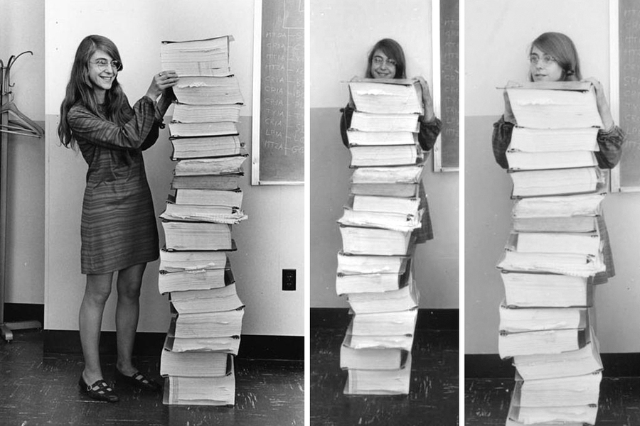
Welcome back everyone. In this video we’re gonna be talking about software engineering. Now you should remember this particular machine the ENIAC, which was the first electronic computer in the United States. Programming the ENIAC was a really slow and laborious process though. To load a program, ENIAC’s programmers Pictured here is Gloria Ruth Gordon, and, well, later Bolotsky, and Esther Gordon would physically rewire the hardware and a new configuration corresponding to the calculations indicated by the programmers. And so you can see them here moving actually the wires from different plug boards for the computer to actually make different calculations and operations work. So the task was made even more difficult by the secrecy involved with the machine. Initially, programmers weren’t even able to see the schematics of the machine and had to pass their wiring instructions belong to the technicians. So the programmers didn’t weren’t even instructed on how the actual machine was built or how it worked. And they couldn’t even actually run their program themselves. So you could imagine that that would be a really difficult task to actually accomplish writing successful programs for a computer that you didn’t even know how it worked.
But this was very similar to Alan Turing’s original conception of the his famous Turing machine. And this machine had carried out hardwired instructions on data encoded as zeros and ones on an infinitely long paper tape. Turing had an epiphany with this machine, realizing that by making this machine read instructions on specific sequences of zeros and ones, as his machine booted, he could encode the program directly on the infinite tape with the data it was actually operating on. Now, this is a huge leap, because before right with this, we had a tyranny of numbers problem where the We’re just getting so complex, that it became nearly impossible to make anything substantial in today’s terms of software.
But now that we can actually store the actual software alongside with the data actually being used the started to simplify the process. These ideas were incorporated into electronic computers by several computer scientists, including J. Presper Eckert and John Mauchly, inventors of the ENIAC computer, as well as John Von Neumann, who was the first to publish such an article about this architecture in this paper, the first draft of a report on The Ed vac. For this reason, a computer architecture allowing for stored programs is referred to as the Von Neumann architecture, and is the basis for modern digital computers. Stored programs also allowed us to develop bootstrap code or libraries of common procedures that can be reused for future programs. And we’re loaded into the computer as it was warmed up. This is an important predecessor to modern programming libraries and operating systems. So as you can imagine a lot of these early computers, you ended up having to actually program basic operations anytime you actually wanted to work with something. So a lot of the software, a lot of things were done by hand, a lot of the things that we take for granted like user input, a lot of the mathematical operations that we use in modern programming languages, all of these libraries that we utilize to make our software a lot easier to write, and which allows them to be extremely functional and easy to read. And these weren’t existing or at least didn’t exist in a lot of the earlier software that was actually being developed. So our ability to store programs along with data and store programs, along with the actual system itself. Made a lot to future programs a lot easier and faster to write.
But the next major invention in software design was the development of programming languages and the associated technologies of compilers and interpreters that allowed programmers to write programs and a higher level programming language that would then later be translated into machine language for a stored program computer. Pictured here is Grace Hopper, the creator of the first higher order programming language flow Matic and influential co creator of COBOL. A very popular or was very popular business programming language. The development of programming languages is especially important in that it allowed us to develop abstractions for simplifying development of software and allowing us to express significantly more complex ideas in computer code without a significant amount of more lines of information and code that had to be made with the software.
But as programming languages diverse From their mathematical roots, and became more expressive, new challenges arose in making sure that programs were clear and easy to understand. This is further complicated by increasingly sophisticated nature of software that sought to accomplish more than earlier programs had ever had. Furthermore, the growing industry demand for software developers had led to often incompletely trained programmers entering the field. And so if you could even code a little bit, you probably could land a programming job. This is a pretty important turning point in the industry here because we had a rapid growth of actual technology. So not too long after world war two ended, electronic computers started to become smaller and more popular and they all of a sudden didn’t take entire rooms to actually build right they weren’t the size of school buses anymore, especially as we approached the personal computer era.
We needed a lot more people to actually program there was a significantly higher demand for software and the demand for that software was even greater yet as far as the functionality would actually go for that particular software. So, as a result of all this sloppy programming, poorly understood designs and really the lack of systematic planning and execution, with these poorly trained programmers led to an era of our field being labeled as the software crisis. This spurred the development of a lot of different new technologies and approaches and approaches for developing software.
Some of the key projects from this period include the IBM O’s 360 project that ran drastically over budget while employing over 1000 programmers, and famously the fair act 25 radiation machines which would regularly display an error to their operators. So as a nurse would come in, and try to to administer a dose of radiation to let’s say, a cancer patient, they would then try redoing the treatment because there was an error on the machine on on the screen or whatever. And they wouldn’t realize that the machine had already delivered a dose of radiation, which led to a lot of patients actually dying or being crippled.
Throughout the software crisis, a lot of important computer scientists made a lot of developments in contributions to software engineering, and one of the more important computer scientists of the day, like Edgar Dykstra and Nicolas Wirth sought to address these challenges through language design and better education for fledging budgeting computer scientists. This 1968 letter to the editor of the ACM journal by Dykstra underscores his concerns with the goto statement, which allowed for a very disjointed style of programming that would make programs difficult to debug and understand as the go to statement would allow you to jump back and forth between steps in your program without any concern for anything else. This and readability of and usability concerns as well as efficiency issues became one of the driving forces behind the evolution of programming languages. Where most currently use programming languages don’t even have a go to statement like Python, and many of the many of the other popular languages that we use today. Other improvements included the addition of modules and information hiding, introduced by David Parnas concepts that eventually involve evolved into what we refer to now as the object oriented programming languages.
In the same year, Margaret Hamilton, one of the NASA engineers responsible for simulating the Apollo missions on a computer. One of the most involved computer simulations attempted to that time, coined the term software engineering to describe the role she had played The stack of documents Next to her is actually one of the simulation results from that effort, which helps underscore just how large software projects were growing at that time.
Now that we’ve talked a bit a little bit about the history of software development and software engineering and how it’s evolved over the years, what are some of the key activities that we actually engage with in this process. Now, you’ve already used and worked with a lot of these already, even if you haven’t really made the connection to them yet. Software Engineering overall will come with quite a few different processes along with it. But overall, you can kind of expect these six different stages.
Now, to begin the process off, we’re going to start with requirements gathering are going to actually go around and collect information about the software that we’re actually being tasked with to develop. So this involves with going and meeting with clients meeting with users meeting with business folks meeting with just about Anybody and everybody that might be a stakeholder or involved with actually using that software or funding that particular kind of project.
Now, once we have gathered all of the requirements for the software, then we can make the jump into the software design. So here we’re going to start to architect the project and lay it out overall, but we haven’t actually even done any programming yet. That doesn’t actually typically happen until the design has been actually completed. So once we actually start the implementation, then after the code has been finished, or at least a stage of the code has been finished, that code is then split off into the testing phase. Sometimes the implementation and testing phase, you might see done as one as if you’re on a small team or depending on the kind of approach you’re actually taking to the development lifecycle.
But after the software has been fully tested, then it gets deployed or installed. And then it goes into like a maintenance mode, right. So a lot of times you get the first Windows updates and various other software updates on mobile apps and games and everything in between. So that’s the maintenance phase, right, where we’re trying to update patch, fix anything that may actually been broken, or things that we didn’t catch during the testing phase. But you see that now I’m back at the requirements gathering.
Most of the software development life cycles that we actually see an encounter are a never ending cycle. Software is never perfect the first time around that we actually build it. So more often than not after creating what we refer to as a prototype. We’re going to end up going back to the requirements gathering stage, talk to our customers, talk to our consumers, talk to our stakeholders, and give another shot at it. Whether or not whether it’s just a, a simple update, or feature addition, or even a complete rewrite in some cases if we didn’t get it right the first time. But let’s take a look at some of the early software development life cycles that were developed. Now, you’ll notice that these each of the activities that we just talked about before lend themselves very well to a systematic step by step approach, where each activity is followed by the next and we kind of loop back onto this.
This is essentially the approach that was developed as a standard strategy for software engineering after the work by Margaret Hamilton in the early 1960s. And over the next few decades, an approach that we call the waterfall model of software development for reasons obvious from the graphic, where each phase flows from the next into a highly linear fashion now In the waterfall development, as I mentioned, right, this is a very linear process. This isn’t like the software development lifecycle that we’ve showcased earlier, where we start with the requirements gathering. And we cycle through each phase. And we end back up at the beginning of the waterfall method assumes that each phase is done in one shot, so there’s no reduce.
So we gather the requirements and design the software, implement it, test it, so verification, and then we go into the maintenance mode. So of course, we install and deploy the software in between there. But once we’ve deployed the software and enter maintenance mode, we’re not going to actually be going back and doing more requirements gathering or redesigning anything, it’s just some simple bug fixes at that point. So, it emphasizes the waterfall model emphasizes that the actions are arranged as discrete phases in sequential order, although depending on the model that you actually look at some splashback is acceptable. So if you imagine an actual waterfall, some water gets splashed back up and falls back down. So maybe we get to the implementation phase, but we recognize that our design is severely flawed. So we may bump back up, change the design a little bit, and go back down into the actual coding phase.
But here, the entire system, and the waterfall model is implemented, designed and deployed all at once. So planning, scheduling, target dates, budgets, all of those things are set in advance. Most of the time, these are often set by contracts. So there’s really no flexibility there with as far as funding and deployment dates go. A lot of times with the waterfall model, there’s a lot of extensive documentation and very tight control. So this is a very heavily managed process. So this is really useful for processes that require a little A lot of structure. And we’ll talk about some other models here in a little bit that have a lot less structure, and that offer a much more flexible approach to software design.
Additionally, during this time, scientific management techniques were adapted for use in the management of software developments. One of the landmark books capturing this evolution was Barry Boehm’s Software Engineering Economics book, where he argued for considering trade offs between adapting existing software and creating new software on economic terms. And so we use statistical analyses to develop equations like this one, seeking to equate development time in main years to the metric of software lines of code, or SLOC. Now, there are there’s a lot of debate around measuring the productivity of let’s say, developers and cost of software based off of the number of lines of code that are actually produced. And there’s a lot of fallacies behind that metric as well. But a lot some people actually some fall into that trap.
Another book from that particular time period refutes some of those both some of those arguments as I mentioned, they were very controversial. But this book, the mythical man month, details many software engineering management fallacies. Like, for example, adding more programmers to a late project will absolutely right help it finish sooner, but not so much. In practice, bringing new developers up to speed consumes much of the current team’s time, and overall slows the development. So let’s say you’ve been working on this really big important project for nine months. But you are a couple, maybe a month or two behind schedule. So management comes in brings in new developers to try to help get you back on track. But it actually ends up putting you back farther in your time schedule because you had to stop your productivity to get the new people caught back up to speed.
Another fallacy here that is discussed in the mythical man month is the use of crunch time. Crunch Time is typically portrayed as an increase in productivity, right. So, you know, spending, you know, 60 to 80 hours a week to meet that deadline. So, pulling 18-20 hour days, programming all night, I’m sure you have probably done this when studying for a really big exam. Crunch Time doesn’t necessarily increase productivity. Studies have actually shown that a breakeven point for let’s say software development lies around about 35 hours. There’s been research that shows about 30 a year your average limit for a software developer is about 30. 35 hours of programming per week. Beyond that, a fatigue programmers introduce more bugs into their code at a faster rate than they’re actually removed. So that ends up costing a lot more money and time because they’re, you know, fatigued. Developers that have just been coding for too long or going to be more prone to produce bad code. I’m sure some of you some some of us have experienced this as a student, as I mentioned, as you’re studying, you know, when you’re really exhausted, or have had way too much caffeine are way too much coffee. You may not be studying as efficiently or or productive. Your productivity may not increase proportionally to the amount of time that you’re you’re actually spending versus the amount of time you’re spending when you weren’t exhausted.
Let’s take a look into a few other different methodologies in software development. So this one is in complete contrast to the waterfall model of software development and pretty much all other development methodologies. Because this methodology, there really isn’t anything to it. It’s generally known as cowboy coding or code and fix. Now, this in many ways, is the anti software engineering approach, where planning, testing documentation at pretty much everything, all of that is ignored, or immediately writing code. And predictably, this leads to a lot of what we refer to as spaghetti code. And so it’s just mangled structure that has really no clear way to it at sprinkled with sub optimal algorithms memory leaks, structural issues is just a mess, right? Imagine getting out a box of Christmas lights that were just thrown into a box and in January, and you go back in December, try to put those Christmas lights up. And magically, they’ve aimed together into this big ball that takes hours upon hours to actually unravel. And sometimes it’s just easier to throw it away and start from scratch.
Even more unfortunately, with this methodology of cowboy coding, this is actually unfortunately very much how most students learn to approach software development and their early assignments. And it’s often carried with them into industry. So the sooner that we can actually start to teach design structure and this process, the better habits that you will develop, especially as you start getting closer to working to working to an internship and into To a full time job.
But not surprisingly, issues in software engineering are typically coupled with periods of surging growth for a field of computer science. And so this graph here based off of data collected by a tabulate survey tracks the growth of Bachelor’s of Computer Science degrees since 1966, up through about 2010. Now, you’ll notice the two very clear spikes in this graph, one peaking around 1985 and the second around 2004. That first rise was a big issue here for K state and many other universities that that matter, to and to meet the growing demand of students with the limited faculty available to graduate students taught and many of the undergraduate courses, similar measures were employed at other institutions likely compromising the quality of preparation for an entire generation of software engineers because people were thrown into teaching positions that really weren’t that well qualified to teach those particular topics are experienced enough.
A similar trend occurred during the second peak, although thankfully not so much with us. But hopefully you can maybe guess what the driving force was behind that growth rates at that time, right. So this peaked around 2004. That was around the.com. Boom. So the first search that we saw began in the early 1980s when the personal computer started to be introduced. And so that spikes the first surge and the demand for computer science degrees, and then the second peak reflects the dot com bubble. So as the internet came out in 1990, we saw a huge burst in the late 90s of companies thinking, Ah, well, we can make it big if we get on the internet. Okay, and so we saw a huge surge In the need for computer science. But after the.com bubble burst, which burst in the early 2000s, we saw a rapid decline in the demand for computer science degrees. But thankfully, over the past few years, we’ve since then we have seen a increase, and the demand for computer science or an increase in the number of degrees awarded in computer science. And we haven’t seen that die off quite yet.
But with the growth of the internet, Internet companies and the eventual collapse and the success of all the survivors to underscore the need for a more reactive and flexible style of software development that was possible with the waterfall model. So the dot com boom, sparked a lot of different kinds of needs of technology and software, especially with the invention of the internet, of which we had never actually developed software for something like that before. So the web needed to be what robust, secure and most importantly, scalable. And so that meant cowboy coding couldn’t meet that need either, even though it was super flexible, because we could just start with no planning whatsoever. But that often led to very insecure software and software that really didn’t scale well. So new strategies as a result of the dot com boom, emerged to create more robust software engineering approaches, and these were started to be employed more widely.
One of these of course, was just simply prototyping which is especially useful for developing experimental or difficult to estimate systems. And so the idea here right is to build a prototype, establish the base functionality, complexity and worth wildness of the of the specific product right. So this begins with implementation or coding and then leads to other activities, like requirements gathering and software design. So try something out and see if it works. See If the Customer likes it. If they liked Or let’s say they like this, but not that let’s keep things that they like and throw away the stuff they don’t want. So this is pretty much the cowboy coding or the code and fixed process with a more developed and structured approach, right. It’s not just a standalone process. There’s a lot more involved and there’s a lot more structure here.
The iterative development process, or the iterative development model breaks down software development into much smaller segments. This allows for a lot more change and variation to the development cycle. So the iterative development process works by working through many waterfalls. And so if you look at each one of these chunks here, each one of these stages, they’re pretty much the waterfall process. And so overall requirements are gathered, then we analyze those requirements develop, implement test, and this is a cycle right? In this case, our waterfall is circular so we can keep on trying Go Go, go, go go. And then we’re going to release a prototype or a version of our product. As we go through this each time a release, we demonstrate that to our customer. And get feedback and then we’ll work that back into our next cycle. And so we just keep on iterating this until we are doing our final release to our customer.
One more different developments that we want to talk about this time is actually proposed by Boehm, this combines prototyping and the waterfall development is very similar idea to iterative design. The spiral development model focuses on risk assessment and management by breaking projects into smaller parts, allowing for the evaluation and change as each part is individually finished. And so this works off of four main segments. So you are going to determine the objectives, alternatives and constraints of that particular iteration. So that small part, evaluate alternatives, identify and resolve those risks. So we want to try to match negates the risks because those risks, right, the more risk, the more cost is actually involved with the project. And then you’re going to develop and plan for the next iteration. So as you start to cycle out here, right, so you’re starting small, the center here, you’re going to start with very small projects, right. And as you complete those smaller projects, the base of the foundation of your software that’s going to slowly grow out, and you’re slowly going to introduce more things that are needed in the project, like different models, different prototypes, more testing, and the closer you get to the outside edge of the spiral, the closer you’re going to get to deployment. But this is again, right like iterative design, much more flexible, and overall, much more appropriate to what modern software actually lends itself to.
But even more so after this We actually come into something that’s very popular industry today called the Agile process. These methodologies that we’ve talked about so far were to being developed by software engineers and high level planning positions. A new philosophy was emerging from the rank and file developers which, as expressed in this Agile Manifesto, the manifesto reads as we are uncovering better ways of developing software, by doing it and helping others to do it. Through this work, we have come to value individuals and interactions over processes and tools, working software over comprehensive documentation, customer collaboration over contract negotiation, and responding to change over following a plan. That is, while there is value in the items on the right, we value the items on the left more. So while agile is often thought of as, as a software engineering process By itself, it’s not. Rather it’s a guiding philosophy that can be applied in conjunction with many other software development approaches. That said, it clearly works better with something like iterative or spiral development or any other reactive styles of software engineering than the more rigid approaches that embodied the waterfall approach. And so as part of the reading, I’m going to actually ask that you go check out the Agile manifesto.org website and honor they have all the principles that are assessed with agile development and kind of embody what agile actually means.
But overall in the Agile process, you’ll typically see something like this agile as it stands right is the philosophy behind it as extreme flexibility. In this sense, you work off of mostly what we refer to as sprints. So these small Sprint’s will always have some sort of deliverable. product to the consumer or the customer. So it’s looks very similar to what we see with the software development lifecycle and a lot of the iterative or spiral processes where you brainstorm or gather requirements, you design prototype, develop, you QA. So you test and test and test and test. And then you deploy. And as you deploy, you do a little bit more testing, and you deliver that product to your customer. Or maybe you deliver that to the next person up in your organization. And all that feedback is then worked back into the next iteration into your next sprint. And so typically, what you’ll see with Agile process of the Agile process or Agile software development is that each sprint will focus on one or two small features of the software. And once that feature is actually completed, then the that particular developer will move on To the next sprint with the next development of either that same feature with modifications that were given to them by the consumer, or moving on to after completing that feature moving on to the next.
Another improvement that came in the mid 90s was the development of a suite of standardized diagrams for modeling software. The Unified Modeling Language, or UML. UML allowed for complex software systems to be diagram discussed and shared between developers and an easier to interpret form. Because before then there was no standard for documentation or not necessarily, but there was a lot of complex software being developed and each programmer would document and diagram in their own unique way. Just like what we would have, we have our own unique way of speaking and writing. Each developer had their own way. of not only just writing their own code, but also diagramming and and discussing about that code. And so UML offer a standardized way to actually share the overall structure interactions. Things like the activity or sequence or flow of the program among different developers, actually was someone who’s actually been trained with you to interpret and read UML could understand the software at a much higher level, a much deeper level, even without knowing how to actually program. But for now, this is going to conclude our discussion on software engineering, software development. There’s obviously a lot more here that we did not cover. In future classes we’ll take a much deeper dive into the architecture, modeling and development of software.
Read Pattern on the Stone, Chapter 8.

In this module, we’ll discuss the field of human computer interaction or HCI, sometimes referred to as computer human interaction, or CHI. It is the study of how computers and humans interact and how we design computers to better support humans in that efforts. HCI is one of the fields that we’re going to look at it throughout the semester, we’ll do this several times.
The field of HCI has a few goals that are very important for us to keep in mind. First and foremost, HCI aims to try and make the world a better place through the use of easily accessible technology. It allows us to work to understand data that is being presented to us, and it helps people interact and communicate with one another using modern technology. But Finally, and most importantly, the major goal of HCI is to give people better control over the tools, computers or machines that we’re using in our daily lives.
So how do we do this? Important part of the field of HCI is studying and designing and applying all the things we learn about interactions between people in computers. Sometimes we study how people interact with computers. And sometimes we have to study how people interact with other people, and how we can bring those ideas to the computer. And so to do this, we end up using results from a lot of different fields, not just computer science, but the fields of cognitive and behavioral psychology, design, Media Studies, graphics, art, music, all of these things can go into the field of human computer interaction.
One of the pioneers of the field of HCI is Douglas Engelbart. In 1950, Douglas Engelbart had graduated college, but really had no idea what he wanted to do with his life. And so he set out to try and determine how he could have a greater impact in the world and came up with this really interesting idea that we’ll look at in just a second. But his ideas really lead to the field of human computer interaction as we know it today. And he’s responsible for it. Large part of how we use computers, I think you’ll find it really interesting to see the things that he came up with during his time. So as we talked about Douglas Engelbart was a student in the 1950s, and was really struggling to figure out what he wanted to do with his life. And so eventually he came up with this idea for a motivation to help him work in computer interaction. So first and foremost, Douglas Engelbart decided that he wanted to make the world a better place. That’s all well and good, but you really have to understand how to make that happen. And he realized that to make the world a better place, it required a large amount of organized effort. It wasn’t anything that one person could do on their own. So how do we get that organized effort, but we have to bring together the collective intellect of all the people in the world working to solve these really big problems. That is really the key. And so Douglas Engelbart realized if that process was somehow made easier, he could effectively boost the work of every person working on all of these large Scale world problems. And that is what led Douglas Engelbart to the field of computer science and HCI. He realized that if he could make modern computers more effective, more efficient and easier to use, that that would, in effect, boost the effort or everyone working on these problems, because it would allow them to come together and harness their collective intellect to put forth organized effort to make the world a better place. So as we said, computers are really the key here and that’s what Douglas Engelbart realized.
One of the greatest creations of Douglas Engelbart work is the computer mouse shown here. It’s the first example of a interaction device built specifically for a computer that really revolutionized how we interact with computers. He developed the computer mouse in 1967, while he was working on the design of a computer system called the online system or in Is that we’ll look at in just a second. And he originally patented it as an X Y position indicator for a display system in a video that will take Look at he actually jokes a bit about why it’s actually called a mouse today.
But as we said the mouse is just a small part of what Douglas Engelbart was working on. His true work revolved around the online system or in NLS computer system that he developed. The NLS was really the world’s first modern operating system to include features such as a mouse hypertext links that you could click on a raster scan video monitor that actually gave live feedback to the user, the ability to do screen windowing, where you could have multiple things on the screen at the same time, he was able to use that system to build presentation programs that are very similar to what we do with PowerPoint today. It allowed him to organize information in radically new ways that had never been seen before on a computer system. And it even allowed for collaborative editing and messaging, very similar to the tools that we use today on the internet.
And the amazing thing about this system was it was demonstrated in 1968 in what has been called the mother of all demos. Douglas Engelbart demonstrated all of the features of the online system during a single live demonstration in December of 1968. He assembled over 1000 computer professionals in an auditorium. And with double Douglas Engelbart sitting at the front at a computer console. He seamlessly demonstrated the power of his NLS system, showing new idea after new idea to these people. And he left his audience completely spellbound. And to this day, it still stands as one of the most important and most unique computer demos of all time. Oh, and by the way, he was actually using it to control a computer that was over 30 miles away. So it was done remotely. And to put this in context, remember that December 1968, is several months before we landed on the moon in July of 1969. So even though we were sending people to the moon, we’re in spacecraft that had less power than a graphing calculator. Douglas Engelbart was setting the stage for a computer lead to revolution in how people use computers today.
The best part about the mother of all demos is that a recording of it exists so that we can watch the whole thing even today. As we mentioned, he combined some real cool state of the art technology in this single demo. He used live video projection, he used teleconferencing and video conferencing. And for a lot of people in the audience, it was the first time they had even seen a live computer display something that we take for granted today. So on the next page, we’re going to take a look at a few short clips out of this mother of all demos, and we’ll have some short discussions about what exactly he’s showing on these clips.
The full video of the Mother of All Demos is linked below, but it is nearly 2 hours long. While we’d love to have you watch the whole thing (and you are more than welcome to do so), we wanted to highlight a few of the more important parts. Listed below are the timestamps for a few important sections and a bit of discussion about each one. Feel free to skip around to watch a few of these sections to better understand what Douglas Engelbart was presenting.
On the previous page in NLS was a very revolutionary system. Unfortunately, it was very hard for the average user to use. And so it really never could gain that mainstream reputation that it wanted. So we had to come up with an easier way to use modern computer systems.
And as the story goes, and engineer one day was staring at the top of his desk thinking about how to solve this problem, and that solution came to be known as the desktop metaphor. What if we build a computer system that looks and acts and feels like the things that we’re used to in the real world, we can have a desktop with different things open on it as we’re working. We can have files and folders full of files that allow us to organize information, and we can move things around quickly and easily to get us different views of the same thing.
This is what most modern computer systems were built around, and it was first introduced all the way back in 1970. This picture shown here is from the Xerox star workstation in 1981, which was one of the first real mainstream computers to use the desktop metaphor. Of course, in those days, one of the things that computer companies were really well known for is borrowing or stealing other ideas from other companies. And so Apple stole basically the same desktop metaphor idea for its Macintosh desktop from 1984.
And there’s always been a little bit of discussion about who actually came up with it first, this was actually dramatized in a TV series called The Pirates of Silicon Valley. So let’s take a look at a short clip from that TV show to give you an idea of what things were kind of like at that time.
So now that we’ve seen some examples of historical computer interactions, let’s talk about what it might take to make a good computer interface today. Think about the computer systems that you interact with on a daily basis. What about them makes them easy to use or difficult to use? Would your answer change if you gave that computer system to a toddler, or maybe your grandmother or an elderly person? So really good human computer interaction or good computer interfaces can depend widely based on the needs of the audience. Of course, there are some things that we can think about that make good human computer interactions. For example, we want it to be functional, it needs to do what it says it does. It needs to be reliable, it should always work the way we expect it to. It needs to have a high level of usability. So it’s something we can easily and effectively work with. It should be efficient. We don’t want to have to click 18 times to open up a single web page do we? It also should be maintainable both from the ideas of the user, it should be easy for them to keep their computer up and running. But it should also be maintainable on the software side for the developers that are building these apps. And one of the things that I think is often overlooked in the field of HCI, is it should be portable. We really want the same ideas to work across multiple different devices and even multiple different paradigms. And that’s something we’ll talk about a little bit later.
To really develop good HCI we have to follow this iterative design process where we start with an existing device, we analyze that device, we check our requirements, and then we can slowly make things better. It’s really interesting to think how computer systems have developed over time. And there’s some great YouTube videos looking at this, for example, considered the original iPhone design versus what we have in our modern iOS, or consider some of the earlier versions of Windows compared to the modern versions we use today. While those systems are very similar, we can see that there’s been a slow iterative design process that has slowly improved the design over time, based on the changing hardware and our changing understanding of good HCI.
Of course, good HCI also relates to a lot of different fields. We have to think about things like psychology, such as the fields of memory and perception. How do we remember things? How do we perceive things on our computer? We have to talk about sociology and how interacting with computer changes how we interact with other humans. We look at things like cognitive science, we look at ergonomics, how easy it is for us to use a computer system, we can think of things such as graphic design and interaction design, what colors and shapes and buttons would tell us. We can even think of things like speech language pathology, should our computer refer to itself in the first person or the third person? How should it interact with us? And we can even think of really interesting fields such as phenomenology, the study of consciousness, how do we make things on our computer such as that we are consciously aware of What our computer is trying to tell us. And we’re not just ignoring it and clicking next all the time.
So one interesting case study from the field of human computer interaction is the case study of automated adaptive instruction. Automated adaptive instruction is the idea of providing the user with instructions based on what the user has done previously, and what we think are some possible next actions of the user. We’re all familiar with our phones autocorrect system, how it can predict the next words we’re trying to enter. Gmail recently has done this as well. That’s kind of the same idea. But instead of just filling in words, it’s actually telling us how to use the computer system and how to do what we want to do next. This really came about in the 1990s as users were getting used to the personal computer, but they were becoming overwhelmed by the complexity of the technology. And companies such as Microsoft turn this into a very lucrative area of research.
And so probably the most interesting case study from adaptive instruction is the computer program known as Microsoft Bob, hopefully you’ve heard of Bob, but if not, this will be a really interesting thing to talk about. And I get really excited talking about this because when I was young, the first computer my parents bought came with Bob pre installed. And so my first computer interaction was actually with Microsoft Bob. This is what Microsoft Bob looks like. The whole idea behind Microsoft Bob was to take the desktop metaphor to the next level. And instead of having a desktop for our computer, we could mirror an entire house. And so our house would have a whole lot of different rooms, we could have the living room, where in this room we have things such as a Rolodex that represent our address book, we have a money bag that represents our finances. There’s a checkbook sitting on the table that represents our Quicken or our check our money software. And that was really the idea you would have things in your house in Microsoft Bob, that mirrors the things that you would use in the real world. And by clicking on those objects, you would opened the programs that related to that. And then of course, you could have different rooms, you could have a living room with all of this, you could have an office with different things, you could have a kid’s room with all the games in it. And so it was a really neat idea.
But of course, the automated adaptive instruction part is the little dog that we see here. This dog is called rover, and rover was there to try and help you navigate Microsoft Bob, it would offer to do things like help you find a program, go to another room, add something changed something, anything you wanted to do, you could interact with rover and rover would help you figure out how to do it. And it was this really neat idea. Unfortunately, I think Microsoft Bob really wasn’t quite ready for primetime. And graphically, it doesn’t look very good. And in fact, most computer users had gotten used to the desktop metaphor. And so the power users weren’t exactly excited about it either. And of course the biggest nail in the coffin was Bob itself wasn’t that great of a piece of software in some ways. It was kind of buggy and did crash a lot. How There are some people that really are big fans of Microsoft Bob even today. And so if you look online, there’s some great videos of people who have installed Bob even on a modern computer just to see how it works.
Of course, this did lead to some ideas that stuck around. For example, rover became the search assistant from Windows XP. And of course, this is the source of the infamous Clippy office assistant from Microsoft Office 97. Again, it was the same idea. Microsoft Office has a lot of features that most users don’t know how to do, such as mail merge. And Clippy, even though Clippy might have been a little bit annoying, was perfectly capable of helping you figure out how to do that. And so it kind of got a bad name, but it did have some neat ideas.
The big lesson learned from these assistive agents is companies were trying to teach users how to use computers, instead of trying to design computer systems that work the way users expect them to. And so in a lot of modern computer design, instead Have all of this instructive bits, you see us trying to more and more build computer systems that act like we expect them to. A great example of that is on your phone. If you scroll up at the top of a web page, it tries to refresh the webpage. This is especially notable on social media sites like Twitter or Facebook, you’re scrolling up looking for new content. And so it immediately reacts to that and does what it expects you to think it wants to do.
So of course, there are a lot of virtual assistants out there today we have Clippy. In 2011, we had the release of Siri on Apple devices. We’ve had Google and Cortana. And now we have other devices such as Alexa. And so we’re really into the smart, the age of the smart assistant where almost every home has a smart assistant in it. Almost every device has the capability of using one. And so we’re really seeing this come into its prime today. So what were the big lessons learned? Well, of course, this led to a lot of different ideas, such as searches on Google, if you’ve ever searched for something on Google, and you get that Searching? Are you sure you didn’t mean X? That’s an example of adaptive instruction. It’s telling you how to do things on Google.
We also see context clues on our touch interfaces, where if we swipe left and right, when there’s nothing there, it will still let you swipe and show you that there’s nothing over there to be able to swipe to. And so like we talked about earlier, the big legacy here is, instead of trying to change human behavior, we want to try and change the program to fit the expected behavior of the human. Or to put it more concisely put things where people expect them to be.
One person who’s very active in the field of HCI today is Don Norman. Don Norman was a 2006 Franklin medalist. And he’s really famous for writing a book called The Design of Everyday Things, which if you haven’t taken a look at it, I encourage you to at least look at the front cover of that book and see what he’s talking about. Don Norman is a real big proponent of designing things to be how they’re expected to be used instead of design just to be interesting. And he talks about some really great examples of designing for everyday things. And so after this video, we’ll take a look at a short clip of Don Norman talking about some of his work, and hopefully, you’ll start to see the things that he saw in the real world that helped us understand modern design.
So one of the important things to remember in HCI is that iterative design process and designs change over time. For example, on this slide, the top picture is a picture of Microsoft Word from version two 2003. And the bottom picture is from a much more modern version of word that we use today. In 2003, the version at the top was very well regarded, it had a toolbar with lots of easy to follow buttons. And a lot of people got used to it and really liked it. And so in 2007, when they switched from the toolbar design to the ribbon design that we use today, there were a lot of users that really didn’t like that design. And if you get down to it, it really turns out that those users didn’t like the design, not because it wasn’t a better design. They didn’t like it because it was different. And so one of the things we’ve struggled with in the field of computer science is design changes for change sake is not good, because a lot of users don’t like change. But if we change things for the better, eventually users will get used to it. And thankfully, we’ve seen over time that users have very much gotten used to the new ribbon style and they do understand that it is much more efficient and much easier to use than the old toolbar style, but there’s always still little bit of fear of change that always comes into this.
Another good example of this is Windows, we’ve gone from Windows XP to Windows 7 to Windows 8 to Windows 10. And each time we’ve changed a little bits of how the Windows computer system works from different toolbar designs, two different Start Menu designs, two different designs for things such as the control panel and touch interfaces. And each one of those designs might be based on a lot of really good research, but it’s changed and a lot of users are very resistant to change at first. But of course, some changes are really good. For example, in Windows XP, if you had a blue screen, you would get something that looks like this. This error message isn’t really all that helpful is it? It’s got a lot of technical details. But for most normal users, it just scares them and they don’t really know what to understand. And so a more modern computer system has a little bit friendlier, have an error message that tells you what’s happening and it tells you what’s going on but it doesn’t just bombard you with more data than you actually need.
So what is the future of HCI look like? It’s really hard to tell, but there are tons of things going on. After this video, we’ll post several videos for different views of HCI. And some of the things that have been out there in research or in industry today, for example, different user interface concepts such as 10 GUI, different ideas around ubiquitous computing, such as the Google Glass project from a few years ago. We can look at 3d tools today, such as the Oculus Rift, and some of the new 3d virtual reality tools. And we can even talk about accessibility and how we can design computer systems that use just a single finger to allow you to type text very, very fast with a minimal amount of inputs. And so I hope by looking at some of these videos, you’ll be inspired by the different ways that computer systems can be interacted with beyond just the keyboard and mouse that we’re used to today, and it will encourage you to think about different ways that we can build computer systems in the future.
Read Pattern on the Stone, Chapter 9.
A fundamental part of today’s world! Let’s learn how it works, and how we can write webpages ourselves!

In this module, we’re going to talk about the history of the Internet. The history of the internet is a very interesting topic in computer science. But I think it’s one that we don’t think about very often today, we just take the internet for granted and just know that it’s always there. So let’s take a look at where the internet came from. The internet was really built to solve a unique problem.
Networking is complicated. And in the early days of computer networking, the only way two computers could talk to each other was via a direct connection between those systems, much like the phone systems of the olden days. And so we’ve already seen some network connected computers such as the NLS system that Douglas Engelbart talked about, for example. But networking was really complicated. And so because of this, we had to have direct connections. And it was very slow and very tedious to have really powerful computer networks. We ran into problems that were very similar to the tyranny of numbers problem that we talked about in an earlier Module. So the internet was really created to solve that particular problem.
One of the visionaries of the creation of the internet was J.C.R. Licklider. Licklider was a computer scientist at the defense, the Department of Defense Advanced Research Projects Agency, or DARPA. And he was interested in how we could build computer systems to aid the work of his agency. And so his work was really around some of the earliest networked computers such as ones at MIT in Santa Monica. But the real frustration he had was each one of those computer systems required a different terminal and different commands to interact with it. And J.C.R. Licklider really dreamed of having just one computer terminal on his desk, and one set of commands that he had to memorize. And from that terminal, he could access any computer system nationwide to get the information that he needed. And so he really famously talked about this and came up with some really interesting ideas. Let’s take a look at a video of J.C.R. Licklider talking about his ideas For what became the internet.
Man-Computer Symbiosis by J. C. R. Licklider
J. C. R. Licklider his idea inspired him to write a paper in 1962 titled Man Computer Symbiosis. And in that paper, he had this quote, that he foresaw a network of such computers connected to one another by wideband communication lines, which could provide the functions of present day libraries together with anticipated advances in information storage and retrieval, and other symbiotic functions. And while there’s a lot of words here, he’s really thinking about building computer connections where computers can store libraries worth of information that we can access at our fingertips.
And so a few years later, he started talking with his colleagues. And he came up with this idea of what he called the intergalactic computer network, which I really admit I wish we called the internet the intergalactic computer network, I think is a really catchy idea. But he envisioned this idea of a global network of computers all interconnected and accessible to each other. And so you can easily ask access data from data and programs from any of those computers on any other computer. And he actually even submitted a memorandum called a memorandum for members and affiliates of the intergalactic computer network to encourage people to participate in this new idea. And while this never really came to be, this idea of forms the basis of a lot of the internet and cloud computing resources that we use today in our daily lives.
Another major figure in the history of the internet is Leonard Kleinrock. Leonard Kleinrock was a major figure in the history of the internet and was a researcher at UCLA. And he helped develop the technology behind packet switched networking, which we will take a look at in the next lecture. And it was really developed and proposed to the government as a way to build computer systems that were very fault tolerant in case of an attack or an emergency. His work was really revolutionary. And there’s actually a great video of Leonard Kleinrock himself discussing the importance of his work at UCLA in the early days of these computer networks. So let’s take a look at that video.
On October 29, 1969, the first message was transmitted across the newly created ARPANET between computers at UCLA and SRI, the Stanford Research Institute. And so in this particular picture, we see the notes from Leonard Kleinrock notebook taken on October 29, 1969, showing that they talked to SRI hosts to host and it was really revolutionary moment on the internet. Because this was the first instance of a packet switch network being used that now forms the basis of the internet. Of course, it wasn’t exactly a success. They tried to transmit the word login, but only got the letters L o before the system crashed. So it wasn’t exactly a huge success, but it was a very small step toward the creation of the internet.
And so with that, ARPANET was born, ARPANET was the Advanced Research Projects Agency Network, and it was really the first computer network of its kind in the United States. Connecting all sorts of research areas together. Above me is a picture of the ARPANET map from March 1977, showing several hosts all connected to the network and all the different ways that they talk to each other. It was originally started as a packet switch network of just four different sites that were connected to these devices called interface message processors, or IPS, which are really modern, early precursors to what a modern router does, taking the messages from a computer and translating it so that it can be sent over a packet switch network.
Of course, ARPANET wasn’t the only network at that time. As we saw in the video at the beginning of this module, there are many different networks created all across the world. For example, with ARPANET by the 1970s, there were sometimes 20 new hosts coming online every day, you had the National Physical Laboratory in Great Britain, you had merits, the Michigan Educational Research Information Triad. You had supply days in France, and then you had the proliferation of public networks such as X25, and Usenet. Which were all public networks that were available through telephone providers at that time.
But all these different networks were disconnected you really couldn’t get from one network to the other network. And so we needed something else to really build the modern internet that we use today. And so that comes from the work of Vinton Cerf and Robert Kahn, who were two engineers for ARPANET. And they began working in the 1970s for a way that we could connect all of these computer systems together using a similar technology. And so their work really led to the creation of what we call TCP, the Transmission Control Protocol, which is the underlying technology for most computer networks today. And their work was so revolutionary that the two of them received the Presidential Medal of Freedom in 2005. So let’s take a quick look as Vinton Cerf talks a little bit about the history of the internet and around the birth of the modern internet that we know today.
The technology that Vinton Cerf and Robert Kahn developed is the transmission control protocol or TCP. TCP allows small networks to talk to each other using a common standard or protocol that determines how they actually interact. The biggest benefit of TCP is there’s no single point of failure in the system. They’re not all talking to a central hub, each computer can talk point to point or host a host and pass the packets along as needed to the next system. And the other important thing about TCP is computers could also acknowledge successful transmission or if the transmission wasn’t received, but expected it could request to retransmit all of that missing data, making the system very robust against errors. And so because of that data transmission was very tolerant of any errors and any lost data.
By 1985 small networks had started to connect to each other and larger networks. Were starting to connect all using this TCP network. Work. And so most of the network computers were using TCP by 1985. And there’s a real big push to bring more computers onto the internet. Every few years there were these interconnectivity conferences where small network owners were encouraged to adopt TCP so they could connect to the internet as it was growing. But unfortunately, there really wasn’t much out there. At that time, there were computer systems available, but there wasn’t any way to just publicly access information on those systems.
So we really needed one more piece to make the internet into the useful information sharing tool that we know today. The last piece of the puzzle is the creation of the world wide web. The World Wide Web is the interconnected web of webpages that we use today that most of us think of as the internet. And the World Wide Web actually debuted on this very system and next cube from 1990 that makes up the very first web server. And this technology was all developed by one man, Tim Berners-Lee, Tim Berners-Lee was an engineer at CERN in Europe, and in the 1980s. He was really interested in creating a way that they can better present information on the internet. CERN had a lot of research that they wanted to share. And they needed a way to make it available to the general public.
So over the next few years, he worked on creating all of the underlying technologies needed to build his vision of the world wide web, including the web browser, the web server, the Hypertext Markup Language, and the hypertext transfer protocol, HTTP, all very core technologies to what we do on the internet today. And so with the development of the World Wide Web, you had personal computers that started to get computer browsers such as mosaic installed on it. This is one of the early web browsers showing what the World Wide Web looked like in the early 1990s. And so mosaic is built on this idea of the hypertext transfer protocol. It’s a protocol for sending and requesting data from the servers connected on the internet’s and so with the work of Tim Berners-Lee had the creation of the first web server, the first web browser and all together they may up the World Wide Web. So let’s take a quick look at a video interviewing Tim Berners-Lee as the World Wide Web turned 25 in the year 2015 and just get some thoughts of his experience developing the World Wide Web in the last 25 years.
In the previous video we saw mosaic as an example of one of the first web browsers. It’s really credited with bringing a large number of people to the web because they could easily install it on their personal computers at home. Mosaic was eventually sold to eventually became Netscape Navigator, which was then sold to a new company called Mozilla, and rebranded as Mozilla Firefox. So in a way you can think of mosaic being the early ancestor to Mozilla Firefox. Lynx was another popular text based web browser at the time, and it was actually co-developed at the University of Kansas, so it’s pretty close to home.
Another one of the earliest web browsers was line mode. Line mode was really the first widely used web browser of its time, and CERN actually brought it back for the 20th anniversary of the World Wide Web. So if you go to the URL shown on this slide, you can actually browse the web as it looked in the early days in the early 1990s. So next, we move on to the later part. of the world wide web development, which is the rise of the commercial web from 1996 to 1999. As the World Wide Web grew larger and more popular, companies started to take notice and figure out how they could use the World Wide Web to connect new customers make their businesses well known. And eventually they figured out how to sell things on the internet. So for example, this screenshot is from Tiger Direct, which is a computer parts sales website. And this is the very first website that you can find for Tiger Direct using the Wayback Machine to see what it looked like in the early days. And so not only did TigerDirect have early webpages, but Apple computers was there.
And you saw the development of some companies that we have today, such as Amazon, that leads to the era known as the Dot com boom from 1999 to 2001. This graph actually shows the stock market during that time and you can see it peaked right around 2000 before there was a huge crash into 2002 and 2003. So what happened is the internet really had some unprecedented growth from 1999 to 2001. And venture capitalists started investing in companies that really believe they would be the next big thing. In theory with the Dot Com Boom, they thought that if you spent a lot of money up front, then eventually you’d figure out ways to make money down the road. Unfortunately, that really didn’t work out as well as everyone thought, and many companies went bankrupt within a couple of years.
There were some survivors, of course. But let’s take a look at some real sobering statistics from the Dot com bust just to show you exactly what’s going on here. Infospace was a really big company in the early days of the World Wide Web and its stock price peaked at 1,300 a share in March 2000. By June 2002. It was down all the way to 2.67 cents, the learning company which was an early computer software company, to behind things such as the Oregon Trail and the common San Diego video games. It was bought for three and a half million dollars in 1999 but sold for just 27 million a year later. Another early product on the worldwide web was geo cities. One of the first places where you could host your own website on the web kind of like WordPress and Tumblr are today, Geo Cities was purchased by Yahoo for 3.5 billion dollars in 1999. But it was officially closed about 10 years later at a total loss. Of course, from the ashes of the Dot Com Bubble rises the internet that we know today.
And the big thing we can think about that has changed the world wide web over the last 20 years is the rise of what we call web 2.0 and social media. With web 2.0. The focus is instead of a very few users knowing how to develop web pages, we have the creation of web content from the masses itself. Think about websites such as Wikipedia, but even Facebook and YouTube where a lot of the content is being generated by users such as you and I. You also have the rise of ubiquitous internet access. You don’t have to To be at a computer in a home anymore, or go to the library to access the internet, almost all of us carry around smart devices that we can access the internet at a moment’s notice. And we have access pretty much anywhere we go in the modern world today. Because of this, we’ve had the rise of mobile devices, and the easy access to data that we never thought it was even possible then. But of course, we’ve also had other things happen, such as the rise of search engines, the power of search engines, such as Google can’t be understated. In short, if Google doesn’t know about it, it’s really hard to find it on the internet. And so because of that, we can still be limited in the scope of things that we can see on the internet.
But with all of that today, the internet and the World Wide Web is a really core part of what we do as computer scientists and how we interact as humans today. And so I hope this video was really interesting in giving you some background and what the history of the internet looks like. In the next module, we’ll spend a little bit more time talking about the technologies to make the internet and the World Wide Web possible, as we know it today.

In this module, we’re going to dive a little bit deeper into the technologies that allow the internet and the World Wide Web to work today. As we discussed in a previous video, early computer networks relied on circuit switching, where each computer had to have a direct connection to each other computer it needed to talk to. This was very cumbersome and very prone to error. And so we needed to come up with a better system for doing this.
So a circuit switch network works a lot like a telephone network. If you want to call somebody in New York and you’re in Los Angeles, there has to be solid wire connection between New York and Los Angeles from phone to phone to really enable that connection to work. But of course, with computers there is one major difference between how two computers communicate and how two humans communicate. Think about a phone call. When humans are on the phone, there’s almost no downtime, either one person is speaking or the other person is speaking. With a computer network, however, the communication is much more interrupted computer will send a command. And it will have to wait for some time before it receives any data back. And likewise, the sending and receiving can be much, much faster. And so with packet switched networks, instead of needing a solid connection all the time, can we just take those little bursts of data and somehow transmit them as needed, leaving the other spaces open for other bits of data to come in as well.
That’s really what led to the idea of packet switch networks. And this is one of the big reasons that computers and phones really need different network architectures. And it was something we realized in the 1960s. So the work of building packet switching actually lies in the work of Paul Baran. Paul Baran was a researcher at the RAND Corporation in 1959. And he worked on building computer networks or any any type of network really, that would be reliable in the case of a nuclear attack. So for example, if we want to send a message across the United States and there’s a nuclear attack somewhere in the middle, could we make sure that that message could get around the attack and still be received everywhere that it needed to be? Or more precisely, if networks went down? How could you actually get a communication across a network that was broken? So let’s take a look at a video looking at the work of Paul Moran and his creation of packet switched networking and why it was so important.
The topmost layer of the seven layer OSI network model is the application layer. In this video, we’ll take a look at some application layer protocols and discuss what they do. These protocols are usually used to send data across two different computers using different programs. For example, there are protocols such as pop, SMTP, and eye map for sending and receiving email. We have HTTP and FTP for sending and receiving files and webpages using the World Wide Web. We have DNS and DHCP for helping us configure and set up our networks. And we can use protocols such as SSH, RDP, or telnet to remotely connect to computer systems all across the globe. So let’s take a look at a few of these application layer protocols and see how they work.
Probably the most important of the application layer protocols is DNS or the Domain Name System. You can think of DNS like the phonebook for the internet. Earlier in this module, we talked about how each computer on the is assigned a unique IP address, which is kind of like a phone number. However, just like phone numbers, IP addresses can be very confusing and hard to remember, it’s just a random string of numbers that we have trouble associating to anything. So instead, DNS allows us to remember domain names, and then it will associate them with IP addresses that actually are the computers we want to talk to. For example, when we open up a web browser and type in www.ksu.edu, DNS actually looks up the value of ksu.edu in the DNS system and returns an IP address like 129.130.8.41. And it says here, you need to talk to this computer to get the ksu.edu. The same thing happens for Google.com, ibm.com. Any website that you put into your web browser, we use DNS to figure out what the IP addresses of the computer system you want to talk to. The domain namespace itself is actually a hierarchical system. At the very top level, you have the root domain name servers. And then below that you have the top level domain servers for domains such as.org.com, dotnet.edu. Each of those have their own domain name servers. Then below that you can have servers for each individual domain names such as ksu.edu, ibm.com, espn.com, they all can maintain their own servers. And they can even delegate to further sub zones. For example, the computer science department runs its own DNS server at cs.ksu.edu. So we can have our own systems.
The process for looking up a domain name using DNS is interesting because it’s recursive. In computer science. We’re very familiar with recursive algorithms. So let’s say we want to look up the IP address for wikipedia.org. We would start by going to a DNS for cursor, which is usually a piece of software on our computer, it would go out and try and contact the root name server and say, Where is www.wikipedia.org and the root name server would say, I don’t know but I know where the .org name server is. Why don’t you try there? So then our recursive would go to the.org name server and say, Hey, where is wikipedia.org? And the.org name server says, Well, I know where Wikipedia is, why don’t you go try there. So then we’ll go talk to the wikipedia.org name server and ask it Where is www.wikipedia.org. And that org name server will say, Aha, I am the authoritative name server for wikipedia.org. And I can tell you that it is at this IP address. So then your DNS cursor will tell your computer Oh, you want to go to wikipedia.org. It’s this IP address. And usually this process happens within just a fraction of a second after you press the Enter key to load a webpage.
The next protocol we’ll discuss is the Dynamic Host Configuration Protocol or DHCP. DHCP is what allows a computer to connect to an unknown computer network and get an IP address and get connected without any other configuration needed. Before DHCP was really commonly used bringing your computer to a new office, usually required quite a lot of technical setup. And it made it very hard to have portable computers available like we do today. The Dynamic Host Configuration Protocol consists of four very simple steps that happen whenever a new computer connects to the network. Let’s go through those steps really quick and see what they do. In the first step, the client will send a DHCP discover message, which is basically a shout message that goes to every single system on the network. And it says, Hi, I’m new, I need an IP address. Then, on the network, there’s a DHCP server that is listening for those shout messages. And it will send back its own shot message of a DHCP offer that says Hi, I’m a DHCP server. Here’s an IP address and some configuration information you can use. Then the client once it gets that information, we’ll send a short message that says hey, that’s great. I’d like to use that information. And finally the DHCP server will send back one final shout that acknowledges Okay, good. That’s your information. Good luck. And then it will record that that IP address has been used by that particular computer. Meanwhile, the computer will use that information to configure its network settings so that it can talk to the network. So whenever you come to campus and you bring your computer and you see your wireless icon flashing for a few seconds before it goes solid, the DHCP protocol is actually what’s going on. It is connecting your computer to K-State’s wireless network requesting an IP address and getting connected so that you can use the internet on your mobile device.
Another important protocol at the application layer is the hypertext transfer protocol or HTTP. HTTP was developed by Tim Berners-Lee to actually send webpages using the World Wide Web. And it was developed in the late 1980s. And it’s really a revolutionary part of the internet we use today. Here’s what the HTTP protocol actually looks like. It is very interestingly, a text based protocol. So at the top of this image in red, we have the request where we’ve connected to wikipedia.org and we’ve requested to get the main page. So then the web server we’ll respond. And in blue, it responds with the response headers that tell us about the information we’re about to receive, such as the size and different things about it. And then finally, in green, you see the body of the response, which is actually the HTML that makes up the webpage that gets sent. And so if you’re really good, you can use tools such as telnet to browse the web. By typing in these HTML, HTTP requests and getting the response directly from the web server. It’s a really fun activity to try if you’re interested.
To make things a little bit simpler HTTP requires several different commands. For example, there is the get command that used to request a webpage, the post command that used to send data back to a web page, the head command, which gets information about the page without actually loading the page itself. And then there are other commands that are less often used, such as put and delete to change pages and delete pages off a web server.
To further simplify things, HTTP also defines a set of status codes that the server can respond to With telling more information about the response, the sending the most common response hopefully is 200, which simply means Okay, I received it and I’m sending back data. You can also get responses like 301 moved permanently if a website has been moved, you can get 434 bitten if you try and log into a website that you don’t have access to. And you can get some dreaded errors such as the 404 not found error if that web page can’t be found on the server. Of course, there are other errors, such as the 500 errors, the internal server errors, that means the server itself is having a problem and can’t respond right now. There’s also the 503 error, which means that the service is unavailable, but it might come back soon. As you can see, there are a lot of different application layer protocols that are used on the internet today, and they all serve a variety of different purposes. I hope this has been a really interesting look into the technology behind how the internet works. In the next few modules will actually explore what it takes to build web Websites ourselves.
As we saw in the video, the work of Paul Baran led to the creation of packet switch networks, a packet switch network might look something like this diagram, we have three computers. But we actually have six network devices that are creating a complicated network infrastructure that connects these three devices. So looking at this diagram, can you see some advantages to this network setup. For example, if one node goes down, can we still find a way to get a message to all the other nodes, it looks like we can in a lot of cases. So that makes this network very fault tolerance. In addition, if we want to add more computers to the network, we just have to plug them in at one of these open spots and they’ll be able to communicate as well. So packet switch network is really important. One of the key concepts in packet switch networking is routing. And routing is figuring out a way to create a path in the network to get from point A to point B using the shortest path which means Be the fewest number of hops, it really depends. And so with networking, if any one particular system goes down, our routing can actually figure out a way to get around that problem without any issues.
When we talk about modern computer networking, we can think of it in terms of the seven layer OSI network model, sometimes referred to as the network stack. Each of these layers performs a particular task in turn involved in getting data sent from one computer application to another application on a different computer. The top three layers application presentation and session are usually handled in the software itself. So we’re not going to talk about those too much in this video, but we’ll take a look at the bottom four layers and how they are actually used to get data from one computer to another computer using the modern internets. The big concept here is encapsulation. Each of those layers adds a little bit of data around the data that we want to send, allowing it to get where it needs to go. So we start with data from the application. Then we go down to the transport layer and we add a little bit of data to it. Then we go down to the internet layer, we add some more data. And finally we get to the link layer and add even more data.
This may seem really confusing, but let’s use a little metaphor to try and understand it better. For example, think about a letter you’re sending through the postal system. We have the letter, we might put it in an envelope, and that envelope might have a name on it, such as mom and dad, then we can take that nice envelope and put it in another envelope. And that’s the actual mailing envelope that has the address information on the back and the stamp and the return address. And then we put that letter in the mailbox. And when that letter gets picked up by the Postal Service, it might go into a box full of letters going to the same destination making up the frame. Then when the letter gets to the destination post office, it’s taken out of that box, they read the address, it gets to the location where it needs to go. They open the outs envelope, they look at the inside envelope, they see who it’s intended for. And then that person can open that envelope and get their data back out. And so encapsulation is really the important concept around this layered model of networking.
And we’ll take a look at each layer and what it does in particular, just to see a little bit more about how it works. The very bottom layer of the network model is the physical layer. And the physical layer handles the actual sending of individual bits and bytes across the network wires. He uses technologies such as hundred 10, or 1000, base T or gigabit And the important thing about the physical layer is it doesn’t have any knowledge of the packet whatsoever, just the next hop the next destination that it needs to be sent to on the network itself.
The next layer up is the data link layer. The DataLink layer or the Ethernet layer deals with different frames of packets and it deals with things such as congestion. One of the most important things that happens at the DataLink layer is Establishing the rules of the road for each packets, it assures that a packet has a location and an address. And so the data link layer really handles the way the data is routed across individual Ethernet cables between different networking devices. You can think of it kind of like working with a zip code.
Next, we go up to the network layer. And the network layer is the Internet Protocol layer. And this is actually what defines the end points of the packet where the packet starts at one computer and the destination of the packet at the other end. And so in the network layer, we have this packet structure that has a lot of different information in it. But the most important thing that it has is the IP address of the computer that sends it and the IP address of the destination computer that should receive it. You can think of an IP address like a phone number. It’s a unique number that identifies a single computer on the internet itself. And it tells us where it’s coming from and where it’s going to. This is the packet structure for IP version four but it is Quickly being replaced by IP version six.
Let’s take a look at the difference between IP version four and IP version six. IP version four uses addresses that have 32 bits of data. And so if you think about it two to the 32nd is about 4.2 billion. So really big number. And for a long time, we thought that that was going to be enough IP addresses on the internet. Of course, the internet has become much, much larger of the last few years. And so it’s very easy to imagine that there well more than 4.2 billion devices in the world. I mean, there are over 7 billion people in the world. So we don’t even have enough IP addresses for each person to have just one device. And if you’re anything like me, you probably have multiple devices that you’re using. So we’re looking at moving toward IP version six, which uses 128 bit addresses. It’s four times as many bits but we get to the point where we can have 340 undecillion IP addresses. Another way to think of it is Each atom in the basically each grain of sand on the earth can be assigned its entire ipv4 address space of 4 billion addresses and we’d still have plenty of them leftover. So I’m hoping that ipv6 is probably enough, at least for now. So of course, the network packet at the ipv6 layer looks very similar with just a larger source address and a destination address. And so hopefully this works for a long time to come.
This graphic taken from an XKCD comic shows the IP address space as it looked like a few years ago, in 2006, when this comment was written, all of the greenspaces were still available as open IP address space that could be taken on the internet. But of course, it’s all now gone. And so we’re running out of address spaces on the ipv4 internets. One interesting thing to note is originally on the internet, the 256. First octets of IP addresses were originally assigned to individual companies. For example, IBM was the assigned any IP address starting in nine. The K-State IP address range if you’re interested, is 129.130. And so we have one 256 of one square of this particular diagram was assigned to K-State originally.
The fourth layer is the transport layer. And the transport layer is where the transmission control protocol or TCP resides. The biggest thing that TCP does is it adds ports to the IP address. And so on a computer we can have many different programs that are all connecting via the internet at the same time, and we need a way to tell which data goes with which program. That’s what the transport layer does for us by assigning ports to programs on a computer. As we receive packets or as we send packets, we can mark them with a certain port that is associated with a certain program that should be able to interpret that data. Computers today use a set of ports, the US 65,535 unique ports. And some of them you might be familiar with. For example, the internet. The World Wide Web uses Port 80 for TCP or for HTTP connections.
So there are two different things that operate at the transport layer. There’s TCP the Transmission Control Protocol. And the other protocol at the transport layer is UDP the User Datagram Protocol. And you can see here the UDP packet structure has a lot less information. This is because unlike TCP, UDP has no technology to guarantee transmission of data. As we’ve discussed earlier, TCP relies on verification and retransmission of missing data so that TCP can guarantee every single packet is delivered if possible, whereas UDP does nothing like that. It just sends the packets and hopes they received, but it doesn’t have any way of controlling that. TCP of course is very useful for when we need to make sure every single bit of data gets there, but UDP also has its uses. For example, think of streaming data or store streaming video, or streaming video game data. If you don’t need every particular packet, instead of trying to retransmit those packets that have been missed, UDP will just skip them entirely and keep moving on.
This, of course leads to the two worst jokes in the history of computer science. Do you want to hear a TCP joke? I could tell it to you. But then I’d have to keep repeating it until I was sure you got it. Do you want to hear a UDP joke? I could tell it to you. But I’d really never be sure if you got it or not. See what I mean. It’s really two different technologies trying to do two different things. But they all have their very important uses in the internet today.
So to summarize, TCP is a connection orientated, reliable protocol that uses acknowledgments to verify the data has been sent and received properly. UDP on the other hand, is a connectionless protocol that is not really reliable, because it doesn’t use that system of acknowledgments to make sure the data has been received properly. These two texts analogies are two of the core technologies that operate at the transport layer on the internet in that seven layer OSI model that allows different computer programs to talk to each other using the internet.

Welcome back everyone. In this video, we’re going to be taking a look at the Hypertext Markup Language. This is a continuation of our previous videos where we talked about the history of the internet, as well as how the internet actually worked. Now, in those videos, we took a look at Sir Tim Berners-Lee, who invented the Hypertext Markup Language along with the web server and the technology that was used to actually serve those web pages. The first version of HTML that Sir Tim Berners-Lee released in 1990, was still a huge improvement over the content that was being served on the Internet at that time. We really had no unify language that we were able to use to distribute information on the web. HTML 1.0 brought that to light. Even though throughout the 90s, HTML was a pretty static language, meaning that our webpages were still pretty straightforward, there really wasn’t a whole lot of dynamic content. It wasn’t until Web 4.0 released and the late 90s and even into the early 2000s, where we started to make the transition to the Web 2.0 era, where we started to see a lot more social media type content, and very dynamic content being hosted on the web, like a lot of media as well. The big landmark version of HTML, HTML 4.0, was really important because this is also where Cascading Style Sheets came into play. Before, we could still style our web pages to a certain extent, but all of those styles were actually built into the page.
CSS allows us to separate those styles into their own files, into their own language, and allows us to better compartmentalize those styles and as well apply more dynamic styling to our actual web page. This gave not just a single web page, but our entire website, more uniform styling, and it made programming that much easier. Now, in 2014, we had a big gap between HTML 4.0, and HTML5. But in 2014, HTML5 started to bring light to a little bit more of the dynamic content that is Web 2.0. Before then, we really used a lot of Adobe Flash, which was really big in the 2000s, and even JavaScript as well, to a certain extent, to create that dynamic content that Web 2.0 really needed. Around 2014-2015, when HTML5 was released, things like Adobe Flash started to be deprecated, in favor of using pure HTML. Now, HTML5 started to add the capability of adding more dynamic content. And even with the new CSS versions that we actually have, we can do a lot of the things that we would typically need JavaScript for, and do it all in plain HTML and CSS.
Any web pages that you actually utilize today will most likely have a combination of these three technologies being used at that time. So HTML, JavaScript, or CSS in combination of. Now you don’t have to have all three of these to have an actual web page. You can do a web page or an entire website in just HTML. Without any styling, or without any CSS, you could still use embedded styling in your HTML. But most web pages are going to be a little bit more dynamic, a little bit more colorful and a little bit more streamlined, which requires the use of all three of these to make it a ubiquitous experience for the user, especially when we’re now living in a mobile era, where most people are actually browsing the web on their smartphones or their tablets. Throughout this module of videos, we’re going to be taking a look at HTML and CSS, as well as some basic JavaScript.
Welcome back everyone. In this video, we’re going to continue our talk on HTML and start looking a little bit at HTML tags. As we mentioned before, the language itself works off of a series of tags, tags are denoted by a less than and greater than symbol with the name of the tag in between. Now, some tags may also actually have attributes in between there, but we’ll get to that later. To make a basic web page, we need four primary tags, HTML, head, and body. But we’ll also add in title there, so we can actually have a name for our webpage as well. The HTML tag primarily wraps the entire contents of the web page, although not all of those contents are actually displayed directly on the web page. For example, the head tag will actually have some meta information about the page, but it’s not actually rendered in the web browser, the title tag actually belongs to the head tag. And while it’s not rendered on the page, it’s actually going to denote the name of the webpage in things like your tabs. So when you open up a page in a new tab, and you have the name of the webpage, there, that’s where that comes from. The body tag is going to have all the rest of the content of the actual website.
So the things that you would typically see on a web page will be contained inside of that body tag. But let’s take a look at an example of a basic web page. so here we can see a lot of the tags that we’ve already talked about the HTML tag, the header tag, the title tag and the body tag. But we also have this doctype up here at the top, this tag is a special tag that we don’t necessarily have to include most modern web browsers will actually render HTML without it. But what this tag does is it informs your web browser what type of content it’s actually going to be displaying. So when you make a request to ace a web server, and the webserver responds with content on the web browser will actually look at this tag and determine how to actually treat this particular web page. But other than that, you can see the gist of our website is actually between these two HTML tags. Now, we talked about tags already, but the tags themselves actually have an open tag and a close tag. There are some tags that will actually be self closing and when we have one, but I’ll show one of those here in a little bit. But the open tag is just as what we’ve seen already the less than symbol and greater than symbol with a name of the tag in between. And then we have a corresponding closing tag that has the same name.
But with a slash to start out with, that’s going to indicate the close or the end of that particular content inside of that tag, we have the same thing with the head tag, we have an open and closed head tags, same thing with the title head tag that will typically come first up here towards the top of your HTML or inside of your HTML tags. And then the body tag will follow where our body tag is we have the content of our actual web page. And then here, we’re just doing a simple text for now. But let’s take a look at how this would actually look like when it’s rendered by the browser. But let’s go ahead and type in our tags that we showed in the slide down there. So we first need the doctype, which indicates the contents of this file our HTML. And then we start out with our HTML tag, our open tag, and I like to get into the habit of always doing the open tag and then immediately typing out the closing tag. That way you don’t have any hanging or loose HTML tags. So let’s do our header tag, then close head. And then we have our body tag, and our closed body tag. inside of our body tag, we just have a simple Hello World. And inside of our head tag, we have our title.
So Open title, close title. And then in between here, we’re going to say homepage. Now, let’s save that out. So I can open this file up. So this is just the actual RAW file being loaded into my web browser. So we have our simple Hello World here. And most web browsers like Firefox or Chrome You can actually Inspect Elements here and actually see the contents of the webpage itself. So here is my head tag that we had before which we have header. You can ignore the script here. This is part of some of my browser extensions. But you should see hello world here, and the end of my body tag in the close my HTML, this is a really great way to debug or look at your web page to make sure everything that you put here is actually being rendered. But let’s take a look at a few more HTML tags. So the header tag is going to be indicated using H and then a number you’ll typically see this go from h1 through h6, h1 being the largest header that you can make, and h6 being the smallest P is going to be for your typical paragraph. So if you want to put text anywhere on your webpage, that’ll be the best way to do it, the paragraph tag will actually add some whitespace before and after the tag itself. line breaks here, this is actually a self closing tag, as we talked about before, but we haven’t actually seen one yet, a line break will actually force all the content to the web page to be separated on out onto a new line itself. And this also goes for like a horizontal rule. So if you have a line across your web page, HR, and then a which has a self closing tag as well. But br here break is going to self close, you won’t actually have an open tag and a closing tag, you just have this particular tag. So it opens and then closes all on the same line. So open and then closes, where typical closing tag will actually have the slash before the name of the tag.
The ‘a’ tag here, this is a typical link that you would expect to click on and your web page. So and but it is called an anchor tag, O L and ul which are ordered and unordered lists, so numbered or bulleted lists in that order. And then inside of a ordered or unordered list, you have a list item. So this is what you will actually use to denote each item in the list. But let’s actually go ahead and try to add a list to our webpage. So here are two simple lists that we have here, O L and ul unordered list and a unordered list. And I just have some default items in here. But let’s try to get this on to our actual web page. So here was our original web page that we just did a little bit ago. And I’m actually going to go ahead and change my hello world here to be wrapped inside of a header tag instead of having it directly into the body. But then, let’s go ahead and start getting out some of our other tags that we already did. Let’s do a simple paragraph here. This is a sample website. So in our sample website here, let’s go ahead and add our ordered lists over here. So remember, r o l is the ordered list and ul is the unordered list.
So I’m going to go ahead and start typing this out here, O L, and then close o l remember to always add your closing tag for an open tag. And then let’s do our list items. And I’m going to do the same thing for the unordered list. But all we need to do here is change o l to ul. And note that my formatting here with the indentation of the tags is not required, I could actually toss all of this all on one single line and the webpage would still render just fine. But this is just to get into some better formatting practices to make your HTML a lot more readable if someone is actually going in here to look at your webpage or edit your code. But if we save that, and go and refresh our local file, we now see something like this, where we have our paragraph text here. We also have hello world as part of a header tag now, so it’s much larger than it was before as just plain text. And notice that there is some white space here between I have my paragraph tag here. And likewise, we have a ordered list and our unordered list. But let’s continue on and checking out more of these HTML tags. One of the most common things that we actually use to create an interactive web page, of course, are links, right or anchor tags. And so an anchor tag works just like this. Will we have the open a tag and the closing a tag, but now we’re actually introducing attributes to our tag.
So most attributes are allowed to have any number of specific attributes. These can help define other properties or things that this particular tag actually does. So in this case, for our anchor tag, we’re going to define an href attribute, this href attribute is going to be equal to http cs ksu.edu. This is going to be the location or the URL, the content that is actually loaded, when you click this link, and then the text that actually appears to the user is going to be the click me here. This can be pretty much anything. So you could actually make almost anything clickable in HTML. So let’s say if you wanted to make an image, a link, you could put the image in here and the image would be clickable to that external URL. Okay, so let’s go ahead and add this link into my webpage. So I am going to go ahead and add that up here towards the top underneath my paragraph tag. So we have the A for anchor, and then the corresponding closing tag. And then we had clicked me here as part of the text to visit. And then we want to actually put the attribute href in here. So we have a particular spot to actually go to when we click OK. So the location that I want to go to is HTTP slash colon CS dot k asu.edu. If we save that, and refresh our page, we can now see the click me. And when I click it, it takes us to the computer science homepage. Now, you can also again, right click and open up a new tab. Notice, right, we forgot to mention earlier, notice that the title of our web page is loaded up here as part of the tab. If you want this to open up in a new tab, we can add a target here. And if you set the target to be blank, it actually ends up loading into a separate tab. So that way, you don’t have to actually press back and forth.
So we talked briefly about CSS or Cascading Style Sheets before when we introduced html 4.0. But we haven’t actually added anything to our webpage yet. So far, our webpage is completely static and unstyled. So Cascading Style Sheets will allow you to modify things like font colors, background colors, styles, as far as like font types, spacing, layouts, pretty much anything that deals with style or looks, the cascading style sheet or the CSS sheet will be able to accommodate that. So how do we actually add any CSS to our web page? Well, we could actually add it directly into the specific tag that we want by adding a style attribute, just like what we did with h ref, but style instead. But this can be very cumbersome, especially as your website grows and becomes very large.
Typically, what you’ll see is a separate CSS file that is managed across the entire website. So let’s look at trying to add one of those. So here is our base web page here, I’m going to go ahead and add in my link to my CSS. So the link tag, what that’s going to do is essentially importing content from another file. This goes inside of your page header. So right underneath title, what we need to do is add our link tag, and this is self closing, by the way, so we can add the slash there. But the attributes that we want to add here is indicating that this is a style sheet. And the style sheet that we want to load is indicated by the href tag, this is going to be called fancy dot CSS. And I’m just going to continue this on another line so everyone can see here. But we have href. And then finally, what we have for the last tag is the type the content in this file. My link tag has three attributes: rel - so this is going to say what type of link this is or what this link is. So it’s a stylesheet, the href. So this is the file that’s going to be actually loaded, and then the type or what content is in that particular file. So if we save that out, nothing’s actually going to happen because we haven’t actually created fancy dot CSS yet. So if we create our CSS file here, I am going to name this out as fancy dot CSS, save it as all types here. But let’s go ahead and save that out. And then if we refresh our webpage over here, you see nothing is actually happening.
So let’s go ahead and create some basic CSS here to color our webpage a little bit. There’s three types of rules that you’ll encounter with CSS. There are tag level rules and class level rules and identifier level rules. So the first one tag level rules will apply to all tags of that type in the web page. So for example, if I wanted to change the paragraph tag, and then I wanted to change the color of that tag to be, let’s say, purple, and refresh my webpage, you can actually see that my text here is now purple. Or we can change this to pretty much any color RGB works here. The hash colors also work here as well, as well as some of the text base colors. a really easy way to get a color that you want is if you look up a color picker, like on w three schools here, you can pick the specific color that you want. So for example, if I had this light purple here, you can see what it looks like down here and you can copy the hash code Hear. So if we, if we copy the color code over the RGB will also work. But I typically go for the pound sign style here makes it a little bit easier to do. This is hex base number. So the first two are for red, the second two are for green, and the last two are for blue RGB. So if I save that out, go back to my homepage here and refresh. Now you can see that it’s that different color purple.
Now, there are some issues with CSS, especially when you’re modifying it very frequently. Sometimes your change is not reflected, because your web browser will actually cache the CSS file, so your webpage loads quicker the next time around, if you’ve made the change in your CSS file, but the change has not been reflected on your website, just do a simple history clear for this particular web page. And that should fix it up really quickly. Let’s go ahead and change some other things with our text. Let’s look at a class level roll first. So a class level rule is going to apply to all classes of the same name. Now classes can be added as an attribute to any HTML tag. So for example, I’m going to make a class called bold. Or let’s say let’s say important. And so this class, I’m going to add to the let’s say that item item one and my order list and item two in my unordered list. So once we have that added there, I can switch back to my fancy CSS and add this class level rule here. Now, the class level rule is going to be indicated by a.so dot and then the name of the class. So let’s go ahead and change this, I’m going to add to font weight here. And I’m going to make that bolder. So if I refresh my web page here, you can see now that item one here and item two, the items that had the class important added to it are now bold, it makes things kind of nice to actually do, if I wanted any content of any tag bolded, all I have to do is simply add this class here, and that CSS is copied around to make things a lot easier to work with. So we don’t actually have to make duplicates of that bolded style, we can just add it as the class and everything that has that class gets that bolded style.
So the last thing that I want to cover with a CSS level rules is the ID level rules. So are the identifier level rules. So any HTML tag, I’m going to pick on item three here. This is going to be thing, thing three. So any tag can have an ID attribute while you can technically duplicate this across multiple tags, it is very poor style. The idea behind the ID attribute is that the idea itself is unique in a given web page. So make sure you never actually duplicate an ID and any other tag. So if we have an ID here, so thing three, I can do pound. And then you don’t want to do iD iD is the name of the attribute, but we’re going to do the ID itself. So this was thing three, and then we have curly bracket there. And let’s go ahead and change the, let’s say font, size, and I’m going to make this 16 pixels. And then let’s go ahead and also do font style. I’m going to make it metallic. Let’s refresh our webpage here. And now you see that this item here as a font size of 16 pixels and metallic. Now if we increase that, hey, you can see the font size change as I kind of ramp things up right So, pixels is a decent measure of size when you’re dealing with HTML. But there are other things like to em, a sizing mechanism will actually help you become more uniform across the screen resolutions. Because pixels are not nearly as relevant before, when we’re developing with web pages, especially in the 90s. And even the early 2000s, everyone had the same screen resolution. But now that we have a lot of screens that are 4k, or 1080 P, and in varying sizes in between pixels become less relevant, because everyone has a different number of them, so it doesn’t scale the same.
So a lot of times we’re getting own, we’re developing things like this, especially with font sizes, or widths and heights, pixels are not always the best way to measure. But let’s take a look at this w three schools website here. Now, when you are working on your HTML project, I’m not going to actually teach you every tag, there’s a lot of them out there. And we can spend an entire course covering just HTML. But since we’ve covered how to add basic HTML tags, along with their attributes to your web page, as well as some of the basic CSS rules, you should be able to make your way through this website fairly easily. So for example, let’s say I wanted to add an image to my webpage, well click HTML here, find images. And voila, here is how to add an image to your web page. So there are lots and lots and lots of different tags and lots of CSS rules out there. And like I said, we can spend and an entire class just covering HTML, CSS, but we don’t have time for that for this particular course. But for your project, looking up a specific tag here should be quick enough to actually add this content to your webpage. So I will be asking you to add some tags to your webpage that we have not yet covered, but are easily looked up here as part of the W three schools website. Likewise, same thing goes with CSS, if you’re trying to do any particular thing, and CSS, like for example, colors, we’ve already talked about that a little bit, but backgrounds as well. So background color, color actually changes the font color, not the background color, so just a small difference there. But this is what you’ll be using as part of your projects. So if you need something to look up, I would just find it here nifty the HTML tab or the CSS tab. But if you can’t find what you’re looking for, please feel free to reach out to us and we’ll help you find either the syntax or how to get that out into your webpage.
Welcome back everyone. In this video, we’re gonna be taking a look at interactive web technologies. And now we’ve talked a lot about these things in the past about Web 1.0 vs 2.0. So going from the static plain HTML Web to Web 2.0, where everything is much more dynamic, interactive, more media, more content, more interactive technology. And so we’re going to take a look at how we can actually use some of these to make our websites a little bit more interesting. Some of the primary ones that we’ll be talking about today are the Document Object Model, which is fundamentally how a lot of the Web 2.0 pages actually are structured and work. JavaScript, Ajax, and JSON, which also helped make our webpages a lot more interactive. First, let’s take a look at the Document Object Model or DOM. So the document object model is really how a web page is actually structured. So you can kind of think of the window here as like a tab in your web browser. So the entire contents of that is your window. And in that window, we have history of that web page. So maybe even things like cookies, past searches, past form information, things like that, location information. But then we have the document itself, which is the actual page that we’ve loaded. So your document or HTML, everything that was between the open and close HTML tags, actually goes here.
But this operates kind of like a tree structure here. So the base form here, the base is going to be our HTML tags. And then we can kind of dive deeper down in that way. Like, for example, we have the anchor tags, which are links in our web page. Or we could even have a form like if we’re trying to sign up for a website or making a post on Reddit or something like that. So we have basically everything that we can interact with, or click on or work with on our webpage is contained inside of this document. But this gives us a lot of structure as well. So when we’re actually trying to make dynamic and interactive content, having the Document Object Model allows us to manipulate and work our web page, whether or not that is inserting new elements into our web page, or modifying those elements on our web page. So the the root element here is the document itself. So that’s the top of our tree there. And from our document, we go down into the root, actual HTML tag, and then everything else is kind of contained in between.
So before we had the header tag, and if you remember, the header tag doesn’t actually contain information that’s typically displayed on web page itself, but has information that is important to the webpage to render, for example, the title which is shown on your tab inside either Firefox or Chrome. So the head tag contains in this case on this page has a title tag and that title tag has some text. And so that is the actual content of that particular tag. Each tag here is considered an element of the DOM. So each tag is going to be considered an element, each tag contain any number of more tags. And those tags can also contain other types of content, like text. Now, the primary source of content on our webpage was the body tag, if we remember, right. T
The body tag is going to contain everything else that we had on our page, like we have a head tag here, for example. The head tag has some text. This a tag those one becomes a little bit more complex. So we have the a tag, which is our element. The a tag can also contain the attribute href, which contains the information on where that link is actually going to. So if it’s a different web page, if it’s a different image, whatever we’re trying to actually navigate to. And then we have the link text as well as part of the a tag. So you can kind of start to imagine how this rigid structure of the actual HTML allows us to navigate this a little bit better. Because without this, an HTML web page is actually just really kind of a jumbled mess.
So thanks to the Document Object Model, we have a relative standard that we can use to actually search our web page dynamically in order to insert, add, or change anything as part of our webpage, after the web page has loaded or while the web page is being loaded. So this allows us to have again, right we’re going from a very static webpage that never changes, unless we actually change the webpage by hand on the backend if we upload a different file to our server to Web 2.0 where we’re having a little bit more interaction here and more dynamic content. So now instead of having a plain single web page, my webpage can actually change as it’s being loaded or changed based off of who’s logged in. This adds a lot more purposeful information to our websites. But in this series of videos, what we’re going to start taking a look at is how we can make a tic tac toe game in HTML.
Welcome back everyone. In this video, we’re going to be taking a look at how we might make our Tic Tac Toe game using HTML, CSS, and JavaScript. To start out here, we’re going to make a new HTML page. Now this can go straight back into your index.html that we made in the previous videos. The one I’m going to make for this video is going to be called tictactoe.html. And I’m going to save this as all types. As I mentioned, we can just use the files that we had already previously created. Or we can make a new one, if you are using a previously made file, the only things that you might need to actually add in here is replacing our body tag, or just replacing the content with the new Tic Tac Toe stuff that we’re going to be talking about this time. So anyway, so what we actually had just have here, and if I just simply run this file, all I have is my Tic Tac Toe title. So a lot of what we have actually in the PowerPoint slides are also most of the HTML code that I’m copying over today. So if you need that reference, go and pull up those slides. And you can copy and paste a lot of this code in, or you can type it out by hand for some extra practice. The next chunk of code that I’m going to put in here is the actual word that we’re going to use for the Tic Tac Toe game. So let me come and tidy some of this up here. And again, if you remember the previous videos that we did on HTML, you don’t actually have to have proper white spacing, a lot of the time with HTML tags. I’m including proper whitespace, and tabs in here, just so our code looks nice and neat and clean, and it’s a lot easier for us to read.
With this, what our tags that we’re actually having in here today are the table tag. So you’ve already seen the h1 tag that we had before, which is just the header tag. But the new tag that we have not covered before is the table tag, the table tag is going to just as it sounds, create a table just like what you would do in Microsoft Word or even in Excel. Now the table tag has a table body, and the body is actually going to contain the contents of the actual table. Now, inside of the table body and its base form, we have trs, which stands for table row. So the tr tags that’s an open and close tag. And then inside of each row, we have td tags, or our cell tags. These td tags or table data tags are going to represent the content or columns that are contained inside of our table. So let’s go ahead and save this. And I’m going to refresh my web page. And you can kind of see that nothing is actually here, nothing actually shows up. But if we inspect our page, we can actually see that our table is actually there. It’s just super, super tiny and has nothing inside of it. Not yet anyways. So the other step that we can start making to make our table actually visible is adding a little bit of CSS. So what I’ll go ahead and do is I’m going to remake mine. But again, you can reuse the CSS file that we had from previous videos. So I’m going to go ahead and save this out here and I’m going to call this fancy.css. This is going to be all types. Save.
So now I have my CSS. And this couple CSS rules I’m going to paste in here. This first one is going to be for our td tags, which is going to add a border that is five pixels thick. That’s going to be solid, so not dashed, and it’s going to be colored black. And then each of our td tags are going to have a width and height of 100 pixels, a font size of 80 pixels. And it’s going to align the text to center and it’s also going to change the font type. So with that if we save, refresh. Ah, now we’re getting somewhere. Our Tic Tac Toe board is starting to look a lot closer to what we would normally expect a tic tac toe game to look like. But we’re still a little bit off as far as our board goes because typically we don’t have full squares here. We just have two vertical lines and two horizontal lines as part of our Tic Tac Toe board. So let’s take a look at some more CSS rules that we can use to make our Tic Tac Toe game a little bit better looking. So this, these CSS rules are also going to be applying to my td or table data tags. But this time around, what it’s going to do is it’s going to start cutting off the borders that we no longer need.
So for example, this CSS rule is going to find all td tags. And then for the nth child, so the first for every first td tag that it finds, it’s going to set the border left to be none. So what this is basically equating to is for the first column, right, so the first td tag that we find in each of our rows, we’re going to take off the left border. And so that applies to this cell, this cell and this cell. This CSS rule for every third cell, take off the right border, so that applies to the column on the far right the third column. Then, we do the similar thing for the table row. So this tr, so find all tr tags, so find all rows, and then pick the first one that we find. So I’m going to pick the first row and take off the top border. And then this says, Ah, give me the third row and cut off the bottom border. And so this is picking, these are picking the first and third row. And then within those, that first row and third row, it’s picking up all of the td tags, and then applying either a border top of none or a border bottom of none. And this just shows some more of the advanced CSS tags that we can use for our website.
So now we’re pretty satisfied for the most part for how our Tic Tac Toe game actually looks, at least as far as the board goes. But we’re also missing an indication. If we’re going to be playing this as a tic tac toe game, we need to know whose turn it is. So let’s go ahead and switch back over to our HTML file and add in a another piece of HTML. So here, I’m going to add in a div tag, that indicates whose turn it is. And so this is going to go right underneath our head tag. So here, I’m going to say div. And remember ID, the ID attribute should be unique. And I’m just going to call this turn. And it’s going to be first x’s turn that then close div. So the div tag is also new for us. The div tag is going to act more along the lines of a organizing feature in HTML. So div tags are used to gather up or tidy up like content. So let’s say I have a navbar on the left, where all of my website navigation goes. And then we have all the content on the right. So each of those could be a div tag, where we use to organize all the other tags that are contained inside of it. So mostly just used for organizational purposes. But it’s also extremely useful for applying CSS as well.
So with that, let’s go ahead and refresh our page here. And we can see X’s turn there. But X’s turn is kind of small. So we need some more CSS here in order to make that a little bit more interesting. And so the rule that we’re going to apply here is going to take the text inside and make it bold. Remember, the CSS selector for ID tags is the pound sign, so pound, and then the ID so turn, font weight to be bold, it’s going to transform the text that’s contained inside of this tag and capitalize it, center it, change it to 16 point font, change the background color, and then set the width of that particular container. So as I mentioned, right divs are used primarily to organize contents of your webpage or act as containers. So if we save that and then refresh our page here, we can now see that it is X’s turn, and we’ve capitalized. Right? Not all caps, but just capitalized the first letter in our div tag. So that would be x, made it bigger, made it bold, and then change the background color. Now, we could make this a little bit lighter of a gray too. And you can kind of play around with those colors a little bit to make it your own as well. But, as I mentioned, we should end up that looks something like this. But this is just our static page. If we click over here, click on any of these cells over here. It’s X’s turn, but no x actually show up in our web page. So here in a little bit we’ll have another video that explains how we might actually make our webpage or Tic Tac Toe game interactive.
Welcome back everyone. In this video we’re gonna be looking at JavaScript. But let’s look into some of the history behind it. To start, we’re going to talk about Brendan Eich. Brendan Eich was actually one of the people who co founded the Mozilla project to of course launching the major browser Firefox, but he’s also the creator of JavaScript. Eich had a master’s degree from the University of Illinois at Urbana Champaign, but then he started working at Silicon Graphics, working about seven years or so on an operating systems project, and primarily a lot of networking code. But he then started at Netscape in 1995. And when he joined Netscape, he really intended to put the language called scheme into the web browsers. Now, Netscape, of course is no longer prevalent in today’s internet world, but Netscape was really primarily one of the leading internet companies back in the mid to late 90s. But as Brendan started to work and putting scheme into the web browser, Netscape noted that his project actually resembled the Java syntax, and pushed really quickly after after that point. His project released a little over a week later, to accommodate Netscape Navigator 2. And so he was really pushed really time pressed underneath, and a lot of pressure to get this language actually released. And it actually underwent many different name changes during that time. One point it was called mocha, then LiveScript, and then eventually called JavaScript all in the same month. While it does resemble Java, JavaScript itself is actually an entirely different category of programming language. While Java is very object oriented JavaScript is more of a as as it sounds, right, more of a scripting programming language designed specifically for the web.
Now, JavaScript, as I mentioned, originally called LiveScript at a time, was finally released in 1995, and has gone over multiple iterations since then, many and different important updates as we as we go along. But JavaScript was used to manipulate the Document Object Model after a page was actually loaded. So JavaScript was one of the first languages out there that allowed us to manipulate the webpage. After it was actually presented to the user. When HTML was first released, the page was served and loaded on the user’s web browser. And that was it. Nothing actually changed after the page was, was loaded. So if you wanted something to change, you’d have to be redirected or reloaded into an entirely different page or refresh the page to get that change to actually happen. JavaScript allows you to edit that page live, so the page doesn’t actually have to completely be reloaded in order for an interactive component to be utilized as part of the content. So this makes the webpage much more interactive, and much more entertaining overall, and much more useful for the user. And while it was mentioned by Netscape to be related, or looking like the Java programming language, it is completely unrelated. As far as the general structure and usage of and operation of the languages.
JavaScript, while it does allow you to manipulate the Document Object Model behind the scenes, it can be a little bit cumbersome, and it had its limitations. And so that’s when jQuery was released in 2006. jQuery is a cross platform JavaScript library that made it a lot easier to manipulate and edit the DOM elements. So JavaScript caught a lot of flack because it was kind of difficult to use and very clunky. And if you wanted to do anything fancy, there’s a lot of code. And overall, it really just wasn’t that user friendly. So jQuery made a leak to try to make this process a lot easier for developers to get the results that they wanted in much cleaner and shorter amount of code. So JavaScript and jQuery in general, what you’ll see as you start using, it has a lot of different plugins and a lot of different frameworks. So very rarely anymore. Will you see a web page that uses JavaScript purely in its raw form, majority of web pages anymore are going to utilize some form of framework or external library to actually work and get the end functionality that they want. But we’ll talk more about this later.
In some older videos, the JQuery script tag is shown using http in the URL. This should be changed to https in order to work correctly due to some recent browser security updates. Alternatively, you can always find the correct JQuery script tag by visiting https://releases.jquery.com/ and clicking the “uncompressed” link next to the latest version of JQuery.
Welcome back everyone. In this video, we’re going to start making our Tic Tac Toe game a little bit more interesting by enabling us to actually play the game. So a few pieces that we need before we actually start programming with the JavaScript. The first part is our script tag. So we need to actually embed JavaScript into our web page. So to do that, we’re going to add a couple tags, right after our table or our board that we had before. So down here towards the bottom right above your body tag, right underneath the table tag, we’re going to add our script tags. And these script tags are going to be used to import the JavaScript. So just like what we’ve done with our CSS up here, where our link tag is actually importing our CSS, our Cascading Style Sheets into our page. Our script tag is going to work very much the same. So I’m going to go ahead and just paste these in here. And then let’s go ahead and talk about them. So each script tag has a source attribute, where the source attribute is going to be the actual location of the script that you’re actually pulling in. And inside, typically, you won’t see one unless you’re importing JavaScript. Typically won’t see anything in between the opening and closing tag, but you could just leave the source blank, and actually put the JavaScript straight inside of the tag itself.
But in this situation, we’re importing two different things. The first one is jQuery. Now, we’ve talked about jQuery before. jQuery is the JavaScript library that enables us to manipulate and modify the DOM elements on the web page in a way that is a little bit easier to utilize than raw JavaScript itself. And then the second script tag, there is going to be our Tic Tac Toe JavaScript that we use to play our game. So let’s go ahead and save that out. Now, nothing is going to change as part of our web page here. So our JavaScript still stays the same as we had before. But let’s go ahead and create our JavaScript. So in our, and you may need to create a new file here if you don’t have one already. So let’s go ahead and change this to all types. I’m going to call this script.js for JavaScript. And on our next slide here, we actually have all of the JavaScript that you want to actually put onto your web page. So let’s go ahead and copy this over. Now, do be careful when you’re copying and pasting this particular chunk of code because whitespace can make a difference here, depending on what you’re copying and pasting from. So just be careful with the whitespace and spaces. So everything should match up exactly as I have it. So just to explain our JavaScript here just a little bit before we move forward here.
JavaScript is very similar to how Python works in the sense that it is a dynamically typed language, meaning that we don’t actually have to declare data types. But variables in JavaScript are typically declared using something, a keyword called let or var. So we have a variable called turn, it is initially x, because x always goes first. And then here, every everywhere you see a $ is referring to the jQuery library that we actually imported. So what the dollar sign is going to do is it’s going to select. This is going to select all of the DOM elements that match this search or this search parameter. And so this search here is going to be looking for td tags. And the search is very much based off of the CSS rules that we’ve had before. So the selector or the search, or this query is going to look for all the td tags, and then it’s going to link to it this onClick event. So this function is going to be ran or executed, every time a td tag is clicked. When the td tag is clicked, we’re actually going to select that square.
So we’re going to take that square or that td tag that was selected. And then if there is no data inside of it or text inside of it, so meaning that there is no X or there is no O, we’re going to insert the text for whoever’s turn it is. So if it’s X’s turn, we’ll add an X. If it’s O’s, turn we’ll add an O, and then we’ll change turns. And lastly here, at the end of our click, we need to update the div tag that we had before with new text that indicates whose turn it is an actual game. So if we save that out, and then go back over to our webpage and refresh, and we click, we can see that our page actually updates with X’s and O’s. Now, you can see here that it actually alternates, but it’s not going to recognize when you win, or lose. So that will just kind of a scouts honor sort of thing. We’re not going to code this up to indicate whether or not there’s a winner or loser in this class. But it’s still kind of a fun little exercise all with CSS and JavaScript that we can make a really simple game in a relatively short amount of time.
Welcome back, everyone. Now let’s continue our discussion on interactive web technologies. So we’ve done a little bit of JavaScript so far to get our Tic Tac Toe game working. But there are a lot of other technologies out there that really make web 2.0 really work. So in concert with JavaScript, we have Ajax Ajax was released in 2005. And it allowed for a synchronous JavaScript. So really what happens with Ajax is once the web page loads, the JavaScript can run on the webpage. But what if you wanted more data from your web server? Well, typically, what would end up happening is that you would have to have the page refreshed in its entirety in order to get that web request fulfilled. But Ajax allows you to send information back and forth to your web server behind the scenes without having to have the whole entire page reload. This isn’t really useful, because we can have the entire page get loaded once, especially if it’s a really large, complicated page. And then your JavaScript can handle sending requests back and forth to your web server to reload certain things. Like for example, new comments that were on the page, a new likes, or even maybe a new reply to a Reddit thread, this drastically decreases the amount of time you spend browsing the web page by having to wait for the entire page to reload, just to see who the latest comment was on your post. Now, in this case, this also applies with XML, which we’ll talk about here in a little bit. Now, most Ajax anymore will actually heavily favor using JSON, which we’ll also talk about here in a little bit. But let’s take a look at XML first. xml stands for the Extensible Markup Language, oh, what really XML is, is kind of looks like HTML.
So HTML works off of a series of tags, just like what XML works off of within this particular set of XML data, we have our person all the way up here at the top, our person is the top level object or top level tag here, and a person has certain attributes for them. So this particular person, as a first name of john, and a last name of Smith, in age of 25, it also has an address, and this address has different elements about it. So this address has a city postal code, state street address, and so on. And so notice each bit of information has a tag that describes it, and a closing tag, that opening closing tag nerves, the actual information, and the tag name itself describes that information. So this is a pretty useful way of sending information, especially in the early days, the internet. And a lot of other applet types of applications actually use XML to send information like this as well. json works in a very similar manner. json or JavaScript Object Notation has a series of keys and values, these keys indicate the actual description of the data. And the value is the of course, the actual data itself. So we have this exact same sort of object that we had from last time from the XML. But instead of having a top level type of person, now we have a JSON object. JSON objects are denoted using a set of curly brackets. And inside here are our each of our particular elements. So we have a first name element. And then that first name has a value of john, the same thing with last name, age. And so you can kind of notice we’re mixing data types.
So here, we have strings, and here we have an int. Now, to denote sub objects, we have a address which value is a JSON object. So we can nest JSON objects inside of JSON objects, which helps denote relationships between attributes or between elements just like what we had with our XML, which had nested tags and other things here, we can also have a list. So we here with this person has multiple phone numbers. So we have a list of JSON objects here, which also have elements inside of it with data associated with it. And so a lot of what JavaScript actually works with most things that have multiple pieces of information about it, like a person or maybe a car, or whatever it may be, typically is represented as a JSON object. Now, many other languages use this sort of syntax for a lot of different things, for example, and Python. When we cover dictionaries and Python, you’ll actually notice that the sentence Tax and representation in Python for dictionaries is very, very similar to how JSON objects are actually represented. They work very similar. But there’s a lot of different technologies out there in the web, especially the web 2.0, with the sheer amount of different websites and the variety that we actually have, there’s a lot of different technologies that are actually running those behind the scenes. Much of the core of that, of course, is HTML, JavaScript, and CSS, especially with JavaScript, though there are a lot of different frameworks that are being used out there that have all sorts of different functionalities.
This functionality varies between libraries that allow you to, let’s say, graphic data, right. So make charts or these complete different frameworks that change the actual structure of your web page, like react view, or Angular JS, which are all JavaScript frameworks that are used to design more dynamic web pages using templates, a lot of what react view and angular do mixes a lot of what JavaScript and Ajax tried to accomplish. So you’re only sending the smallest amount of data or refreshing the smallest amount of the webpage at any given time. And you’re dynamically generating a lot of that content instead of statically, creating it. Or you also have things like SAS or SAS, which is a better way of organizing and structuring structuring your CSS. So there’s a lot of different packages, frameworks and libraries out there that we can use, make very beautiful dynamic webpages. And depending on your use case, there’s probably a library out there that will help you and help you either improve your code, or make your project better. These are just some of the current popular technologies that are being used right now. But Lastly, I kinda want to conclude our talk on web 2.0, because this is the last major web module or internet module that we have for this course. Now, as we mentioned, right web one point O is very static web 2.0 is very dynamic. And we’ve been kind of repeating this throughout these modules. But it’s not just about the technology.
But Web 2.0 has really enabled us as a society to interact and relate in an entirely different way than we’ve ever been able to before in the past. And even now, even then, past 10 years, web 2.0 has grown, especially in regards to things like social media, social media has significantly taken off compared to 10-15 years ago when it was just in its infancy stages. And so as you work around on the internet, try to think about, or reflect about how the switch and web technologies and the advancements of web technologies has really impacted you on how you actually work in your daily life, how you interact with your friends and family. But the last thing I want to close with is the machine is us/ing us, which is a video made by one of K-State’s professors, Dr. Michael Wesch, who works in the anthropology department, but I’ll link that video up for you to watch.
To access CIS Linux while off campus, you must use K-State’s VPN. You do not need to use the VPN when connected to KSU Wireless or KSU Housing wifi. Here is a reference for the K-State VPN including how to install and how to use it: https://www.k-state.edu/it/cybersecurity/vpn/
Welcome back everyone. In this video, I’m going to talk a little bit about how we can get connected to the CS Linux server. So when we’re working with our webpages, we can actually open up our web page just fine in our local web browser if you’re working on your computer. For this class, we’re going to be hosting our web pages on CS Linux, so we can actually access them throughout the web. Because if we’re just working on our local machines, we’re not going to be able to access that website from anywhere else in the world. In order to achieve this, we’re going to need a tool that allows us to use SSH. The easiest way for Windows is to download something like PuTTY, or MobaXterm. If you decide to download or use PuTTY, you’ll be taken to a website once you actually click the download link on their main page to something that looks like this. Now, the file that you’ll actually need, you can kind of ignore all the alternative binary files down here, all you need is the MSI Windows Installer and pick if you’re using a 32 bit machine or 64 bit machine. Most people are going to be using the 64 bit machine. So that’s how you can download PuTTY. If you do a quick Google search for MobaXterm, you’ll actually find the download for that as well. Both of these are 100% free; although, MobaXterm does have a pro version, which essentially allows you to save more connections than the standard version. But for most people, the standard free version will be just fine. If you’re actually a CS major, I encourage you to download and install MobaXterm over PuTTY, because it can actually be a lot more useful and flexible for you in the future for other classes. But PuTTY will work just fine for those as well.
When you actually download and install PuTTY, it’s a pretty basic application. To connect to the Linux server, all you need is the hostname the port and then your Computer Science username and password. You should have already requested and received your CS account by now, but if you haven’t, you can go to selfserve.cs ksu.edu, or you can find that link from our CS homepage and request one. If you happen to forgot your password, or if you try to incorrectly log into your account three times in a row, you will get locked out and your password will be required to be reset. You can do that at password.cs ksu.edu. Once we have all that in place, what you’ll want to do is enter the hostname so linux.cs.ksu.edu into the hostname location and Port 22 for the port, and then click Open. Now, you can also save this connection. So if you type in a name for this, I use CS Linux as my name. So if you type in CS, Linux underneath the saved sessions section there and click Save. You can load this for future sessions that you may actually use this for. For example, like your homework or any other time you might want to connect to CS Linux.
When you click open for the first time, you might see a security alert that looks something like this. Really what this is doing is it’s confirming that you know the server that you’re actually connecting to. And in our case, we know who we’re connecting to so you can just click Yes to actually jump through this particular screen. But that should take you to a screen that looks something like this, where you have a terminal window open for you on CS Linux. Now most of you will either be connected to Cougar or Viper. There are two Linux servers here, both are going to work identical. And even if you’ve connected to Cougar in the past, but you’re now connected to Viper, all of your files should be there just the same. A little helpbit too when you’re trying to actually connect using PuTTY or even MobaXterm. If you are typing in your password and your username into the prompts as you are getting connected through SSH, you won’t see your password being typed. So as you type typically like any a login form, you’ll see like little dots pop up for each character you type. You will not see those here. So if you’re typing and you’re worried that your your typing isn’t actually working- it is. You’re just going to have to be very careful when you enter your password. And that’s also why I listed the password reset website up here, just in case you get locked out of your account.
Now, for Mac users to connect to CS Linux, it’s pretty much the same process but you don’t actually have to install anything. So on Mac or Linux, please open up a terminal window. On Mac, you can find this underneath your applications and utilities. Once you have that terminal window open, all you’re going to need to do is type in this command here, SSH, and then space, then whatever your eID is. You don’t need an actual underscore there. So in my case, my username or my eID is weeser, than the at symbol linux.cs.ksu.edu, which is the domain name, or the address for the Linux server. eID@linux.cs ksu.edu. What that is telling the SSH command here is your username for this particular server that you’re connecting to. And again, the same thing applies here. When you’re typing into the terminal with your password, you’re not going to see your password being typed. So just make sure you’re very careful when entering the password. And again, if you enter your password incorrectly more than three times in a row, you will be required to reset your password at password.cs ksu.edu. Now that you’re logged in, we can actually start doing a little bit of work in Linux. My screen here looks a little bit different than what yours probably does, because I’m actually using PowerShell in this case. If you’re using PuTTY, or MobaXterm, your screen is probably black. Same thing with you are using Mac or Linux. If you’re using MobaXterm, though, you can actually modify the background color and text color and things like that if you’d like. Before we get rolling in with the HTML stuff, we need to actually be a little bit more confident on how we can actually navigate through Linux.
Now we’ve used some of these commands in the class before, like cd, which is change directory. But to know where we’re actually currently at, we’re going to use the command pwd. pwd stands for present working directory, which allows us to see where we’re currently at. So I am now in home/w/wieser, which is my default user directory. Now we’ve used like I said cd we’ve used that before. So cd can be used to change directory. Now a couple handy commands here for that is cd ~. cd ~ will take you back to your home directory on CS Linux. Otherwise, you can do cd and then the name of the directory or path that you want to actually switch to. ls is going to show us the stuff in our current directory. If you also type ls -l that will show it in list form, which you’ll actually see on the left hand side here, the folder permissions or file permissions here, the user that this belongs to, the group that this belongs to, and then the last day modified here, and then the name of the file or folder. The folder that we’re actually going to be working with primarily today is the public HTML folder. But we’ll talk about that here in a little bit.
Other handy commands that we might want to utilize here is going to be the move command. So mv. So it’ll be mv, and then space, the thing that you’re moving, space, the destination where you’re moving it to. You may not have to actually use this command for this class. But it is useful to actually be aware of. cp is copy command works very similar to the move command, but copies the file instead of moving it around. cp works in a very similar way as move where you takes the source and the destination. But this just simply copies the file. rm removes the file. Now, I will put a disclaimer here with rm. rm can be very detrimental to you if you don’t know what you’re doing. So be careful when you’re using rm in any Linux environment. Specifically, if you do rm star, which is basically going to remove everything in the current directory, rm -r is recursive, so it’ll actually go in to subdirectories as well. So just be careful with rm because you can accidentally delete more than you bargained for. And there is no Recycle Bin in Linux. So once it’s gone, it’s gone. So be very careful with the remove command. Cat will just simply output the contents of a file to the terminal itself. And so that can be very useful just to kind of peek at what is in a particular file.
Editing files on a terminal environment is pretty straightforward. What I’m going to showcase here is nano, which is the most basic command line text editor that we have in Linux. Let’s go ahead and do this in our terminal window here. If you want to just clear your screen, by the way, if you just have a bunch of stuff on there, you can type clear and everything goes away. You can just scroll back up, and all of that reappears though, so it doesn’t really delete anything from your screen, it just moves the scroll bar. Likewise, if you press the up arrow or down arrow, you can actually scroll through the commands that you’ve had previously. So what I want to do here is cd into my public HTML directory. Now I did list a command down there, it says mkdir public HTML, you should not actually have to do that command. But if your public HTML folder happens to get deleted or is not there, that is the command you want us to actually make it. So once you’re in your public HTML directory, you can type in nano index.html. Once you have typed nano index.html, press enter, and you should get a screen that looks something like this. So this is our basic text editor here. And all the commands down here at the bottom are what you can use to actually write out anything, save it, cut, replace, that sort of thing. So some of the basic stuff that you would do with a normal text editor you can do here. So to save contents of our actual file, here, we’re going to use the write out command. Now the write out command can be done by holding the Ctrl key and the O key. So once you press Ctrl O, it will actually prompt you for a file name. And since we already typed out the file name, when we when we said nano, we don’t want to change it or we don’t need to change it here. And then all we need to do here is press enter, and it says wrote zero lines. Well because I haven’t really typed anything yet. But that’s okay. If we press Ctrl X as well here, we will actually cause our program to exit. And so that is the basics of nano here. So we have our new index.html file. We can actually load it up using nano so typing nano, and then the file name. Also, by the way, handy dandy little bit of information when you’re working with Linux, or any terminal by the way, or most terminals. If you start typing the thing that you’re looking for, and you press tab, it will generally autocomplete that for you. So makes things a lot easier to use.
But let’s take a look at a another option for us to actually be able to load our webpage on to the Linux server. It is actually really useful for you to be able to use nano and be comfortable with using a command line text editor because sometimes you’ll find yourself on a server that has no interface and it has no graphical capabilities of being able to open up interface that you can actually click through and make edits to a file. So things like nano or even vim which is a more advanced version of that is very useful to be comfortable with if you ever find yourself working on a server like Linux. But if you’re using PuTTY to connect to CS Linux, what I’ll want you to do is also download a program called FileZilla. FileZilla is a secure File Transfer Protocol software that we can use to actually transfer files from our local computer to CS Linux, or vice versa. And so the free version here is just fine for what our purposes are going to be doing here. So save that out. So I will say that when you install FileZilla, it’s going to prompt you to install additional software. That’s why it’s a free software. So make sure you don’t blindly click through the installation because you’ll install some extra stuff on your computer otherwise. If you’re a Windows user, or using MobaXterm, you don’t need to download FileZilla because you can actually use MobaXterm to copy your files over directly. Over here you can kind of see the directory that I did ls on, although you can actually kind of see all the hidden folders now. But here is my public-html folder that I had before that we just created. So once you have FileZilla downloaded, I just wanted to kind of show you the click through for the installation process here. So click I Agree through the agreement. Anyone on the computer that’s just fine, you can add a desktop icon if you would like to. Click Next, choose the install location. Next. And here is if you wanted to actually add the shortcuts here, click Next again. Now here, I think it cycles through different pieces of software, you’ll want to decline this. So don’t install McAfee here. Don’t install this stuff, you don’t need it. So just decline your way through those. But the installation is actually really quick and straightforward.
And once you have it installed, it’ll look something like this. We’re going to connect to CS Linux very similar to what we did with PuTTY. All you’ll need to do is click new site here. And this is going to be for Mac, Linux, and Windows here. So FileZilla works on all of them. I’m going to call this CS Linux again. The host, I want linux.cs.ksu.edu. So the same host that we had before, same port number. But instead of doing FTP, here, we want SFTP. So Secure File Transfer Protocol. So it’s FTP. But the connection is used done using SSH, so it’s encrypted. I am going to go ahead and let it ask for my password here. But I am going to type in my username. You can also change the background color if you want. But then I’m just going to click ok there. So now that has been saved. So if I go up here and click the little triple dots, next to the little server button that I had clicked, and then click on CS Linux. If we type in our password, then now we are connected to CS Linux. And again here, if you try your password, and you don’t connect, and you fail three times in a row, you’re going to have to reset your password. So once you’ve connected, you will see your files here on the left from your personal computer and the files on the right from CS Linux, I’ve gone ahead and made a 115 folder for us to work out of for this particular video, I would encourage you to do the same and make things a little bit easier to work out of. And on the right hand side, I’m going to open up the public-html directory over here on the right hand side where my CS Linux files are. And I can just drag that over from the right to the left, and it will complete the transfer.
Now I can do the same thing and transfer it back to the right. If I wanted to make edits to index.html, and then copy it back over to the server, I could do that. And then what you’ll want to do here is just overwrite and just kind of depends on what the files done, it’ll tell you a little bit of information about what the file is and what the transfer is. But I typically just say overwrite and then I usually just check the always use this action makes things easier, you don’t have to click through as much. Now that we’ve got our basic file, copy over in CS Linux, we can actually try to go and visit our website as well. Now, the website or the URL that you want to go to is people.cs ksu.edu/~ and then whatever your eID is. So for example, mine can be accessed at people.cs ksu.edu/~weeser. If you’ve been following along with exactly what I’ve been doing so far, you should come up to a completely blank webpage because we haven’t really done anything yet. In our index.html file, which is typically the default homepage file for HTML, doesn’t even have any HTML inside of it yet, but we’ll get there in just a moment. If you’re having any issues getting your web page to be displayed, please contact me or one of the TAs or post in the Microsoft Teams help channels and we can help you out as soon as we can. Other kind of issues that you might actually encounter here is any issues with your folder permissions. So if your public-html directory was not there and you had to make it, you might have some file permission issues there. You might have also accidentally named index.html incorrectly, or you might not have put it in the public-html folder. But if none of this actually fixes your issue here, like I said, please contact us. And if we’re not able to help you fix it, you can actually look at the support pages. If you go to support.cs ksu.edu, you can actually find some help pages that our internal IT department has made to help students get your initial web page started up. These should be all of the tools that we’ll need when we start typing in some HTML for our basic webpage.
An overview of some of the most important topics, research areas, and cool ideas in computer science!

Hey folks, today I’d like to talk to you a little bit about supercomputing. I’m Dr. Dan Andresen. I’m the director of our K-State Supercomputing center, also a professor in computer science. So if you want to see me come by my office or set up a Zoom meeting, happy to talk about this sort of thing. So supercomputing is about two things. It’s about size. And it’s about speed. And compared to your average laptop, the laptop is the teeny mouse, so it’s about two big things. And it’s about size, because many problems just can’t fit into a standard laptop or standard desktop. And see if this issue of Okay, my problem is too big for that, what do I do? You take it to a supercomputer. Or similarly, if you’ve got a big problem that just takes way too long, or you got a little problem, and you get lots and lots of them, then it’s really useful to have something that isn’t likely to go ahead and say, Oh, yeah, by the way, I’m going to restart it every couple weeks, because Microsoft pushed out a patch, or something like that. And so these are the types of problems that we do on a supercomputer because with a supercomputer, we bring the size, we bring the speed so that if you’ve got really big problems, they’re actually manageable.
We had one of our users, for instance, that came to me a year or two ago, and said, I’ve got a problem that’s taking too long to run. Sure. How long have you taking, like calculate is going to take 436 years? Ah, we can handle that. So anyway, we talked about it, set some students on it, we ran it on Beocat, we ran it in parallel, and we knocked down a one week problem down to 36 seconds, which is about an 81 million times speed up. And that’s the sort of thing that a) is a lot of fun. And b) it’s something that we get to do in supercomputing because we have the tools that can really take this on. So supercomputers are awesome for doing the really big problems. We use it for things like simulations and data mining and visualization. The idea is we take really big amounts of data. An average wheat genome is one and a half terabytes, for instance, a little more than your average PC can handle. Especially if you’re doing a denovo genome assembly, where you need all that in memory. Otherwise, it takes forever. So what we do is we take the big data, and we look at it and we say, hey, how can we analyze this? How can we compute with it, and come up with some really life changing stuff?
So for instance, tornadoes: fact of life here in Kansas. And so what happened was years ago, we couldn’t really do things at a high resolution, that’s the kind of this general idea that will maybe there might be a problem somewhere in the area. And on TV, they’d have this thing, look out everybody in this massive cone of space. Now it’s more like, Okay, if you’re in this area move. And if you’re in this area, you’re probably gonna be relatively safe. Because we’ve got more and more powerful computers, we’ve got better and better models. And because we’ve got the supercomputers that can handle it, we can start saying, hey, look, it’s worth spending $20 million on the machine, because we got to avoid evacuating Houston, which would cost billions or evacuating most of Florida, which would also cost billions. And so because we have bigger computers, and we have faster computers, we can actually do some really cool stuff.
So we do simulation, because a lot of times it’s either impossible, or really hard to do things in real life. You know, it’s the like the old joke about defining the universe give two examples. What do I do? I can’t. So you can either use simulation to say, Okay, let’s simulate what a universe would be like if you know, various laws were tweaked. Or there are times where it’s just too expensive. We had a professor, for instance, that was doing air purification systems. And every time she built a sample, micro engineering product, it cost about $10,000. Well, what you would do is you’d use a supercomputer to analyze electronically 10s of thousands of these possibilities, then for the ones that looked really, really promising, you’d have a sample made. Saved her millions of bucks. So the idea behind simulation on supercomputers, we can do things that otherwise we just can’t do, whether it’s for ethical reasons, or for economic reasons. Both are very, very valid. The other thing is supercomputing isn’t just something we do for science. It’s also something that really has a big impact on industry. Airlines, for instance, use supercomputers to figure out how can we optimize logistics saving about 100 million bucks a year, automotive design, again, about a billion dollars per company per year in terms of not having to do all the testing and being able to pull together and do CAD CAM, structural integrity, all this analysis that we don’t have to do physically. But it becomes something we can do digitally in a simulation, and it saves a ton of money despite being kind of expensive. I mean, to get a supercomputer it’s anything over about a million bucks or so up into the possibly hundred million dollars. If you’re a government system that really needs a big system. Semiconductor industry, same sort of things saving about a billion bucks a year. Energy, about building about two new power plants for you and those suckers are expensive, you know, 300 million up to about a billion dollars each.
If you go to work, for instance, for Cerner. They have the equivalent of a supercomputer they use to do virtual drugs studies, Hey, what is this impact on this drug with this drug for male patients in their late 80s, or something like that they do enough, they have enough data, they can do this analysis and say, here, here’s the impact. And it works. And it’s really has a big impact on their bottom line. And on the fact that they didn’t have to go out and do drug testing on a bunch of 80 plus year old men, because like my dad, he’s not in good, good shape for setting up a bunch of drug tests might actually hurt him. So really an important thing, both in the real world, real world, and in academia and in science. So why do we bother? Well, the big news is, you can do bigger and more exciting science. And that’s really one of the drivers today for scientific supercomputing is the fact that you can do things at a massive scale, whether it’s simulating the universe, simulating weather and hurricanes, or simulating genomes and looking for things that oh, you know, might be causing the COVID virus to be so nasty. And so you get very, very useful information out of some very, very big powerful tools. Similarly, if you’re familiar with HPC, or supercomputing, then you know, where normal computing is going.
So 20 years ago, Google was barely a gleam in Sergey’s eye. But on the other hand, for those of us that were in supercomputing at the time, what they were doing is like, Oh, yeah, we understand that. And so you can get ahead of the curve, and know where normal computing is going to be. And that can be a really strategic advantage. If you’re trying to figure out where am I going to go in my job, and what’s my career going to look like? So in the future, the general idea is, particularly if you start combining things like 5G networking, and the cloud and software, you can license pretty easily and the Internet of Things. And you started seeing My computer is really well, I need this sensed I need this computed on. And I need this visualized, and I need to plug in this AI algorithm to do an analysis on it for me. And then I want the output displayed in my virtual reality goggles. That’s what it looked like, we could have a great, here’s my credit card. Well, I still have it all on file already. Here’s my credit card. Here’s my budget. And let’s go ahead and rent the sort of thing. So you won’t necessarily say hey, I need to buy a $5 million computer, although you might, but you might rent one for the time that you need it and then let other people use it when they don’t just like you do today in the cloud.
So it’s collaborative, you work with other people. It’s dynamic, and it is really, really cool. So that’s kind of what we’re looking at for the future in terms of supercomputing, but it’s all at massive scales. So a couple of resources. A lot of these slides I get from Henry Newman, Globus Open Science grid and other things are available. Thanks for the people that let us use your graphics. And I hope this helps. If you have any questions want to talk about it. As you can tell, I like to talk about it. Get in touch
Read Pattern on the Stone, Chapter 7 - Speed: Parallel Computers
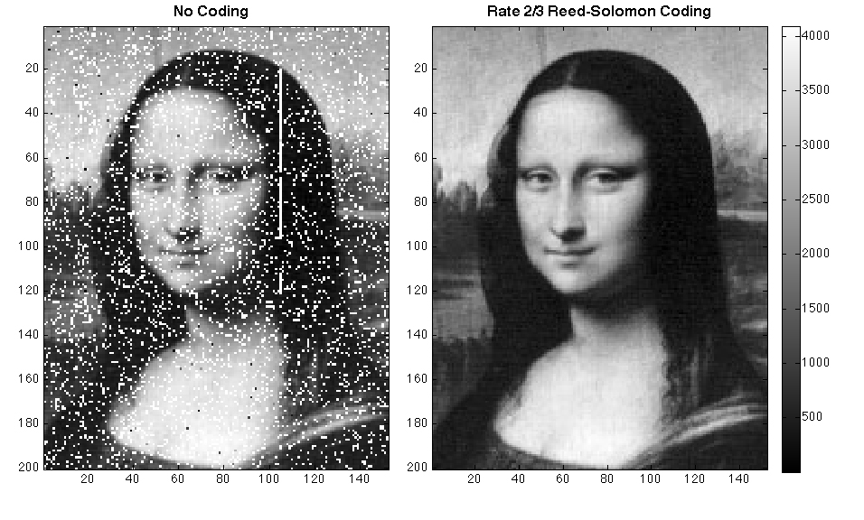
In this module, we will spend a lot of time talking about compression and error checking in our computers. We’ve already talked about compression a little bit in the data encoding module earlier this semester. But now we’re going to spend an entire module talking about just these two topics. First, we’re going to talk about in compression. What do you think compression is and why do you think it’s useful? As you might recall, compression is reducing the amount of space a particular piece of data needs to be stored on a computer. And if we think about that, that may not even really make sense, how can we take the piece of data and store it in fewer Bits and Bytes than what it originally was? It turns out, there are a lot of different ways to do that. We can do all sorts of different things by replacing repeated chunks of data or re-encoding the data in such a way that we can interpret it differently in our computer systems. And we’ll take a look at that in this module.
Why do you think we would do that? Well, computer resources are very expensive. For example, think about the storage space in your computer. While you might have a couple of terabytes. If you’ve ever played video games, or downloaded a lot of videos, you’ll find that that space gets eaten up very, very quickly by those large files. And so we can use compression to reduce the amount of space that those files take up and store them in fewer hard drives than it would take to store the raw files. Likewise, we can think about transmission bandwidth across the internet. If we need to send a large file across the internet. If our internet connection is very slow, it might be better to compress the file before we send it and then allow the other user on the other end to decompress that file when they receive it. However, of course, this does create a trade off, we’re spending computation time to compress and decompress the data in hopes of saving transmission time in storage space when we actually store or transmit the file. And so depending on the amount of computational power we have, and the amount of transmission or storage space we have available, it may or may not make sense to compress data. But in general, compression is usually a good thing and helps us save more data in a smaller amount of space, and transmit lots of data very quickly across the internet.
So let’s take a look at one example of compression called run length encoding. In run length encoding, we’re looking for runs or repeated sequences in our data. And then we’re going to going to replace them with a shorter version of that data in our actual store data itself. Usually that shorter version would be the sequence that we’re repeating, and account of how many times it gets repeated. So let’s take a look. Here’s an example of data that we could send via run length encoding, we’re using characters and recall of course, the characters can be stored as binary values using ASCII the American Standard Code for Information Interchange. So while we’re representing this data as text, it would actually be stored and transmitted as binary on our computers.
So in run length encoding, we would look for repeated characters and try and replace them with shorter versions of themselves. For example, if we look at these W’s at the top, we can see that they’re an awful lot of them. So let’s count them, we have 1 2 3 4 5 6 7 8 9 10 11 12, there are 12 W’s. So in our in our data, we would say that we have 12 W, then we have one B, so we just write one B, then we have 12 more W’s. So if you count those out, there will be 12, W’s, and so on. And so with run length encoding, we would be able to count the number of each characters and put a number followed by the character that shows up. So if we encode all of this data with run length encoding, we would get 12 W, 1 B, 12 W, 3 B, 24 W, 1 B, 15 W.
As we talked about earlier, the characters W and B can also be stored as binary. And of course, these numbers can be stored as binary. So it should be pretty easy to figure out how we can convert this particular string of data into a binary string that we would send along with our data.
But there might be a problem. If we think about all of that being one long string of binary numbers, how could we tell which parts of it are the numbers and which parts of it are text. And remember, the text itself is just numbers as well. So maybe we need to come up with some sort of a scheme that allows us to structure that data so that we know where the numbers are and where the text is. So let’s take a look at that.
Here’s that same example again, but how do you think we could write it so that we can easily tell which ones are the text and which ones are the numbers? Take a minute to think about that before you move on. A better way to think about this would be to use escape sequences. So in escape coding, what we would do is we would have a double character representing an escape sequence. For example WW; the WW being a repeated character would reduce down to just a single W. But then afterwards, we would have a number. And so looking at this bottom, we see WW followed by 12. The ww is our escape sequence saying we are going to repeat the letter W. And the next bit of binary data is going to be the number of times we repeat that character. So we see WW 12. Then we see just one B. And because B is not repeated, we just assume that that is text.
Next, we have WW again. And since that’s a repeated character, that will tell us that we’re going to repeat W and the next bit of data is going to be binary, that is the number of times we repeat that character. So then we have WW 12. Now we have three B’s, so we have BB 3. Then we have WW 24, a single B, then WW 15. So if you look at this, that is a little bit longer than the example we saw earlier, because we have to double some of the characters. But this example is much easier to read for our computer. We know that every character is text, except if we see the same character twice. And then we will know that the eight bits after that represent a number that we could use to repeat that character that many times. So now that we’ve seen an example of run length encoding, we’re going to let you give it a try in the next quiz.
Next, let’s take a look at another form of compression called Huffman coding. Huffman coding uses the frequency of the letters in a piece of text to reduce the amount of space that they take up in the encoded data. To do this, we will count the occurrences of each character in our text. And we’ll use that count to make a binary tree with the data. Then the paths of the tree to each character give the codes that we use for the Huffman encoded data. This is a little bit complex.
But let’s take a look at an example and see how this works. Let’s say we’d like to send this particular text using a Huffman tree. This is an example of a Huffman tree. If we count this just as plain ASCII characters, it would take 298 bits, which is 8 times 36 characters to send this data. So now let’s look at how we would encode it into a Huffman tree. The first thing we would do is we would count the number of occurrences of each character.
So let’s look at an example of how we would convert this into a Huffman tree. The first thing we would do is we would count the frequency of each character. So let’s take a look at the spaces we have 1 2 3 4 5 6 7. So we have seven space characters in this particular example, so we can make a list. On this slide, we see the list of some of the most common characters in that text. There are seven spaces, 4 letter A’s, 4 letter E’s, 3 F’s, 2 H’s, 2 I’s, 2 M’s, 2 n’s, and so on.
So with that data, we can then construct a binary tree by using the frequency of the characters to determine where they go in the binary tree. Since the space is the most frequent character, we’re going to put it at the very top of the tree, whereas least frequent characters, for example, a p would go toward the bottom of the tree. So if we follow the Huffman example algorithm, we’ll see that we create a binary tree that looks something like this. And this is pretty complex. And we’re not going to exactly talk about how to build this binary tree. But there is a very unique algorithm that you’ll learn about later on that can allow you to do this.
So now we look at this tree. And we see that the space character is way over here. We mark it for you. So the space characters right here. So to get to that space character, we will make right, here, right here, and right here. So the space character, in terms of directions would be RRR. Likewise, the E, we would go left, left, left. So E is going to be left, left left. This is the space, this is the E. And so in Huffman coding, we would use the direction that we go in the binary tree to become our data. So if we encode this, so that right is ones, we would do 111 for the space, for the E, it would be 000. Pretty cool, isn’t it?
Likewise, if we want to get to the letter A, we would go left, then right, then left, so A would be left, right left to get A. So that would be 010. Pretty cool, isn’t it. So we’ve taken characters that normally need eight binary values to represent them. And we can represent them here with this tree in anywhere from three to five characters. So if we look at this Huffman example, broken up, we’ll see something like this, the letter team becomes 0110, H is 1010. And if we go on, we can eventually find the A, which is going to be this one right here, th, this, space, is, space, A n, space, example, we saw that he was 000. So right here, we’ve got a really big improvement. We’ve gone from 288 bits of data all the way down to 135 bits of data. So we’ve nearly cut it in half a little bit more than half actually, to make this work.
Now, of course, Huffman trees do come with one particular caveat that we have to talk about. If we want to transmit this data encoded using a Huffman tree, we would also have to send a representation of the Huffman tree itself to allow this data to be decoded. And that can add a significant amount of overhead on small texts like this. In fact, the amount of data we would need to send this Huffman tree would be way more data than we needed to encode the original message even completely uncompressed. So while Huffman tree is a very powerful encoding system, It really works well when you’re sending large amounts of text like an entire book, then using a Huffman tree to encode that you can get significant savings in your compression. So once again, we’ve got a little example of the Huffman tree encoding problem that you can try on the next quiz.
Now let’s talk about error checking. What do you think error checking means when we’re talking about sending and retrieving data? And why do you think it would be useful? Well, let’s take a look at an example. When we send data, such as this text, hello there, sometimes the data might get garbled in transmission. When you were a kid, if you played with radios or walkie talkies, or anything like that, you might have had trouble understanding what other people say, Heck, even it happens today, sometimes on cell phone calls. So if there was a way that we could confirm that the data we’re receiving is the data that was actually sent without adding too much overhead to the data, that might be a really powerful tool, a great intuition to think of is squeezing the data into a smaller space, and then using that to check and see if we got the right answer.
So if we start with the text, hello there, and we squeeze the kerning, between the characters really narrow, we get this image shown below, that we can use as a little check to make sure that the data that we received was the same thing. So on the receiving end, if instead of receiving Hello, there we see Hello, ghere. If we squeeze that together the same way, we noticed that the squeezed image does not look the same as the squeezed image above. And so by sending the squeezed image above, we would know that we didn’t get the right data. And that squeezed image doesn’t take up a whole lot of space. That’s really the intuition behind error checking, we’re trying to send a little bit more data along with a larger transmission. And we can use that little bit of extra data to make sure the transmission itself was received without errors. That’s the real intuition behind this.
So let’s take a look at an example. One of the best ways we could do this is simply adding together the numbers. So if we take the sentence Hello there, and we convert it to ASCII, we see that a capital H is 72, e is 101, L is 108, and so on and so forth. So if we take all of those numbers, we could just add them up, and send all of that ASCII text plus the number 1101. Pretty cool, isn’t it, then on the receiving end, if the T got replaced with a G, obviously, the sum we would get would be different. And we would know that somehow that message got corrupted. Of course, this might be a little bit complex, for example, 1101 doesn’t fit in an eight bit binary number, so we may have to truncate it a bit or use modulo, to reduce it down to a number that fits into an eight bit binary value. Now, of course, this is a very simple form of error checking, and it does have some flaws. So let’s talk about some of these different questions. For example, if we only have the sum that came along with that message, could we use that to recover the original? So if I just gave you 1101? Could you tell me what original message produced that sum? Probably not. It would be really, really difficult to do. So we can’t use it to recover the original.
How well does it detect errors? Well, if we change the T to a G, we would probably detect that. But what if we replaced an L with an M and another L with the letter right before L? How well does this detect errors? Well, let’s consider the case where one of the L’s in hello gets replaced with an M, and the other L gets replaced with a K. M is one greater than L. But K is one less than L. And so when we sum those together, we would still get the exact same sum. So it is possible for us to create an error that the sum itself does not catch, that’s not really good. So as we can see, are the areas that cannot detect absolutely, we could swap characters, we could rearrange the characters, they would all still sum up to the exact same value. There’s tons of ways that we could do this. And of course, we talked about this a little bit already, but 1101 is larger than eight bits. How should we handle that? Well, we could use modular division where we divide it by 256. And keep the remainder, which would be the modulo operation that you learn about in your programming courses that would allow that number to fit in just eight bits. But of course, the big question we always ask in this class, can we do better. And I would argue that there are ways that we can definitely do better than a simple addition error checking.
So let’s take a look at another example of error checking. In this case, it’s called pinpoint error checking. Here, we’ve received a number 483754. So very large number, and we’ve taken that number and we’ve arranged it in a four by four grid. And then we’ve added a column in a row to the end of the grid that we can use to calculate what we call our checks up, which is the sum that we’re going to create to make sure that these numbers are correct. To create that checksum, what we will do is we will sum up each row and each column and then we will keep just the ones place of that value in this call. So for exam We have 4 plus 8 is 12, plus 3 is 15 plus 7 is 22. So here we would put 2, here we have 5 + 4 is 9, + 3 is 12, + 3 is 18. So we would keep the 8. Likewise, we could go down, we have 4 + 5 is 9, + 2 is 11, + 3 is 14. So we would keep the 4, here we have 8 + 4 is 12, + 2 is 14, + 9 is 23. So we would keep 3. And we could do this all the way through until we got all of these numbers, which we see right here, we see 4306 along the bottom, and 2858 along the side, then when we send the message, we could simply add those numbers in where they go, we see down here are 4837 of our original number, plus this 2 for our checksum 5436, plus an 82256, plus a 53397, plus an 8. And then we have 4306, which is our bottom checksum. So we have a 16 digit number. And we’ve added 8 more digits to it to provide a checksum. So it’s gotten a little bit bigger, it’s about 50%, bigger than it was.
But what can we do with this checksum that’s very, very powerful. So here, we’ve received a message. And we have in gray, our original checksum. And then in red, we have the checksum that we calculated from the message that we received. So take a look at this and see if you can figure out exactly where the error is in this received message. All right, let’s see if we can find the error. So we look at our checksum for matches up. 3…, uh-oh, this one doesn’t match up. So we’re going to circle this one. Zero matches up, six matches up, two matches up, eight matches up, uh-oh, here, 5 and the 0 don’t match up, and then the 8 matches up. So if we look at the row and the column, we know that this one is incorrect. Now the big question is, can we use this to restore that value to what it originally was, we know here that this value should be eight larger, or should be five larger, and we know that this value should be there, five larger five smaller. So with this number, if we add five to it, and just keep the ones place, we know that this number should probably have been a two. So let’s look at our original. Uh huh. It was a two. So using this pinpoint checksum by adding a little bit more data to the data that we’re transmitting, not only can we detect an error, but we can actually correct an error. And there are some different ways we can measure this. For example, we can detect a lot of different errors, but we may not be able to correct as many errors as we can detect. And that’s one of the important things to remember about checksum such as this. So now that you’ve seen an example, we’ll have a little quiz after this where you can do another example on your own just to see how this works.
The C2 total on the slide at 0:54 - 2:10 is incorrect. The total is 7336 but that value modulo 255 is 196, not 96 as shown in the video.
Let’s look at an even better way to do a checksum to check and see if our data is correct. This is called Fletcher’s checksum. And here we’re giving a quick pseudocode of the algorithm that is used to generate Fletcher’s checksum. Basically, the way it works is you divide the word into a sequence of equally sized blocks. And we’ll just use the individual characters for this. And we’ll start with two checksums, one of them, C1 starts at zero, the other to also starts at zero, then for every block, we’ll add the value of the block to the first check sum. And then we’ll add the new value of that checksum to the second checksum. And then finally, while we’re done, we will calculate the values of the checksum mod 255 to reduce them to an eight bit binary value. And we’ll return those two checksums.
So let’s take a look at an example of how we would do Fletcher’s checksum. We’ll start with our same messages always and divided into blocks where each character is its own block. So the first character, the capital H is a value 72. So we’ll add 72 to the first checksum. And then we will add that checksum value to the second checks up. So after the first character, they’re both the same. The second character, the lowercase E is 101. So we’ll add 101 to the first checksum to get 173. But now we will add this new checksum 173 to the value of 72 and the second checksum to get 245. Likewise, we’ll add 108 to 173 to get 281, then we’ll add 281 to 245 to get 526. And we’ll continue this process until we’ve done all the letters. And then at the end, you’ll see that we still get the same checksum that we found earlier 1101, which becomes 81 when we do mod, and then the second checksum becomes 7336, which is 96 when we do them on. So now we only have to send along two additional numbers along with our text. And that will tell us a lot more about the text in the errors. So let’s take a look at that and see how many errors this can find. Let’s consider the case of just doing these first three characters. So we know that the checksum for 72, 101 ,108. If we look back here should be 281 and 526. So we would have 281 and 526. So let’s look at this first example. We have 72 108 101. Well, that changed the first checksum? No, it’s the exact same value, it will be to 81. However, will it change the 526? Well, we start with 72. And then we will add 72 plus 108, which is going to be eight 180. So the second check sum will be 180. So we’re going to add 180 here, 180 here, which is going to be 252. And then to the 180, we’re going to add 101. So the second checksum is still going to be 281. But if we add 281. Here, we’re going to get 331, we get 533.
So in this example, by switching these two characters, the first checksum did not change, but the second checksum definitely changes. And that’s because the order changed. Likewise, when we look at all of these examples, we see that all of them add up to the same set of characters. So the first checksum will always be 281. But the second checksum will be different every single time. And that’s because we’re adding this first checksum to the second checksum every single time so it captures the ordering of the characters as well as the values that they may change based on those different values. So even by adding a zero in there, we would get a different value for that second checksum. So once again, there will be a quiz after this video where you can try a little bit of Fletcher’s checksum just to see how it works.
Let’s go over a couple other error checking methods that you might run across, we’re not going to go into these in too much detail because they are kind of complex at this level. But we’ll give you an idea of what’s out there, just so you can say you’ve seen it. One interesting example is the cyclic redundancy check or CRC. With CRC will have some sort of binary value. And we’ll use a particular checksum to verify it. So we’ll start with this binary value on a checksum. And we will compute the XOR of the checksum, and that binary value. So we start with 1010. And we XOR that with 1011. So we’ll get 1. And this works a lot like long division, we just keep working down the value until we get left with something that is smaller than our checksum. And so with this input 101000001001, we would send along these three bits 011 as our checksum. And then once we’ve received it, we can do this same division again, and make sure that we get the same checksum to know that the error hasn’t been introduced in our code.
Another method of error checking is hash codes. And hash codes are really complex. But they basically are a one way algorithm to take any piece of data and convert it into a single value. So for example, we would choose some sort of a hash base like 2 or 10, or 37. And then if we have a whole bunch of numbers, we would calculate the hash as the first number times our base to the value in plus the second number times the base to the power n minus one, and so on, and so forth. So if we have the word 456, if our base is 10, obviously, our hash should be 456. If our base is 100, we get 4056. If our bases, just five, it would be 126. But if we choose some interesting other numbers, we would get different hash codes. Later on, if you start taking programming courses, one of the data structures you’ll learn about is a hash table, sometimes known as a dictionary or a hash map. And to do that, what it does is it takes a piece of data and it computes the hash of that data, and then uses that to store the data in a unique way so that it can be quickly retrieved. But we can also use those hashes to verify data.
Another really common use of hashes would be password store. For example, md5 is a commonly used pass password hashing algorithm, or at least it was it’s been cracked since then. But you could take any text and calculate the md5 hash of that text and store that number. Then if anyone tried to input a password, you would simply take their password, re-compute the hash. And if it created the same hash as the actual password, then you know that that user inputed the create the correct password, and you could allow them access. Here’s another quick example of hash codes, just showing what it would look like for some other input data.
Another form of error checking you might run into is called a hamming code. And a hamming code is kind of complex. But what it does is it takes the data bits that you want to send and it calculates what are called parity bits for those data bits. A parity bit is basically a bit that’s designed to make all of those data bits plus the parity bit come up to an even number of ones. So if we want to send the data in bits, 3,5,6, and 7, for example, we want to send 0100, we calculate these three Hamming parity bits. The first one is 3,5,7. So we look at 3,5,7, there’s only a single one there. So that parity bit would be a one, the bits 3, 6, and 7 would be 3,6,7. There’s no one so we put a zero there. And then for 5,6,7, there’s a single one, so we need to add one more one to get to an even number of ones. Then to construct the actual hamming code, we have our first parity bit, our second parity bit, so one, zero, then we have our first data bit zero, then our last parity bit one, and then the last three bits of our data Five, six, and seven. It’s a little complex. But the concept behind Hamming codes is to create data words that are so far apart from each other that a single bit error, you can almost just round it to the closest binary value that makes sense for the hamming code that you’re using, and use that as your way to solve different errors. In this module, we’ve covered a lot of different ways that you can compress and do error checking on data that you send and receive or data that you store in your computer’s while a lot of this can be kind of complex and math heavy.
I’m hoping this opens your eyes a little bit to some of the things that go on behind the scenes on your computer that you might be aware of, but really didn’t understand how they work. We deal with things like zip files and JPEG images all the time. And those are all examples of compression. Error checking is a little bit more behind the scenes, but it’s really the backbone of how we can send and receive data across the internet using these unreliable connections and packets that might be dropped and still be able to recover and understand the data that we receive on the other side.
Nine Algorithms that Changed the Future Ch 1 - Introduction
Nine Algorithms that Changed the Future Ch 5 - Error Correcting Codes
Nine Algorithms that Changed the Future Ch 7 - Data Compression
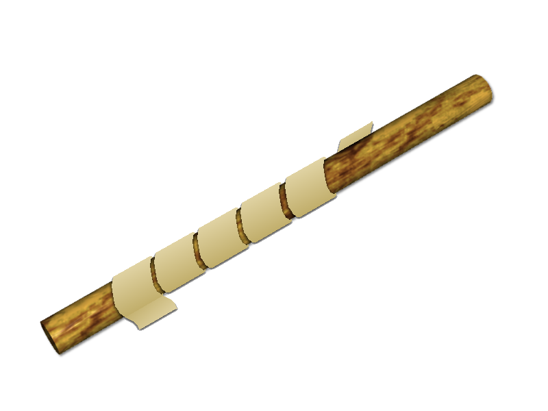
In this module, we’re going to take a look at one of the most important applications of computer science and modern technology- the field of cryptography. Cryptography is the study of ways to communicate securely and privately in the presence of third parties. If you think about it, cryptography is very important today with the rise of the Internet and modern technology. Any data that’s transmitted over the internet can be intercepted by just about anyone from your internet service provider all the way to the website that you’re communicating with, and anybody in between. Remember, the internet is built upon open standards, and so anybody can understand the packet formats and deconstruct them very quickly. So we need a way that we can encrypt and secure the data inside of those packets. So they can only be opened by the intended recipients, and that’s where the field of cryptography comes in. There were lots of historical Computer Science professionals interested in cryptography. Charles Babbage was very fascinated by it. Alan Turing was especially involved in cryptography, and Claude Shannon, were all involved in the field of cryptography. Also, surprisingly, the author Edgar Allan Poe was one of the people that was really excited about cryptography outside of computer scientists, and in fact, helped popularize cryptography as a word game that you might see in your newspaper.
So let’s take a look at an example of what cryptography might look like. When I used to teach this in a classroom, I would usually start by having strips of paper with this particular message printed out and laid all over the tables, and I would encourage students to see if they could decrypt this particular message. So on the slide here, you see the same text that I have written on the strip of paper, but it can be kind of hard to decrypt this message. So take a look at it and see if you can come up with what this message should say. I’ll give you a hint. If you have a marker nearby, or something that’s about this big and round kind of dowel shaped, that might help. Still need a hint? Well, what happens if I take this piece of paper, and I wrap it around the marker like so. Take it and wrap it. Just like that. So now I’ve taken this message, and I’ve wrapped it around the marker. And you’ll notice that when you do this, the text kind of starts to line up, you can see that there are characters that start to line up. That’s what this is. This message is actually an example of one of the earliest forms of cryptography called a Scytale. A Scytale was round dowel rod, kind of like this marker that you could use to encrypt and send messages. And it was used all the way back in ancient Roman and Greek times. For example, if you wanted to send a message to somebody, you could take a strip of leather and wrap it around the Scytale, and then you would impress the characters of the message across the strip of leather on the Scytale. Then you would unwrap it, and you’d end up with a string of random characters that look something like this on the paper, and you could send that piece of leather out into the field. And of course, the only way to decrypt it would be to know how to decrypt it, and to have a Scytale that was the same size as the one that was used to encode that message. And so if you were very careful, you can use Scytale of different sizes to encode different messages using the same technique. So if we start with this message in the class, you realize that a Scytale is really just an iterative cipher, where we start with about every six letters. So we have this is a Scytale example. That’s what that message would say. Now, of course, you’ll notice I’ve added the letter Q in there a couple of times. And that’s actually very commonly done in the field of cryptography. As long as the message is understandable to the person receiving it when they decrypt it, you can add some random characters in there that don’t make any sense once you have decrypted the message, but it can really help foul up people trying to decrypt the message and use every single character in the message. It’s a neat little trick to make your encryption just that much more unbreakable.
There are lots of examples of early ciphers that have been used throughout history, we looked at one called the Scytale. There are also things such as substitution ciphers. A substitution cipher is where you take the letters in your text and you simply replace them one for the other. For example, all B’s become Q’s. All K’s become G’s, and so on and so forth. If you read the newspaper or do puzzle books, you might have seen a puzzle called a crypto quip. That is actually an example of a substitution cipher, and it’s one that was made popular by Edgar Allan Poe. Of course, putting your crypto equipment in newspaper might lead you to think that it’s easily breakable, and it totally is. One of the best ways that you can break things that are substitution ciphers is by frequency analysis. You look for the most frequent characters, and then you assume that those would be probably the most frequent characters in the English language. For example, in English were helped out a lot by the game show Wheel of Fortune. We know that the letters R S T L N E are some of the most frequently used characters in the English language. So if we find the most frequent substituted letters in our substitution cipher, we can try those characters and see what works. Also things such as short words, two letter words, things like that really helped break a crypto crypt very, very easily.
So then you get to more advanced ciphers called polyalphabetic ciphers. And these are like substitution ciphers, but much, much more advanced. For example, you would substitute letters not only based on the previous letter, but the position and all sorts of other things. Polyalphabetic ciphers were first described all the way back in the ninth century AD by the Islamic mathematician al-Kindi, but they were later explained in a lot more detail by French mathematician Leon Battista Alberti in 1467. So of course, once again, polyalphabetic ciphers can seem very complicated. But once you really discover how many different substitution ciphers there are in a polyalphabetic cipher, then it reduces the problem to simply breaking each of those individual substitution ciphers one at a time. So while they’re still powerful, they’re not nearly unbreakable, like we might think today.
Another example of an early cipher would be the tabula recta. A tabula recta, like you see here is all of the letters of the alphabet are arranged in a grid. And you can see that each grid shifts by one letter. Then with a table such as this, there are a lot of different algorithms you can use to encrypt data. For example, you could use the previous letter in the data to encrypt the next letter that you want to encrypt. So if we want to encrypt the word HELLO, we would start by using H to encrypt H. So we get H, but then the next letter E would be encrypted using the H line and it becomes L, then we use the next L to encrypt L. So we would encrypt L, which would be W, then we use W to encrypt another L, which becomes H. And then we use H to encrypt O, which becomes V. And so by following that process through, we can use the tabula recta to create a very, very hard to break cipher just by following an algorithm. And of course, you can do all sorts of different things with this and it creates a pretty powerful cipher, not one that is completely undecipherable. But it’s a very powerful way to do something using a very simple table such as this. And this is actually the same basis of things like the decoder rings that you might have heard about that were sold in cereal boxes years ago, they use the same basic idea. If you have the table or the decoder ring or whatever the ciphers key is, then it becomes very easy to break but without the key, you have to discover the key in order to break it easily.
In this module, we’re going to take a look at one great example of the use of cryptography in computer science. And to do that we have to go all the way back in history to look at World War Two. This slide right here shows the height of German occupation of Europe during World War Two. And during that time, the Germans were sending encrypted messages to all of their field commanders using a system that was very, very much thought to be uncrackable at that time. So we’re going to take a look at what that system is, how it works, and how the Allies were actually able to crack it by taking advantage of some of the knowledge that they had about such a system. Oh, and of course, some of this information would have been very much top secret, and a lot of it was classified up until just a few decades ago. So it’s really an interesting time to take a look back at what was going on during World War Two, and take a look at how the Germans were able to build a very interesting encryption system that was then later broken by the allies. So let’s start by taking a look at a quick video demonstrating the German’s Enigma machine and how it worked.
Watch through 5:50
I present to you the German Enigma machine. The Enigma machine was used to encode messages during World War Two. And it was a really interesting piece of equipment. It used several different rotors that were rotated to create a key for the encryption, and used a plug board and a keyboard for inputs. And so as we saw in the video with the Enigma machine, you would set the rotors to a particular key. And then when you press the key on the keyboard, and electrical current would go from that key, through the plug board, through the rotors, back out through the rotors, and then light up a lamp above. And so by pressing that key and holding it down, it would show you the letter that that letter should be encrypted to. Then, you would press the next key, another letter would light up, you press another key, another letter would light up. And each time you press a key, the rotors would advance one click changing the way that things were encrypted. And so of course, if you sat there and kept pressing the same key on the keyboard, you would notice that every single time you did that the letters that it would light up would be different every single time making you think that this is a very, very hard to break cipher. And indeed it was.
So as we saw, the Enigma machine consists of several rotors. Each rotor has 26 letters engraved around the outside, and it has 26 pins, each pin representing the input for one letter. And so you’d have a pin on one side, a whole scramble of wires on the inside, and then on the outside, you would have another contact that would go out. And so each pin was paired to one contact, but they were shuffled around randomly, so you really didn’t know how it was set up. And so of course, with just three rotors in the Enigma machine, that means there are over 17,000 possible combinations of three character positions of the Enigma machine rotors. So here’s an exploded view of showing the between the rotors where you have the pins on one side, making contact with the contacts on the other side. And so by sending an electrical current through one of the rotors, it would eventually go through the pins and contacts through each rotor until it would come back out the other side. And then of course, like we talked about, the Enigma machine uses a ratcheting system, very similar to an old analog odometer in an old car. Every single time you press a key, the ratcheting system would advance the outermost rotor, one click. And then of course, once that rotor has made a full cycle, it would advance the second rotor, one click, and then once that outside rotor has made 26 cycles, and the inner rotor has made 26 cycles as well, then the first rotor will be incremented one click. And so like it works just like an odometer, it’s very, very interesting the way they set this up.
But probably the most interesting fact is the way that the reflector works. So for example, let’s say you press the letter A on your keyboard. Then, it would go through the right rotor, the middle rotor the left rotor, and it would hit this special plate on the other end called a reflector, which would take that input on one pin and it would output it on another pin. Then it would go back through the rotors using a different path, and then it would hit the letter G and light up that light. But this right most rotor would then advance one position. So the next time you press the letter A, you would get an entirely different combination. You would have A which would go through this path, hit the reflector, come out this path, and then it would light up the letter C. So this makes decrypting messages really, really impossible. You never know what letter you’re going to get out based on the inputs unless you really know everything about how the position is set up. Finally, on the front of the Enigma machine, they included what’s called a plug board. And so what the plug board could do is you could swap the positions of two letters using these little wires. So for example, this system is set up to swap the letter S with the letter O and the letter J with the letter A. And so with this plug board, you can have up to 13 swaps, which gives you 10 million different combinations of keys that you might have to worry about. Of course, it’s interesting to note that the swaps are reflexive, so if J gets swapped with A, then A also gets swapped with J, so the same happens for both letters.
So all told, you have all sorts of different ways to set the key for the Enigma machine. You have the choice of the rotors and the ordering of the rotors. We saw three rotors, but toward the end of the war, there might have been as many as eight different rotors available that they could use. Then you have the initial position of the rotors. So the initial three letter key that the rotors were set to. You have the ring setting on the rotors, which shows where the rings go on the rotors, that way, it kind of changes the position a little bit more. And then you’d have the plugboard connections on the front, which are swapping different letters around. And so in theory, to understand how an Enigma machine is encrypting data, you would need to know all four of these things for each Enigma machine that you want to try and decrypt. And that’s a lot of information to keep in mind. Now of course, the other thing that they did is they had a specific operational pattern that they use when they were encrypting data using an Enigma machine. So the first thing they would do is they would set the wheels on the Enigma machine to the key from today’s codebook. The Germans carried around these code books that gave the keys for each day. And unfortunately, throughout the entire war, to my knowledge, not a single codebook was lost. In addition to the key settings, there was a particular way that the Enigma machines were operated. To operate an Enigma machine. First, they would set the wheels to the key from today’s codebook, the Germans used a paper codebook that gave different keys for each day of the year. And to my knowledge, those code books were not ever compromised during the war, they would always be burned or destroyed before any German camps were taken over. Secondly, the operator of the Enigma machine would then choose a unique key for the message. So they would choose a different key consisting of three characters for that message. So then they would use the daily key to encode the message key twice to avoid errors. So the first six characters of the message would be the message key encoded twice, then you would set the wheels to the message key, and start en crypting and sending the message. So not only did each day have a different daily key, but then each individual message used its own message key to send the data, so everything was really scrambled.
So if we look at this process, how do you think you’d go about cracking an Enigma machine? Take a minute to think about that. So obviously, the Enigma machine had many strengths. There were many different factors to the encryption, as we saw earlier. There were eight different wheels to choose from by the end of the war. And so depending on how you calculate it, there could be as many as 150 trillion different setups just from the plugboard itself. So altogether, it’s estimated there were 158 quintillion possible keys that you could use to decode an Enigma machine.
However, the Enigma machine came with very, very important weaknesses. The first and most important weakness was a letter would never encrypt to itself, because of the way the reflector worked on the plug boards and on the wheels. If you press the key A, you could press that key 26 times, and never once would the light for a light up because they were on the same circuit. And so with the reflector through the wheels, there was no way the current could come back through the circuit that it was sent out, which means that A would never light up for itself. Secondly, of course, the plug boards were reciprocal. And so by swapping two letters, you’re really just adding a substitution cipher on top of a really complex polyalphabetic cipher so the plug boards really didn’t do a whole lot in terms of making the combinations more complex, it just scrambled the letters a little bit. Another big problem they had was the wheels themselves were not similar enough, the wheels were so different, in fact that using some advanced mathematics, you could determine roughly which wheels were being used, just by the way the letters were distributed in the message that you received. And then of course, there were some poor policies and procedures around the Enigma machine. And one of the worst parts was the fact that they allowed message operators to choose the key. If your message operator in a foxhole during a war, and you’re asked to come up with three random letters all the time, every time you want to send a message, are those letters going to be truly random? Or are you more likely to pick some letters that have specific meaning to you like the initials of your loved one back home or your hometown, and they actually found out that that was a problem. A lot of German message operators were not picking truly random letters for the message keys. And then of course, they were encoding those same letters twice at the beginning of the message. So if you could decrypt the first three letters of the message, you had the message key that you could then use to decrypt the rest of the code. So that was not really that useful. So now let’s take a look at a second part of this video about how to decrypt a message that’s encoded with Enigma machine.
Watch through 2:40
The success for cracking the Enigma machine really comes down to the work of this man, Marian Rejewski. Marian Rejewski was a Polish mathematician who worked on the Enigma machine in the early days of the 1920s and 1930s. The Enigma machine was actually originally available as a corporate machine; you could go out and buy it as a corporation, and use it to encrypt and store data. And so it wasn’t until much later that was taken over by the German Nazi Party and used in their war efforts. And so public Enigma machines were available and could be studied. And so Marian Rejewski was able to study some of the early Enigma machines and try and predict the adaptations that Germany made as they move closer to war in the late 1920s and 30s. So based on his work, he was able to determine what the Germans were doing and was even able to eventually replicate some of the German machines that they had created. But of course, that was just part of the story. So to crack the Enigma machine, it was really first cracked by Marian Rejewski of Poland. He was able to use some of those publicly available Enigma machines to crack some of the earliest things that they did. By 1938, as Germany was getting closer to war, they added two new wheels of their own making it much much harder to crack if you didn’t know the wheels existed. And so Marian Rejewski of Poland contacted folks in England and gave them a lot of his research and ask them for assistance. And so by 1939, Alan Turing, working together with the folks at Bletchley Park, created what he called the Bombe, which was a machine that could decrypt the Enigma machine. And so work on the Bombe progressed pretty much throughout the entire war. And by 1945, almost every single message that the German sent using the Enigma machine, could be deciphered by the allies within two days. So what is the Bombe? The Bombe is a machine developed by Alan Turing to simulate hundreds of Enigma machines side by side. You can see that it has all of these sets of three wheels, simulating the three wheels that might be present in an Enigma machine. And it was designed to explore many of the weaknesses and other facts about the Enigma machine that were known to the Allies based on the work of Marian Rejewski and Alan Turing at that particular time. So let’s take a look at a quick video of a Bombe in action just to see what it looks like.
Of course, the impact of cracking the Enigma machine cannot be understated. It’s probably best put by Sir Harry Hensley, who is a British intelligence historian. And he wrote, “My own conclusion is that it shortened the war by not less than two years and probably by four years … we wouldn’t have in fact been able to do the Normandy landings, even if we had left the Mediterranean aside, until at the earliest 1946, probably a bit later.” So really, the ability of the Allies to decrypt and decode the German messages sent via the Enigma machine was really important toward ending the war effort. And it’s almost unfathomable to imagine how bad World War Two had been, had it gone on for two or even four more years. And, of course, this is just focusing on the work in the European Theater. There was also another program called Ultra. It was based in the Pacific Theater, focused on decrypting some of the Japanese messages that were sent during World War Two. And so later on, we may add some videos to this module discussing that program, as well.
But let’s move into modern days and talk a little bit about Claude Shannon again. We’ve talked about Claude Shannon several times in this class before, but one of his most lasting claims to fame is as The Father of Modern Information Theory. And his work after the war really helped build the modern cryptography systems that we use today. He realized that there was a very mathematical way that you can encrypt data so that it could be very, very difficult to decrypt that data without understanding the keys used to build it. So because of a lot of his work in the 1950s, we refer to Claude Shannon as The Father of Modern Information Theory.
So one of the modern forms of encryption is called symmetric key encryption. And in symmetric key encryption, we take some sort of data such as the plain text hello world, and we encrypt it using a very particular algorithm and a key. And so the algorithm uses the data that we want to encrypt and the key, and it will produce what’s called ciphertext. And so the ciphertext is the encrypted form of the data that we can send and receive and do everything we want. And then to decrypt it, we would use the same key and sometimes a similar algorithm or a slightly different algorithm to get back to the plain text. So symmetric key encryption does have some advantages and disadvantages. One of the biggest things to remember with symmetric key encryption is that it uses a shared secret key. Both the person encrypting the message and decrypting the message need to have a copy of the key. And so that creates this interesting problem of how do we share the key without knowing that someone else got ahold of the key. And likewise, if we encrypt something with a shared key, and the other person has lost that key, then we may not know who has access to that data, making it really kind of complex. However, shared key encryption and symmetric key encryption does still get used from time to time. Most of the time, it’s used for file encryption, things like encrypted zip files, usually use symmetric key encryption. You use the same password to encrypt them as you use to decrypt them.
The other form of modern encryption that we’ll talk about is public key encryption. And public key encryption is a little bit more complex because it uses two different keys. So we start by generating two keys, a public key and a private key. The private key we keep for ourselves; we don’t give that to anybody else. A lot of times the private key is unique to a particular computer itself. Then we would give our public key to anybody; it’s public. We could tattoo it on our forehead. We really don’t care because that’s the public key. Then, anybody that wants to send us encrypted data, could take their data and lock it using the public key that we have made public available. And as soon as they lock it with that public key, the only person that can unlock it is the person with the matching private key. And so if they want to send something that only we can read, they lock it with our public key, and then we can unlock it with our private key. Likewise, we can go the other way, if we want to send something out to the world and have the world know that it came from us, we can lock it with our private key and post it out on the web along with our public key. And so anybody that wants to can look at that data, unlock it with our public key. And as long as they trust that that’s our public key, they know that we are the only person that could have sent that message. This is how things such as email signatures, the actual like signed signatures work. You can also do this on websites. If you look at your websites, they’ll have a lock that usually says it’s encrypted. And part of that is that the data is encrypted, but also part of that is that it’s verified that we know where that data is coming from using a process based on public key encryption. And then of course, we can combine the two. For example, if we’re sending our credit card data back and forth with a website, we can use their public key, and they can use our public key in very unique ways. For example, if we want to send our credit card data, what we could do is we could lock it using their public key so that they are the only person that can read it. But we can also sign it with our private key so that they know that the only person that could have sent that data is us. And so by combining the two, we can get both protected data, and we can get it signed and verified so we know where it came from. So let’s take a look at a quick video on Diffie-Hellman key exchange, which is how we can actually share keys back and forth and make sure that both users have a key that they can use to encrypt data.
In the video, the values of d and e are swapped at one point. Thankfully, this doesn’t matter since they are commutative and can be used in any order, but it is a bit confusing. We’ll correct this video in the future!
Let’s take a look at one modern form of encryption called RSA encryption. RSA was developed in 1977, and it was named for the three creators- Ron Rivest, Adi Shamir, and Leonard Adelman. RSA encryption uses the product of two large prime numbers to generate a key that’s used to encrypt data, and the strength of the key really depends on the difficulty of factoring that large number back into its two prime numbers. So for example, if we say our key number is 1071. Can we factor that into the two prime numbers? We could do it eventually, but we’d have to check a lot of different numbers to see what it was. So now imagine that 1071, instead of being a number with just four digits, was a number that had 64 digits in it. That’s really the size of the prime number products that we’re talking about when we do RSA encryption. And so really, the key to RSA encryption is the fact that it’s very, very difficult to factor a large number like that into the two unique prime numbers that are used to create it. So let’s take a look at how RSA encryption works to see why that’s important and why it can create a system that is easily broken if that rule doesn’t hold.
So for RSA, we start with two numbers, p and q. So I’m going to start out with p is five, and q is 17. So we’ve created two distinct prime numbers five and 17. Next, we will compute their products. So the product is n, which is equal to p times q, which is five times 17, which is 85. The other thing we’ll need to compute is Euler’s totient. And the totient of two prime numbers is actually just the number minus one. So to calculate Euler’s totient t, we would do p minus one times q minus one, which is going to be four times 16, which is 64. So we have p is five, q is 17, n is 85, and our totient t is 64. So let’s write that here. Again, we have p is five, q is 17, n is 85, and t is 64.
Now, here’s the really complicated part. We need to choose the number e less than t that is coprime to t so that they share no common factors. Then, we calculate d as the modular multiplicative inverse of e. So that e times x is equal to one mod t. This is really complex mathematics, but what it really means is we need to pick a multiple that is one more than a multiple of t. So if t is 64, we’re looking at 65 129 193, etc. So we’re finding multiples of t, 64, an adding 1, 65. 64 times two is 28, so 129. 64 times three is 193. 64 times four is 256. So we’d look at 257, etcetera. And then we choose one of these that we can factor. So let’s look at 65. Can we factor 65 into two numbers? It turns out we can. So if we set d equal to five, and e equal to 13, we get 65. And e is less than t, and it’s coprime to t. Specifically, e is prime, which is great. Two number are coprime if they don’t share any common factors other than one. And since 13 is prime, it’s also coprime to any other number, which is what we want.
So now we found d and e, which are the keys that we actually need to send and receive our ata. So let’s look at our RSA keys. We have two keys, our public key, which is going to be n and remember and n is 85 and e is five. And then we can encode using this, and we have our private key, which is 85 and 13. So let’s take a look at an example to see how this would work. If we want to encrypt the message 42, what we would do is we would take 42 to the power of five, and then we would do mod 85. So remember, the modulo operation means we divide by 85 and we keep the remainder. So if we actually do this on a calculator, you’ll find that this is equal to 77. And if you have a calculator handy, you can try this yourself. So 77 is the message that we can send as an encoded message. On the receiving end, we would take our encoded message 77, raise it to the power of 13, mod 85. And sure enough, if you calculate 77 to the power of 13, and you might need Wolfram Alpha to do this, then mod 85, you will get back the original message 42. That’s how RSA encryption works. It’s really, really simple. It’s mathematics with a little bit of flavor on top of it to make the keys.
Now, here’s the really tricky part. How do we break RSA encryption? Well, let’s take a look at our keys. Right here in both our public key and our private key, one part of that key is 85. What was 85? Remember that 85 is equal to our two prime numbers, p and q multiplied together. And since p and q are both prime, there is only one way that 85 could be factored. There are no other possible factors. And we know that we use five and 17. So if anybody can factor 85, into five and 17, then they can create t, because t is going to be four times 16, which is 64. And then using t if they have either e or d, they know that e times d would be one more than a multiple of t. And once they have that they could deduce the other half of the key. That’s what’s really important here. So RSA only works if this particular operation is very, very expensive. So to do RSA encryption, we choose numbers p and q, such that they are very, very large. And like I said, we’re talking hundreds of bits, we’re talking multiple digits long, and that’s why there’s so much computing power spent on the search for larger and larger prime numbers. Because for RSA encryption to work, we need those larger and larger prime numbers in order to construct RSA keys that we can use to send and receive data.
This is also really important later on when we talk about concepts such as computability. For example, we’re making an assumption here that the only way to factor a very, very large product of prime numbers is trying all possible prime numbers less than that number. So it’s simply brute force. Now, if we wake up tomorrow, and some mathematician has devised a better algorithm for factoring large products of prime numbers into their two primes, then all of the RSA encryption on the internet isn’t as secure anymore, because now there’s an algorithm that can do that quickly. Another fear would be that quantum computers could do this. And so if a quantum computer discovers a way to factor large products of prime numbers very quickly, it could have the same effect on RSA encryption. Now, of course, this is just one example of one encryption algorithm, but it gives you an idea of the fact that modern encryption is really built upon these ideas that there are very difficult calculations for somebody else to make if they don’t know the original numbers, but those calculations can be made very quickly for us if we know the original numbers that we used to build that key. So I hope this has been really informative. I really encourage you to try RSA encryption for yourself. It is very fun to do the math behind this. And just to see that it works exactly like you’d expect. You can go back and pick any two prime numbers for p and q, and go through this process. The hardest part is finding e and d. But there’s some really great helpers online that you can use, and I’ll link to one of those after this video so you can play around with RSA encryption yourself.
Nine Algorithms that Changed the Future Ch 4 - Public Key Cryptography
Nine Algorithms that Changed the Future Ch 9 - Digital Signatures

In this module, we’re going to discuss a lot of topics related to cyber security. Cyber Security is another important research area in computer science, and it’s one that directly impacts a lot of computer users in their daily lives. So in cybersecurity, we really are asking ourselves one big question, how do we keep our data secure, and that’s really all it comes down to. We’re trying to secure data both on our computers, but also as we transmitted across the Internet, and any other communication technologies we might be using. And so we’re going to talk about some different ways that we can keep our data secure on our computers.
Before we get into that, a word of warning, I’m encouraging each of you to put your white hat on when we talk about this. So in computer science, we talk about different types of hackers. And typically, you have the black hat hackers, which are the ones that do so maliciously. But you can also have white hat hackers, which are hackers that use their skills for benevolent means– to help companies find security holes in their infrastructures and hopefully patch those holes and become a little bit safer. And so some of the things we’re going to talk about today, if used maliciously, could be very illegal, they could be felonies, they’re very, very dangerous things for you to use maliciously. But as a computer scientist, it’s important for you to understand those topics so that you can defend against them and know what they are in case they get used against you. And so I’m encouraging us all to put our white hats on at this point, and come at this topic from the view of doing this for the good of everybody else and trying to help them secure and protect their data. Okay, let’s get started.
First, we need to talk about authentication. Authentication is a very, very important part of anything in cyber security. And authentication mainly deals with a few things, it’s determining if the person is who they say they are. So when you sit down to a computer, and you type in your password, that is a form of authentication. You’re letting your computer authenticate the fact that you are who you say you are. Now, typically, authentication requires three different factors. There are ownership factors, which is something the user has. For example, an ownership factor could be a physical key to a building, it could be a USB drive that has a token on it, or it could be some other symbol or some other device that the user has to authenticate that they are who they say they are. A police badge, for example, is a form of authentication that authenticates who that person is. The second one we can talk about is knowledge factors. A knowledge factor is something the user knows that authenticates themselves. Typically, we think of this as passwords and pin numbers or anything else the user has memorized. But it could be even other facts such as birth dates, and mother’s maiden names, and social security numbers, things that the user would know very quickly. Those are what makes up a knowledge factor. And for most computer systems, we use knowledge factors as the primary form of authentication. The third form of authentication is an inherence factor. And an inherence factor is something the user inherently is. An inherence factor would be things such as a retinal scan, or a fingerprint scan, or DNA test, something that these are really can’t change about themselves.
And so to authenticate a user in a computer system, we typically use one of these factors at a minimum to authenticate them. There is also something called multi factor authentication or two factor authentication, which you’ve probably come across, especially if you do online banking or play certain video games. And that is pretty much exactly what you think it is, it is two different factors of authentication combined to provide greater security. And typically, they combine something the user knows, such as a password or a pin number ,with something the user has, such as a credit card, or in a lot of cases, it’s access to a mobile phone or an email account. And that is something the user has or possesses as the second factor of authentication. So think about some places that you run into two factor authentication, video games, online banking. At K-State, a lot of faculty and staff now use two factor authentication whenever they authenticate at K-State. But a big question to ask yourself is, would you as a student like to have two factor authentication on your K-State account? Why or why not? Do you think it’s worth the extra security to really protect all of your important academic records? Or is it just an extra hassle if you have to get your phone out every single time you want to log in? Currently, for faculty and staff, we log in with our phones, but then we can have it remember our device for up to 10 days before we have to do that two factor authentication again. So it’s a little bit extra hassle, but it’s not super inconvenient if we’re using the same computer day after day. But I could see if you’re using lab computers and have to authenticate every single time, that might be a little extra hassle for you. So it’s something to think about.
So in this lecture, we’re going to hone in on one of the most common authentication factors, which is the use of a password. A password is a very traditional system used to authenticate users on computer systems, on websites, just about anywhere. But I think there’s a lot of misconceptions about how to make secure passwords and how secure passwords really are. And so we’re going to rely on some information to really look at passwords and how they can be made more secure and some of the ways that they may be are less secure than we thought. So this is a comic from XKCD. It’s one of the great comics that he does. And here, he’s talking about how we make a particular password. And we’re going to come back to this comic. But here he shows a pretty common password, we start with an uncommon, but non jibberish word, then we add like a number and a punctuation because almost every website, you need to have at least a number and a punctuation. And we do some common substitutions from leet speak so zeros for O’s and fours for A’s. Usually we have caps and 99% of the time, if you’re going to capitalize the letter, it’s going to be the first letter of your password. So what we have is we have a password here that has a few different bits of entropy. And in fact, if you calculate it out, there’s just about 16 bits of entropy in this box. So that means that there are roughly 65,535 different ways that you could build a password. Based on these rules. You choose a word, you add some numbers, and punctuations, and substitutions and things. And so 16 bits of entropy, that sounds pretty powerful.
But how would we go about cracking this password? What would that look like? So let’s look at some different ways you could possibly crack this password. Obviously, the first thing you could do is you could try brute force. You start with aaaaaa, that didn’t work aaaaab, that didn’t work, and so on. And so brute force hacking does work in certain scenarios, especially for things like combination locks. If you’ve ever done a an escape room, one thing you might realize is they give you those combination locks with four dials on it. And hopefully, you’re smart enough to realize that if you only get three of the four dials, and you can’t quite figure out the fourth one, you could brute force it in about 10 seconds. So you really don’t have to get all of the dials, you can just brute force a little bit. And so with combination locks and things, sometimes it’s very, very easy to brute force them. And in fact was simple passwords like old websites that required your passwords to be eight characters or less, you could actually brute force a password very quickly. For example, here is a six character password, there would be about 308 million different six character all lowercase passwords. It seems like a lot, but if we try it about 1000 a second, which is pretty, pretty common. I mean, even on a bad website, you could try 1000 passwords a second, it would only take us about three and a half days to crack that password. And in the grand scheme of things, three and a half days is not that long.
So let’s look at another way. How about things like rainbow tables. For example, this slide shows the 25 most common passwords used on the internet, according to some research done by Gizmodo a few years ago. And looking at this list, it is pretty disappointing. You’ll see passwords such as 123456, or 123456789. But you’ll see things like sunshine, qwerty, iloveyou, admin, abc123, certain profanity words. And so these passwords are really not all that great. And in fact, it’s really easy to go online and find some of the most common passwords that are available. Another thing that we can look at is what’s called rainbow tables. And so a rainbow table is actually a password lookup table that is calculated all of the protected versions of these passwords. For example, on older versions of Windows, when you set your windows password would actually be stored in the Windows registry using a hash. And so a hash, if you remember from our previous module is an algorithm that takes a piece of text and converts it to a number using a one way algorithm. And so the theory is if you type in the same password and go through the same hash algorithm, if you get the same output, you know, they put in the right password. But of course, what you could do is put in all possible passwords and store all of the possible hashes and create a table that matches them up. And so that’s what a rainbow table is, it basically creates a rainbow of all the different possible password combinations and the hashes that those create. And so if you have a Windows computer, an older Windows computer and can get the password hash out of the registry, you can go online to these websites that have rainbow tables and just put in that hash, and they will look up the password for you or at least a password that creates that hash. And so for a lot of really bad algorithms such as the early windows algorithm, there are some algorithms such as MD5 that rainbow tables are created for, you could just go out and look up a password based on a hash.
So between brute forcing common passwords and rainbow tables, there are a lot of different ways that you can crack really easy passwords. So let’s go back and look at that password example we saw earlier and talk about entropy. So he calculates that there would be about 28 bits of entropy in a common password there and 2 the 28 to get about three days at 1000 guesses a second. It’s really similar to what we saw with brute forcing, even though it’s a much longer more complex password, but it’s actually pretty easy to break a password like that. Now, here’s the hard part. Can you remember what that password was on that slide a few minutes ago? Don’t Look, don’t rewind the video and look, but see if you can write down that password that we saw earlier. Did you get it? Now you can go look and see if you got it. And so it turns out that we’re creating passwords that are really easy to actually crack if we understand the structure of the password. But it’s very hard for us to remember is it’s troubadour with an & and a three, but I don’t remember exactly what order so it’s hard to remember.
And so what he’s arguing here is we’re creating passwords that are basically easy to crack and hard to remember, what we really should focus on is creating passwords that are hard to crack, but easy to remember. How do you suppose we would do that? It turns out that to make more complex passwords, there is exactly one rule that you need to follow. And that is make them longer. That’s it. No special characters, no capitalization, punctuation, lowercase, uppercase, numbers, symbols, foreign words, does not matter. The only thing that matters to make your password more secure, is making it longer. So here we have four random common words, you start with 1000 common words in the English language. So that means you have about 10, or 11 bits of entropy per word. And you pick four of them correct horse battery staple. purple monkey umbrella dishwasher. very, very simple. All you have to remember is those four words, and I can even go out there and say, here’s a list of 1000 words. And my password is four words separated by spaces. And that right there would have 44 bits of entropy. So even if I gave you the list of words and told you exactly how my password was set up, it could take you 550 years to try all possible combinations of that password at 1000 guesses a second. That is much, much harder to do. But it’s very easy to remember, you probably already remember that password correct horse battery staple. It’s very easy to remember.
And so the whole idea behind making secure passwords, we see a lot of websites today that tell you you have to have a number and a symbol and special characters and whatnot, doesn’t matter. The only thing they should do is set a minimum password requirement of 20 or 30 characters and just tell you to make a long password. That right there will make your password more secure with a big asterisk on it. Understand that when we talk about security here, we’re only talking about security based on cracking the password using some sort of brute force method or some sort of dictionary based method. We are not saying that that password is secure against all attacks, for example, correct horse battery staple, if you write that down on a post it note and stick it under your keyboard, it would only take somebody about two seconds to read that password off of the post a note and remember it instantly. There’s nothing special about it. And so just because it’s easy for you to remember doesn’t mean that wouldn’t also be easy for someone else to remember. Likewise, if you don’t pick four random words, if you pick four words like your four grandparents or something like that, like their names, that could be much easier for people to crack. And so while it’s uncrackable from a computer standpoint, there are other parts of cybersecurity that we’ll get into a little bit later that make this password maybe less secure than what you want.
So finally, let’s talk about storing passwords securely in your applications. And there are a lot of different ways you can store passwords so that users could use them to authenticate. Let’s take a look at that. First, obviously, we could store the password itself. The user types in a password, we store that password in the database. Great, right? They type that password in again, we check it to make sure they typed in the same password. If they did, they let them in. That sounds like a really great system, doesn’t it? Hopefully, you’re cringing a little bit thinking about this. Because obviously, websites that have databases on them get hacked all the time. And if a hacker gets access to this database, they have your password. Simple as that. There’s nothing that they have to do, there’s no decryption they have to worry about, they get your password. And of course, one of the weaknesses of people on the internet is we tend to use the same password over and over again. Raise your hand, if you do that. I do. I use the same password a lot of places on the internet, it’s something I probably shouldn’t do. But I do. And so if somebody gets one of my passwords, they might be able to use that password to log into other websites that I use that same password on. So this is obviously not very secure. And the only thing that they need to compromise this is database access. As soon as they access the database, they have all the passwords, and it’s really simple so we probably shouldn’t do this.
What if we store the passwords by encrypting them using a key? Well, that makes them a little bit more secure, which means now if you get the database, you also need to have a key to decrypt the passwords, or of course, some sort of a lookup table or a rainbow table to decrypt the passwords. And so you know, as soon as they get the database in the key, it would compromise all the accounts. So this is better than storing the raw passwords. But it’s still not great. And it’s not that hard.
The really best way to store passwords is using what’s called a password salt. And this is because users are generally bad at creating good passwords. And so what we can do is take their short, crappy passwords and add a long string of random characters to it before we encrypt it. And so that will make the encrypted password much much stronger, it will feel like a longer password, even if the user’s portion of that password is very short. So it protects against all sorts of things like dictionary or rainbow table attacks, Rainbow table attacks assume that passwords are pretty short. Most rainbow tables only work on passwords that are 10 characters or less. So if we add a salt of 25 characters to the end of a password, we’re guaranteed to get something that’s pretty long and hard to break using just standard encryption attacks. So if we store with a global salt, which means that we use the global salt value, the same salt value for all passwords, then a hacker would have to get the database, the encryption key we used, and that global salt value. And the nice thing is those are typically stored in three different places. The database is stored, obviously, as the database. The encryption key is probably stored somewhere in the software, and the salt value is probably stored somewhere in the software’s configuration. And so you need to get all three of those parts to break these passwords. If you didn’t have the encryption key or the salt value, you could try and brute force it, but it would take a long time. The downside is once you brute force a password, you could get the key and the salt and use that to compromise all the other accounts. So if you get one, you still get all the accounts compromised, but it is a little bit harder to do. The other thing you can do, of course, is you can encrypt all the passwords with a unique salt value. So every single user, every single account gets its own salt value. And if you do that, you need the database encryption key and the salt value for each user account in order to crack it. And that makes it even much harder. That means you can only compromise one account at a time, because every single time you need to get that salt value for that account. And so that makes cracking these passwords really, really hard to do.
So lastly, let’s take a look at one of the instances where people have really broken passwords very, very quickly. And this is from the Adobe hack from several years ago. And again, this is an XKCD comic. But what happened is Adobe misused an algorithm called block mode ds. And what that does is every block of your password gets chunked up. So every eight characters or so it gets broken, and it gets encrypted separately. And because they did that incorrectly, if the user had the same password in that first eight characters, it would encrypt to the same thing. And so what you end up with is basically the world’s largest crossword puzzle. So for example here you would have weathervanessword and then you have name one. If you’re a fan of redwall, you might understand that weathervanessword might have something to do with Matthias from redwall and so this might be Mateus1. Here you have favorite of the 12 people apostles - Matthais, and then you have all these other ones like alphaobviousmichaeljackson. I’m guessing this is ABC123- the famous Michael Jackson hit from when he was in the Jackson5. It’s an obvious password, and it’s alphabetical. So there are lots of different examples of bad passwords, being stored improperly not correctly salting and hashing them like you should and this is one that Adobe definitely got called out for back in the day. So finally, if you want to take a look at your own passwords and see how secure they are, there’s this website howsecureismypassword.net. You can go online you can type in your passwords and it will give you an idea of how long it would take to crack that password.
Another area of cybersecurity that we should discuss is social engineering. Social engineering is all about using techniques to compromise the system by exploiting the users directly instead of the system security itself. And this is a really important concept. There’s an old saying, in computer science that a system is only as secure as the users that use that system. It’s kind of a play off the idea of a system is only as secure as its weakest link. And in most cases, the weakest link is the user itself. And so on the next few slides, we’re going to take a look at some different ways that you can use social engineering, to maybe break into a computer system and what those things look like so that we can defend against those. So a great example of social engineering is trying to get some information from somebody that they don’t want to give. And a great example of that would be a bank account number. So if I wanted to get someone’s bank account number, how do you think I could go about that using social engineering? Take a minute to think about it. So while this example may not work that well in today’s world, because not many people carry around checkbooks. If you have a checkbook, look at your checkbook at the bottom of your checks, and see what’s printed there. Hopefully, you should realize that printed at the bottom of your checks are two numbers. One of them is the routing number that identifies your bank, and the other number is your bank account number. And so I think one of the best ways to do this was actually discovered by Gru in the movie Despicable Me selling cookies. He had his girls sell Girl Scout cookies, and as long as he said, “Oh, I can only accept checks.” A lot of people might not think twice about writing a check for a Girl Scout troop, but that check includes your bank account information. And so with a little bit more work, you could probably use that information very nefariously against the people that wrote those checks. So even though it’s something that we don’t really think about giving out very often, it’s right there out in the open if we know how to get it.
So let’s take a look at some examples of social engineering and see what those look like. First and foremost is the idea of pretexting. Pretexting is calling or going somewhere and pretending to be someone else. And you see this a lot of times done in movies where the bad guys will come in and pretend to be exterminators so that they can gain access to the back room of a bank. But you could do it just as easily by calling someone and pretending to be their insurance agent. This happens at K-State all the time. Department offices get calls asking for information, like who’s in charge?, who’s the department head?, who buys your supplies? And then they will call back later and say, Oh, yeah, so and so said that you should buy the supplies from our company. We’re just checking the follow up on the order. Even though no order was made. they now know who’s in charge, who makes the decisions, and they’re hoping that they get somebody else that is like, oh, yeah, that sounds reasonable. And they’ll just approve it. So by pretexting a little bit, you can gain access to systems that may not work very well, otherwise. Of course, pretexting is very closely related to impersonation. Impersonation is calling is simply pretending to be somebody else. So with impersonating, I could impersonate one of my students, I can impersonate somebody else and try and get access to their systems. And this also happens every once in a while. For example, there were a couple of instances in the news where somebody got a call from somebody pretending to be their boss’s secretary, and giving them new instructions for how to transfer money. And as soon as they transferred the money, of course, they were transferring it to the attackers, and the money was gone before they even realized what was going on. And of course, that person immediately realized their mistake called their boss directly to double check on the transfer. And obviously, the boss had no idea what was going on, and the money was already gone. And so impersonation is another really strong attack vector in social engineering.
There’s also something called the human buffer overflow. So take a minute and try and read every single word on this page using the color that the word is written in. So it would start with green, red, blue, yellow, blue, black. You have to think about it. And in fact, if you try and go really, really fast, you’ll probably find that you start reading the words instead of saying the colors. This is an example of the human buffer overflow. And so what you can do is by desensitizing people by getting them thinking about other things, you can trick them into saying something or revealing something they wouldn’t normally do. A great way to do this is to have people do a few math problems, such as asking them what’s two plus two? What’s four plus four? What’s eight plus eight? What’s 16 plus 16? And then ask them to name a vegetable. And for a lot of humans, they will immediately answer carrot. Likewise, if you ask them to name a tool, it will probably be a hammer. If you ask them to name a number between five and 12. It will be seven. Seriously try this get some people to do some math problems and get them thinking logically and then ask them some of those random questions. And I think you’ll be really surprised if they don’t take a minute to think about it. Their knee jerk reactions are probably carrots, hammer, seven. It’s worth trying. So that’s one thing you can do.
Another one is definitely quid pro quo. This is a ransom attack. Very famously here in Kansas City, the company, Garmin, was recently attacked by ransomware. And so that’s a quid pro quo attack, they took something they encrypted all of their systems, and then basically held it for ransom and said, if you don’t give us money, we will not decrypt the systems. And so quid pro quo is a very, very powerful attack that is gaining a lot of popularity out there. You’ve seen it done to governments, to hospitals, to large companies. It can be really devastating if they don’t have the proper techniques in place to deal with such an attack.
But there’s a lot more mundane ways that social engineering can happen to. You can have phishing attacks. This is a phishing attack that I got a few years ago from K-State, or at least it looked like it’s from K state, asking us to send some information. So let’s take a look at this email and see what we think. So first, we see that we got this email from accountupgrade@ksu.edu. It looks pretty legit. It comes from the Kansas State University webmail team. Yeah, that looks right. But then we start reading “due to the congestion in all ksu.edu users and removal of all ksu.edu capital accounts copyright Kansas State University be shutting down”. If you start reading this email, it doesn’t really quite jive. It doesn’t have really good English in it. And then of course, at the bottom, the obvious thing is to ask you for your first name, last name, email address, your username, your password, your password again, just to make sure you got it right, and your eID. And this is kind of interesting. Most people outside of case they don’t even know what an ID is something that’s unique to K-State, but they at least knew to ask for that particular question here. Although the ID, the username, and your email address are all going to be the same thing. So while this is a pretty good phishing attempt, it’s not a great one. But every year these phishing attempts, they can compromise hundreds of casing email accounts every single year.
Likewise, you get these scams, these are known as 419 scams, but you get these all the time. Usually, it’s something where they say that you have won some large amount of money, and they need some information from you to send it to you. And a lot of times they only ask for a few thousand dollars. They’re called 419 scams, because that’s the section of the Nigerian criminal code that makes these illegal. And a lot of these are at least said to originate from Nigeria. This one is from Ivory Coast. And this also is a real one that I received a few years ago when I put on these slides. And so this is a form of what’s called advance fee fraud. They claim to have a large amount of money that they want to send to you, but they can’t quite do it. And so they need you to send just a little bit of money to them so that they can get your money and send it back. Obviously, all of these are fake. But there are many stories online that you can find people that have been scammed for several thousands of dollars or 10s of thousands of dollars by scams, such as this.
Another form of social engineering you might run into is baiting. Baiting is leaving something out there and hoping somebody goes for it. And a great example of this is flash drives. Let’s say you’re walking across campus and you find a flash drive like this laying by the sidewalk. What’s your first instinct? Do you pick it up and take it to the nearest computer and plug it in and see if you can figure out whose it is? Well, if you did that, you might have just infected that computer with a virus that was put on this flash drive. And this is actually a really common form of social engineering. In fact, this has been used as a white hat technique to protect a lot of companies and companies routinely fail this. They put a few flash drives out in the parking lot. A person finds a flash drive. “Oh, I should be a good person and see who this is.” And they immediately infect their company with a virus. And so when you find flash drives like this, especially flash drives that you don’t know where they came from, the best thing you should do is give them to an IT professional and let them deal with it. A lot of times they have systems specifically set up so that they can plug in unknown data devices and make sure that they’re done securely, and won’t infect the system.
And then of course, it’s also important to mention that social engineering does include threats, this XKCD comic once again, does a really good job of describing this. Crypto nerd might think, oh, we’ve got a computer encrypted with a password, let’s build a million dollar cluster to crack it. But in actuality, let’s go get a $5 wrench and just beat this guy over the head with it until he gives us his password. And so you really have to understand tha while there are a lot of very sophisticated systems to protect our computer systems. Sometimes direct threats are something that you have to think about. And that’s something that is really kind of uncomfortable to even think about in the field of cybersecurity. But it’s something to bear in mind that sometimes a direct threat like that is enough to crack a system.
So now that we’ve talked about all these different ways that social engineering can happen, let’s talk about some ways that we can combat social engineering. First and foremost is user training. We need to do a really good job of training our users how to spot these scams. And this happens all the time. You have to train them how to watch for phishing scams and email scams. You have to train people to talk on the phone to listen for phone calls that are trying to solicit more information or trying to fake something out. You have to ask them to be questioning if somebody walks in and claims to be an exterminator. Who called them? Do they have an invoice? Do they have an appointment? Are we expecting you? things like that. All of those fall under user training, we also need to have really good security protocols and audits. We need to make sure that if there is something secure, that we keep it secure. And a security protocol could be as simple as if you’re in a building where you have to swipe your key card to walk in the door, you don’t hold the door open for somebody else. That’s a great form of social engineering is standing outside smoking, and then being like, oh, I forgot my badge can you let me in? And if they’re not thinking about the protocol, they’re just like, sure, I’ll let you in, and you’ve just gained access to a secure building. So having those protocols and audits in place is also really important. As we mentioned earlier, as a user, you should always be a little skeptical, you should always be questioning everything. If you get an email that looks weird, a phone call that looks weird, somebody comes in and is acting suspicious, that little bit of questioning and being on guard can really protect you against a lot of social engineering. You can also perform penetration testing, a lot of companies do this where they will send out fake scam emails, and then anybody that responds to that email has to go through a security training. They can hire companies to try to come in as white hats, and try and break into the building, or talk their way in, or do all sorts of these cool things. And so by penetration testing, you can find those weaknesses in your protocols and make sure that you secure those. Finally, you can also work on properly disposing your garbage. Obviously a lot of social engineering can involve dumpster diving. You pull papers and invoices and things out of the trash. And so if you’re not thinking about that, that can be one way that people can gain a lot of information about your company. And so if you’re even at home, you should be shredding your bank statements or credit card statements cutting up your own credit cards, just in case because there’s a lot of information that can be gotten just from a trash bag that’s left outside.
So finally, let’s talk a little bit about social engineering in practice. Every year there is a DEF CON cybersecurity convention that’s held every year in Las Vegas. And several years they have done what they call a capture the flag style contest. And the whole idea is contestants at that contest try and gain information about companies via the internet first. And then using that information, they will just call the company headquarters and attempt to gain more information or flags for points. And those five could be as simple as what web browser do you use? What version of Windows do you use to who’s your exterminator company? who’s your catering company? All of these pieces of information can be used to construct a really in depth social engineering attack on a company. And so the report is actually quite staggering how a lot of different companies did really, really poorly at this. Obviously part of DEF CON is they went out and asked these companies for permission. Nobody gave them permission to do this. They did it anyway. That’s kind of how DEF CON works. So if you’re interested, I encourage you to read the report. We will link it after this video. It’s really quite fascinating to see what they were able to learn by doing social engineering.

Welcome back everyone. In this video, we’re going to be taking a look at artificial intelligence. But before we get to the artificial part, what is actually intelligence? So what does it mean to be intelligent? This is a question I ask all of my students from the kindergarteners that I do outreach with all the way up into college classes like this, and I get a very wide range of responses here. And usually the default answer that I get is intelligent means someone is smart, right? But it’s not necessarily always the case, right? A person who’s smart or has an high IQ is capable of doing math, really good at remembering information, and creation of information. But it’s not necessarily intelligent behavior. So intelligence involves a lot of different things, including reasoning and problem solving, which of course, smart people are able to do those things as well. Our ability to reason to a certain degree and problem solved to a certain degree is definitely an intelligent behavior. When you encounter a situation in you’re environment, and you reason and solve that particular problem to get around that particular obstacle. And we see these types of behaviors and all sorts of beings, right? Not just humans, but it is documented quite frequently in the animal kingdom as well. Intelligent behavior also involves our ability to construct knowledge, right? So as we learn from our environment, right? Learning is also another intelligent behavior. But as we start to interact from our environment, we’re going to gather data, information, things that we see, taste, hear, touch, all of those things, our ability to perceive from our environment, which is also an intelligent behavior, our senses, but that information needs to go somewhere, right? An intelligent being like an animal or human is going to be able to take that information and construct knowledge to a certain degree.
Now the level of intelligence can impact what kind of knowledge that can be constructed, probably some of the most basic ones, right? Even my kid right now we have those buckets, right, that have little different shape holes on top, and you have a bunch of different blocks. So the square block goes into the square hole, and the star block goes into the star hole. And it takes a little while, right? That is information that you can kind of get from trial and error, trying to put the square block in a triangle hole isn’t going to work out very well, but eventually you’ll figure out that, hey, the square goes into the square hole, and so on. Right? So that is one of our base forms of being able to construct knowledge and learn from our environment. Our ability to perceive also impacts our ability to learn and construct that knowledge. So the first time that you ever touched a hot stove by accident or a hot pan, right, that pain is something that we remember and is ingrained in us. So before that ever happens, we don’t really truly learn what it means to touch something that’s very hot. And we don’t sense that as a true thing of danger until that is actually touched. And then we get that pain reception. And we hopefully learn to not touch that hot pan again, even though we do that probably by accident. And hopefully we don’t do that on purpose again. So intelligent behavior, right? Not necessarily someone who’s smart, although smart people are definitely intelligent and exhibit intelligent behavior, but intelligent behavior isn’t necessarily connected to how smart someone is. But if that is intelligence, what does it mean to have artificial intelligence? Well, on a very basic level, right, is a non-biological thing that has or exhibits forms of intelligence, right, a machine right or robot or computer or phone, whatever it may be something that is not living a does exhibit some form of intelligence. Now, it may not be total human intelligence, but it may be partial human intelligence.
So a lot of this came from a man by the name of John McCarthy, who really was the creator or really helped start the field of AI. So in 1956, john McCarthy, who worked at Dartmouth College at the time, helped to organize a conference to discuss the idea of artificial intelligence. And so the 50s, this is really after world war two was over, and everyone was home and the big computers that we had created for the war, are now no longer being used for military purposes, but are starting to be transformed into industrial purposes. John McCarthy also had a lot of other things credited to him, including the Lisp programming language, but primarily he is credited for helping organize the idea of artificial intelligence and so on. During that summer of 1956, several leading minds in the world of AI at the time, although AI really wasn’t solidified at that point, but many of the people who had interest in this type of idea gathered for a very several long week brainstorming session, essentially, little mini conference. Attendees included john McCarthy, of course, Alan Newell, Herbert Simon, Claude Shannon, who we’ve talked about before Marvin Minsky, and quite a few others. I’ll talk about a lot of those folks here later on and the following videos. But pictured here are some of the surviving members of the conference from at least in 2006, when they’re celebrating their 50th anniversary. But at this conference, overall, a lot of the groundwork and the ideas of artificial intelligence were first introduced. And it really helped to shape the field for many years to come.
So we had this discussion already of what is intelligence and what is artificial intelligence. According to john McCarthy, it is the science and engineering of making intelligent machines, especially intelligent computer programs. It is related similar to the task of using computers to understand human intelligence. But AI does not have to confine itself to methods that are biologically observable. I really like that particular part there that is not biologically observable, right? There’s a lot of things in the world that are intelligent behaviors, right? Especially a lot of animals, cells, all sorts of things. But there’s a lot of things that machines can do that biological processes can’t as well. What does that mean for the definition of intelligence? Well, John McCarthy continued here to say that intelligence is the computational part of the ability to achieve goals in the world. Varying kinds of degrees of intelligence occur in many people, animals, and even some machines, as we talked about with artificial intelligence. But there’s really no true solid definition of intelligence, and particularly when it doesn’t depend on human intelligence, because a lot of times, of course, we as humans are defining intelligence. And most of the time, we’re defining intelligence in terms of our intelligence. So the problem is that we cannot yet characterize in general what kinds of computational procedures we want to call intelligent. We understand some mechanisms of intelligence and not others. So we don’t really truly fully understand the human brain yet and a lot of the nuances of our own human intelligence. So it’s kind of hard to quantify intelligence as a whole, especially artificial intelligence when we’re trying to transition into human-like AI.
Watch through 5:38
YouTube VideoBut let’s continue our talk here a little bit more about intelligent behavior and what that means with human behavior as well, and when we’re trying to actually make AI that seems human. And so one of the problems with AI is that it forces the computer to mimic all human behavior, not just intelligence. And so when we start to create an AI for it to truly be human like, right, it has to do all of our own behavior. And so things like slow response times, typos, commonly misheld conceptions that aren’t true, connecting words like I’m doing right now. All of these things are human behavior that may not be considered intelligent, or clean, or you know “perfect”, but it’s something that a successful AI agent must be able to do in order to pass what we call the Turing test. And we’ll talk about that here in a second. But likewise, an AI must also act, sometimes really, as if it can’t solve some problems that are perfectly well within its abilities to actually be able to solve, but simply because those problems are unsolvable by human intelligence or unsolvable in the amount of time it could take the AI or computer to actually solve. So if you’re trying to make an AI that is trained to behave and act like a human, it needs to do as humans do, and it can’t be perfect.
So that is where Alan Turing comes into play. And we’ve already talked about Alan Turing to some degree, especially with the Bombe and his work with the Enigma machine, as well as the Turing machine. But he also wrote in a paper, “I propose to consider the question can machines think?” This is a quote from a 1950 paper that he wrote, called “Computing Machinery and Intelligence”, which he opened with that statement and tried to open up some discussion, right? He was deeply interested in the field of artificial intelligence, but unfortunately, there really was no good way to determine if a system was truly intelligent at the time. And so in that paper, he describes one way to test machine’s intelligence, which is now known as the Turing test. The basic idea of a Turing test is as follows. You have one person in a room with a computer capable of simple text-based chat, so they’re sitting on a terminal at a computer, and they’re trying to talk in this chat room or to someone else, and that someone else will be a computer or could be a computer that will try to pass itself off as a human by responding to the prompts from the tester. The tester then must determine whether or not he or she is conversing with a computer or a real person. And now there really hasn’t been someone who has truly passed the Turing test completely with flying colors. And the Turing test as a whole is biased, and there’s some problems with it. And so it’s not perfect either. There have been some algorithms that have passed the Turing test to a certain degree, but there are some problems here.
So can you think of any of those problems that a Turing test may actually have? Some of those problems are actually exhibited from a variant of the Turing test called the Chinese room. So the Chinese room experiment was proposed by John Seely in 1980, in his paper, “Minds, Brains and Programs”. In this setup, an English speaking person is placed in a room with sufficient supplies and a set of instructions completely written in English, that directs them to accept Chinese language characters as input and output a result or response of Chinese characters. On the other side of the wall as a native Chinese speaker, performing what we refer to as a Turing test. And in this case, the person is convinced that the person on the other side of the wall is indeed a human. However, the computer being a human that only speaks English is completely unaware of the conversation that is taking place in Chinese. So in this case, is the machine, right or the person intelligent, or merely just so advanced at following instructions that it appears to be intelligent? So this is a trick right? Are we just good at giving the computer instructions to mimic human behavior or is it just someone who’s good at following instructions? Now, following instructions, there’s some intelligent behavior involved with that, although not a whole lot, but it’s not exhibiting the full intelligent range, right? So there’s some of the fundamental issues with the Turing test and things like that of trying to truly quantify whether or not an AI is a human or not. But this leads to an endless debate right between strong AI and weak AI.
When you think of an AI in movies, this is usually or typically a strong AI, which is designed to completely mimic or surpass human intelligence. Now, this is most movies, right? And most movies that you watch, they’re going to be AI that can converse perfectly in English and answer all questions, and even look up things that instantaneously that at the moment no machine is actually possible. Iron Man is a perfect example with his AI Jarvis or Friday later on and some of the later movies. And so unfortunately, really at this time, strong AI is just not a reality. And there’s even some debate of whether or not it’s actually possible. Most of the AI that we deal with today is in the form of a weak AI. This is also called narrow AI, which is designed to perform only a subset of intelligent actions. Now, just because something is a weak AI doesn’t mean that it’s not possible of good quality intelligent actions. A lot of times weak AI is extremely good at one particular kind of behavior, but not so great at others.
Differentiation here between strong and weak AI starts to lead to the idea of intelligent agents. Intelligent agents are entities that can perceive things about its environment through sensors and act upon that environment with effectors, hopefully in a way that can be perceived by the actual agent. And so what do you think are some examples of these intelligent agents that you’ve seen in your lives recently? I know for me, I have things like Amazon Alexa or smartwatches. Basically, anything that has a sensor and acts upon its own and its environment is going to be in some form of intelligent agent. Now a lot of these are going to be categorized as weak AI, right? So it’s very good at one thing. A simple example is a thermostat, or even a Roomba. Roombas are really good at vacuuming your floor, but not so great at opening your door for you, or cooking your food or telling you what temperature it is in your house.
Each robotic agent or intelligent agent is going to have four primary functions. The ability to perceive things from its environment. So what it can sense, although granted, an agent isn’t going to be able to sense everything about its environment. Sensors are really what it can understand. So what it can sense, what it can understand, right, or what it can understand is only what it senses it knows about. Actions- so what it can do on its environment. And really, an agent is only going to be able to know a subset of all possible actions, it’s not going to be able to know all the things that are possible, right? Depending on the kind of AI and use of that particular agent. Some of those actions or environments become extremely complex, even in the game, something like checkers. A simple game overall, but it becomes extremely complex if you’re trying to go through all possible board configurations. The last major function of an agent are its effectors. So how it can do things. Really, and sometimes it may not be capable of doing enough in its environment, but these are the things that it’s actually able to do in its environment, or how it can do those things in its environment.
Now, this also brings us into discussion of how an AI should act, right? A weak AI, strong AI, whatever you’re trying to talk about here. But this brings us into a discussion on how an agent or an AI agent should be able to act. Now a rational agent, which is what we perceive as intelligent is concerned with doing the right thing, given what it believes, from what it perceives. Given the information that it can gather from its environment, and all of the information that previously knows, it should be concerned about doing the right thing with that information, the act upon that information. But as you can guess it may not know everything, but it will try to do the best it can. Now, we can also measure the utility of an agent by measuring its maximum success. So how good is that? That is what is the right thing? And how do we figure out how well it did that thing? So to understand the effectiveness of artificial agents or intelligence, we have to ask ourselves questions about our beliefs, the uncertainty of knowledge, and how its represented and how we can reason and learn from it. And by studying our own rational behaviors, that is why we as humans do the things that we do, and we can hopefully better understand what goes on into the decision making process and how we can build better rational agents. But in that sense as well, right? If we’re trying to build perfect AI, our human bias gets into the AI that we build. And so one AI, this is why different robotic vacuums behave in sometimes entirely differently, because different humans are building different models of vacuums, or thermostats, or whatever kind of AI you’re looking at. And that is based off of that particular person’s experiences, research and knowledge. And that bias is going to lead into different kinds of utility, different measurements of success, different actions, and different rational behavior.
A couple of very simple examples here of categories of agents that we may see in weak AI, something like a simple reflex agent, which just simply does an action based off of the things that collects or senses from its environment. This is something as simple as a automatic door so you walk into Walmart, and the door opens for you. Right, awesome magic door that opens for you. There is no one that has to open the door for you. But that is a basic AI right? It is something that can perceive from its environment and act upon it. Now it doesn’t really know what its action does. It does know that the door is open, but it doesn’t know what that actually means for the environment. It doesn’t know that it’s letting humans into the room, and it doesn’t know that it’s, you know, letting energy out, for example, as a basic automatic door. And we could do something a little bit more advanced like a learning agent, which is going to be able to learn from its actions and do better the next time, some form of critic or utility is going to be involved here. Something like a smart thermostat in your home. So a Nest thermostat or Ecobee whatever smart thermostat you may be aware of, but those smart thermostats are going to try to learn your behaviors- when are you out of your house?, the temperature of the environment outside of your house, how comfortable you like to have your house, whether like it colder or warmer, what room you’re in, in the house. So it can make that room more comfortable than the rest of the house. So you save on energy. And those sorts of things are going to start learning your behavior or other types of behavior so it can better its particular results, right? It’s so a lot of these AI are basing their decision based off of the utility. The utility, the measurement of success, that it’s actually been programmed to to look at.
So let’s take a look at some early attempts of artificial intelligence. So Alan Newell and Herbert Simon were a couple of early researchers in AI. In 1955, they wrote a program designed to mimic the problem solving skills of a human being, and called it the logic theorist. This program is now widely considered to be the first AI program, it was used to prove theorems in the book of Principia Mathematica, and actually created a much more elegant proof for some of the theorems than the author wrote for the book. At the time, interest was swirling around the growing idea of AI, and the experts decided to come together and discuss that topic at length. This is a conference that John McCarthy had wanted and successfully organized. There’s a lot of different types of AI that have been developed over the years. And there’s a lot of different methodologies behind them to make them artificially intelligent. But a lot of this deals with how we represent knowledge and information for the AI. So there’s a ton of information in the world, even something as simple as a smartwatch that’s detecting your heart rate and oxygen levels and things like that. It ends up being a lot of information over the course of a small period. And so how do we represent that knowledge in order for our AI to actually be able to consume it and make good rational decisions from it.
That also includes a search of that information, so how do we find and dig our way through all of that data, which includes expert systems. So a really good example of an expert system is Amazon. So it learns your shopping habits and recommends items to you. And that recommender system is really what tries to learn your likes, and dislikes, and what you might need to buy, or want to buy next. The ability to plan right? To set out a course between information between two points. Reasoning, machine learning, which we’ll talk about here in a little bit with neural networks, special topics like a natural language processing, so AI that can understand human speech, which for us is not as difficult, but for a machine and for a computer understanding human like speech, and producing human like speech is an incredibly difficult problem.
So to dive a bit deeper into the topic of AI, we’re going to look at the last tool mentioned called neural networks. In 1969, Marvin Minsky, one of the founders of MIT’s AI lab, wrote a book called perceptrons that laid the groundwork for this idea of a neural network. Now, what are neural networks? So the idea behind a neural network lies behind the power of individual neurons, and the connections between them. Each neuron is capable of doing a certain task, and then its output is passed on to other neurons. The strength of a neural network comes in the form of the connections between neurons. If one of them tends to give correct answers to a problem, other neurons will be more likely to use its output based on the strength of the connection between them. And the process of strengthening good connections and weakening bad ones is how neural networks are able to learn how to do particular tasks. And this is really kind of how we’re trying to simulate the human brain, right? We have in our brain, we have lots of neurons and synapses and those synapses, those connections are a representation of the knowledge and things that we actually learned throughout our life. And so how do we actually get a computer to imitate that particular idea? Now, neural networks have been out for quite some time. But more recently, this has been the idea behind deep learning. Deep learning works at a very basic level, expanding the network to have numerous different layers to actually learn from. Deep learning is very much like an artificial neural network, but lots and lots of different layers. And each layer may actually be a different learning algorithm that is producing that particular output.
An example of neural network is here about classifying camouflage tanks. So in this experiment, the researchers wanted to create a neural network that would classify pictures of tanks hiding in trees from pictures of just trees. So we have pictures of trees and pictures of tanks in trees. This was a really interesting problem for the government at the time, and it worked pretty well for the original photos. But when the researchers brought in a new set of photos to test it on, the results were no better than random. The reason behind this behavior is that the original photos that the AI were trained on, were taken all on sunny days for the tanks, all the pictures trees were taken on cloudy days. And so what they really built here was a machine that determined whether or not it was sunny or cloudy. And so this is really kind of a funny ending result here about an AI that did a really good job, right? It was given information and without information, it classified these pictures. And based off of the pictures themselves, the classification of sunny or not sunny became a lot easier or more prevalent than tank or no tank. And so this is a really good example of how AI is really only as smart as, currently, as smart as how we program it or what we tell it to do. And sometimes it ends up finding things out or doing things that we totally didn’t expect. And sometimes it turns out for the better.
So let’s take a better look at some other AI that is a little bit more modern, or a little bit more recent. So in 1997, so this is still pretty old, a little over 20 years old now, Deep Blue, a AI that was developed by IBM beat Garry Kasparov at chess. So Garry Kasparov was a world class chess player. This is a very big achievement at the time because chess again, like many other games can end up being far more complex than what you actually think. So IBM’s next AI venture was IBM’s Watson. Watson was a research project that started out in 2006. And its goal was to be able to learn from the internet. So basically be able to answer lots of questions based off of the information that it can actually scrape from the internet. So basically, Wikipedia type information, things that you search on Google, that sort of thing. A really huge achievement of IBM’s Watson was in 2011, beat Ken Jennings in Jeopardy, which Ken Jennings at the time, if you never watched Jeopardy, or haven’t watched Jeopardy for a while, Ken Jennings was one of the best players in jeopardy at the time. So after IBM’s Watson beat Jeopardy, IBM kind of repurposed the AI to start targeting things like the medical field. So being a computer that is able to answer or intelligently answer medical questions, also things like industrial questions. So it’s basically been in a continuous innovation project where it is basically an AI that is essentially better than your Google search. So not only does searching the internet for information, but actually coming up with this specific answer for the question.
Now even more impressive, Google’s DeepMind project had this AI called AlphaGo. And in 2015, this was the first AI to ever beat a professional human player in Go. Go is a really ancient game that originated in China with a board with a bunch of squares on it, and the task here is to end up with the most colored stones on the board. So there’s white and black stones, and it’s kind of like reverse if you’ve ever played Reversi, but a lot more complex. AlphaGo continued its winning streak by defeating the world champion at Go in 2016. So this is a huge achievement, because again, right, this is the first AI to ever beat a human player in Go. But the real achievement here is that Go is an extremely complex game. It has 10 to the power of 170 possible board configurations. And so an AI that can actually play a game better than a human player at this, or professional at this, is really quite an achievement, because computationally wise it’s practically impossible to look at all board configurations instantaneously at any time for all the moves. So AlphaGo really started to train itself. How it works is it played variations of itself, millions upon millions upon millions of times, to start to learn different techniques and strategies to actually play Go. And AlphaGo was later expanded into an algorithm called alphaZero, which played games like chess and checkers. This is a little bit different than most algorithms or AI’s that play chess and checkers, where those just generates the possible game trees and choose the best move. But alpha zero is deep learning base, so it plays with a little bit more strategy instead of just looking five or six minutes ahead.
Now we could talk on and on and on about the uses of AI and machine learning because it’s pretty much ubiquitous in our current life. But things like Microsoft Connect was a huge innovation that is able to track and map out a human skeleton so you can move and interact, right? This is kind of a big portion or big push into things like AI virtual or augmented reality. Things like Apple Siri or Amazon, Alexa or Cortana all are natural language processing AI applications. So AI that is able to understand and answer human speech questions which are really impressive and improve on it on a daily basis. Things like Wolfram Alpha. AI is pretty much everywhere right has so many interesting capabilities and applications and really have started to become integrated and ingrained in our daily life. ASIMO A S I M O Honda is another example of an attempt at artificial intelligence in this time in a very human like form, this has so many interesting capabilities. And they hope that one day can be used to assist humans in everyday life. Just like a lot of the smart home devices and things like that have started to integrate into our daily routines. The hope here is that we have robotic agents and AI that is able to further assist us in our daily tasks.
So in review, we’ve talked about Alan Turing and the Turing test, along with John Cirillo in Chinese room with the problems and issues that the Turing test actually has. Then, we talked about Newell and Simon’s logic theorist, one of the first AI programs ever to be put out there. Then, we talked a lot about the Dartmouth research projects where organizing the conference to start to kind of build out the idea of AI, and the vast amount of different subtopics, and tools, and projects, and applications of AI, along with things like neural networks with Marvin Minsky, and a bit about the current state of AI. So a lot of things like Deep Blue, AlphaGo, AI in the medical field. So there’s a vast range of different possibilities and applications that we’re currently experiencing, including things like self driving cars. So what’s missing from this discussion, because we could talk for a very long time about AI, and just purely just the applications of AI.
So things like philosophical implications of AI, ethical implications. So this is a really big one right now with self driving cars. So if you’ve ever heard of the moral machine, this is a project out there, I would encourage you to go check this out. But it’s for a self driving car. If you’re presented with a situation where, regardless of the decision you make, you’re going to kill something. What do you kill? Do you swerve to miss grandma crossing the streets? But when you swerve, you’re going to hit the little girl playing hopscotch on the sidewalk? Or do you swerve the other way and hit the dog walker walking down the street with a pack of cute little puppies? Or do you just speed on through the intersection and hit grandma? There’s a lot of moral implications here. Because, you know, when it’s a human making that decision, generally speaking, the human is going to be at fault, but when an AI makes that kind of decision, which involves human life, or other forms of life, who’s at fault? Is it the programmer who told the AI to do that type of behavior? Do we put the car in jail? Right? There’s a lot of ethical implications there around AI and the choice of life or death.
Solvability, right, are there things that a human can do, but the AI can’t, or vice versa? Singularity, the idea that we will reach a point where technology is growing faster than what we can actually do. So it basically grows out of control. And this is kind of like the robot overlords situation. If you’ve ever watched the movie I, Robot with Will Smith. That’s a really kind of good example of singularity and human-like intelligence and robotics. Like robots that have or AI has emotion and things like that. It kind of relates to consciousness as well, right? So we relate to humans being conscious. How to make an AI that has a conscience, or that human-like emotion and human level decision? But again, these are some really deep topics that we could talk a lot about. But these are just some points to kind of remember, as you’re kind of going about learning about AI watching the videos that we have for this particular module and moving forward into a world where AI is as ubiquitous and ingrained into our daily routines, and it’s going to continue that way even more so as as we go farther into the future.
Nine Algorithms that Changed the Future Ch 6 - Pattern Recognition
Welcome back everyone. In this video, we’re going to be taking a look at information retrieval. But before we get to that point, we need to start talking about databases and how data is actually stored. So for this example, we’re going to be working on our own social network called K-Stater. Specifically, we’ve been asked to help design a way to keep track of all the data on a site, like a social network, like K-Stater should have. So if you take a few minutes and brainstorm what kind of data or imagine what kind of information we may need, for example, of course, we’ll need to have some sort of way to track our users like maybe your eID, name, birthday, major, and maybe even just your phone number. And, you know, of course, we’ll need a lot of other information to make a full website like this work. But we can start off with the basics right, just keeping track of our users. But since we want to keep track of all that information, we need some way to actually store it. And so there’s tons of different ways that we could actually store that on our computers, right, of how our computer systems are designed to store information in that way.
But thankfully, there was a huge change in how the data on our computers are actually stored, or at least how we even look at data stored on our computer. And that’s mostly thanks to this man here, Edgar F. Codd. While working for IBM in the late 1960s and early 70s, Codd began working on the ideas of relating to the storage and arrangement of data in computer systems. And in 1970, he published a paper called a relational model of data for large shared data banks that laid out this grand idea for a better way of storing data. That idea led to the creation of what we call a relational database. This is a form of database that is by far the most common in the world today. And if you’ve ever used things like Microsoft Access, or MySQL, or something like that, Microsoft Access is a simple type of relational database. That is pretty easy to use for most people just like what you would open up and use with Microsoft Word or even Excel, and Excel to some extent, depending on how you have your sheet set up is like a relational database, or at least relational data in some sense.
The idea behind a relational database revolves around three different terms, a relation, a tuple, and an attribute. A row in a table is called a tuple. It represents a single item that is stored in the database. In a simple example each person stored in our database could be a just a single tuple. Right, or if we are storing addresses for our users, so that address itself would be one tuple, or one row in our database. Each row or tuple has many attributes represented by columns in the table. An attribute could be something like a name, address, or like a street, zip code, phone number, one single piece of information that is associated with that one particular row or record in. The table itself is called a relation because it relates different attributes together uniquely, in order to describe objects as tuples. So our relation as a whole, right, a relational database. So each attribute strung together in a single tuple is like information related information, right? So we have we have a user, our user may have a name, a username, an email, and all sorts of different types of information. Each of those attributes are related to each other, or in an ideal situation of how we design our database. But relating those different attributes together is really kind of what we are, what we benefit, or what we get out of something like relational database, because it makes our data much easier to store because we store like information with like information, right, so all of those records that have similar information, like all of the user information, and it makes it a lot easier to store and search. Especially in a modern age where we have such large amounts of information, having this highly structured data makes it significantly easier to work with and use as you utilize apps like Facebook and Twitter.
But let’s do some hands on work with a relational database. So since we’re creating a social networking site, probably one of the first relations we’ll need to create is for the user. Right, because a social network is pretty much useless without some people to actually use it. So here’s one potential way that we could set that up. The data here is all nicely arranged into rows and columns, and in theory, right should be easy to look things up. Maybe not. Right? At least the way that I have it currently. So what if you wanted to find all of the students here in our in our user database, or our user relation here that are majoring in computer science? How would I go about doing that? Take a moment here to pause the video and take a look at a table here and see if you can find all of the users or come up with a way to find all of the users who majored in computer science. Hopefully you found all of the users there’s that do did majored in computer science is pretty straightforward, right? But for us humans, and for the small number of users, but for a computer to search our table here to find all of the computer science majors, it becomes a little bit more complicated. Obvious, my name is in there, Josh, first row there. My major is comp. sci, which is short for computer science. And we don’t need the information science or Information Systems majors there.
But we have another computer science major there, gameguy down there, his major is computersci, all one word. And so while both of those users are computer science majors, the listing or how can the computer science major is actually listed as entirely different. That makes the solution for a computer much more difficult to actually write because now we have to take into account in this situation, all of the different spellings and arrangements of the computer science major. So this particular relational table or this particular relation, we would refer to as not normalized so the data isn’t normalized, the data isn’t uniform. And so why do we want to normalize the data? Well, big obvious reason that we just experienced is normalized data makes it a lot easier to actually work with. So those data anomalies, right, the differentiation between compsci, CS, computersci, computer science, all of those differentiations, they’ll mean the same thing. But it becomes a lot harder and more difficult to use, and it makes it more prone to error as well. It also makes redesigning your information a lot easier. More often than not, when you’re actually working with an application or designing an application that’s working with a database, you’ll end up finding that your use cases change over time. And so more often than not, you have to go back in and redesign your database or redesign your tables in order to add new columns or attributes or entirely new relationships.
And so having normalized data to begin with makes that task significantly easier because you don’t have any data anomalies in an ideal world that can throw a wrench into your plan. But one of the other things that normalizing our data can actually accomplish is mirroring real world concepts. So we don’t want to store information into our relation in a random computerized way. Because that’s not the real goal that we’re trying to accomplish with these databases. The goal here is to store information that is significantly easier not just for the computer to actually search through, but also humans as well. And so we want to be able to store our relations in a way that mimic what we would normally store that information in real life. For example, addresses and things like that we don’t have need to come up with these crazy elaborate ways to actually store an address. But we want to make sure that it’s stored in a way that makes sense. Of course, and lastly, this also simplifies the search queries that we actually do on our relations or our data. So those that question that I asked of find all the users that majored in computer science is a lot easier if all of the computer science majors have the exact same spelling of the computer science major. And so having normalized information and normalized data also makes our search tasks significantly easier. So let’s take a look at a way that we can actually start to fix our unnormalized relation.
So first off, let’s take a look at the major column because that’s what we encountered first, and that’s what we tried to search first. So what can we do to make sure that the data in that column is easy to search through or easy to query? Now, if you pause to kind of think of a few ideas here, one potential way that I have listed here is to add an ID for each major. And so essentially, what we end up having here is a second relation. So we split the major off into a second table or a second relation, that acts as a lookup table. Okay, so if you imagine using your basic form online, when you’re signing up for stuff, a lot of times you’ll encounter drop down boxes, right? Those act like simple lookup tables, right, you are given a specific set of things to choose from, instead of typing in free text. Free text, when we’re talking about storing things inside of a table, if we want that free text to be uniform, we can’t rely on our users to enter that for us, we have to suggest and complete that and give them the options to actually select from. But since we have a separate table, here, we need something that’s called a primary key that identifies each record uniquely so we can include it in the other table. It also makes it easier to search.
Each relation in your relational database should have a primary key. And that primary key uniquely identifies each record. So each record in a table or an in relation should be able to be uniquely identified by any number of attributes. So a primary key does not have to be one single attribute. But it can be multiple attributes combined together that are unique. And without that uniqueness, there’s no possible way for us to uniquely retrieve any single record from our database. So that particular part is extremely important as far as relational database goes. What we have here in our new table is our major ID. And you can actually use that to look up the actual abbreviation or the actual major itself. So major ID in this table, this is our major table now. This column is going to be the primary key. And over here, we can just assume that our user ID is our primary key, because everyone at K-State has a unique eID. So we can safely assume that that is our primary key that uniquely identifies each user. But instead of having the major column here in our user table, we now have major ID. And so when a user actually selects their major, you can imagine they would be selecting this through a drop down box. But that is replaced not with the actual major, but the ID of that major.
So if we wanted to see what major John was, we take the major ID 3, look that up in our major table. And that tells us that John is an Information Systems major. And that information systems major has an abbreviation of IS. But this makes it significantly easier for us to look up all of the computer science majors because all we need to do is look up find computer science in our major table, what is that ID and then search that ID in our user table. And so that process is made significantly easier now. But let’s also talk about the birthday column, if we can think of different ideas to how to represent that. Because if you look over here, on our birthday column, we have a whole bunch of different variety of ways that we have for our birthday. So June 13th, June 1, February 2nd, Dec 26, Dec. 18th with a period 18th. So we have abbreviations for the months, days, with the th, nd. So there’s lots of different variations here, we and we don’t even have just the pure numbers yet, which you assume that people would add as well. So there is no uniform way of representing the birthday now. But what we could do is add that to our interface, right, we don’t have to necessarily purely rely on our database, although we could enforce a specific format for our column on the database side. But we can also enforce that when the date is actually entered. So we can have like a little calendar picker or something like that, or an algorithm actually checks the text before it’s actually saved. So just something to watch out for when you’re working with information.
It is a very good practice to keep our data normalized, to keep everything not just unique but evenly distributed or even format street same format for everything because if a human’s going through here and reading this, of course, we could also we can all see what the birthday is and understand what each of these mean. But when we’re querying our database or if our algorithm or computers looking at these records, it becomes significantly more difficult to actually understand. But let’s look at another example. What happens if we try to add a phone number to our user table? Now I’ve stripped off some of the other columns here just to make this example a little bit easier to see and fit onto one slide.
But let’s try to add our phone number. So but how many phone numbers does the typical person have these days? Well, landlines really aren’t that that common anymore, but people still have them. I have one in my office. But I also have, you know, my cell phone, I have a digital telephone number as well, and a couple others, right. So someone might have multiple, just even multiple wireless or cell phone numbers without even considering a landline. And so adding multiple phone numbers for a particular user can become a little bit difficult to actually do. And so if we try to just simply add, say, phone number one, phone number two, things get complicated really quickly, because if someone has more than one phone number, we had to add another column for their second one and another one for their third and so on. And so that doesn’t really become a very good practice. Because, in reality, we don’t want to have to add another call to our database or to our table every time we need to add a an extra phone number for a particular user. So like what we did before, let’s try to put that into a another table, its own table. So one of the ways that we could do this is just have a phone number table. and in this situation, Our phone number is going to be the unique or primary key. And then we have the users that connect the relationships together. So we have a we have many users, right to one phone number.
And this works, but still really doesn’t solve our problems, does it? We still have the same issue before, instead of having having to add multiple phone numbers, multiple phone columns, we now have to add multiple user columns, because right, what if an entire family signs up for our social network? That family might share a phone number, so each person in that family is going to have the same phone number. So every time another person from that family signs up, we’re going to have to add another user to that phone number. So we end up with pretty much the same problem that we did before. So if we flipped it again, right, we can still have our phone number table. But let’s flip that. What if we use the user ID for the primary key in both situations, so primary key over here is our user, right? But we’re going to connect that to a user in our phone table. But now instead of just having only the user ID as our primary key, we have the user ID and the phone number as our primary key.
So if we use both of those to uniquely identify a phone record, that becomes a little bit more easier to do, because we don’t duplicate any information here. Although, of course, we do duplicate the user ID down here, which is perfectly fine. But this makes it more easy to search, right. So this is a one to many type relationship, where we have one user too many phone numbers. So we have one user here, but many phone numbers here. And so that describes the relationship between these two tables. And so we can see it over here. Since the user ID and the phone number are unique together, we can have the same phone number for multiple users. So we have phone number 5134. So gameguy has two phone numbers, but Sharpie also shares the same number as gameguy here. Now this is just a simple example of how we might store a large amount of information or related information into a database that is easily retrievable by a computer.
So in this video, we’re going to reiterate a little bit what we talked about with our relational database, right? Because the whole point of the relational database is that we can store lots of information in a very structured way that is easily searchable. That’s really important in today’s world, because we have the World Wide Web, right, the internet, it’s huge. Now that we know how to store data in a reasonable fashion, we have to talk about where most of the data in the world is actually stored. And for that, really is just the internet. So at the highest level, right, we can think of the internet as a very big, very big, completely unstructured database of all of the information in the world, right, because pretty much almost everything is connected to the internet anymore. Not everything, but pretty much. Some parts of it are very structured, and very well formed and easily searchable. But generally, it will never be as well structured as we’d like. And one structure might be entirely different than another. And so it’s not going to be very uniform across the entire internet. However, we are pretty much constantly using tools like Google to find information and the vast amount of data that is out there on the web, and it does a pretty good job, doesn’t it? When you do a Google search most of the time you find what you’re looking for. So how do we go about finding information in a big giant unstructured pile of data that really is pretty much like finding a needle in a haystack, as far as Internet is concerned. So that task is the job of information retrieval specialist, and the algorithms and research they do. In a base form, right, let’s say we want to find some information on a very simple Internet, maybe this is back in the early early, early days, where there was pretty much nothing out there.
So our internet has three pages, only three pages, and those three pages have very little amount of information. And so we want to find out some information about all this data that is on the web. So we want to run these search queries. And you can kind of imagine these being just put into a Google search box. Okay, so we want to find all the pages that have cats, dogs, dog sat, “dog stood”, cat or mat, and cat and mat. But how could we do that? How could we find all of the pages that match these queries? Well, the most basic or straightforward way to do it is just to read through all the pages and find all the occurrences right. But in reality, the internet is huge, this approach works perfectly fine for what we currently have, right? We only have three pages, I can read this in like under five seconds and find all the results right. But doing that process on the actual internet is a really bad idea, because it’s huge and would take forever so your searches would just never complete. And so we need a better way of looking at data in order to answer all of our questions very quickly and accurately to that.
So the first step here, then is to try to simplify the data. So instead of scanning each character, each word, every single time we tried to run a search or query, we can actually do what we call indexing. For each word, we could create a list that a list that contains which document that word is actually listed in. This indexed collection becomes a little bit easier to search because now we don’t have to look at all of the words in all of the web pages, we’re just looking at this index list. So which queries that we had before? Which of these queries can be actually answered with this information? Well, we can find cat right because cat is one of the words that we have sat there. index. And if we look at cat here, you can see that cat occurs in our document 1, and then cat also occurs and document 3. But in order to find cat, we didn’t have to read the entirety of one we didn’t have to read two. And we didn’t have to read the entirety of three that is already done for us. We just find the word in our list, and then we know already which pages that actually occurs in. But most of these can work just fine, right? Even dog sat, dog space sat, so we’re trying to find any of any occurrences of dog and any occurrences of sat here so quickly. Number 3 here would return to 3. And then it would also return 1-3. So, so one, two and three would be returned entirety for that query there. But cat or matt also works. Cat and mat. So pages that have both cat and mat.
Overall, we can answer all these queries, right? Except for “dog stood”. So “dog stood” doesn’t work. Why? If you ever ran a Google search before, so if you type in just a two word search query is looking for any occurrences in any position on any page. So if I search for just dog space sat, it’s looking for any occurrences of dog and any occurrences of sat on that webpage. But if I use quotation marks, it’s looking for position, it’s looking for position, right, it’s looking for the word dog, immediately followed by a space, followed by the word stood. So now we’re dealing with the position of the words in the webpage. We can’t answer information like that with what we have. Because all we are actually storing here is the word itself, and then if it occurs on and what page it actually occurs on on the in the web, and not the position of where that word occurs on in that page. So in order to do that, we need to modify our index algorithm a little bit. So to improve our indexing algorithm, we could store the location of the word within the document, along with the document number in our index.
So using this information, we can answer all of our queries now, right? How would we actually do that? Well, let’s skip all the rest of them, because we already know we can answer everything else. But let’s look at dog stood. So first we’re looking for for dog, right, so imagine what our algorithm is looking for here, we’re looking for dog stood dog, followed by the word stood. So we can look at dog; dog occurs at two, two. So document two, position two, and document three, position six. So that’s well and good. And so we also need to find stood. So we find stood at document two, three, and document three, three. So dog and stood occur both in both two, documents two and three. So let’s look at the position of those words. So stood obviously is the second position and dog is the first position, so we need to have dog followed by stood. So if we look at the second number here, which is the position of the word, so we have dog that occurs at position two here, and stood that occurs at position three here. So since dog is immediately followed by stood, document two would be a valid page that matches that query. But if we look at document three, dog occurs at position six, and stood occurs at position three. And so since stood does not come after dog in document three, that is not a valid page that matches our search results, or our search query. So in a very, very basic way, this is what your Google search query is actually doing on the internet, it’s trying to, or what Google is doing is trying to basically index the entire internet, so that when you run a search query, it knows where that text is actually occurring in the web, and you can run more intelligent queries like this to find a little bit more accurate information and narrow down your search results.
So if we made an algorithm to actually do execute what we just did with dog stood, it would look something like this in a very formal sense. We haven’t shown you any formal algorithms in this structure yet. A formal definition of an algorithm will look like this, where we have input, output and the algorithm steps itself. So this is kind of like pseudocode here. So the input or in other words, called the precondition describes what the input will actually be to this algorithm or the expected input. So in this case, we’re expecting a two word phrase in the form of word one followed by word two, and this is in a quoted string. And the output or the post condition describes the expected or produced output from the algorithm. So given this this input, we’re going to produce this output, and our output is going to be an answer list of all of the numbers of the webpages that contain the phrase. And then the steps that we have here are exactly what I did just before, where we are going to index the web here. So the page number position number pairs for word one, so find all the matches for word one in our index and find all the matches for word two in our index. And then we’re going to go through each of those page number position pairs to see if we have a word that happens right after it. So for each pair in list one, see if there is a pair in list two such that the page number is the same as the one in list one. And the position number is immediately after the position number in the first page position pair. Looks a little bit more complicated than what I actually did before.
So that is a big step that we’re kind of making here and formalizing our algorithm definition. But you’ll see this a lot in computer science, especially as you move forward in our courses. But we can’t answer all of our search queries using this particular algorithm. This particular algorithm is expecting our word one word to our two word phrase here. And so it works perfectly fine for when we’re trying to look up the phrase cat sat, using our indexing list or our indexed list. But cat space stood doesn’t match our precondition, because it doesn’t have the quotation marks around it. We could answer cat stood, but we couldn’t answer cat or stood.
So how could we modify our algorithm in order to handle the other different types of queries? And so there’s a lot of things that we would have to think about when we did that, we would have to make sure we’re modifying our precondition for it to accept different types of search queries. And then we’re going to also have to modify our algorithm itself in order to handle those different types of search queries. So this is just some more complexities of actually formalizing an algorithm definition to make sure and one of the reasons why we would actually do that is to make sure our to make sure to verify that our input and output is correct. So making sure our algorithm does what we want it to actually do.
Welcome back. In this video, we’re going to be taking a deeper look into what kind of queries we can actually ask of Google or searching the web. So we’ve already looked at simple queries like cat, dog, or cat and dog, or cat or dog. But that’s really not as interesting of a question to ask of the internet, right? When we’re wanting to find all of the webpages that are about cats, not just have the occurrences of the word cat, but are about cats. And so how do you know which web pages are more likely to be about cats and webpages that are more likely to be about dogs? And how could you tell the difference? And how would you modify our search algorithm that we had talked about earlier to account for that. So this ranking of the internet becomes a little bit more complicated than our simple straight up text queries.
But as we learned in the HTML lectures, pages in the world wide web have structure to them in the form of HTML tags. And so we could add more information about those tags called metawords to our indexing algorithm. And so now we could could re query the index to find specific words in. for example, the title. So in theory, right at a very simple explanation is a article that contained the word cat in the title is probably more likely to be about cats than it is dogs, even though dog was found on that webpage somewhere in the text. But again, this is a very simple approach, right? The metawords help our algorithm, help our searching, but it’s not going to be a pure ranking system, right? Because basing our questions and answers off of just the text, and these tags won’t yield very efficient results. And it won’t yield a very good collection or a very good curated, top 10 list of dogs? And how do we rank them in priority from our search? Because obviously, there’s a lot of cats and dogs on the internet. So how does one webpage about cats come first, early web search engines dealt with. So as the web got larger and larger, it was more and more difficult to find good pages in all of the bad or useless ones.
One of the early search engines was actually called AltaVista, it grew very quickly at first. So in 1996, it had five servers, 210 gigs of search engine that was constantly indexing the web, late 90s. So having 500 gigs of storage, and 130 gigs of RAM was big, right? This was a huge, huge set of servers, and very powerful machine in order to index web. And it was able to handle 13 million queries daily. So considering this the late 90s, Internet was still relatively new, but this was also getting very close to the .com era. But as we mature into the .com era, Alta Vista was eclipsed by another. So Yahoo, came in and bought them out in 2003, and then eventually shut them down in 2011. But Alta Vista was one of the first major successful search engines that we had for the internet.
We’ll transition into technology that was developed and published in a paper called the Anatomy of a Large-Scale Hypertextual Web Search Engine that provided the answer to our question of how do we rank the internet. They created a new algorithm called PageRank, named after Page himself, that could rank search engine results based off of their authority of the page that was actually found But let’s see how this actually works.
So, as you know, the worldwide web is interconnected ith hyperlinks. So if we had two hypothetical web pages here, Ernie’s scrambled egg recipe and Bert’s scrambled egg recipe. And we could analyze those links that are going o and from that page to learn more about it. With our previous indexing algorithm, if we found eggs on both of these pages, so they’re technically about eggs, but which one should come first. Should Ernie’s come first in our search results, or Bert’s? Which one of these do you think would be the top result for a scrambled egg recipe and why? So in theory, right, Ernie’s scrambled recipe, even if it is better than Bert’s, Ernie s recipe only has one other web page that links to it. So this could be a comment, it could be another blogger, whatever it may be, maybe a Facebook post. But there’s only one person that has a link to that webpage. But Bert’s recipe is obviously more popular, or at least more well known, because it has three pages that link to it. So according to the page rank, here, Bert’s recipe has more authority about scrambled eggs, then Ernie as on scrambled eggs. So Bert’s would come first in our search result and Ernie’s would come next, if these were only two web pages about scrambled eggs. But unfortunately, the World Wide Web is not as nicely structured as we like. So it is highly dependent on the actual websites themselves and other things that become a lot more difficult to actually search through.
But what about this particular example, which page would be ranked higher? Well, we still have Ernie’s and Bert’s scrambled egg recipe, we have John and Alice here. John’s web page points to Ernie’s and Alice’s points to Bert’s. Ernie’s recipe only tried it once it’s not too bad. Alice is clearly a lot more excited about Bert’s recipe. Bert’s recipe is clearly one of the best recipes. So if we are just basing this off of the text, Alice has more authority or would have more authority than John, if we’re looking at the sentiment or the excitement here. But this becomes a problem if we’re just looking at links, though. Right? One link here, one link here. Which one comes first? How do we break that tie? Well, let’s take a look at it as far as the authority of the pages that actually link to it. So John and Alice both have a link to Ernie and Bert’s scrambled egg recipe.
So that’s one and one for both Ernie and Bert. But John is a new blogger; John doesn’t have very many followers so John does not have very much authority. So John has only two links pointing to his web page. But Alice is a really popular blogger. And so she has a lot of different pages, maybe she has 100 different pages that are pointing to that page. And so Alice ends up having more authority. And since Alice has more authority, a link from Alice to Bert’s scrambled egg recipe has far more weight than John linking to Ernie’s scrambled egg recipe. And so in that sense, Bert’s recipe would still come first in our page ranking algorithm over Ernie’s scrambled egg recipe because Alice has more weight, more importance, more authority than John’s page, even though Ernie and Bert have the same number of links to their websites.
But sadly, again, right the internet is not a nice tree structure like that either. Sometimes it’s full of these cyclic connections like this. So if we follow for example, A to B to E to A to B, E A to B to E, we get stuck in these cycles. And these cycles are what we call syncs. Okay, so they suck up all of the authority of the internet. Because our algorithm gets stuck So if our indexer is just sitting there out there on the eb following links, it’ll just et stuck in this cycle. It’ll follow that link over that cycle over and over and over and ver and over and over again. And so all of the authority gets consumed by that cycle. So we can’t just simply follow links on the web because we’ll get stuck in those an all other web pages will have no authority whatsoever.
So one of the ways that actually Page and Brin suggested is called this random surfer model. So imagining that you are simulating the random surfer, you’re going to start on some web page, totally at random on the internet, and then just start clicking on random links. And you’ll continue on that pattern until at some random point in the future, you teleport to a new page and start surfing again. So start on a page, start clicking links on that web page, and then, and then you’ll eventually get ported off into another web page. And then you’ll start this process over again. And so instead of just selecting each link, in a specific order on a web page, you’re going to randomly select links to actually follow, this will cause you to break out of those cycles. And if you do this enough time, keeping track of the percentage of visits that you made onto a particular web page, you can use those values as the rank of the page. So the randomness here, the more links that you have to a page, theoretically speaking, you are more likely to be randomly surfed to others.
So let’s take a look at a example of the random surfer w th PageRank. So here is our sample web that we’re actually crawling here. So we have site A goes to home has an about page, product page, and more on the product page, links to another we site. So site A has these four pages, and then the product page on site a links to site B. Now, let’s say we are just rolling a set of dice, and each of these web pages has a link and that die, the probability the number on that die will would have you either follow that link, or stay on that webpage, right. If multiple links on were, the number that was rolled on the die, depends on which link you actually follow. If you keep on randomly rolling the die, and following links here, which page actually has more authority in this particular example? So if we kept on doing our random page search, so let’s see, if we started at S te A, and we went to home, we could have, we have three different options here. So three outgoing links, and three incoming links. And same thing for about has one, two, three outgoing and three incoming, and so does the more web page. So it has three outgoing and three incoming.
A couple differences here: home has four incoming links, and product has four outgoing links. And so if we keep on randomly rolling our dice here, this is what the authority would actually look like. So if we went long enough, the about and more page would be identical in authority because due to probability, they’re equally as probable to be visited as the other because they bo h have three outgoing links, and three incoming links. The product page has a little bit more authority than the about and more page because there are three or four outgoing links, and only three incoming links. So they have a few extra inks on here that it can actually follow even though it causes the product page to go to site B. Site B only has one possible way of actually being visited, and so that has the smallest authority. But the homepage has the highest authority among all of the pages on site a because it has four incoming links and three outgoing links. So probability wise, it is more likely to be visited than all of the other pages here. And that’s the idea of the random surfer model, even though we have a cycle here. So from home, the more the product about home more product about. Even though we have cycles, the random surfer model is going to narrow down that cycle regardless of the cycle and narrow down which web page is actually more likely to be visited based off of the links that actually finds.
Another way you can do this is by simply generating all possible paths that can be found on the internet. And you can calculate the length of those paths and the percentage of the times that those particular pages show up in those paths. So if we calculate all the different paths that we can actually find here that are less than five, so five sites deep, we actually find that site a occurs more frequently in those past than all others. So this is a little bit different than the random surfer model. So this is a little bit more discreet, meaning that we have a little bit more of an order to things instead of everything being completely random. It does help solve the random surfer model, although we do have to limit the length of our path. So there is some downsides to this technique.
But of course, there’s a lot of different problems out there that could get in our way of actually searching data, right? Instead of just those cycles, right? We have a lot of other issues like spam. How do we take into account our all those ads that are on the internet that are just basically plugging the internet, although that’s, you know, how a lot of people make their money online. But how do you avoid spam? How do you avoid ads that you don’t want to search? How do you avoid malicious websites? You don’t want a malicious website to be the number one hit on Google. How do you take into account the size of the internet and reduce computation time? How do you search non textual information? Right? We have a lot of images and videos on the internet now. And audio, how do you take that into account? Structured versus unstructured data and a lot of lots of different other things. And that brings us really into the difference between what we had with web 1.0 to web 2.0. This has a such a major impact on how the world wide web works. And so after the .com bubble burst, no one really knew where the internet was headed. And a lot of different talks were being had about what the internet could be, or what it could be different, right?
Because at the time, the internet was a place where companies just push content to their users. But now the internet is a place where users can communicate and share their own content quickly and easily. And eventually, that led to this idea of web 2.0, which we’ve talked about before. But the reason that we bring this back up is that the web is a dynamic place now or the web is a more complicated place now. We have web 1.0. We had static web pages that didn’t change very often. And so that led to search algorithms that were significant easier to do because we were dependent mostly on text. And now we have dynamic web pages where the web page that I visit is entirely different than the webpage you visit even if it’s the same URL, because it depends on who’s logged in. It depends on your browsing history. Now we’re also looking at user generated content. So if you look at a Reddit post, right, Reddit trying to search Reddit, how does that show up in Google? Because new Reddit posts are made every single second. So how do you take that into account? How do you take into account multimedia pages, so things like YouTube videos, audio, songs, images, pictures of cats versus pictures of dogs when you’re trying to search that versus text. And this is an entirely different web that we live in now versus what we had in the 90s when early search engines were about. And so this is something that is going to be a continuous problem as we kind of move forward and as the web grows, but it’s just kind of highlighting the importance of this sophistication of the search engines that we are currently able to use.
Nine Algorithms that Changed the Future Ch 3 - Page Rank
Nine Algorithms that Changed the Future Ch 8 - Databases
Welcome back everyone. In this video series, we’re going to be taking a look at big data. So exactly how big is big data? So here’s a slide of the metric prefixes. And so which ones do you think constitute as big data? or big data? Today, we’re talking about data anywhere from gigabytes to petabytes and beyond. And the future, we may even be dealing with exabytes of data. I said, gigabytes, right. But I can have a single video or even in these lecture series, that might be a gigabytes worth of data. And in the grand scheme of things, right, that’s just one video. But if you break down that gigabyte worth of data, you can actually start to chunk that up into lots of different lots of different parts, right? If we’re recording in 4k, for example, as a significant number of frames per second in the video, along with a significant number of pixels. And if you tack on the sound information with that as well. It is a significant amount of information that can be packed into a single gigabyte, big data is going to deal with or one, how do we actually store all of this information? How do we use this information? And how do we get information out of it, right, because we can have lots of information. But without any algorithms or way or ways of actually presenting that information becomes pretty much useless at the end of the day.
So where is all of this data coming from? Right? A lot of what we actually come across in the current age is web 2.0 stuff, right? Social media, and video streaming services as well. So if we look at 2017 versus 2018, we can actually see a lot of different changes here. Specifically, right, we have 4.1 million videos and YouTube, versus 4.3 million videos watching YouTube and within the second year, so not a huge jump. But if we take a look at Netflix, the popularity of Netflix is has drastically increased from 2017 to 2018, from 70,000 hours, to 266,000 hours of video watched every single minute on the internet. And likewise with things like Snapchat, Twitter, Facebook, emails, all sorts of different things. And so this slowly evolves over time, as we even get to some of the older stuff, right from 2016 to 2019, which is previous year. So we went from 2.7 8 million views on YouTube to four and a half million on YouTube, and 700,000 pages on or 700,000 logins on Facebook to 1 million, the number of Google searches has drastically increased. So 2.4 million to 3.8 million Netflix, right, we’re up to almost 700,000 hours of Netflix wash per minute. And things like online shopping have also drastically increase sharing of pictures, things like Instagram, Snapchat, and music, right? Especially smart home devices as well. And even things like twitch are starting to gain significant in popularity as a mainstream streaming service as well. You kind of imagine the sheer amount of information that streams online every 60 seconds is quite mind boggling.
How do we actually make infrastructure that can support the scale of streaming of that information, live and in High Definition? Or in a quick manner, right? Because we don’t want to have to sit here and wait five hours in order to download a YouTube video like what we’d had to do in the late 90s, early 2000s things of that nature. So how do we create an infrastructure that can support this type of information? And how do we create software that allows a normal user to interact with that data in a meaningful way.
And that’s really where the Big Data stack comes into play. We can use all this all these tools and techniques not only to store information, but also also to view that information. This technique creates somewhat of a stacked approach here and management of the data where the bottom layer is going to represent all the providers of that information. And if we look here, we have things like MySQL, Postgres, Hadoop, all of these sorts of things, our databases, database technology, and some of them things like Hadoop are specialized in big data. So doing performing operations on very large amounts of information very quickly, and so We have speed on one access and scale on the other. So how fast is that particular technology at working with information? And how much information can it work with per second. So we have megabytes to petabytes, and batch processing, meaning we can process stuff on demand, but it takes a little bit of time for us to actually do it. And then real time, meaning that when we ask for our data, our data is there instantaneously. And we do not and we don’t have to actually wait for it to be produced.
In the middle here on our stack, this is going to be where all the analysis of that information is, at the bottom is where the data is actually being stored and provided into the analysis layer, where we use packages, like things like SciPy, and NumPy, which are Python, Python packages for scientific analysis, also things like mo hoot, which is a machine learning library, and all sorts of other information processing libraries that live at this layer. And this is where we’re going to do some things like machine learning artificial intelligence, we’re going to crunch that data transform that data to prepare it to be displayed to the user, which is done at the service layer.
Now the service layer at the top is where we all primarily interact with online. So when we go to Amazon, and we see those recommended items, or even if we open up Google News, or even Flipboard, or Pinterest, or whatever, those user curated websites and mobile apps, where we have our news articles that are presented to us, and a lot of those are curated for your viewing interest and reading interests. And so how do we take all of the data all of the news articles in the entire world and collapse them to a smaller bite of information in a smaller chunk bite sized chunks that you can consume as a user? How do you consume the data that you want to consume? And so that’s where these services come into play things like news curation, even weather forecasting, pricing of items online recommendation of items online, and even things like online reputation. So how do you gain reputation or fame on the internet for SNAP something that’s trending on YouTube, or Twitter, or Instagram or something like that.
But where is all this going? So we talked about some of the services that are provided using big data. But a lot of this is primarily used for business, right? We consume as users a significant amount of this information. But underneath the hood, a lot of this is being driven by business objectives as well. So customization of services that that everyone provides. So anymore, right with web 2.0, everything that we use online is a tailored service to you as the user. So your login information, if you have it on Google that is being tracked, right and all of that information that you do would online searches, websites that you visit, you have that digital footprint, that digital footprint allows websites and companies to provide a tailored service to you specifically, also allows companies to help react to certain market trends a lot easier. So what’s trending at the moment. And they can make business decisions on that information. They real time optimizations for identifying certain costs and making more accurate decisions. And really, overall better holistic rd, right better research and development processes that are available, because we have all this information available to us. And we can crunch that information in a meaningful way make better decisions for our company. We have a lot of that information that we that big data stack that we saw before, right? Where we have, what we can, how we are able to provide information through things like Hadoop, and we’ll talk about MapReduce later. There’s a lot of other technologies listed there. ETL. So extract transform right load.
So how do we take the raw data that’s being generated by things like smart devices and transform that in a way that is easily searchable queryable and presentable to users in the middle area, right? How do we analyze that data? So things like Mahout, SciPy, Hive, a lot of machine learning libraries here statistical software, and then the real business and objectives here the the task here so predictive modeling, sentiment analysis. So how do you detect if a tweet is positive or negative in terms of sentiment? Is this user tweeting negatively about my product or very positively about my project or my product? So these are a lot of the different things that we can achieve using big data techniques and technology to transform that information. A great example of some of these services that businesses can provide are, for example, Google Analytics, and Google Trends.
So Google Trends is actually one of my personal favorites, Google Trends. And I’ll attach this link in Canvas. But Google Trends allows you to actually see what’s trending on Google right as far as who’s searching what. So really interesting thing to look at is year in search. So you can look at what has been trending in the past years. So out of the entire out of all of last year, what was the top five or top 10 things that people actually searched online for? You can look up things like different holidays, politics, gaming, music, movies, you name it, you can actually find and compare who was being searched the most for on Google and the previous year, or even right now. And if you think about the number of sheer number of people that have actually used that use Google, if we look at last year, 2019 3.8 million Google searches per second or per minute, so there every 60 seconds, 3.8 million searches on Google. So how do we actually transform that into something that is usable, right, that’s all information that we can actually look at, and rely on and make decisions on what’s currently being popular, and so forth.
Another interesting service of that nature is healthmap.org. Now, healthmap.org is a website that was originally a research project. But what they do is they actually go in and collect all of these different news articles on the web, and consume them and look for outbreaks. So viruses, diseases, things like that. And where are those news articles are actually being written and try to geo locate those outbreaks on on a map in order to track disease outbreaks. Take a look at this. This is also so mapping, taking things like news articles, and trying to map them on a geolocation. This is called the thematic mapping. As I mentioned, this site tracks disease outbreaks mentioned online by location and provides a map showing the current outbreaks it costs the crunchy. And you can also look around the world a little bit as well, I’m just showing a screenshot here of the US. But this screenshot here was back in 2015, when we had a big outbreak of the bird flu. And so you can kind of see, for example, here, these are articles written in Leavenworth County, that identified an outbreak of bird flu in that region. As you can see, the color and the size of the dots kind of indicate the the size of that outbreak and severity of that outbreak. And we can even compare that to current events with the COVID-19 crisis, where we can see a lot of different dots across the US and certain regions and areas that have higher concentrations of COVID-19 cases that have been reported in the news.
So this is a really interesting way to consume news articles in order to track outbreaks of diseases. There’s also been very similar use cases of thematic mapping with Twitter data, specifically Twitter data with tracking the impacts of natural disasters as well. So things like hurricanes, tornadoes, and things and earthquakes and things like that. There’s a lot of different uses of big data as you can imagine. And we’ve only shown a different a couple different ones. A lot of the big topics are listed here, though, with things like topic modeling, where we can analyze text of an article for an for an example to determine what is talking about. So I’m given three articles. One of them is about a sports game. One of them’s about a sports video game, and one of them is about a sports movie. How can a computer to tell the difference between the different topics, right? They’re all about sports. But how do we write an algorithm to determine which article is about the video game, which one is about the actual sport game, and which one is about about the movie. So there’s a lot of different situations that topic modeling can help us solve and actually teaching computers to actually recognize a section of text and what that section of text is actually about because we’re computer understanding natural language Whether it be written, or spoken like natural language processing as extreme and as an extremely difficult task. So that’s what NLP or natural language processing is actually trying to accomplish here out as a computer understand spoken words. We’ve already talked about the analytics and data forecasting.
Now that’s things like the Google Trends, sentiment analysis, and crowdsourcing. We’ve talked about that all as well. So is your brand getting good reviews? Right? How do we tell if a comment or a tweet is positive or negative? Can you? Can you use that to figure out what the problem is? So a lot of companies are really great at using this, others probably not so much. A lot of things with big data are reduced down into information visualization, as well. So how do you make sense of this large amount of data? One way is to visualize it so people can easily understand it. And this isn’t like making a simple xy chart, or graph in algebra or even using Excel. These are large amounts of information. So how do we transform that into a visualization that makes sense and allows us to extract the information that we need out of it, or the interesting information that that is that exists in it. And we’ve also already talked about thematic mapping, where we can map out data items by location or even geolocation and across time to understand what’s going on in the world around us.
To really understand how big data can be useful, we can look at four different aspects that are usually referred to as the four V’s of big data. These are volume. So how much data there is a variety, how much or how little variety actually exist, velocity, just how fast data is being produced and or received. And veracity. How accurate is that data, there’s also a fifth fee, typically referred to as value. But we won’t actually include that in this particular lecture. But if you are looking at Big Data information online, you might see that fifth V out there called value. But let’s take a deeper dive into each one of these.
So volume of data, as I mentioned, deals with the scale of information. So how much is there. And so I was mentioned, this, and this graphic here is from a few years ago, but they mentioned that by 2020, there will be 40 zettabytes of data or 43 trillion gigabytes. That’s an increase of over 300 times more from 2005. And also 6 billion people have cell phones, which is an insane amounts of cellular devices. And if you think about how many of those are smartphones, which are generating a significant amount of information, right? It’s just amazing the amount of information that we are generating nowadays, especially with so many internet connected devices, things like smartwatches, smart cars, and even semi smart cars that aren’t truly self driving, but have electronics in them that generate information. And things like businesses, though, have increased the sheer amount of data that they’re dealing with now, as well, because 2030 years ago, there really wasn’t the means to actually buy one generate this kind of level of data, as well as store and store that type of information as well. So now we just basically store everything. And overall storage has become significantly cheaper than it has been in the past. And we can, technology has gotten a lot better. And we can store a lot more information in a much smaller amount of space.
Variety of data is really important as well. So what kind of information are we actually generating? And we already saw what happened in a an internet minute earlier in a previous video. So what does that really equate to as well, things like smartwatches, smart devices, internet connected devices, so smartwatches, smartphones, things like your IoT devices inside of your house, internet connected lights, and social media is a huge one, everyone is using some form of social media, whether it be Facebook, Twitter, Instagram, Snapchat, streaming services, YouTube, Twitter, YouTube, Twitch, Netflix, Hulu, all of those sorts of streaming services. And then we even also have health care. So 2030 years ago, healthcare was still all pure pencil and or pen and paper, right? When you went to the doctor’s office, they came in with your file on a clipboard and filled out all of your information. Now, if you go to the doctor’s office, majority of the time, they’re going to come in with a laptop instead of a clipboard. And so all of your information is now digitize your chart, all of your health information is online, or at least digitize instead of being an on physical paper. That’s 150 exabytes. And that was in 2011. Due to our reliance, of technology, and the fact that pretty much everyone is online almost all the time during the day, we’re generating a sheer amount of information in a variety of different contexts. And so that provides a lot more interesting use cases of the Information Network generating online and are in our daily routine.
The third V of big data that we talked about is velocity. So velocity deals with essentially the speed right of how we’re actually retrieving that information. So, for example, the New York Stock Exchange deals with one terabyte of trade information during each trading session, and 20. By 2016, there was an estimated amount of almost 19 billion network connections. So that’s almost two as two and a half connections per person on earth. And if we stop to think about how many devices that you can currently have are currently own, that are connected to the internet and at any given point in time, the lot, right? When I was a kid, we might have had one computer that was connected intermittently to the Internet through a dial up connection. But now I have a smartphone, a smartwatch, Alexa devices that are in my house that are always connected online, my TV has a wireless internet connection, your gaming devices have an internet connection. So the number of things that are connected anymore, the number of connections that you have to the outside world, have increased drastically, and so has the speed of which you have your speed of your internet connection is before right with a dial up internet connection, there’s only so much information I can be exchanged on the internet every second. But now with high speed internet access, many more people are able to generate and consume significant amount of more information than we ever have been able to before. And that’s not just typical devices that we experience. We even have things like cars, right cars are generating the sheer, more more amount of information that they ever have as well. Even if you don’t own a smart car, most modern cars come equipped with far more sensors that are actually can actually transmit back to even the manufacturer to tell them information about your vehicle. Or even just tell you more about your vehicle than what information that you would have had before. The last fee in the last fee that we’ll be talking about today is veracity, which deals with the uncertainty of information. And this is a really important one because we have a significant amount of information. And a lot of business revolves around that information as well. So recommender systems online on Amazon, Google searches, your digital footprint that you leave online, all of that information is consumed in some way shape, or form, whether or not be from the company that you actually use a service for and generated that information. Or you personally as a user for things like your your health, so smartwatches Fitbit trackers, that sort of thing.
Is that data accurate? Is that data valid? That’s where we’re dealing with the veracity or uncertainty of that information. And so this is a really interesting aspect here, one in three business leaders don’t actually trust the information that they use to make valid decisions. A little over a quarter of people done in the survey, were unsure about how much how accurate they’re getting, it actually was. This cost a significant amount of money, as estimated that poor data cost us about three and a half $3.1 trillion a year. So if you think about the number of businesses decisions that are actually made using this data, or the number of services that you use, that rely on big data techniques, or data that has been generated a lot, right, a lot of business revolves around that. And if that data is incorrect, or invalid, that’s money loss. And it can cause a lot of different controversies. And in some cases, and in terms of things like health care, borrows and various other things that can actually cost lives as well. So the veracity or certainty of data is an extremely important aspect of how we actually work with big data, how we store it, how we retrieve it, and how we actually analyze it.
One of the last things I want to talk about here with big data is some of the algorithms that we can actually use to work with this sheer amount of information. So one that I want to highlight here is called MapReduce. Oh, MapReduce is a very well known algorithm and big data realm. And now it’s been, of course, transformed significantly, since its original inception, inception, to handle even larger amounts of information. But the idea here is that we take a very large amount of information, let’s say text, and then we map it to smaller parts, break it out, and then we recombine that and to produce a final result. Okay. And so if you can use this as an example, right, if we’re trying to, let’s say, sort of deck of cards, okay, if I asked if I give you a whole bunch, or if I give you a full deck of cards that is completely shuffled, but I want you to sort it out in numerical order, as well as the suits would actually take you a little bit of time to actually achieve that task. But if I were allow it, if I gave you a deck of cards in a group, well, so let’s say I gave a group of 10 people, one single deck of cards, and I said, sort do the same thing, it will take them significantly less time than it will if I gave just one person a deck of cards to actually achieve that end result.
So that’s the idea of MapReduce, we partition our information out into very small parts. And then each of those small parts has the same task done to it. And once that task has been executed on the small parts, all of the end results are then combined to produce the final results. So let’s take a look at another example here with word count, which is pretty a real classic example of how MapReduce works. So our input here is a very simple section of texts. So a bunch of different words, dear bear, river, car, car, river, deer car bear. And so you can imagine this being a very large book or something like that. And we want to count the count the occurrences of each word in our in our data set. So first thing that we do here, let’s split this data out. So let’s say that each line of text here is our initial split. So deer, bear, river, car, car, river, and deer car bear. So we have these three, these three data sets that are that are our big data set has been split into these individual data sets. Where each the key value we have key value pair, where the key is this as a document, the value is the the text that we actually contain. So each of these documents here are then going to be mapped to a task. And our task here is to count the word occurrences.
So in this mapping task, I’m going to map each word to a number. So each word of course, and individualized is only going to occur once. So deer occurs once bear occurs once and river occurs once. The key here is going to be word and the value here is going to be of course, the word count. As you can see down here in this middle example, where we have two cars, that’s okay, because it’s individual tasks, remember, so each car is still going to be one key value pair here. Because the important part actually comes in the next step. And the next few steps here. So we’re actually going to shuffle this out on the shuffling process is going to take care of essentially sorting the result of our mapping process. Because once it’s actually sorted, it’s a lot easier to easier to actually reduce and combine. So when we actually shuffle all of the bears and get put in one bin, all the cars get put in one bin, all the deer get put in one bin and all of the rivers get put in one bin.
And then all that happens here is actually the reducing so we actually combining one more step actually combining the information. So we sum the word counts. So bear occurred twice, car three, deer two and river two. So we’ve taken all of the individual words here, counted them and sorted them out and summed them. And then the final reduce phase is we’ve combined this all back into a single list, where the key is the word and the value is the total word count over the entire day. To set. But you can imagine this to be significantly faster than having a one single process or one single out or one single computer doing this, we can use this on things like Beocat, a distributed computer system where we can throw a split the data set up and onto a lot of different processors and have each processor each thread actually execute the mapping, shuffling and reducing task. And then they all come in back together at the end to form the final results. But this is just one of the big data algorithms out there. There’s obviously a significant amount of other types of techniques and algorithms and tasks out there, that big data can actually accomplish. So we’ve just scratched the surface here. But if you’re interested in learning more, please reach out and we happy to actually connect to you with more resources.

![]()
![]()
Hello there, my name’s Gavin, and welcome to this episode of The Slow Mo Guys very oddly presented from my living room.
A while ago, I made a video called “How a Camera Works In Slow Mo”, and the response was great. So I thought a good natural progression to that video would be how a TV works in slow mo.
This is an 85-inch LCD TV, and whenever I’m playing something on it or watching something on it, my eyes and brain are being misled and tricked, giving me the illusion of watching a moving object when in fact I’m just watching several still images just shown to me very, very fast. If I’m watching a film, I’m being shown 24 images every second, and to my eyes, that looks like I’m looking at a moving object when in fact I’m looking at 24 individual pictures. If I’m playing a game, it’s the same, except maybe 30 to 60 frames a second, and if I’m on a PC, it could be 100s, PC master race.
But a TV like this is actually incapable of showing you one image and then 1/24 of a second later just switching all at once to the next image, and to illustrate this next point, I’m gonna use a very old and very crap CRT TV. That stands for cathode ray tube. If you’ve ever seen one of these filmed, you may notice that it looks slightly different on camera than it does to your eye. Look at that.
The reason it looks like this is because the shutter speed of this camera is out of sync with the refresh rate of this screen. The frame is constructed from the top to the bottom multiple times per second; that’s 60 times in the US, 60 Hertz. I’ve prepared for you some high speed footage that I shot a long time ago on the v2511 of this screen and this screen and some others. A lot of it is Dan paying “Super Mario” on the NES extremely badly.
Here’s the TV and the cat played back at 25; this is how it would be perceived in real time. And now at 1600 frames a second, you can actually see the scan line moving from the top to the bottom, and you’ll notice that on a CRT screen, it’s only the active line of pixels that’s bright, and your persistence of vision will actually build that into a complete image. It’s messing with my eyes, this. - It’s like a dance floor. Oh, I didn’t even make it past the first guy. -
Slowed all the way down to 2500 frames a second, you can now differentiate each individual frame being built from top to bottom. It takes an extremely fast camera to see that each frame is built line by line from top to bottom, but it takes an even faster camera to see that each line is drawn from left to right. Slowed down to 28,500 frames a second, we’re now seeing glimpses of that, but we do need to go even slower. This is now 118,000 frames a second, and I’m gonna put the stats up for you here so you can see the actual amount of time that it took, and you can see now that the line is being drawn from left to right on the screen.
Now at 146,000 frames a second, to gain perspective on just how slow this actually is, you can see the exact time I shot this. So this is hours, it was just past midnight, 23 minutes, 41 seconds, this is 1/10 of a second, 1/100 of a second, 1/1000 of a second or a millisecond, and then over here you’ve got 1/10,000 of a second, 1/100,000 of a second, and this unit here is the millionth of a second, or a microsecond.
We are now at 380,000 frames a second as our recording frame rate. That is the highest frame rate we’ve ever shot so far on this channel, and using this information, here’s a little bonus fact: a CRT screen can draw Mario’s mustache in less than 1/380,000 of a second. That is some seriously fast facial hair.
And if you’re wondering why this footage looks extremely mucky and blurry, it’s because the resolution is only 256 by 128, which, plonked into a 4K frame, is this big. That CRT screen is standard def; this is a 4K screen, which means it’s 3840 by 2160 pixels. That’s over eight million pixels. So think of the processing power that this TV has to have to update an image that big that many times every second.
The first thing you’ll notice about a modern LCD screen is that it’s not only the active line of pixels that retains brightness; it’s the entire image. So you can actually see the full image as each scan-line passes down the screen. This is every frame of the start-up sequence on an Xbox One. I also recorded myself playing a game of “Halo”. Nothing will make you feel worse about your performance than watching your lousy aim in slow mo, look at that. It’s crazy to think that when you’re playing “Halo”, this is actually what is happening on your TV. If only you could see at this speed, your aim would be incredible.
It honestly makes me feel bad when I fall asleep watching TV, knowing that this TV is doing all this intensive work changing literally 10s of millions of pixels every second, and there’s no one there watching it. Here’s a fun fact: the same applies to an iPhone, except it’s in portrait mode. So if you’re watching a video in landscape mode on your iPhone, you’re actually getting updates from left to right, or right to left, depending on which way you’ve flipped it, and that just proved to me that you can’t see the refresh direction with your naked eye, because I had no idea, whenever I was watching a YouTube video on my iPhone, that the screen was updating in a completely different direction. I’m not sure if this is the case for all smartphones, but it’s certainly the case on an iPhone 7 Plus, which is what I filmed this on.
So we’ve talked about one illusion of TVs, the illusion of movement. The second illusion I wanna talk about is the illusion of color. For this next part, I’m gonna need a second camera. Here’s one, that’s you, hello, you. So in order to film this screen extremely close, I’m gonna have to set my focus to the minimum possible distance, so it’s sort of like right here now.
Set to my minimum focus, as I slowly move towards the screen, it becomes sharper, and you will then, at the last minute, see a very odd looking pattern. And what you’re seeing there is an effect caused by the camera, this camera, trying to resolve individual pixels on the surface of this screen. As I push further forward, the effect disappears, and everything goes out of focus. That’s because I’m now beyond the minimum focal distance of this lens, which is about, well, that’s about there. Not close enough. In order to get closer, I’m gonna need a macro lens.
Here’s one. As I approach the white, and everything starts to become in focus, you can see that white isn’t so white anymore. It looks like I have to go closer even than that. Thankfully, I can go all the way to five times magnification. Now, one thing from this point, I am definitely gonna need a tripod, because there’s no way my arms are sturdy enough to hold this in place, but I’ll just ease it in just to show you the level of magnification we’re talking about now. Well, this close, it’s a different story altogether. I’m gonna get a tripod. Here’s one.
What a mission this is, all right, let’s see what we can do here. We’re so close up right now that I can actually disturb this image by blowing on the lens. We’re now looking at the sub-pixel level. A pixel is made up of three sub-pixels, red, green, and blue, RGB, you may have heard that before, and this creates the illusion of different colors. By dimming and brightening different sub-pixels to different intensities, this screen can create the illusion of literally millions of different colors. When all three are lit to full brightness, you get white. When all three dim, you go through gray all the way down to black. So if green dims away, and red and blue are still lit, then you go into magenta, purple, that sort of area, and that’s how the colors are made. So every time on your TV you’re looking at a white image, you’re looking at tons of blue, green, and red lights. They’re just so small they look like white to your eye. Before you get white; red, green, and blue blurs into yellow, cyan, and magenta, and that’s what happens here when I move the screen slightly out of focus.
This is too close to watch a Slow Mo Guys video. I might vomit. It’s the same situation, just entire blocks and they’re bigger. As I mentioned before, this is a 4K LCD screen, which, a while back, were typically lit by CCFLs, or a cold cathode fluorescent lamp, which means the entire panel is backlit by fluorescent tubes. Nowadays, they are backlit by LEDs. This is why this would actually be marketed as an LED TV. The benefit of LED screens over CCFL screens is that they’re a lot thinner.
Now I’m gonna point it at where some black text is. Now, interestingly, even though this area is black because all the sub-pixels have dimmed, they are still in fact backlit. Let me show you that right now. Now you can see, as we push in here, you have to pardon the noise, we’re at an extremely high ISO to get this shot through a macro lens, but you can see even the dimmed pixels, part of the liquid crystal display as it’s now trying to block all light from penetrating through, but it’s still a backlit pixel, and that’s one of the fundamental limitations of an LCD screen.
You can see this effect on an LCD screen in the credits of a film, ‘cause you’ve got an almost completely black image, but because there’s white text, the entire backlight has to be on to display the white, which means light will leak out from the black pixels, which means it’s not true black. There is another technology that’s becoming much more common these days, and that is an OLED screen, organic light-emitting diode. I did wanna include a comparison between an LCD panel and an OLED panel, but I didn’t actually have an OLED TV, and by sheer luck, right in the middle of me shooting all this footage, LG got in touch and offered to supply me with an OLED TV for the purpose of making this video, which I really appreciate. Thanks, LG.
Why don’t we go and take a look at it. This is a 77-inch LG OLED TV. The way OLED technology works is that each pixel is self-illuminating, depending on how much voltage is passing through it, which means there’s no global backlight on the TV. Each pixel is individually in control of how bright it is, and it’s not being lit from behind. And that means, when we go to our high ISO experiment, just like we did on the LCD, that when there’s an area of black on the screen, all of those pixels are off, and you can see here where I’m putting my cursor in front of the lens, you can see each sub-pixel lighting up and then completely turning off when it goes away. This technology means much deeper blacks, and the possibility of a very thin screen. And there you have it: a brief explanation of how a TV works in slow mo. If you found that video interesting, chances are you might find some other videos interesting on this channel, so make sure you boop, and once you’ve booped, feel free to check out our it’s just there. Thank you very much for watching. That was good timing, weren’t it? TV timed out, and now there’s fireworks.
Watch this trailer for “Tin Toy” for a precursor to the uncanny valley.