Chapter 2
Subsections of Printing and Variables
Pseudocode Introduction
YouTube VideoLearning to program involves learning not only the syntax and rules of a new language, but also a new way of thinking. Not only do we want to write code that is understandable by the computer, we must also understand what the computer will do when it tries to run that code.
A key part of that is learning to think like a computer thinks. We sometimes call this our “mental model” of a computer. If we have a good “mental model” of a computer, then we can learn to read code and mentally predict what it will do, even without ever running it on an actual computer. This ability is crucial for programmers to develop.
One easy way to develop this ability is to learn how to use a programming language that isn’t an actual programming language. This language cannot (or at least wasn’t intended to) be run on a computer. Instead, we must simply learn to use our “mental model” of a computer to determine what programs written in this language will do.
These languages are sometimes referred to as pseudocode. If we look at the word pseudocode, we see the prefix pseudo, which means “not genuine.” That definition makes sense - a pseudocode is, in essence, not a genuine computer code. So, a pseudocode is simply a programming language that looks like a real programming language, but it isn’t actually intended to be run by a computer.
There are many examples of pseudocode that we could learn. In this course, we’re going to use the pseudocode that is used by the AP Computer Science Principles exam. This is an extraordinarily easy to understand pseudocode, and it covers all of the operations we need to learn in this course. If you want to learn more, you can find the CSP Reference Sheet online by clicking the link.
Throughout this course, we’ll introduce new programming concepts using pseudocode first, which will allow us to learn how they work by adapting our “mental model” of a computer to include the new functionality. By learning how these concepts work in theory first, we’ll be much better able to get them to work in practice on a real computer using Python later. It may sound strange, but this is actually a great way to learn how to program!
In this first lab, we’re going to learn the basics of programming in pseudocode, including how to display message to the user, store information in variables, and write repeatable procedures that we can use as building blocks of a larger program. Let’s get started!
Subsections of Pseudocode Introduction
Display Statement
YouTube VideoResources
First, let’s start by introducing some important vocabulary terms:
- string: A string in programming is any text that is stored as a value. We typically represent strings by placing them inside double quotes
""in our code and elsewhere. - value: A value is a piece of data that our program is storing and manipulating. In our pseudocode, values consist of either numbers or strings.
- keyword: A keyword is a reserved word in a programming language that defines a particular statement, expression, structure, or other use. As we’ll learn later, we cannot use these keywords as variable or procedure names.
- statement: A statement refers to a piece of code that performs an action, but doesn’t result in any value. Most complete lines of code are considered statements.
- expression: An expression, on the other hand, is a piece of code that, when evaluated, will result in a value that can be used or stored. An expression can even contain multiple expressions inside of it!
Now that we have learned a few of the important terms used in programming, we can start to discuss the various statements in pseudocode.
In our basic pseudocode, the first and most basic statement to learn is the DISPLAY(expression) statement. This statement will evaluate the expression to a single value, and then it will display that value to the user. In our “mental model” of a computer, this means that the value is printed on the user interface somewhere. The word DISPLAY is an example of a keyword in pseudocode, since it has a special meaning as part of the DISPLAY(expression) statement.
For example, the simplest program we can write is the classic “Hello World” program, which simply displays the message "Hello World" to the user. In pseudocode, that program would look like this:
DISPLAY("Hello World")Notice that the expression part of the statement contains "Hello World" in quotation marks? That is because "Hello World" is text, so we should put it in quotes and make it into a string in our code. Also, since the string "Hello World" can be treated like a value, we can also say it is an expression, and therefore we can use it in the expression part of the statement. This may seem pretty straightforward now, but as our programs become more complex it is important to think about what pieces of code can be treated as values, expressions, and statements.
So, in our “mental model” of a computer, pretend we are using a blank box as our user interface. It might look something like this:
Now, we can run our “Hello World” program in our “mental model” and see what it does. After we run that program, our user interface will now look like this:
Hello WorldAwesome! We’ve just run our first imaginary program! If you look at the output, you might notice something strange - the text on our user interface doesn’t include the quotation marks "" that the expression "Hello World" contained. When we display text to the user, we’ll remove the quotation marks from the beginning and the end of the string, and just display the text inside. Pretty handy!
Each time we run our program, we’ll assume we are starting with an empty user interface. This makes it easy for us to make sure any programs we’ve previously run on our “mental model” won’t interfere with the output of the current program. So, anytime we run the “Hello World” program, even if we run it multiple times back-to-back, our user interface will always look like this:
Hello WorldSo, now that we have that part down, let’s look at creating some more complex programs using this DISPLAY(expression) statement.
Subsections of Display Statement
Using Display
YouTube VideoResources
Now that we’ve been introduced to the DISPLAY(expression) statement, let’s write a few simple programs using that statement to see how it works. Again, we’re just learning how to run these programs using our “mental model” of a computer, so it is really important for us to closely pay attention to both the code and the output of these examples. We have to learn what rules govern how our computer should work, and the only way to do that is to explore lots of different programs and see what they do.
Example 1 - Multiple Statements
First, let’s write a simple program that prints 4 letters separated by spaces:
DISPLAY("a b c d")Just like our “Hello World” program, when we run this program, we’ll see that string printed in the user interface:
a b c dOk, that makes sense based on what we’ve previously seen. The DISPLAY(expression) statement will simply display any string expression in our user interface.
Of course, programs can consist of multiple statements or lines of code. So, what if we write a program that contains multiple DISPLAY(expression) statements, like this one:
DISPLAY("one")
DISPLAY("two")
DISPLAY("three")
DISPLAY("four")
What do you think will happen when we try to execute this program on our “mental model?” Have we learned a rule that tells us what should happen yet? Recall on the previous page we learned that it will print the value on the user interface, but that’s it. So, when we execute this program, we’ll see the following output:
onetwothreefourThat’s a very interesting result! We might expect that four lines of code would produce four lines of output, but in fact they are all printed on the same line! This is very helpful, since we can use this to construct more complex sentences of output by using multiple DISPLAY(expression) statements.
If we want to add spaces between each line, we’ll need to include that in our expressions somehow. For example, we could rewrite the program like this:
DISPLAY("one ")
DISPLAY("two ")
DISPLAY("three ")
DISPLAY("four")
Notice that there is now a space inside of the quotation marks on the first three statements? That will result in this output:
one two three fourThere are many other ways we could accomplish this, but this is probably the simplest to learn.
Example 2 - Multiple Lines
What if we want to print output on multiple lines? How can we do that? In this case, we need to introduce a special symbol, the newline symbol. In our pseudocode, as in most programming languages, the newline symbol is represented by a backslash followed by the letter “n”, like \n, in a string. When our user interface sees a newline symbol, it will move to the next line before printing the rest of the string. The newline symbol itself won’t appear in our output.
For example, we can update our previous program to contain newline symbols between each letter:
DISPLAY("a\nb\nc\nd")This might be a bit difficult to read at first, but as we become more and more familiar with reading code, we’ll start to see special symbols like the newline symbol just like any other letter. For now, we’ll just have to read closely and make sure we are on the lookout for special symbols in our text.
When we run this program in our “mental model” of a computer, we should see the following output on our user interface:
a
b
c
d
There we go! We’ve now figured out how to print text on multiple lines.
Example 3 - Multiple Statements on Multiple Lines
We can even extend this to multiple statements! For example, we can update another one of our previous programs to print each statement on a new line by simply adding a newline character to the end of each string:
DISPLAY("one\n")
DISPLAY("two\n")
DISPLAY("three\n")
DISPLAY("four")
When we execute this program, we’ll get the following output:
one
two
three
four
That’s pretty much all we need to know in order to use the DISPLAY(expression) statement to do all sorts of things in our programs!
note-1
In this course, we have already introduced one big difference between the AP CSP Pseudocode and our own pseudocode language. In the official CSP Exam Reference Sheet
, the DISPLAY(expression) statement is explained as follows:
Displays the value of
expression, followed by a space.
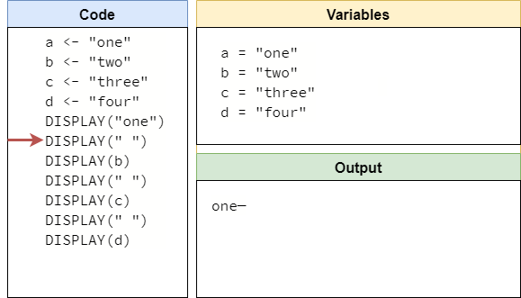
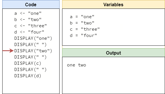
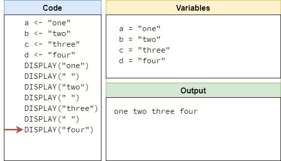
By that definition, each use of the DISPLAY(expression) statement will add a space to the output. So, programs like this:
DISPLAY("one")
DISPLAY("two")
will produce nice, clean output like this:
one twoWe believe this is done to simplify the formatting for answers on the AP exams, which must be hand-written. By automatically including the space in the DISPLAY(expression) statement, it becomes easy to construct a single line of output consisting of multiple parts, and they will be spaced nicely.
However, when trying to print output on multiple lines, the AP CSP Pseudocode does not provide a clear definition for how to accomplish that. For example, adding a newline symbol at the end of the line, like this:
DISPLAY("one\n")
DISPLAY("two")
will result in output with an awkward space at the beginning of the second line:
one
 two
This could be resolved by adding the newline at the beginning of the next line, like so:
DISPLAY("one")
DISPLAY("\ntwo")
However, this is rarely done in real programming languages, since most languages have a display statement that adds a newline at the end by default, and most programmers are used to that convention. Therefore, we don’t feel that it is proper to teach this method, only to adjust later on to fit with a more proper style.
Likewise, there is no way to use a DISPLAY(expression) statement without adding a space at the end, which is something that is very useful in many situations.
Therefore, we’ve chosen to redefine the DISPLAY(expression) statement to not append a space at the end of the line. That aligns it with statements that are available in most common programming languages.
Subsections of Using Display
Pseudocode Variables
YouTube VideoResources
Now that we’ve learned how to use the DISPLAY(expression) statement, let’s focus on the next major concept in pseudocode, as well as any other programming language: variables.
The word variable is traditionally defined as a value that can change. We’ve seen variables like $x$ used in Algebraic equations like $x + 4 = 7$ to represent unknown values that we can try to work out. In programming a variable is defined as a way to store a value in a computer’s memory so we can retrieve it later. One common way to think of variables is like a box in the real world. We can put something in the box, representing our value. Likewise, we can write a name on the side of the box, corresponding to our variable’s name. When we want to use the variable, we can get the value that it currently stores, and even change it to a different value. It’s a pretty handy mental metaphor to keep in mind!
Creating Variables
To use a variable, we must first create one. In pseudocode, we create a variable in a special type of statement called an assignment statement. The basic structure for an assignment statement is a <- expression. When our “mental model” runs this statement, it will first evaluate expression into a single value. Then, it will store that same value (we can think of this as a copy of that value) in the variable named a. For example, the statement:
x <- "Hello World"will store the string value “Hello World” into a new variable named x. Pretty handy!
Now, let’s cover some important rules related to assignment statements:
- Assignment statements are always written with the variable on the left, and an expression on the right. We cannot reverse the statement and say
expression -> xin programming like we can in math. In mathematical terms, this means an assignment statement is not commutative. - The left side of an assignment statement must be a location where a value can be stored. For now, we only have single variables in our pseudocode so that’s all we’ll use, but later on in this course we’ll learn about lists as another way to store data.
- The right side of an assignment statement must be an expression that evaluates to a value that can be stored in the location given on the left side. We’ll spend more time discussing this in future labs, but it is an important rule to know.
Using Variables
Once we’ve created a variable, we can use a variable in an expression to retrieve its current value. For example, we can now rewrite our previous “Hello World” program to use a variable like this:
x <- "Hello World"
DISPLAY(x)
Notice that we don’t put quotes around the variable x in the DISPLAY(expression) statement like we did before. This is because we want to evaluate the variable x and display the value it contains, not display the string "x". Remember that quotes are only placed around string values, but variables are used without quotes around them. So, when we run this program on our “mental model” of a computer, we should get this output:
Hello WorldGreat! We’ve learned how to use variables in our programs.
Updating Variable Values
We can easily update the value stored in a variable by simply using another assignment statement in our code. For example, consider this program that displays two lines of output:
x <- "First line\n"
DISPLAY(x)
x <- "Second line"
DISPLAY(x)
When we run this program, we should see the following output:
First line
Second line
Notice how we are printing the variable x twice in the program, but each time it displayed a different value? This is because the value stored in x can change while the program is running, but when we evaluate it, we only get the value that it is currently storing. This is why we call items like x variables - because their value can change!
note-2
Let’s talk about variable names for a minute. There is an old joke in computer science that says “the two most difficult things in computer science are dealing with cache invalidation and naming things.” We won’t learn about cache invalidation for a while (it’s a pretty advanced topic), but as we spend more time writing code, we’ll probably find out that coming up with good and useful variable names can indeed be difficult. It might even derail your progress for a bit while you try to come up with the most perfect variable name ever.
Most languages have some rules for how variables should be named, and our pseudocode is no different. Likewise, there are some conventions that most programmers follow when naming variables, even though they aren’t required to. Thankfully, these conventions can be bent or broken at times depending on the situation.
In this course, we’ll follow the following rules when it comes to naming variables:
- A variable name must begin with a letter.
- Variable names must only include letters, numbers, and underscores. No other symbols, including spaces, are allowed.
Beyond that, here are a few conventions that you should follow when naming your variables:
- Variables should have a descriptive name, like
totaloraverage, that makes it clear what the variable is used for. - Variables should be named using Snake Case
. This means that spaces are represented by underscores
_, as innumber_of_inputs - Try to use traditional variable names only for their specific uses. Some examples of traditional variable names:
tmportempare temporary variables.i,j, andkare iterator variables (we’ll learn about those later).x,y, andzare coordinates in a coordinate plane.r,g,b,aare colors in an RGB color system.
- Variables should not have the same name as keywords or any built-in statements or expressions in the language.
- For example, our pseudocode has a
DISPLAY()statement, so we should not name a variableDISPLAYin our language.
- For example, our pseudocode has a
- In general, longer variable names are more useful than short ones, even if they are more difficult to type.
That said, in many of the code reading and writing examples in this course, you’ll see lots of simple variable names that are not descriptive at all. This is because the point of the exercise is to read and understand the code itself, not simply inferring what it does based on the variable names. We’ll still follow the rules, but we may ignore some or all of the conventions in our code.
Subsections of Pseudocode Variables
Variables
YouTube VideoResources
The print(expression) statement is very powerful in Python, but we really can’t do much with our programs using just a single statement. So, let’s look at how we can use variables in Python as well.
Recall that a variable is a value that can change. In programming, it is easiest to think of a variable as a place in memory where we can store a value, and then we can recall it later by using that variable in an expression. In a later lab, we’ll learn how to use operators to manipulate the values stored in variables, but for right now we’re just going to focus on storing and retrieving data using variables.
Creating Variables
The process for creating a variable in Python is very similar to what we observed in pseudocode. Once again, we’re going to use an assignment statement to create a variable by storing a value in that variable. An assignment statement in Python looks like a = expression, where a is the name of a variable, and expression is an expression that evaluates to a value that we can store in that variable. For example, let’s consider the Python statement:
x = "Hello World"In that statement, we are storing the string value "Hello World" in the variable named x. It’s just like we expect it to work based on what we’ve already learned in pseudocode.
Let’s review some of the important rules about variables that we’ve learned so far:
- Assignment statements are always written with the variable on the left, and an expression on the right. This is a bit more confusing in Python, since we are used to the equals
=symbol being commutative in math, meaning that we can swap the left and right side and it will still be a true statement. However, in Python, the equals=symbol is only used for assignment statements, and it must always have the variable on the left and an expression on the right. - The left side of an assignment statement must be a location where a value can be stored. Once again, we’re just going to work with single variables, so we don’t have to worry about this yet. In a later lab, we’ll introduce lists as another way to store data, and we’ll revisit this rule.
- The right side of an assignment statement must be an expression that evaluates to a value that can be stored in the location given on the left side. Similar to the rule above, right now we’re only working with string values, so we don’t have to worry about this rule yet. We’ll come back to it in a future lab.
Using Variables
Once we’ve created a variable, we can use it in any expression to recall the current value stored in the variable. So, we can extend our previous example to store a value in a variable, and then use the print(expression) statement to display it’s value. Here’s what that would look like in Python:
x = "Hello World"
print(x)
Just like in pseudocode, notice that we don’t put quotation marks " around the variable x in the print(expression) statement. This is because we want to display the value stored in the variable x, not the string value "x". So, when we run this code, we should get this output:
Hello WorldTo confirm, feel free to try it yourself! Copy the code above into a Python file, then use the python3 command in the terminal to run the file and see what it does. Running these examples is a great way to learn how a computer actually executes code, and it helps to confirm that your “mental model” of a computer matches how a real computer operates.
Updating Variable Values
Python also allows us to change the value stored in a variable using another assignment statement. For example, we can write some Python code that uses the same variable to print multiple outputs:
a = "Output 1"
print(a)
a = "Output 2"
print(a)
When we run this code, we’ll see the following output:
Output 1
Ouptut 2
So, just like we observed in pseudocode, when we evaluate a variable in code, it will result in the value currently stored in that variable at the time it is evaluated. So, even though we are printing the same variable twice, each time it is storing a different value. Recall that this is why we call items like a a variable - their value can change!
Variable Names
Finally, Python uses many of the same rules for variable names that we introduced in pseudocode. Let’s quickly review those rules, as well as some conventions that most Python developers follow when naming variables.
First, the rules that must be followed:
- Variable names must begin with either a letter or an underscore
_. - Variable names may only contain letters, numbers, and underscores
-. - Variable names are case sensitive.
Next, here are the conventions that Python developers follow for variable names, which we will also follow in this course:
- Variable names beginning with an underscore
_have a special meaning. So, we won’t create any variables beginning with an underscore right now, but later we’ll learn about what they mean and start using them. - Variables should have a descriptive name, like total or average, that makes it clear what the variable is used for.
- Variables should be named using Snake Case
. This means that spaces are represented by underscores
_, as innumber_of_inputs - Try to use traditional variable names only for their specific uses. Some examples of traditional variable names:
tmportempare temporary variables.i,j, andkare iterator variables (we’ll learn about those later).x,y, andzare coordinates in a coordinate plane.r,g,b,aare colors in an RGB color system.
- Variables should not have the same name as keywords or any built-in statements or expressions in the language.
- For example, Python has a
printstatement, so we should not name a variableprintin our language.
- For example, Python has a
- In general, longer variable names are more useful than short ones, even if they are more difficult to type.
Finally, don’t forget that some of the code examples in this course will not follow these conventions, mainly because long, descriptive variable names might give away the purpose of the code itself. We’ll still follow the rules that are required, but in many cases we’ll use simple variable names so that the focus is learning to read the structure of the code, not inferring what it does based solely on the names of the variables.
Subsections of Variables
Code Tracing
YouTube VideoResources
As our programs become more complex, it can become more and more difficult to run them on our “mental model” of a computer without a little bit of help. So, let’s go through an example of code tracing, one of the best ways to work through large blocks of code and keep track of everything that is going on. At the same time, we can also learn more about using variables in our programs!
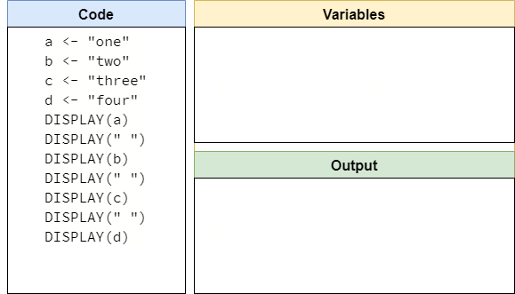
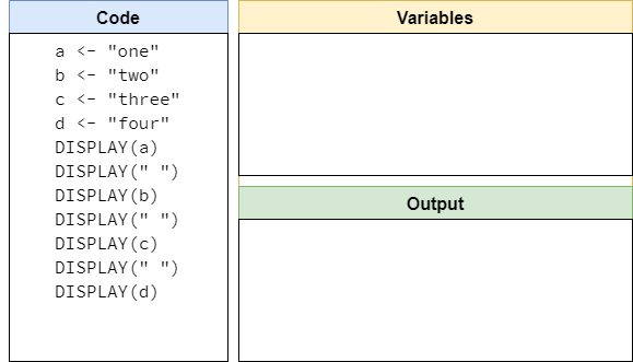
Multiple Variables
Our programs can also have multiple variables. In fact, there is no limit to the number of variables we can use - it just requires us to come up with a unique name for each one. For example, we could make a program that includes and displays multiple variables like this:
a <- "one"
b <- "two"
c <- "three"
d <- "four"
DISPLAY(a)
DISPLAY(" ")
DISPLAY(b)
DISPLAY(" ")
DISPLAY(c)
DISPLAY(" ")
DISPLAY(d)
This is a pretty complex program - one of the most difficult we’ve seen so far! To work out what it does, we can use a technique called code tracing. Let’s see how it works!
Code Tracing
Code tracing involves mentally walking through the code line by line and recording what each line does. So, we’ll need to keep track of the current values of each variable, as well as the current output that is displayed to the user. We can easily do this by making a couple of boxes on a sheet of paper or in a couple of tabs of a text editor. For this example, we’ll use a simple graphic like this one:
As we run the program, we’ll keep track of which line of code we are on, and update the trace as we go. So, let’s start by running the first line of code, a <- "one". When we run this line, we’ll need to create a new variable named a and store the value "one" in it. In our code trace, we can simply add an entry to the variables section as shown below:
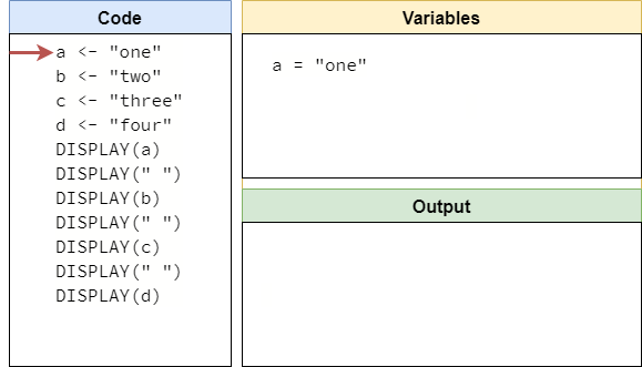
There is no right or wrong way to record variables in our code trace. We can use boxes for each value and update it as we go, or just write a short text entry as shown in our example. Any method is valid. In the meantime, we’re using an arrow to keep track of which line we are running in our program, but we can just as easily do so with a finger or other tool in the real world!
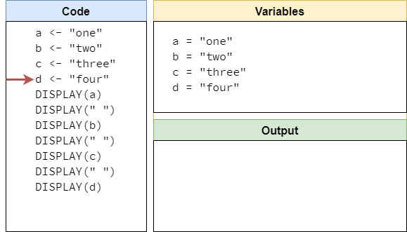
Looking at the next three lines of code, we see that they are all similar. So, we can quickly run them and populate the next four entries in our variables box:
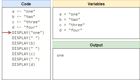
Now we’ve reached the first DISPLAY(expression) statement in our program. If we recall the way those statements work, we should first evaluate the expression into a value. In our code, our expression is the variable a, which isn’t a value. So, we need to evaluate it by looking up the current value of a and placing it in the current line of code. Then, we can display that value in the output. So, once we’ve run that line of code, our code trace will look something like this:
The next line of code is just DISPLAY(" "), which is simple since the expression " " is just a string value that doesn’t need to be evaluated. So, we’ll need to add a space to the end of our output. This can be tricky, since we really can’t “see” spaces. For now, we’ll just place a dash - in that space until we get the next piece of output.
Now we are back to a line that contains a variable. So, once again we look at the current value of the variable, place it in the expression, and then update our output. Since we’ve now received more output, we can remove that dash to make it a bit clearer.
From here on out, it should be pretty simple to figure out how the rest of this trace goes. When we are finished, we should have a code trace that looks like this:
The whole process is shown below in animated form:
Code tracing is a great way to train our “mental model” to work just like a real computer. While this may seem like a slow and tedious process right now, remember all of the other things we’ve learned how to do. Reading is initially very difficult, but with time and practice we can go from recognizing individual letters, to sounding out words, and finally reading with ease! The same happens as we learn to program and read code - with practice we’ll be able to do this in our head quickly and easily!
Subsections of Code Tracing
Variables in Expressions
YouTube VideoResources
Let’s look at one more difficult concept in programming - using variables in the expressions for other variables. Right now we haven’t learned any operators (don’t worry - we’ll cover those in great detail in a future lab), but it is still important for us to understand what happens when we use the value in one variable to create or update the value in another variable.
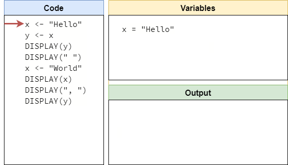
Let’s consider this program:
x <- "Hello"
y <- x
DISPLAY(y)
DISPLAY(" ")
x <- "World"
DISPLAY(x)
DISPLAY(", ")
DISPLAY(y)
To work out what this program displays, we can once again use code tracing to work through it line by line. The first line is pretty easy - we see that we are simply storing the string value "Hello" in a new variable named x, so we can easily update that on our code trace as shown below:
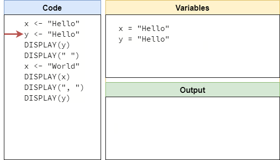
The next line is tricky - here we are storing the expression x into the variable named y. As before, we first have to evaluate the expression x to a value, which is simply the value stored in that variable. So, in actuality, we are storing the string value "Hello" in the variable y as well.
This is important to understand! In the code, and indeed in our “mental model” of a computer, we might start to think that the values stored in variable x and y are connected somehow. However, this is not the case. What the line y <- x says is simply that y now stores a copy of the value that was stored in x when this line is run. Going forward, these two values are not connected in any way, as we’ll soon see.
So, after running the second line of code, our code trace should now look like this:
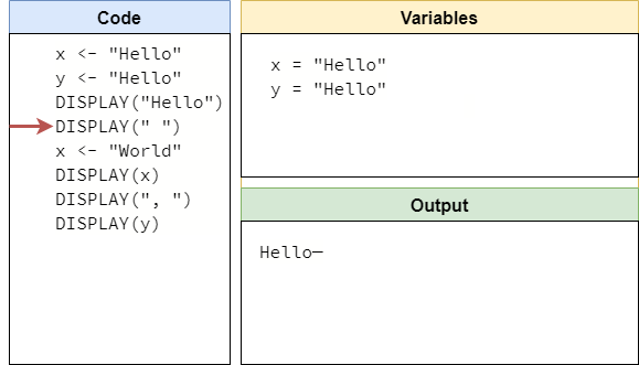
The next two lines are pretty simple, since they only display the value stored in y followed by a space. So, after running those two lines, we should see the following on our code trace:
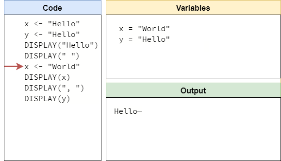
Now we reach the most important line, x <- "World". When we run this line, we’ll update the value stored in x to be the string value "World". However, this will not change the value stored in y. This is because y stores a copy of the value that was previously stored in x, and any changes to the value stored in x will not impact the value stored in y at all. So, after running that line, our code trace should show the following:
Once we’ve done that, running the next three lines of code is pretty straightforward. We’ll just display the current value stored in in x and y, with a comma and space between them. So, at the end, our code trace should look like this:
The entire trace can be seen in the animation below:
As we have learned, code tracing is a very important skill, and it helped us discover one of the most important rules about working with variables: when we assign the value of one variable into another, we copy the existing value, but those two variables are not related to each other after the fact.
Subsections of Variables in Expressions
Python Introduction
YouTube VideoIn this lab, we’re going to take what we’ve learned in pseudocode and see how it transfers to a real programming language, Python. We’ve chosen Python because it is very easy to learn, easy to use, and it is used in many different places, from scientific computing and data analysis to web servers and even artificial intelligence. It is a very useful language to learn, and it makes a great first programming language.
We’ve already built a pretty effective “mental model” of a computer by working in pseudocode. So, as we work through this lab, we’ll need to constantly pay attention to how a real computer works, and make sure that our “mental model” is accurate. If not, we’ll have to adapt our understanding of a computer to match the real world. This process of adaptation and accommodation is an important part of learning to program - we have to have a good understanding of what a computer actually does when it runs our code, or else we won’t be able to write code that will do what we want it to do.
As we learn to write code in a real programming language, it helps to refer to the actual documentation from time to time. So, we recommend bookmarking the official Python Documentation as a great place to start. Throughout this course, we may also include links to additional resources, and those are also worth bookmarking. One of the best parts about programming is that nearly all of the documentation is online and easily accessible, and learning how to quickly search for a particular solution or reference is just as useful as knowing how to do it from memory. In fact, most programmers really only know the basics of the language and a few handy tricks, and the rest of it is just reading documentation and learning when to use it. So, don’t worry about remembering it all right from the start - instead, learn to read the documentation and use the tools that are available, and focus on understanding the basics of the language’s syntax and rules.
Subsections of Python Introduction
Working in the Terminal
YouTube VideoResources
First, let’s start with the basics of writing Python code in a file and running those files. This is the first major step toward actually writing a real program, but it can definitely be difficult the first time without prior experience to rely on. So, let’s go through it step by step and make sure we know how to run our programs in Python.
At this point, we should already have Python installed on our system. For students using Codio, this is taken care of already. For students using their own computers, refer to an earlier lab to find instructions for installing Python on your system, or contact the instructors for assistance.
To make sure that Python is installed and working, we’ll need to open a terminal in our operating system. In Codio, this can be found by clicking the Tools menu at the top, and then choosing Terminal. More information can be found in the Codio Documentation . There may also already be one open for you if you are reading this content from within Codio.
If you are working on your own computer, you’ll need to open a terminal on your operating system. This should have been covered in the previous lab when you installed Python. On Windows, look for Windows Terminal or Windows PowerShell (not the old Command Prompt, which requires different commands). On Mac or Linux, look for an application called Terminal. Throughout this course, we’ll call these windows the terminal, even though they may have slightly different names in each operating system.
Once we have the terminal open, we should see something like one of these examples:


At this point, we should see a place with a blinking cursor, where we can type our commands. This is called the command prompt in the terminal. The first thing we can do is check to make sure Python is properly installed, and we can also confirm that it is the correct version. To do this, we’ll enter the following command and press enter to execute it:
python3 --versionHopefully, that command should produce some output that looks like this:
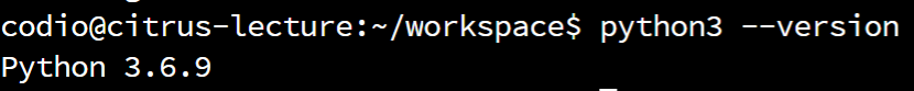
Here, we see that the currently installed Python version is 3.6.9. As long as your Python version number begins with a 3, you have correctly installed Python and are able to run it from the terminal. So, we can continue to the next part of this lab.
If you aren’t able to run Python or aren’t sure that you have the correct version, contact the instructor for assistance!
note-1
Notice that we have to use the command python3, including the version number, instead of the simpler python command here. This is because some systems may also have Python version 2, an outdated version of Python, installed alongside version 3. In that case, the simple python command will be Python version 2, while python3 will be Python version 3. Unfortunately, most programs written in Python 3 will not run properly in Python 2, so it is important for us to make sure we are using the correct Python version when running our programs.
Thankfully, the command python3 should always be Python version 3, and using that command is a good habit to learn. However, depending on how Python is installed on Windows, it might only work via the python command, which can make it confusing. So, throughout this course, we will use the command python3 to run Python programs, but you may have to adapt to your particular situation.
Navigating in the Terminal
When we open a terminal, it will usually start in our user’s home folder. This may mean different locations for different operating systems. For example, if our current user’s name is <username>, the terminal will usually start in this location for each operating system:
- Windows:
C:\Users\<username> - Linux:
/home/<username> - Mac:
/Users/<username> - Codio:
/home/codio/workspace
The directory that is open in the terminal is known as the working directory. We can use the pwd command to determine what our current directory is:
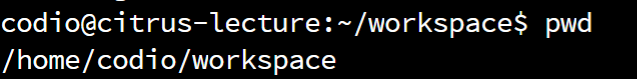
In this example, we are looking at the Codio terminal, so our working directory is /home/codio/workspace.
Next, we can see the files and directories contained in that directory using the ls command. Here’s the output of running this command in Codio:
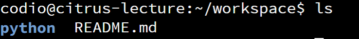
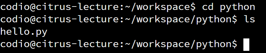
In the output, we can see that there is a file named README.txt and a directory named python. In Codio, we’ll place all of our files in the python directory, so we can open that using the cd python command:
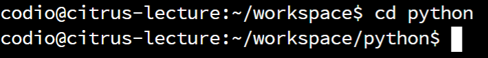
Notice how the python directory is now included in the command prompt in the terminal. Most terminals will show the working directory in the command prompt in some way.
That’s the basics of navigating in the terminal, but there is much more to learn. If you’d like to know more, consider checking out some of the resources linked below!
Resources
- Basic Linux Navigation & File Management from DigitalOcean
- Beginner’s Guide to the Bash Terminal by Joe Collins on YouTube
note-2
Most of the content in this course will focus on using the commands that are present in the Linux terminal, since they are the most widely-used commands across all platforms. In general, these commands should work well on both Windows and Mac, with a few caveats:
- On Windows, there is an older Command Prompt tool that does not support the newer Linux commands. Therefore, we won’t be using it. Instead, we only want to use Windows PowerShell, which supports most of the basic Linux commands via aliases to similar PowerShell commands. We can also install the Windows Terminal application for a more modern interface.
- Windows users may also choose to install the Windows Subsystem for Linux (WSL) to run Linux (such as Ubuntu) directly within Windows. Many developers choose to pursue this option, as it provides a clean and easy to use development environment that is compatible with the Linux operating system.
- The Mac operating system includes a terminal that uses either ZSH (since OS X 10.15) or Bash (OS X 10.14 and below). This terminal is very similar to the Linux terminal when it comes to navigating the file system and executing programs, which is sufficient for this course.
Fully learning how to use these tools is outside of the scope of this class, but we need to know enough to navigate the filesystem and execute the python3 command. If you need assistance getting started with this step, your best bet is to contact the instructors. Each student’s computer is a bit different, so it is difficult to cover all possible cases here.
Subsections of Working in the Terminal
Print Statement
YouTube VideoResources
The first statement that we’ll cover in the Python programming language is the print(expression) statement. This statement is used to display output to the user via the terminal. So, when Python runs this statement, it will evaluate the expression to a single value, and then print that value to the terminal.
For example, the simplest Python code would be a simple Hello World program, where we use the print(expression) statement to display the text "Hello World" to the user:
print("Hello World")When we run that program in Python, we’ll see the following output:
Hello WorldJust like in pseudocode, strings in Python are surrounded by double-quotes ". For now, we’re just going to work with string values, but in a later lab we’ll introduce numerical values and discuss how to use them as well.
Let’s go through the full process of writing and running that program in Python!
Writing a Python Program
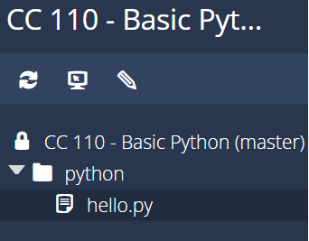
The first step to create a program in Python is to create a text file to store the code. This file should have the file extension .py to indicate that it is a Python program. So, we’ll need to create that file either on our computers or in Codio or another tool if we are using one. For example, in Codio we can create the file in the python folder by right-clicking on it and selecting the New File option. We’ll name the file hello.py:
Once we’ve created that file, we can then open it by clicking on it. In Codio and in other online tools, it will open in the built-in editor. On a computer, we’ll need to open it in a text editor specifically designed for programming. We recommend either Atom or Visual Studio Code , which are available on all platforms. Tools like the built-in Notepad tool on Windows, or a word processor like Word or Pages do not work for this task.
In that file, we’ll simply place the code shown above, like this:
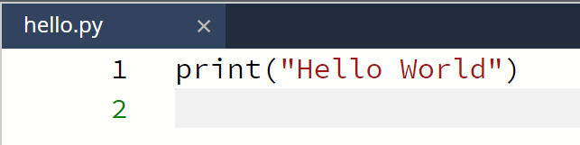
That’s all there is to it!
Running a Python Program
Once we’ve written the code, we can open the Terminal and navigate to where the code is stored in order to run the program. On Codio, we’ll just use the cd python command to enter the python directory. On a computer, we’ll need to navigate the file system to find the location where we placed our code. We highly recommend creating a folder directly within the home directory and placing all of our code there - that will make it easy to find!
Once we are in the correct directory, we can use the ls command to see the contents of that directory. If we see our hello.py file, we are in the correct location:
If we don’t see our file, we should make sure we’ve saved it and that our current working directory is the same location as where the file is stored.
Finally, we can execute the file in Python using the python3 command, followed by the name of the file:
python3 hello.pyIf everything works correctly, we should see output similar to this:
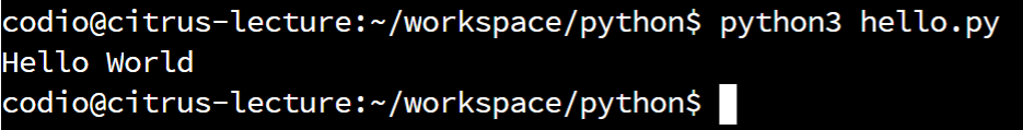
There we go! We’ve just run our first program in Python! That’s a great first step to take.
Of course, there are lots of ways that this could go wrong. So, if you run into any issues getting this to work, please take the time to contact an instructor and ask for assistance. This process can be daunting the first time, since there are so many things to learn and so many intricacies we simply don’t have time to cover up front. Don’t be afraid to ask for help!
Subsections of Print Statement
Using Print
YouTube VideoResources
The print(expression) statement in Python works in much the same way as the DISPLAY(expression) statement in pseudocode, but with one major difference. In pseudocode, the DISPLAY(expression) statement will print the value from the expression to the user, but it won’t add anything like a space or newline to the end. In Python, however, the print(expression) statement will add a newline to the end of the output by default. This means that multiple print(expression) statements will print on multiple lines. Let’s look at some examples!
Throughout this course, we’ll show many different code examples and their output here in the lab. To test them out, feel free to copy the code examples to a Python file and run it yourself. You can even tweak them to do something new and see how Python interprets different pieces of code. In the end, the best way to learn programming is to explore, and running these examples on your own is a great way to get started!
Multiple Lines
In Python, we can print multiple lines of output simply by using multiple print(expression) statements:
print("a")
print("b")
print("c")
print("d")
will result in this output:
a
b
c
d
We can also include a newline symbol \n in a print(expression) statement in Python. This will add a newline to the output, and then the print(expression) statement will add an additional newline at the end of the value that is printed:
print("one\ntwo")
print("three\nfour")
will produce this output:
one
two
three
four
Printing On the Same Line
What if we want to display multiple print(expression) statements on the same line? To do that, we must add an additional option to the print(expression) statement - the end option.
For example, the following code will produce output all on the same line:
print("Hello ", end="")
print("World!")
In this example, we set end to be an empty string "". When we run this program, we’ll get the following output:
Hello World!In fact, in Python, the print(expression) statement is an example of a function in Python. Functions in Python are like procedures in pseudocode - when we call them, we write the name of the function, followed by a set of parentheses and then arguments separated by commas within the parentheses. So, in actuality, the expression in the print(expression) statement is just the first argument when we call the print function.
Therefore, the end option that we showed above is just a second argument that is optional - it simply let’s us choose what to put at the end of the output. By default, the end parameter is set to the newline symbol \n, so if we don’t provide an argument for end it will just add a newline at the end of the value.
We can set the value of end to be any string. If we want to include a space at the end of the output, we can add end=" " to the print function call.
In this course, we won’t spend much time talking about optional parameters and default values in Python functions, but it is important to understand that statements like print are actually just Python functions behind the scenes!
Subsections of Using Print
Python Tutor
YouTube VideoResources
As we learn to write more complex programs in Python, it is important to make sure we can still mentally execute the code we are writing in our “mental model” of a computer before we actually run it on a computer. After all, if we don’t have at least an idea of what the code actually does before we write it, we really haven’t learned much about programming!
Thankfully, when working in a real programming language such as Python, there are many tools to help us visualize how the code works when we run it. This helps us continue to develop our “mental model” of a computer by looking behind the scenes a bit to see what is happening when we run our code.
One such tool is Python Tutor , a website that can quickly run short pieces of Python code to help us visualize what each line does and how it works. This tool is also integrated directly into Codio!
Python Tutor Example
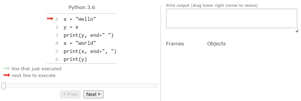
Let’s look at an example of how Python Tutor compares to the manual code traces we performed in a previous lab. For this example, we’re going to use the following code:
x = "Hello"
y = x
print(y, end=" ")
x = "World"
print(x, end=", ")
print(y)
In Codio, we can see the visualization in a tab to the left. It will visualize the content in the tutor.py file in the python directory, so make sure that the contents of the tutor.py file match the example above before continuing.
Outside of Codio, this visualization can be found by clicking this Python Tutor Link to open Python Tutor on the web.
Stepping Through Code
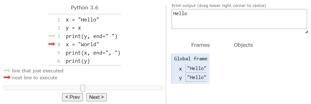
The initial setup for Python Tutor is shown in the image below:

This looks similar to the setup we used when performing code tracing with pseudocode. We have an arrow next to our code that is keeping track of the next line to be executed, and we have areas to the side to record variables and outputs. In Python Tutor, the variables are stored in the Frames section. We’ll learn why that is important later in this lab when we start looking at Python functions.
So, let’s click the Next > button once to execute the first line of code. After we do that, we should see the following setup in Python Tutor:
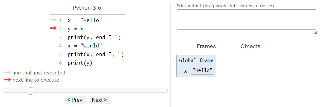
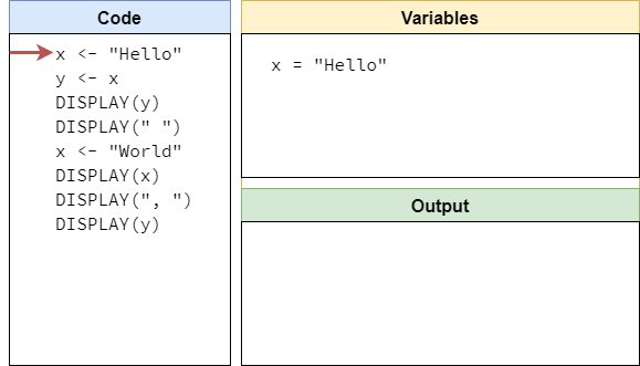
That line is an assignment statement, so Pyhton Tutor added an entry in the Frames section for the variable x, showing that it now contains the string value "Hello". It placed that variable in a frame it is calling the “Global frame,” which simply contains variables that are created outside of a function in Python.
When we click the Next > button again, we should see this:
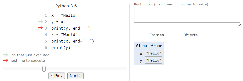
Once again, the line that was just executed is an assignment statement, so Python Tutor will add a new variable entry for y to the list of variables. It will also store the string value "Hello". Just like before, notice that the variable y is storing the same value as x, but it is a copy of that value. The variables are not connected in any other way.
We can click Next > again to execute the next line of code:
Once this line is executed, we’ll see that it prints the value of the variable y to the output. Python Tutor will look up the value of y in the Frames section and print it in the output, but it won’t evaluate the expression in the code like we did when we performed code tracing in pseudocode. It’s a subtle difference, but it is worth noting.
Once again, we can click Next > to execute the next assingment statement:
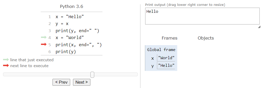
This statement will update the value stored in the variable x to be the string value "World". After that, we can run the next statement:
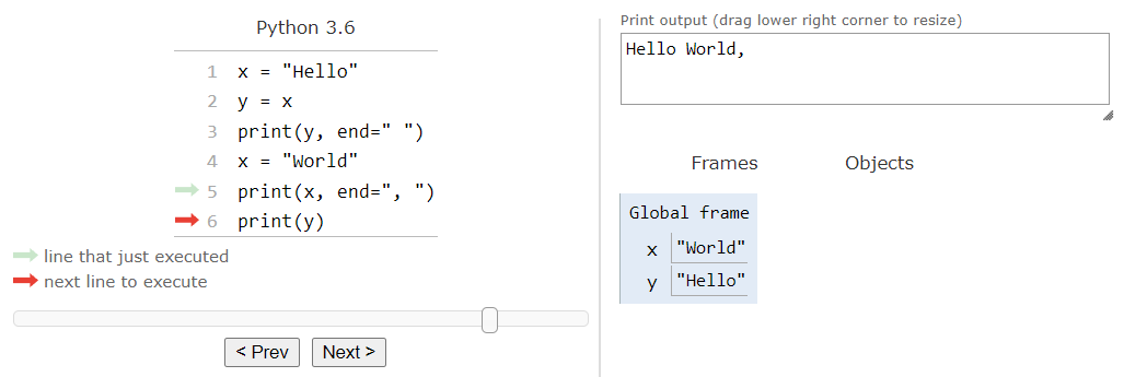
That statement prints the value of x to the output, followed by a comma , and a space as shown in the end argument provided to the print function. Finally, we can click Next > one more time to execute the last line of code:
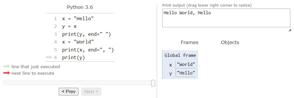
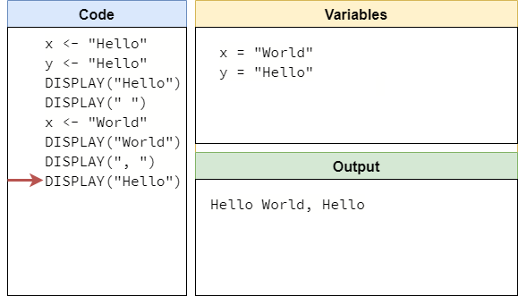
This will print the value of y to the output. Once the entire program has been executed, we should see the output Hello World, Hello printed to the screen.
The full process is shown in the animation below:
Using tools like Python Tutor to step through small pieces of code and understand how the computer interprets them is a very helpful way to make sure our “mental model” of a computer accurately reflects what is going on behind the scenes when we run a piece of Python code on a real computer. So, as we continue to show and discuss examples in this course, feel free to use tools such as Python Tutor, as well as just running the code yourself, as a great way to make sure you understand what the code is actually doing.
Subsections of Python Tutor
Summary
Pseudocode
In this lab, we introduced a simple pseudocode programming language, based on the one used by the AP Computer Science Principles exam. This pseudocode language includes several statements and rules we’ve learned to use in this lab. Let’s quickly review them!
Display Statement
The DISPLAY(expression) statement is used to display output to the user.
- It will evaluate
expressionto a value, then display it to the screen. - It does not add any additional spaces or newlines after the value is displayed
- We can display spaces using
DISPLAY(" "), and we can use the newline symbol to go to the next lineDISPLAY("\n")
Assignment Statement
The assignment statement, like a <- expression is used to create variables and store values in the variables.
- The variable must be on the left side, and the right side must be an expression that evaluates to a single value.
- If the variable does not exist, it is created. Otherwise, the current value of the variable is replaced by the new value.
- Variable names must begin with a letter, and may only contain letters, numbers, and underscores.
Summary
This pseudocode language may seem very simple, but we’ve already learned a great deal about how programming works and how a computer interprets a program’s code, just by practicing with this very simple language. In the next lab, we’ll see how these concepts directly relate to a real programming language, Python. For now, feel free to keep practicing by writing programs and pseudocode and running them on your “mental model” of a computer. It is a very important skill to develop!
Python
We also introduced some basic statements and structures in the Python programming language. Let’s quickly review them!
Print Statement
The print(expression) statement is used to print output on the terminal.
- It will evaluate
expressionto a value, then display it to the screen. - By default, it will add a newline to the end of the output.
- We can change that using the
endparameter, such asprint(expression, end="")to remove the newline.
Assignment Statement
The assignment statement, like a = expression is used to create variables and store values in the variables.
- The variable must be on the left side, and the right side must be an expression that evaluates to a single value.
- If the variable does not exist, it is created. Otherwise, the current value of the variable is replaced by the new value.
- Variable names must begin with a letter or underscore, and may only contain letters, numbers, and underscores.
- Variable names beginning with an underscore have a special meaning, so we won’t use them right now.
Summary
As we’ve seen, the Python language is very similar to the pseudocode language we’ve already learned about. Hopefully the practice we have in reading and writing pseudocode using our “mental model” of a computer will help make it even easier to read and write Python code that is meant to be run on an actual computer.