Chapter X
CIS 115 Labs
This section contains the content for CIS 115’s Prelabs.
This section contains the content for CIS 115’s Prelabs.
In this lab, we’re going to cover various ways to install Python on your computer. First, we’ll cover the basic way to install Python on a Windows system. To begin, open a web browser and go to python.org/downloads. Here you can find downloads for the latest version of Python for Windows as well as other operating systems. I’m going to click the button here to download the latest version of Python for Windows.
Once the file is downloaded, I can double click it to open and run the installer. When we run the installer, there are a couple of options that we’ll want to change. Notice by default, it will install Python into this complicated directory here, which can make it very hard to find. Also, it does not add Python to the path which we definitely want to do. So we’ll check mark this checkbox and then we will customize the installation. We’ll go ahead and check mark the boxes to install all of the optional features. When choosing advanced options, we can check mark the option to install for all users, which will place Python in the program files directory, making it much easier to find. We can click install and it will install very quickly.
Once we’ve installed Python on our computer, we can verify that it works by loading it in PowerShell. On Windows, I’m just going to search for PowerShell in the start menu to find that program. Once PowerShell loads, we can run Python using the python command. Notice that this is different than most Linux and Mac systems where to run Python version three, we must run the command python3. On Windows with the most recent installer, we can simply use the python command followed by --version to see the current version of Python. If we type python3, it might load the Microsoft Store in prompting us to install an older version of Python. This can get a bit confusing, it’s one of the problems with Python is the inconsistent usage of the python command to refer to Python version two, and Python version three. So if you follow this guide to install Python on your computer, just be aware that anytime you see the python3 command in documentation or in the labs, you’ll just need to use the python command instead, which will run Python version three.
To make it easy to write Python files on Windows, you may also want to install a text editor that is specifically designed for writing code. One of the easiest to use is Atom which is a text editor provided from GitHub. So we’ll download and install that as well. Once again, once we’ve downloaded Atom, we can double click the installer to install it. Once Atom is installed and open, you can close all of the open tabs to get a view that looks like this.
To make it easy to program in Python, we’re going to create a folder just for the Python work in this course. To do that, I’m going to click the add folders button right here. In Windows, we recommend creating a folder inside of your users home directory for all of your programming work. By default, it will open up the Documents List. But to get to your users folder, we’re going to go to the C drive, then Users. Then we’ll find our username. And then in here, we’re going to create a new folder. And I’m going to name this cis115 to match the class. And we’ll select that folder as the folder to open in Atom. Now we see a view similar to this.
From here, we can easily add a Python file by right clicking on the folder and creating a new file. I’m going to name this file hello.py. And then inside of that file, I can type print hello world as a simple Hello World program. Once I’ve written that program, I can go to the File menu and choose to save the file. I can also use Ctrl+S to Save the file. Once I’ve done that that file should now exist on my system in that folder.
Once we’ve done this, we can run this file using Python by again opening PowerShell. In PowerShell, we need to navigate to where that is that folder is found. Notice that PowerShell already opens into our users folder. So all we should have to do is type cd cis115 to open up that folder. Then we can type python and the name of the file that we just created to run it. There we go. That’s all it takes to run a Python program on your Windows system. It should give you enough to get started in this class. As always if you have any questions please feel free to reach out to either of the instructors or any of our TAs and we’d be happy to assist you
Learning to program involves learning not only the syntax and rules of a new language, but also a new way of thinking. Not only do we want to write code that is understandable by the computer, we must also understand what the computer will do when it tries to run that code.
A key part of that is learning to think like a computer thinks. We sometimes call this our “mental model” of a computer. If we have a good “mental model” of a computer, then we can learn to read code and mentally predict what it will do, even without ever running it on an actual computer. This ability is crucial for programmers to develop.
One easy way to develop this ability is to learn how to use a programming language that isn’t an actual programming language. This language cannot (or at least wasn’t intended to) be run on a computer. Instead, we must simply learn to use our “mental model” of a computer to determine what programs written in this language will do.
These languages are sometimes referred to as pseudocode. If we look at the word pseudocode, we see the prefix pseudo, which means “not genuine.” That definition makes sense - a pseudocode is, in essence, not a genuine computer code. So, a pseudocode is simply a programming language that looks like a real programming language, but it isn’t actually intended to be run by a computer.
There are many examples of pseudocode that we could learn. In this course, we’re going to use the pseudocode that is used by the AP Computer Science Principles exam. This is an extraordinarily easy to understand pseudocode, and it covers all of the operations we need to learn in this course. If you want to learn more, you can find the CSP Reference Sheet online by clicking the link.
Throughout this course, we’ll introduce new programming concepts using pseudocode first, which will allow us to learn how they work by adapting our “mental model” of a computer to include the new functionality. By learning how these concepts work in theory first, we’ll be much better able to get them to work in practice on a real computer using Python later. It may sound strange, but this is actually a great way to learn how to program!
In this first lab, we’re going to learn the basics of programming in pseudocode, including how to display message to the user, store information in variables, and write repeatable procedures that we can use as building blocks of a larger program. Let’s get started!
First, let’s start by introducing some important vocabulary terms:
"" in our code and elsewhere.Now that we have learned a few of the important terms used in programming, we can start to discuss the various statements in pseudocode.
In our basic pseudocode, the first and most basic statement to learn is the DISPLAY(expression) statement. This statement will evaluate the expression to a single value, and then it will display that value to the user. In our “mental model” of a computer, this means that the value is printed on the user interface somewhere. The word DISPLAY is an example of a keyword in pseudocode, since it has a special meaning as part of the DISPLAY(expression) statement.
For example, the simplest program we can write is the classic “Hello World” program, which simply displays the message "Hello World" to the user. In pseudocode, that program would look like this:
DISPLAY("Hello World")Notice that the expression part of the statement contains "Hello World" in quotation marks? That is because "Hello World" is text, so we should put it in quotes and make it into a string in our code. Also, since the string "Hello World" can be treated like a value, we can also say it is an expression, and therefore we can use it in the expression part of the statement. This may seem pretty straightforward now, but as our programs become more complex it is important to think about what pieces of code can be treated as values, expressions, and statements.
So, in our “mental model” of a computer, pretend we are using a blank box as our user interface. It might look something like this:
Now, we can run our “Hello World” program in our “mental model” and see what it does. After we run that program, our user interface will now look like this:
Hello WorldAwesome! We’ve just run our first imaginary program! If you look at the output, you might notice something strange - the text on our user interface doesn’t include the quotation marks "" that the expression "Hello World" contained. When we display text to the user, we’ll remove the quotation marks from the beginning and the end of the string, and just display the text inside. Pretty handy!
Each time we run our program, we’ll assume we are starting with an empty user interface. This makes it easy for us to make sure any programs we’ve previously run on our “mental model” won’t interfere with the output of the current program. So, anytime we run the “Hello World” program, even if we run it multiple times back-to-back, our user interface will always look like this:
Hello WorldSo, now that we have that part down, let’s look at creating some more complex programs using this DISPLAY(expression) statement.
Now that we’ve been introduced to the DISPLAY(expression) statement, let’s write a few simple programs using that statement to see how it works. Again, we’re just learning how to run these programs using our “mental model” of a computer, so it is really important for us to closely pay attention to both the code and the output of these examples. We have to learn what rules govern how our computer should work, and the only way to do that is to explore lots of different programs and see what they do.
First, let’s write a simple program that prints 4 letters separated by spaces:
DISPLAY("a b c d")Just like our “Hello World” program, when we run this program, we’ll see that string printed in the user interface:
a b c dOk, that makes sense based on what we’ve previously seen. The DISPLAY(expression) statement will simply display any string expression in our user interface.
Of course, programs can consist of multiple statements or lines of code. So, what if we write a program that contains multiple DISPLAY(expression) statements, like this one:
DISPLAY("one")
DISPLAY("two")
DISPLAY("three")
DISPLAY("four")
What do you think will happen when we try to execute this program on our “mental model?” Have we learned a rule that tells us what should happen yet? Recall on the previous page we learned that it will print the value on the user interface, but that’s it. So, when we execute this program, we’ll see the following output:
onetwothreefourThat’s a very interesting result! We might expect that four lines of code would produce four lines of output, but in fact they are all printed on the same line! This is very helpful, since we can use this to construct more complex sentences of output by using multiple DISPLAY(expression) statements.
If we want to add spaces between each line, we’ll need to include that in our expressions somehow. For example, we could rewrite the program like this:
DISPLAY("one ")
DISPLAY("two ")
DISPLAY("three ")
DISPLAY("four")
Notice that there is now a space inside of the quotation marks on the first three statements? That will result in this output:
one two three fourThere are many other ways we could accomplish this, but this is probably the simplest to learn.
What if we want to print output on multiple lines? How can we do that? In this case, we need to introduce a special symbol, the newline symbol. In our pseudocode, as in most programming languages, the newline symbol is represented by a backslash followed by the letter “n”, like \n, in a string. When our user interface sees a newline symbol, it will move to the next line before printing the rest of the string. The newline symbol itself won’t appear in our output.
For example, we can update our previous program to contain newline symbols between each letter:
DISPLAY("a\nb\nc\nd")This might be a bit difficult to read at first, but as we become more and more familiar with reading code, we’ll start to see special symbols like the newline symbol just like any other letter. For now, we’ll just have to read closely and make sure we are on the lookout for special symbols in our text.
When we run this program in our “mental model” of a computer, we should see the following output on our user interface:
a
b
c
d
There we go! We’ve now figured out how to print text on multiple lines.
We can even extend this to multiple statements! For example, we can update another one of our previous programs to print each statement on a new line by simply adding a newline character to the end of each string:
DISPLAY("one\n")
DISPLAY("two\n")
DISPLAY("three\n")
DISPLAY("four")
When we execute this program, we’ll get the following output:
one
two
three
four
That’s pretty much all we need to know in order to use the DISPLAY(expression) statement to do all sorts of things in our programs!
In this course, we have already introduced one big difference between the AP CSP Pseudocode and our own pseudocode language. In the official CSP Exam Reference Sheet
, the DISPLAY(expression) statement is explained as follows:
Displays the value of
expression, followed by a space.
By that definition, each use of the DISPLAY(expression) statement will add a space to the output. So, programs like this:
DISPLAY("one")
DISPLAY("two")
will produce nice, clean output like this:
one twoWe believe this is done to simplify the formatting for answers on the AP exams, which must be hand-written. By automatically including the space in the DISPLAY(expression) statement, it becomes easy to construct a single line of output consisting of multiple parts, and they will be spaced nicely.
However, when trying to print output on multiple lines, the AP CSP Pseudocode does not provide a clear definition for how to accomplish that. For example, adding a newline symbol at the end of the line, like this:
DISPLAY("one\n")
DISPLAY("two")
will result in output with an awkward space at the beginning of the second line:
one
 two
This could be resolved by adding the newline at the beginning of the next line, like so:
DISPLAY("one")
DISPLAY("\ntwo")
However, this is rarely done in real programming languages, since most languages have a display statement that adds a newline at the end by default, and most programmers are used to that convention. Therefore, we don’t feel that it is proper to teach this method, only to adjust later on to fit with a more proper style.
Likewise, there is no way to use a DISPLAY(expression) statement without adding a space at the end, which is something that is very useful in many situations.
Therefore, we’ve chosen to redefine the DISPLAY(expression) statement to not append a space at the end of the line. That aligns it with statements that are available in most common programming languages.
Now that we’ve learned how to use the DISPLAY(expression) statement, let’s focus on the next major concept in pseudocode, as well as any other programming language: variables.
The word variable is traditionally defined as a value that can change. We’ve seen variables like $x$ used in Algebraic equations like $x + 4 = 7$ to represent unknown values that we can try to work out. In programming a variable is defined as a way to store a value in a computer’s memory so we can retrieve it later. One common way to think of variables is like a box in the real world. We can put something in the box, representing our value. Likewise, we can write a name on the side of the box, corresponding to our variable’s name. When we want to use the variable, we can get the value that it currently stores, and even change it to a different value. It’s a pretty handy mental metaphor to keep in mind!
To use a variable, we must first create one. In pseudocode, we create a variable in a special type of statement called an assignment statement. The basic structure for an assignment statement is a <- expression. When our “mental model” runs this statement, it will first evaluate expression into a single value. Then, it will store that same value (we can think of this as a copy of that value) in the variable named a. For example, the statement:
x <- "Hello World"will store the string value “Hello World” into a new variable named x. Pretty handy!
Now, let’s cover some important rules related to assignment statements:
expression -> x in programming like we can in math. In mathematical terms, this means an assignment statement is not commutative.Once we’ve created a variable, we can use a variable in an expression to retrieve its current value. For example, we can now rewrite our previous “Hello World” program to use a variable like this:
x <- "Hello World"
DISPLAY(x)
Notice that we don’t put quotes around the variable x in the DISPLAY(expression) statement like we did before. This is because we want to evaluate the variable x and display the value it contains, not display the string "x". Remember that quotes are only placed around string values, but variables are used without quotes around them. So, when we run this program on our “mental model” of a computer, we should get this output:
Hello WorldGreat! We’ve learned how to use variables in our programs.
We can easily update the value stored in a variable by simply using another assignment statement in our code. For example, consider this program that displays two lines of output:
x <- "First line\n"
DISPLAY(x)
x <- "Second line"
DISPLAY(x)
When we run this program, we should see the following output:
First line
Second line
Notice how we are printing the variable x twice in the program, but each time it displayed a different value? This is because the value stored in x can change while the program is running, but when we evaluate it, we only get the value that it is currently storing. This is why we call items like x variables - because their value can change!
Let’s talk about variable names for a minute. There is an old joke in computer science that says “the two most difficult things in computer science are dealing with cache invalidation and naming things.” We won’t learn about cache invalidation for a while (it’s a pretty advanced topic), but as we spend more time writing code, we’ll probably find out that coming up with good and useful variable names can indeed be difficult. It might even derail your progress for a bit while you try to come up with the most perfect variable name ever.
Most languages have some rules for how variables should be named, and our pseudocode is no different. Likewise, there are some conventions that most programmers follow when naming variables, even though they aren’t required to. Thankfully, these conventions can be bent or broken at times depending on the situation.
In this course, we’ll follow the following rules when it comes to naming variables:
Beyond that, here are a few conventions that you should follow when naming your variables:
total or average, that makes it clear what the variable is used for._, as in number_of_inputstmp or temp are temporary variables.i, j, and k are iterator variables (we’ll learn about those later).x, y, and z are coordinates in a coordinate plane.r, g, b, a are colors in an RGB color system.DISPLAY() statement, so we should not name a variable DISPLAY in our language.That said, in many of the code reading and writing examples in this course, you’ll see lots of simple variable names that are not descriptive at all. This is because the point of the exercise is to read and understand the code itself, not simply inferring what it does based on the variable names. We’ll still follow the rules, but we may ignore some or all of the conventions in our code.
The print(expression) statement is very powerful in Python, but we really can’t do much with our programs using just a single statement. So, let’s look at how we can use variables in Python as well.
Recall that a variable is a value that can change. In programming, it is easiest to think of a variable as a place in memory where we can store a value, and then we can recall it later by using that variable in an expression. In a later lab, we’ll learn how to use operators to manipulate the values stored in variables, but for right now we’re just going to focus on storing and retrieving data using variables.
The process for creating a variable in Python is very similar to what we observed in pseudocode. Once again, we’re going to use an assignment statement to create a variable by storing a value in that variable. An assignment statement in Python looks like a = expression, where a is the name of a variable, and expression is an expression that evaluates to a value that we can store in that variable. For example, let’s consider the Python statement:
x = "Hello World"In that statement, we are storing the string value "Hello World" in the variable named x. It’s just like we expect it to work based on what we’ve already learned in pseudocode.
Let’s review some of the important rules about variables that we’ve learned so far:
= symbol being commutative in math, meaning that we can swap the left and right side and it will still be a true statement. However, in Python, the equals = symbol is only used for assignment statements, and it must always have the variable on the left and an expression on the right.Once we’ve created a variable, we can use it in any expression to recall the current value stored in the variable. So, we can extend our previous example to store a value in a variable, and then use the print(expression) statement to display it’s value. Here’s what that would look like in Python:
x = "Hello World"
print(x)
Just like in pseudocode, notice that we don’t put quotation marks " around the variable x in the print(expression) statement. This is because we want to display the value stored in the variable x, not the string value "x". So, when we run this code, we should get this output:
Hello WorldTo confirm, feel free to try it yourself! Copy the code above into a Python file, then use the python3 command in the terminal to run the file and see what it does. Running these examples is a great way to learn how a computer actually executes code, and it helps to confirm that your “mental model” of a computer matches how a real computer operates.
Python also allows us to change the value stored in a variable using another assignment statement. For example, we can write some Python code that uses the same variable to print multiple outputs:
a = "Output 1"
print(a)
a = "Output 2"
print(a)
When we run this code, we’ll see the following output:
Output 1
Ouptut 2
So, just like we observed in pseudocode, when we evaluate a variable in code, it will result in the value currently stored in that variable at the time it is evaluated. So, even though we are printing the same variable twice, each time it is storing a different value. Recall that this is why we call items like a a variable - their value can change!
Finally, Python uses many of the same rules for variable names that we introduced in pseudocode. Let’s quickly review those rules, as well as some conventions that most Python developers follow when naming variables.
First, the rules that must be followed:
_.-.Next, here are the conventions that Python developers follow for variable names, which we will also follow in this course:
_ have a special meaning. So, we won’t create any variables beginning with an underscore right now, but later we’ll learn about what they mean and start using them._, as in number_of_inputstmp or temp are temporary variables.i, j, and k are iterator variables (we’ll learn about those later).x, y, and z are coordinates in a coordinate plane.r, g, b, a are colors in an RGB color system.print statement, so we should not name a variable print in our language.Finally, don’t forget that some of the code examples in this course will not follow these conventions, mainly because long, descriptive variable names might give away the purpose of the code itself. We’ll still follow the rules that are required, but in many cases we’ll use simple variable names so that the focus is learning to read the structure of the code, not inferring what it does based solely on the names of the variables.
As our programs become more complex, it can become more and more difficult to run them on our “mental model” of a computer without a little bit of help. So, let’s go through an example of code tracing, one of the best ways to work through large blocks of code and keep track of everything that is going on. At the same time, we can also learn more about using variables in our programs!
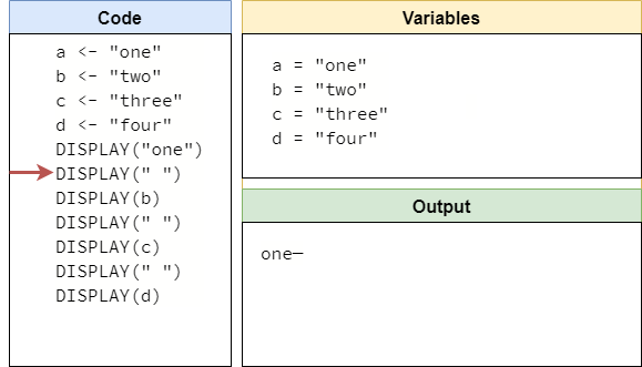
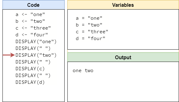
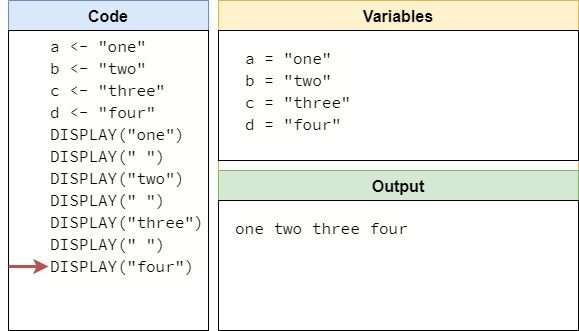
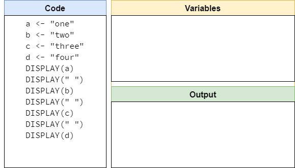
Our programs can also have multiple variables. In fact, there is no limit to the number of variables we can use - it just requires us to come up with a unique name for each one. For example, we could make a program that includes and displays multiple variables like this:
a <- "one"
b <- "two"
c <- "three"
d <- "four"
DISPLAY(a)
DISPLAY(" ")
DISPLAY(b)
DISPLAY(" ")
DISPLAY(c)
DISPLAY(" ")
DISPLAY(d)
This is a pretty complex program - one of the most difficult we’ve seen so far! To work out what it does, we can use a technique called code tracing. Let’s see how it works!
Code tracing involves mentally walking through the code line by line and recording what each line does. So, we’ll need to keep track of the current values of each variable, as well as the current output that is displayed to the user. We can easily do this by making a couple of boxes on a sheet of paper or in a couple of tabs of a text editor. For this example, we’ll use a simple graphic like this one:
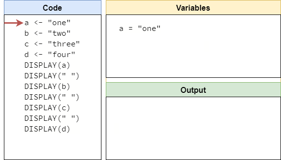
As we run the program, we’ll keep track of which line of code we are on, and update the trace as we go. So, let’s start by running the first line of code, a <- "one". When we run this line, we’ll need to create a new variable named a and store the value "one" in it. In our code trace, we can simply add an entry to the variables section as shown below:
There is no right or wrong way to record variables in our code trace. We can use boxes for each value and update it as we go, or just write a short text entry as shown in our example. Any method is valid. In the meantime, we’re using an arrow to keep track of which line we are running in our program, but we can just as easily do so with a finger or other tool in the real world!
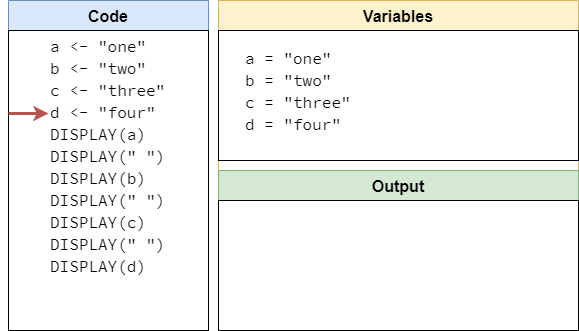
Looking at the next three lines of code, we see that they are all similar. So, we can quickly run them and populate the next four entries in our variables box:
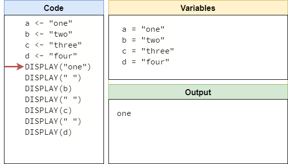
Now we’ve reached the first DISPLAY(expression) statement in our program. If we recall the way those statements work, we should first evaluate the expression into a value. In our code, our expression is the variable a, which isn’t a value. So, we need to evaluate it by looking up the current value of a and placing it in the current line of code. Then, we can display that value in the output. So, once we’ve run that line of code, our code trace will look something like this:
The next line of code is just DISPLAY(" "), which is simple since the expression " " is just a string value that doesn’t need to be evaluated. So, we’ll need to add a space to the end of our output. This can be tricky, since we really can’t “see” spaces. For now, we’ll just place a dash - in that space until we get the next piece of output.
Now we are back to a line that contains a variable. So, once again we look at the current value of the variable, place it in the expression, and then update our output. Since we’ve now received more output, we can remove that dash to make it a bit clearer.
From here on out, it should be pretty simple to figure out how the rest of this trace goes. When we are finished, we should have a code trace that looks like this:
The whole process is shown below in animated form:
Code tracing is a great way to train our “mental model” to work just like a real computer. While this may seem like a slow and tedious process right now, remember all of the other things we’ve learned how to do. Reading is initially very difficult, but with time and practice we can go from recognizing individual letters, to sounding out words, and finally reading with ease! The same happens as we learn to program and read code - with practice we’ll be able to do this in our head quickly and easily!
Let’s look at one more difficult concept in programming - using variables in the expressions for other variables. Right now we haven’t learned any operators (don’t worry - we’ll cover those in great detail in a future lab), but it is still important for us to understand what happens when we use the value in one variable to create or update the value in another variable.
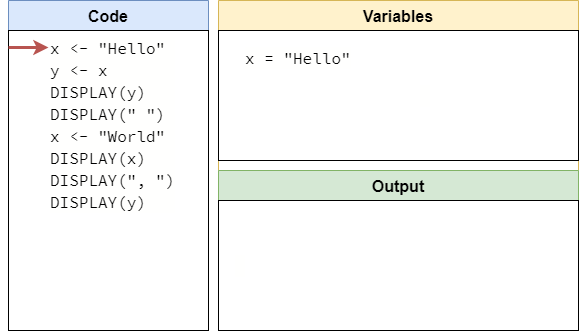
Let’s consider this program:
x <- "Hello"
y <- x
DISPLAY(y)
DISPLAY(" ")
x <- "World"
DISPLAY(x)
DISPLAY(", ")
DISPLAY(y)
To work out what this program displays, we can once again use code tracing to work through it line by line. The first line is pretty easy - we see that we are simply storing the string value "Hello" in a new variable named x, so we can easily update that on our code trace as shown below:
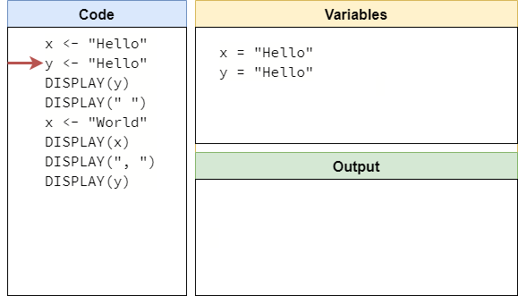
The next line is tricky - here we are storing the expression x into the variable named y. As before, we first have to evaluate the expression x to a value, which is simply the value stored in that variable. So, in actuality, we are storing the string value "Hello" in the variable y as well.
This is important to understand! In the code, and indeed in our “mental model” of a computer, we might start to think that the values stored in variable x and y are connected somehow. However, this is not the case. What the line y <- x says is simply that y now stores a copy of the value that was stored in x when this line is run. Going forward, these two values are not connected in any way, as we’ll soon see.
So, after running the second line of code, our code trace should now look like this:
The next two lines are pretty simple, since they only display the value stored in y followed by a space. So, after running those two lines, we should see the following on our code trace:
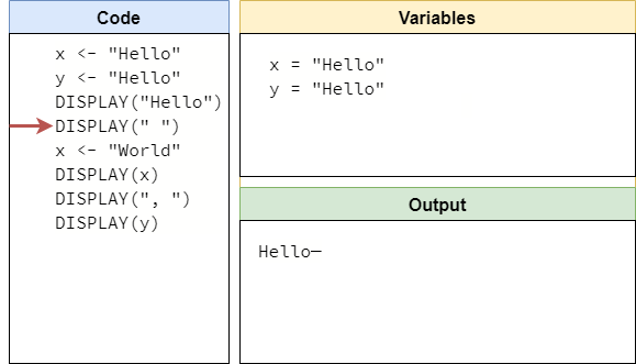
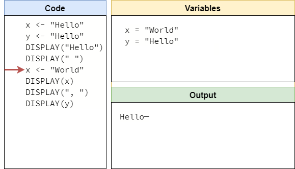
Now we reach the most important line, x <- "World". When we run this line, we’ll update the value stored in x to be the string value "World". However, this will not change the value stored in y. This is because y stores a copy of the value that was previously stored in x, and any changes to the value stored in x will not impact the value stored in y at all. So, after running that line, our code trace should show the following:
Once we’ve done that, running the next three lines of code is pretty straightforward. We’ll just display the current value stored in in x and y, with a comma and space between them. So, at the end, our code trace should look like this:
The entire trace can be seen in the animation below:
As we have learned, code tracing is a very important skill, and it helped us discover one of the most important rules about working with variables: when we assign the value of one variable into another, we copy the existing value, but those two variables are not related to each other after the fact.
In this lab, we’re going to take what we’ve learned in pseudocode and see how it transfers to a real programming language, Python. We’ve chosen Python because it is very easy to learn, easy to use, and it is used in many different places, from scientific computing and data analysis to web servers and even artificial intelligence. It is a very useful language to learn, and it makes a great first programming language.
We’ve already built a pretty effective “mental model” of a computer by working in pseudocode. So, as we work through this lab, we’ll need to constantly pay attention to how a real computer works, and make sure that our “mental model” is accurate. If not, we’ll have to adapt our understanding of a computer to match the real world. This process of adaptation and accommodation is an important part of learning to program - we have to have a good understanding of what a computer actually does when it runs our code, or else we won’t be able to write code that will do what we want it to do.
As we learn to write code in a real programming language, it helps to refer to the actual documentation from time to time. So, we recommend bookmarking the official Python Documentation as a great place to start. Throughout this course, we may also include links to additional resources, and those are also worth bookmarking. One of the best parts about programming is that nearly all of the documentation is online and easily accessible, and learning how to quickly search for a particular solution or reference is just as useful as knowing how to do it from memory. In fact, most programmers really only know the basics of the language and a few handy tricks, and the rest of it is just reading documentation and learning when to use it. So, don’t worry about remembering it all right from the start - instead, learn to read the documentation and use the tools that are available, and focus on understanding the basics of the language’s syntax and rules.
First, let’s start with the basics of writing Python code in a file and running those files. This is the first major step toward actually writing a real program, but it can definitely be difficult the first time without prior experience to rely on. So, let’s go through it step by step and make sure we know how to run our programs in Python.
At this point, we should already have Python installed on our system. For students using Codio, this is taken care of already. For students using their own computers, refer to an earlier lab to find instructions for installing Python on your system, or contact the instructors for assistance.
To make sure that Python is installed and working, we’ll need to open a terminal in our operating system. In Codio, this can be found by clicking the Tools menu at the top, and then choosing Terminal. More information can be found in the Codio Documentation . There may also already be one open for you if you are reading this content from within Codio.
If you are working on your own computer, you’ll need to open a terminal on your operating system. This should have been covered in the previous lab when you installed Python. On Windows, look for Windows Terminal or Windows PowerShell (not the old Command Prompt, which requires different commands). On Mac or Linux, look for an application called Terminal. Throughout this course, we’ll call these windows the terminal, even though they may have slightly different names in each operating system.
Once we have the terminal open, we should see something like one of these examples:


At this point, we should see a place with a blinking cursor, where we can type our commands. This is called the command prompt in the terminal. The first thing we can do is check to make sure Python is properly installed, and we can also confirm that it is the correct version. To do this, we’ll enter the following command and press enter to execute it:
python3 --versionHopefully, that command should produce some output that looks like this:
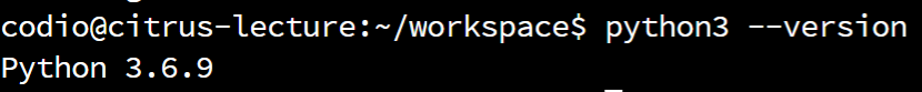
Here, we see that the currently installed Python version is 3.6.9. As long as your Python version number begins with a 3, you have correctly installed Python and are able to run it from the terminal. So, we can continue to the next part of this lab.
If you aren’t able to run Python or aren’t sure that you have the correct version, contact the instructor for assistance!
Notice that we have to use the command python3, including the version number, instead of the simpler python command here. This is because some systems may also have Python version 2, an outdated version of Python, installed alongside version 3. In that case, the simple python command will be Python version 2, while python3 will be Python version 3. Unfortunately, most programs written in Python 3 will not run properly in Python 2, so it is important for us to make sure we are using the correct Python version when running our programs.
Thankfully, the command python3 should always be Python version 3, and using that command is a good habit to learn. However, depending on how Python is installed on Windows, it might only work via the python command, which can make it confusing. So, throughout this course, we will use the command python3 to run Python programs, but you may have to adapt to your particular situation.
When we open a terminal, it will usually start in our user’s home folder. This may mean different locations for different operating systems. For example, if our current user’s name is <username>, the terminal will usually start in this location for each operating system:
C:\Users\<username>/home/<username>/Users/<username>/home/codio/workspaceThe directory that is open in the terminal is known as the working directory. We can use the pwd command to determine what our current directory is:
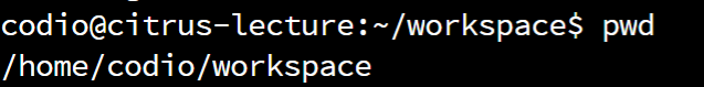
In this example, we are looking at the Codio terminal, so our working directory is /home/codio/workspace.
Next, we can see the files and directories contained in that directory using the ls command. Here’s the output of running this command in Codio:
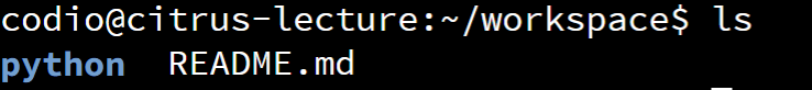
In the output, we can see that there is a file named README.txt and a directory named python. In Codio, we’ll place all of our files in the python directory, so we can open that using the cd python command:
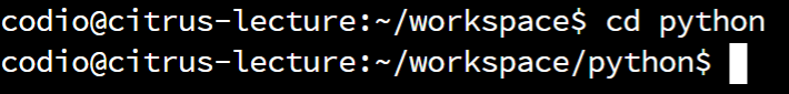
Notice how the python directory is now included in the command prompt in the terminal. Most terminals will show the working directory in the command prompt in some way.
That’s the basics of navigating in the terminal, but there is much more to learn. If you’d like to know more, consider checking out some of the resources linked below!
Most of the content in this course will focus on using the commands that are present in the Linux terminal, since they are the most widely-used commands across all platforms. In general, these commands should work well on both Windows and Mac, with a few caveats:
Fully learning how to use these tools is outside of the scope of this class, but we need to know enough to navigate the filesystem and execute the python3 command. If you need assistance getting started with this step, your best bet is to contact the instructors. Each student’s computer is a bit different, so it is difficult to cover all possible cases here.
The first statement that we’ll cover in the Python programming language is the print(expression) statement. This statement is used to display output to the user via the terminal. So, when Python runs this statement, it will evaluate the expression to a single value, and then print that value to the terminal.
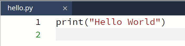
For example, the simplest Python code would be a simple Hello World program, where we use the print(expression) statement to display the text "Hello World" to the user:
print("Hello World")When we run that program in Python, we’ll see the following output:
Hello WorldJust like in pseudocode, strings in Python are surrounded by double-quotes ". For now, we’re just going to work with string values, but in a later lab we’ll introduce numerical values and discuss how to use them as well.
Let’s go through the full process of writing and running that program in Python!
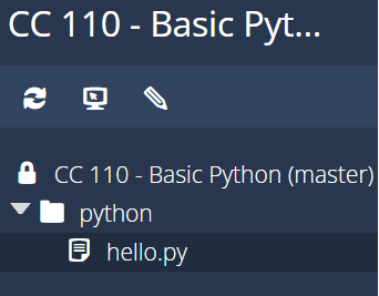
The first step to create a program in Python is to create a text file to store the code. This file should have the file extension .py to indicate that it is a Python program. So, we’ll need to create that file either on our computers or in Codio or another tool if we are using one. For example, in Codio we can create the file in the python folder by right-clicking on it and selecting the New File option. We’ll name the file hello.py:
Once we’ve created that file, we can then open it by clicking on it. In Codio and in other online tools, it will open in the built-in editor. On a computer, we’ll need to open it in a text editor specifically designed for programming. We recommend either Atom or Visual Studio Code , which are available on all platforms. Tools like the built-in Notepad tool on Windows, or a word processor like Word or Pages do not work for this task.
In that file, we’ll simply place the code shown above, like this:
That’s all there is to it!
Once we’ve written the code, we can open the Terminal and navigate to where the code is stored in order to run the program. On Codio, we’ll just use the cd python command to enter the python directory. On a computer, we’ll need to navigate the file system to find the location where we placed our code. We highly recommend creating a folder directly within the home directory and placing all of our code there - that will make it easy to find!
Once we are in the correct directory, we can use the ls command to see the contents of that directory. If we see our hello.py file, we are in the correct location:
If we don’t see our file, we should make sure we’ve saved it and that our current working directory is the same location as where the file is stored.
Finally, we can execute the file in Python using the python3 command, followed by the name of the file:
python3 hello.pyIf everything works correctly, we should see output similar to this:
There we go! We’ve just run our first program in Python! That’s a great first step to take.
Of course, there are lots of ways that this could go wrong. So, if you run into any issues getting this to work, please take the time to contact an instructor and ask for assistance. This process can be daunting the first time, since there are so many things to learn and so many intricacies we simply don’t have time to cover up front. Don’t be afraid to ask for help!
The print(expression) statement in Python works in much the same way as the DISPLAY(expression) statement in pseudocode, but with one major difference. In pseudocode, the DISPLAY(expression) statement will print the value from the expression to the user, but it won’t add anything like a space or newline to the end. In Python, however, the print(expression) statement will add a newline to the end of the output by default. This means that multiple print(expression) statements will print on multiple lines. Let’s look at some examples!
Throughout this course, we’ll show many different code examples and their output here in the lab. To test them out, feel free to copy the code examples to a Python file and run it yourself. You can even tweak them to do something new and see how Python interprets different pieces of code. In the end, the best way to learn programming is to explore, and running these examples on your own is a great way to get started!
In Python, we can print multiple lines of output simply by using multiple print(expression) statements:
print("a")
print("b")
print("c")
print("d")
will result in this output:
a
b
c
d
We can also include a newline symbol \n in a print(expression) statement in Python. This will add a newline to the output, and then the print(expression) statement will add an additional newline at the end of the value that is printed:
print("one\ntwo")
print("three\nfour")
will produce this output:
one
two
three
fourWhat if we want to display multiple print(expression) statements on the same line? To do that, we must add an additional option to the print(expression) statement - the end option.
For example, the following code will produce output all on the same line:
print("Hello ", end="")
print("World!")
In this example, we set end to be an empty string "". When we run this program, we’ll get the following output:
Hello World!In fact, in Python, the print(expression) statement is an example of a function in Python. Functions in Python are like procedures in pseudocode - when we call them, we write the name of the function, followed by a set of parentheses and then arguments separated by commas within the parentheses. So, in actuality, the expression in the print(expression) statement is just the first argument when we call the print function.
Therefore, the end option that we showed above is just a second argument that is optional - it simply let’s us choose what to put at the end of the output. By default, the end parameter is set to the newline symbol \n, so if we don’t provide an argument for end it will just add a newline at the end of the value.
We can set the value of end to be any string. If we want to include a space at the end of the output, we can add end=" " to the print function call.
In this course, we won’t spend much time talking about optional parameters and default values in Python functions, but it is important to understand that statements like print are actually just Python functions behind the scenes!
As we learn to write more complex programs in Python, it is important to make sure we can still mentally execute the code we are writing in our “mental model” of a computer before we actually run it on a computer. After all, if we don’t have at least an idea of what the code actually does before we write it, we really haven’t learned much about programming!
Thankfully, when working in a real programming language such as Python, there are many tools to help us visualize how the code works when we run it. This helps us continue to develop our “mental model” of a computer by looking behind the scenes a bit to see what is happening when we run our code.
One such tool is Python Tutor , a website that can quickly run short pieces of Python code to help us visualize what each line does and how it works. This tool is also integrated directly into Codio!
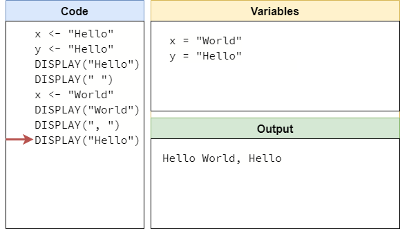
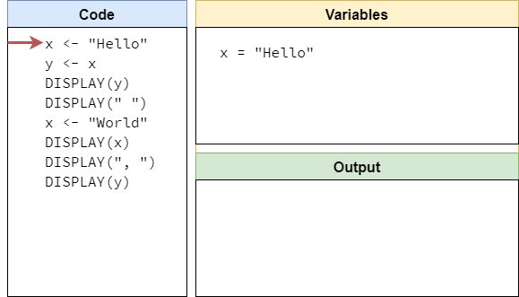
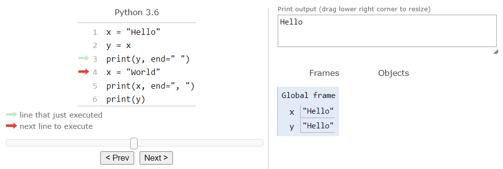
Let’s look at an example of how Python Tutor compares to the manual code traces we performed in a previous lab. For this example, we’re going to use the following code:
x = "Hello"
y = x
print(y, end=" ")
x = "World"
print(x, end=", ")
print(y)
In Codio, we can see the visualization in a tab to the left. It will visualize the content in the tutor.py file in the python directory, so make sure that the contents of the tutor.py file match the example above before continuing.
Outside of Codio, this visualization can be found by clicking this Python Tutor Link to open Python Tutor on the web.
The initial setup for Python Tutor is shown in the image below:

This looks similar to the setup we used when performing code tracing with pseudocode. We have an arrow next to our code that is keeping track of the next line to be executed, and we have areas to the side to record variables and outputs. In Python Tutor, the variables are stored in the Frames section. We’ll learn why that is important later in this lab when we start looking at Python functions.
So, let’s click the Next > button once to execute the first line of code. After we do that, we should see the following setup in Python Tutor:
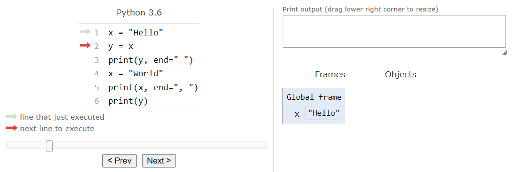
That line is an assignment statement, so Pyhton Tutor added an entry in the Frames section for the variable x, showing that it now contains the string value "Hello". It placed that variable in a frame it is calling the “Global frame,” which simply contains variables that are created outside of a function in Python.
When we click the Next > button again, we should see this:
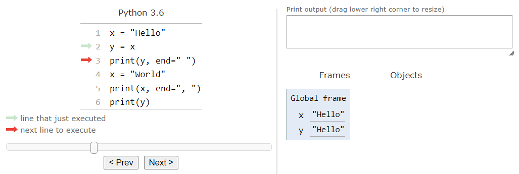
Once again, the line that was just executed is an assignment statement, so Python Tutor will add a new variable entry for y to the list of variables. It will also store the string value "Hello". Just like before, notice that the variable y is storing the same value as x, but it is a copy of that value. The variables are not connected in any other way.
We can click Next > again to execute the next line of code:
Once this line is executed, we’ll see that it prints the value of the variable y to the output. Python Tutor will look up the value of y in the Frames section and print it in the output, but it won’t evaluate the expression in the code like we did when we performed code tracing in pseudocode. It’s a subtle difference, but it is worth noting.
Once again, we can click Next > to execute the next assingment statement:
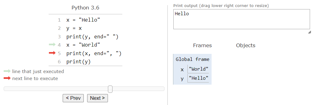
This statement will update the value stored in the variable x to be the string value "World". After that, we can run the next statement:
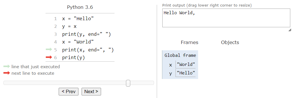
That statement prints the value of x to the output, followed by a comma , and a space as shown in the end argument provided to the print function. Finally, we can click Next > one more time to execute the last line of code:
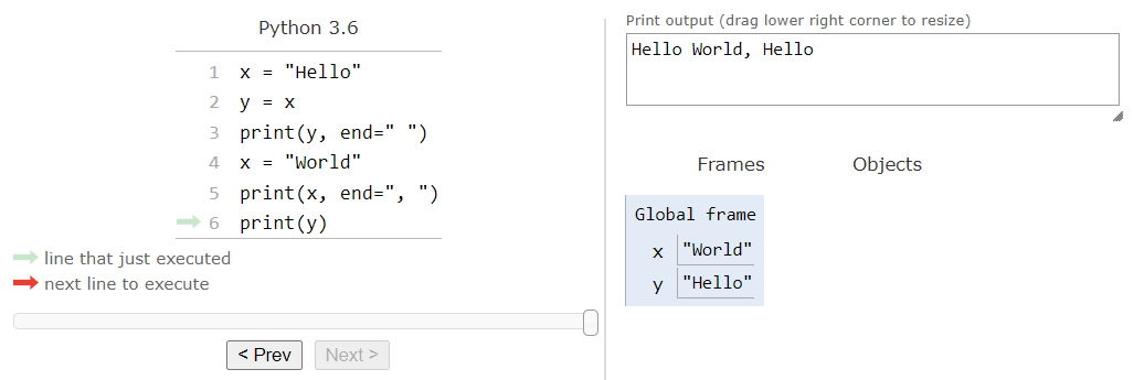
This will print the value of y to the output. Once the entire program has been executed, we should see the output Hello World, Hello printed to the screen.
The full process is shown in the animation below:
Using tools like Python Tutor to step through small pieces of code and understand how the computer interprets them is a very helpful way to make sure our “mental model” of a computer accurately reflects what is going on behind the scenes when we run a piece of Python code on a real computer. So, as we continue to show and discuss examples in this course, feel free to use tools such as Python Tutor, as well as just running the code yourself, as a great way to make sure you understand what the code is actually doing.
In this lab, we introduced a simple pseudocode programming language, based on the one used by the AP Computer Science Principles exam. This pseudocode language includes several statements and rules we’ve learned to use in this lab. Let’s quickly review them!
The DISPLAY(expression) statement is used to display output to the user.
expression to a value, then display it to the screen.DISPLAY(" "), and we can use the newline symbol to go to the next line DISPLAY("\n")The assignment statement, like a <- expression is used to create variables and store values in the variables.
This pseudocode language may seem very simple, but we’ve already learned a great deal about how programming works and how a computer interprets a program’s code, just by practicing with this very simple language. In the next lab, we’ll see how these concepts directly relate to a real programming language, Python. For now, feel free to keep practicing by writing programs and pseudocode and running them on your “mental model” of a computer. It is a very important skill to develop!
We also introduced some basic statements and structures in the Python programming language. Let’s quickly review them!
The print(expression) statement is used to print output on the terminal.
expression to a value, then display it to the screen.end parameter, such as print(expression, end="") to remove the newline.The assignment statement, like a = expression is used to create variables and store values in the variables.
As we’ve seen, the Python language is very similar to the pseudocode language we’ve already learned about. Hopefully the practice we have in reading and writing pseudocode using our “mental model” of a computer will help make it even easier to read and write Python code that is meant to be run on an actual computer.
As our programs get larger and larger, we’ll probably find that we keep repeating pieces of code over and over again in our programs. In fact, we’ve probably already done that a few times just working through this lab. What if we had some way to build a small block of code once, and then reuse it over and over again in our programs?
Thankfully, this is a core feature of most programming languages! In our pseudocode, we call these procedures, though many other programming languages refer to them as functions, methods, or subroutines. For now, we’ll use procedure in pseudocode, and later on we’ll introduce the same concept in Python using a different term.
Creating a procedure requires a more complex structure in our code than we’ve seen previously. The best way to learn it is to just see it in action, so here is the basic structure of a procedure in pseudocode:
PROCEDURE procedure_name()
{
    <block of statements>
}
Let’s look at each part of this structure in detail to see how it works:
PROCEDURE. Just like DISPLAY, the PROCEDURE keyword is a built-in part of our language that we use to create a new procedure.PROCEDURE we see the name of the procedure. In this case, we are using procedure_name as the name of the procedure. Procedure names follow the same rules and conventions as variable names that we discussed earlier. The two most important rules are:
(). These are used for the parameters of a procedure, which we’ll learn about on the next page.{ on the next line, and a closing curly brace } a few lines later. The curly braces are used to define the block of statements that make up the procedure.<block of statements> section. This is where we can place the code that will be run each time we run this procedure. Each procedure will include at least one statement here, but many times there are several.It may seem a bit complex at first, but creating a procedure is really simple. For example, let’s see if we can create a procedure that performs the “Hello World” action we learned about earlier. We’ll start by writing the keyword PROCEDURE followed by the name hello_world, some parentheses, and a set of curly braces:
PROCEDURE hello_world()
{

}
That’s the basic structure for our procedure! Now, inside of the curly braces, we can place any code that we want to run when we use this procedure. To make it easier to read, we will indent the code inside of the curly braces. That makes it clear that these statements are part of the procedure, and not something else. So, let’s just have this procedure display "Hello World" to the user:
PROCEDURE hello_world()
{
    DISPLAY("Hello World")
}
There we go! That’s what a basic procedure looks like.
Of course, learning how to write a procedure is only part of the process. Simply creating a procedure doesn’t actually cause it to run. So, once we have a procedure created, we have to learn how to use it in our code as well.
When we want to run a procedure, we call it from our code using its name. It may seem strange at first, but the term call is what we use to describe the process of running a procedure in our code.
Thankfully, a procedure call is very simple - all we have to do is state the name of the procedure, followed by a set of parentheses:
hello_world()So, our complete program would include both the definition of our procedure, and then a procedure call that executes it. Typically, we include the procedure calls at the bottom of the program, so it would look like this:
PROCEDURE hello_world()
{
    DISPLAY("Hello World")
}

hello_world()
Pretty simple, right? To make our code easy to read, we usually leave a blank line after the creation of a procedure, as shown in this example.
When our “mental model” of a computer runs this code, it will start at the top. Here, it sees that we are creating a procedure called hello_world, so it will make a note of that. It won’t run the code inside the procedure just yet, but it will remember where that procedure is in our code so it can find it later. It will then jump ahead to the end of the procedure, marked by the closing curly brace }. As it moves on from there, it will see the line that is a procedure call. Since it knows about the hello_world procedure, it can then jump to that place in the code and run that procedure before jumping back down here to run the next line of code. However, it can be a bit tricky to follow exactly what is going on, so let’s go through a code tracing exercise to make sure our “mental model” of a computer can properly follow procedure calls in our programs.
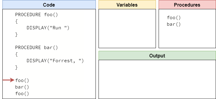
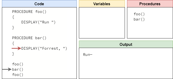
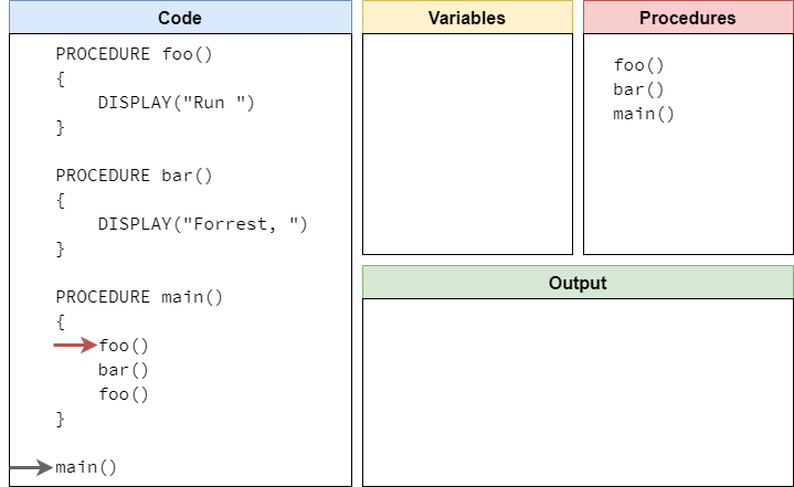
Let’s consider the following program, which contains two procedures, and a bit of code to call those procedures:
PROCEDURE foo()
{
    DISPLAY("Run ")
}

PROCEDURE bar()
{
    DISPLAY("Forrest, ")
}

foo()
bar()
foo()
As before, we can set up our code tracing structure that includes our code, variables, and output. However, this time we’re also going to add a new box to keep track of the procedures in our program. So, our code tracing structure might look something like this:
Once again, we can work through this program line by line, starting at the top. In this program, the very first thing we find is the creation of a new procedure. At this point, we aren’t running the code inside the procedure, we are simply creating it. So, our program will record that it now knows about the procedure named foo in its list of procedures, and it will skip down to the next line of code after the procedure is created.
This line is just a blank line, so our “mental model” of a computer will just skip it and move to the next line. Blank lines are simply ignored by the computer, but it makes it easier for us to write code that is readable. So, on the next line, we see the creation of another procedure:
Once again, we see that a new procedure is being created, so our computer will simply make a note of it and move on. It will skip the blank line below the procedure, and eventually it will reach the first procedure call, as shown below:
Ok, here’s where things get a bit tricky! At this point, we are calling the procedure named foo. So, our computer will check the list of procedures it knows about, and it will see that it knows where foo() is located. So, our “mental model” of a computer knows that it can execute that procedure. To do that, it will jump up to the first statement inside of the procedure and start there. At the same time, it will also keep track of where it was in the program, so it can jump back there once the procedure is done. We’ll represent that with a shaded arrow for now:
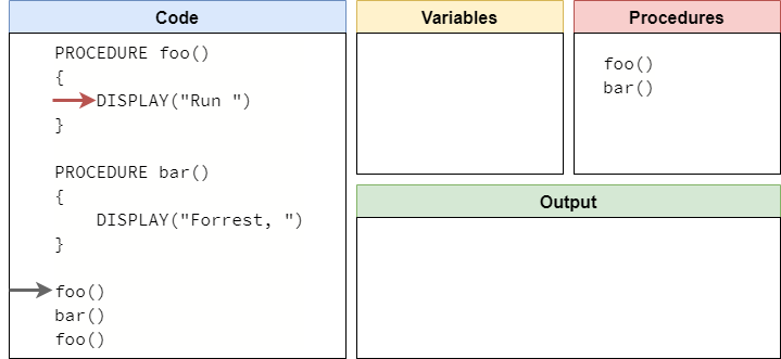
Now we are looking at the first line of the foo procedure, which simply displays the text "Run " on the output. So, we’ll update our output, and move to the next line of the procedure.
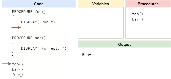
At this point, we’ve reached the end of our procedure. So, our computer will then jump back to the previous location, indicated by the shaded arrow.

Since there is nothing else to execute on this line, it will simply move to the next line.
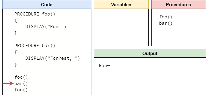
Once again, we see that this is another procedure call. So, the computer will make sure it knows where the bar() procedure is, and then it will jump to the first line of that procedure. When it does, it will remember what line of code it was currently running, so it can jump back at the end of the procedure.
Like before, it will then run the first line of the bar() procedure, which will display "Forrest, " to the user. So, we’ll update our output section, and move the arrow to the next line.
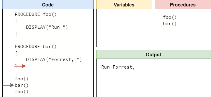
We’re back at the end of a procedure, so we will jump back to the previous location and see if there is anything else to do on that line:

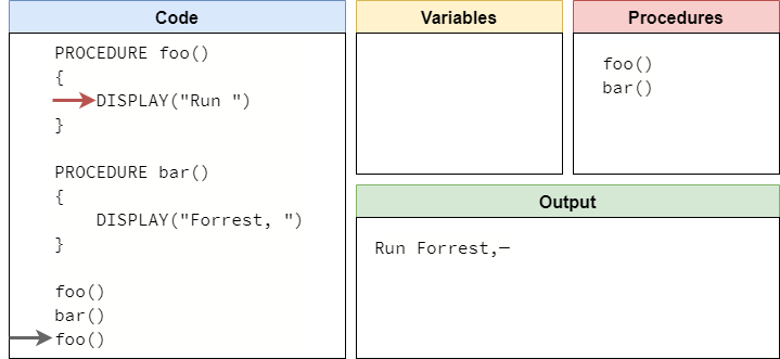
Since there’s nothing else there, our “mental model” will just move to the next line of code:

By now, we should have a good idea of what is happening when we call a procedure. We simply jump to where it starts, making sure we remember where we came from:
Then, we execute the lines of code in the procedure:
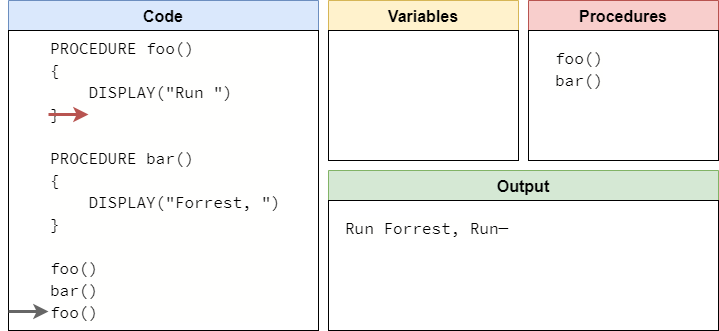
Finally, when we reach the end of the procedure, we go back to where we came from and see if there is anything else to do on that line:
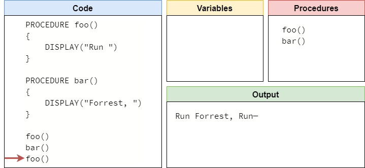
There’s nothing left to do, so we’ve reached the end of our program! The full process is shown in the animation below:
It is very important for us to make sure our “mental model” of a computer knows how to properly call and execute procedures, since that is a core part of developing larger and more complex programs. Thankfully, we’ll get lots of practice at this as we learn to program!
One of the tricky parts of learning how to program is knowing when to take a piece of code and make it into a procedure. A great principle to keep in mind is the Don’t Repeat Yourself or “DRY” principle of software development. In this principle, if we find that our program contains the same lines of code in multiple places, we should make a procedure containing those lines of code and call that procedure each time we use those lines in our program. In that way, we are only writing that block of code once, and we can use it anywhere.
Another principle is that programs should only consist of procedures, and each procedure should only be a few lines of code. By following this method of development, each procedure only performs one or two actions, making it much easier to test and debug those procedures independently and make sure they are working properly before testing the entire program as a whole.
As we continue to learn more about programming, we’ll see both of these principles in action.
Up to this point, we’ve simply written code and expected it to run easily in our “mental model” of a computer. However, many programming languages place one additional requirement on code that we should also follow: all code must be part of a procedure.
What does this mean? Put simply, we shouldn’t place any code in our programs that isn’t part of a procedure. Or, put another way, our programs should only consist of procedures and nothing else.
But wait! Didn’t we just learn that our “mental model” of a computer will just skip past procedures when it runs our programs, and it will only execute the code inside of a procedure when it is called? How can we call a procedure if all of our code must be within a procedure? It sounds a bit like a “chicken and egg” problem, doesn’t it?
Thankfully, there is a quick and easy way to solve this. Many programming languages define one specific procedure name, usually main, as the defined starting point of a program. In those languages, the computer often handles calling the main procedure directly when a program starts. Other languages don’t define this as a rule, but many developers choose to follow it as a convention. In our pseudocode, we will follow this convention, since this closely aligns with the Python language we’ll learn later in the course.
Let’s see an example. We can update the example on the previous page to include a main procedure by simply placing all of the code at the bottom of the program into a procedure. We’ll also include a call to the main procedure at the bottom of the code, as shown below:
PROCEDURE foo()
{
    DISPLAY("Run ")
}

PROCEDURE bar()
{
    DISPLAY("Forrest, ")
}

PROCEDURE main()
{
    foo()
    bar()
    foo()
}

main()
That’s really all there is to it! From there, our “mental model” of a computer will know that it should start executing the program in the main procedure. Let’s quickly code trace the first part of that process, just to see how it works. As before, we’ll start running our program at the top of the code:

Just like we saw previously, this line is creating a new procedure named foo. So, we’ll make a note of that procedure, and move on to the next part of the code:
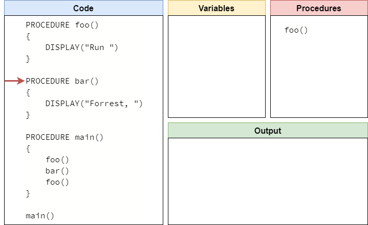
Here, we are creating the bar procedure, so we’ll record it and move on:

Likewise, we see the creation of the main procedure, so we’ll record it and continue working through the program:
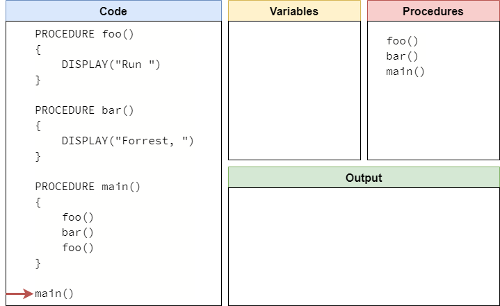
Finally, we’ve reached the end of the code, and here we see the call for the main procedure. So, just like we saw before, our “mental model” of a computer will determine that it has indeed seen the main procedure, and it will jump to the start of that procedure:
From here, the rest of the program trace is pretty much the same as what we saw before. It will work through the code in the main procedure one line at a time, jumping to each of the other procedures in turn. Once it reaches the end of the main procedure, it will jump back to the bottom of the program where main is called, and make sure that there is nothing else to execute before reaching the end of the program. The full process is shown in the animation below:
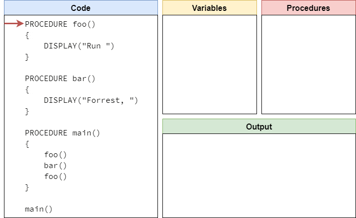
From here on out, we’ll follow this convention in our programs. Specifically:
main as the starting point of the program.main procedure at the bottom of the program.These conventions will help us write code that is easy to follow and understand. We’ll also be learning good habits now that help us write code in a real programming language, such as Python, in a later lab.
The last new concept we’re going to introduce in this lab is the concept of parameters. We just learned how to create procedures in our code, but our current understanding of procedures has one very important flaw in it: a procedure will always do the same thing each time we call it! What if we want to write a procedure that performs the same operation, but uses different data each time? Wouldn’t that be useful?
Thankfully, we can do just that by introducing parameters into our procedures. A parameter is a special type of variable used in a procedure’s code. The value of the parameter is not given in the procedure itself - instead, it is provided when the procedure is called. When a value is given as part of a procedure call, we call it an argument. So, a procedure has parameters, and the value of those parameters is given by arguments that are part of the procedure call.
To include parameters as part of a procedure, we simply list the names of the parameters in the parentheses after the procedure name. If we want to use more than one parameter, we can separate them using a comma ,. Here’s an example of a "Hello World" procedure that uses two parameters:
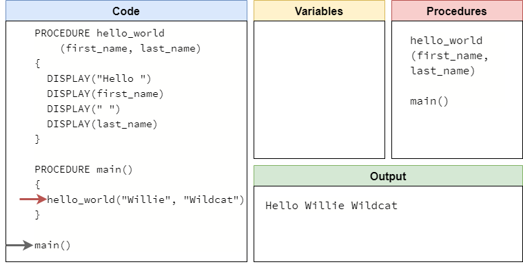
PROCEDURE hello_world(first_name, last_name)
{
    DISPLAY("Hello ")
    DISPLAY(first_name)
    DISPLAY(" ")
    DISPLAY(last_name)
}
Inside of the procedure, we can use first_name and last_name just like any other variable. We can read the value stored in the variable by using it in an expression, and we can even change the value stored in the variable within the procedure itself using an assignment statement.
Now that we have a procedure that requires parameters, we need to call that procedure by providing arguments as part of the procedure call. To do that, we provide expressions that result in a value inside of the parentheses of a procedure call. Once again, multiple arguments are separated by commas.
For example, we can call the hello_world procedure by providing two arguments like this:
hello_world("Willie", "Wildcat")So, when this code is run on our “mental model” of a computer, we should receive the following output on the user interface:
Hello Willie WildcatLet’s walk through a quick code trace to see exactly what happens when we call a procedure with arguments.
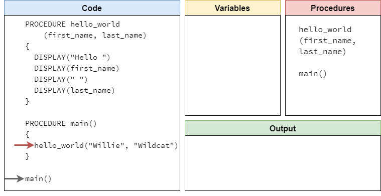
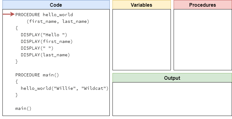
First, let’s formalize the example above into a complete program:
PROCEDURE hello_world(first_name, last_name)
{
    DISPLAY("Hello ")
    DISPLAY(first_name)
    DISPLAY(" ")
    DISPLAY(last_name)
}

PROCEDURE main()
{
    hello_world("Willie", "Wildcat")
}

main()
To do that, we’ve placed our procedure call in a main procedure, and we’ve added a call to the main procedure at the end of our program. So, once again, we can set up our code trace structure to include our code and the various boxes we’ll use to keep track of everything:
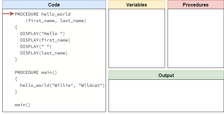
We are already pretty familiar with how our “mental model” of a computer will scan through the whole program to find the procedures, so let’s skip ahead to the last line with the procedure call to main:
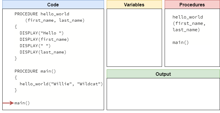
Once again, our computer will see that it is calling the main procedure, which it knows about. So, it will jump to the beginning of the main procedure and start from there:
This line contains another procedure call, this time to the hello_world procedure. However, when our “mental” computer looks up that procedure in its list of procedures, it notices that it requires a couple of parameters. So, our computer will also need to check that the procedure call includes a matching argument for each parameter. In our pseudocode language, each parameter must have a matching argument provided in the procedure call, or else the computer will not be able to run the program.
Thankfully, we see that there are two arguments provided, the values "Willie" and "Wildcat", which match the two parameters first_name and last_name. So, the procedure call is valid and we can jump to the beginning of the procedure.
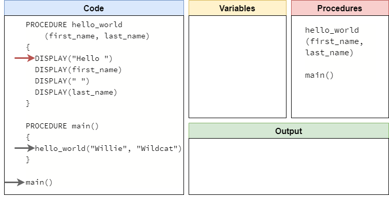
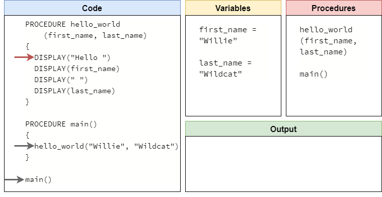
This time, however, we’ll need to perform one extra step. When we call a procedure that includes parameters, we must also list the parameters as variables when we start the procedure. The value of those variables will be the matching argument that was provided as part of the procedure call. So, the parameter variable first_name will store the value "Willie", and the parameter variable last_name will store the value "Wildcat". Therefore, our code trace should really look like this when we start running the hello_world procedure:
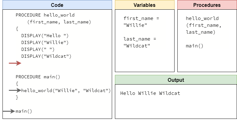
In the future, we’ll show that as just one step in our code trace. Once we are in the hello_world procedure, we can simply walk through the code line by line and see what it does. At the end of the procedure, we’ll see that it has produced the expected output:
At this point, we will jump back to the main procedure. When we do this, there are a couple of other things that happen in our “mental model” of a computer:
hello_world procedure are removed. This includes any parameter variables.So, after that step, our code trace should look like this:
Now we are back in the main procedure, and the program will simply reach the end of that procedure, then jump back to the main procedure call and reach the end of the program. The full code trace is shown in the animation below:
That’s all there is to calling a procedure that uses parameters! We can easily work through it using the code tracing technique we learned earlier in this lab.
The definitions for parameter and argument given above are the correct ones. However, many programmers are not very precise about how they use these terms, so in practice you may see the terms parameter and argument used somewhat interchangeably.
We’ll do our best to use them correctly throughout this course, and we encourage you to be careful about how you use the terms and make sure you understand the difference.
Let’s briefly consider one more important situation that may arise when calling procedures. What if the arguments provided in a procedure call are variables themselves? What does that look like?
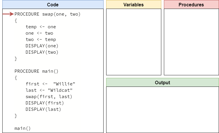
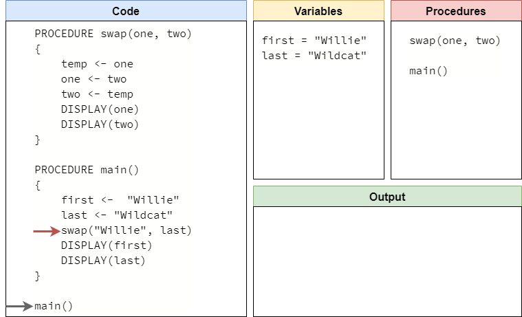
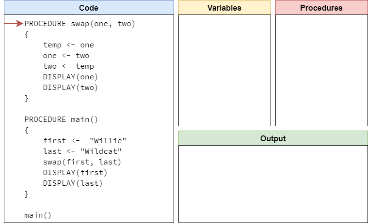
Let’s work through an example:
PROCEDURE swap(one, two)
{
    temp <- one
    one <- two
    two <- temp
    DISPLAY(one)
    DISPLAY(two)
}

PROCEDURE main()
{
    first <-  "Willie"
    last <- "Wildcat"
    swap(first, last)
    DISPLAY(first)
    DISPLAY(last)
}

main()
Before reading the code trace below, take a moment to read this code and see if you can predict what the output will be.
Like before, let’s set up our code trace to include our code and the various boxes we need to keep track of everything:
Let’s go ahead and skip to the bottom where the main procedure call is. When we reach that line, we’ll start at the top of the main procedure, like this:
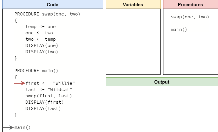
Next, we can move through the following two lines of code, which create the variables first and last, storing the values "Willie" and "Wildcat", respectively. At this point, we’re ready to call the swap procedure:

To make a procedure call, we must first make sure the computer knows about the procedure. Since it is in our procedures box, we know we’ve seen it. The next step is to check and make sure that there is a matching argument for each parameter. The swap procedure requires two parameters, and we’ve provided two arguments, so that checks out. The next step is to actually evaluate each of the expressions used as arguments to a single value. If we look at our code, we see that the first argument expression is the variable first, which stores the value "Willie". So, we can place that value where the variable goes in our procedure call:
Then, we can do the same for the last variable, which stores the value "Wildcat":

Now that we’ve evaluated all of our argument expressions, we can finally perform the procedure call and enter the swap procedure. When we do this, we’ll create two new variables, one and two, and populate them with the values that we evaluated for each expression. Just like when we store the value of one variable into another, these are copies of the values that were stored in the original variables. So, just because they have the same value, they otherwise aren’t connected, as we’ll see later. So, our current code trace should look like this:
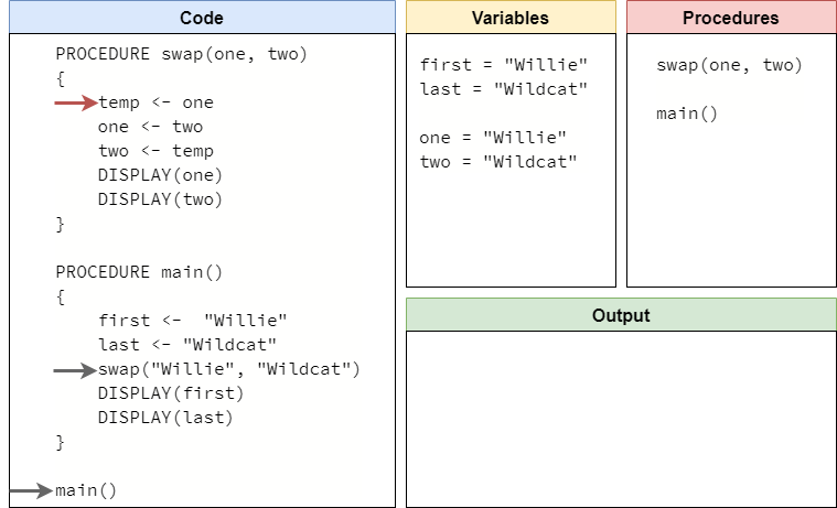
Inside of the swap procedure, we actually perform a three step “swap” process, which will swap the contents of the parameter variables one and two. First, we place the value of one in a new variable we call temp:

Next, we place the original value in two into one. At this point, they both have the same value, but we’ve stored the original value from one into temp, so it hasn’t been lost:
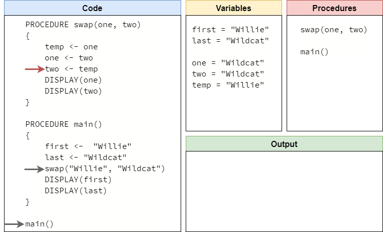
Finally, we can place the value from temp into two, completing the swap:
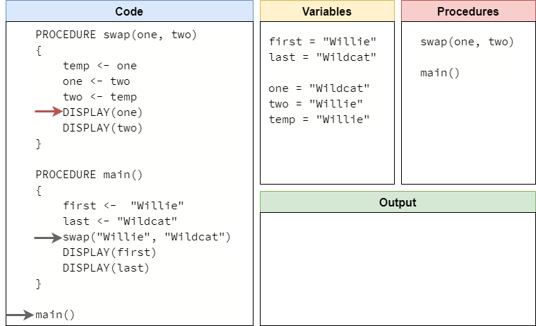
The next two lines will simply display the current values in one and two to the user:
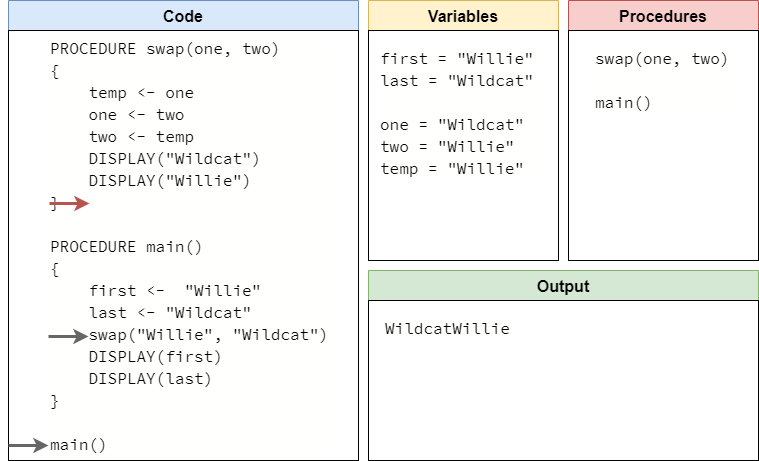
Notice that the values of first and last have not changed throughout this entire process. They are still the same values that were originally set in the main procedure. At this point, we’ve reached the end of the swap procedure. So, we can jump back to the location we left off in the main procedure. When we do so, we’ll remove all of the variables we created in the swap procedure. We’ll also reset all of the evaluated expressions in the swap procedure back to the original code. So, our code trace should now look like this:

Since there’s nothing else to evaluate on this line, we can move to the next line in the program:
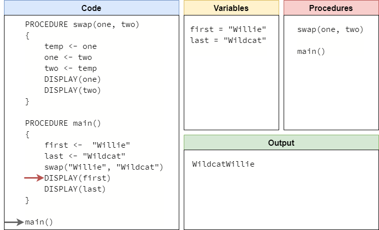
The next two lines are going to print the values of the first and last variables in the interface. Notice that, even though we swapped the values of one and two in the swap procedure, the values of first and last are unchanged here. This is an important concept to remember - when we use a variable as an argument in a procedure call, the procedure receives a copy of the value stored in that variable. So, any chagnes to the parameter variable in the procedure will not affect the variable that was used as an argument in the procedure call. In technical terms, we say this is a call by value procedure, since it uses the values in the arguments.
So, after running those two lines of code, we should reach the end of the main procedure, and our code trace should look like this:

At this point, we’re at the end of the main procedure, so the computer will just jump back to the main procedure call, and reach the end of the program! The whole process is shown in the animation below:
As we can see, calling procedures is a pretty easy process. By using parameters, we can build procedures that repeat the same steps in our program, just with different data each time.
Python also supports the use of procedures, which allows us to write small pieces of code that can be repeatedly used throughout our programs. In Python, we call these procedures functions. We’ve already seen one example of a function in Python - the print statement is actually a function! Let’s look at how we can create and use functions in Python.
The process of creating a function in Python is very similar to the way we created a procedure in pseudocode. A simple function in Python uses the following structure:
def function_name():
    <block of statements>
Let’s break this structure down to see how it works:
def, which is short for define. In effect, we are stating that we are defining a new function using the special def keyword._. Function names beginning with an underscore _ have special meaning, so we won’t use those right now._.(). This is where we can add the parameters for the function, just like we did with procedures in pseudocode. We’ll see how to add function parameters later in this lab.:. This tells us that the block of statements below the function definition is what should be executed when we run the function. In pseudocode, we used curly braces {} here.} or any other marker to indicate the end of the function - only the indentation tells us where the function’s code ends.So, let’s discuss indentation in Python, since it is very important and is usually something that trips up new Python developers. Most programming languages use symbols such as curly braces {} to surround blocks of statements in code, making it easy to tell where one block ends and another begins. Similarly, those languages also use symbols such as semicolons ; at the end of each line of code, indicating the end of a particular statement.
These programming languages use those symbols to make it clear to both the developer and the computer where a particular line or block of code begins and ends, and it makes it very easy for tools to understand and run the code. As an interesting side effect, it also means that the code doesn’t need to follow any particular structure beyond the use of those symbols - many of the languages allow developers to place multiple statements, or even entire programs, on a single line of code. Likewise, indentation is completely optional, and only done to help make the code more readable.
Python takes a different approach. Instead of using symbols like semicolons ; and curly braces {} to show the structure of the code, Python uses newlines and indentation for this purpose. By doing so, Python is simultaneously simpler (since it has fewer symbols to learn) and more complex (the indentation has meaning) than other languages. It’s really a tradeoff, though most Python programmers will admit that not having to deal with special symbols in Python is well worth the effort of making sure that the indentation is correct, especially since most other languages follow the same conventions anyway, even if it isn’t strictly required.
So, how can we indent code in Python? Typically, we use four consecutive spaces for each level of indentation. So, below the function definition def function_name(): shown above, we would place four spaces before the first line of the <block of statements>, and then continue to do so for each line below that should be included in the function.
Thankfully, most text editors used for programming, such as Codio, Atom, Visual Studio Code, and more, are all configured to convert tabs to spaces. So, we can simply press the Tab key on the keyboard to insert the correct amount of spaces for one level of indentation. Likewise, we can usually use Shift+Tab to remove four spaces.
Finally, it is worth noting that there is a special symbol that actually is a tab in text, which is represented as \t in a string. Like the newline symbol, we can’t see it in our UI in most cases, but it is there. Some non-programming text editors, such as Notepad in Windows, will insert that symbol instead of four spaces when we press the Tab key. If we try to run a program that contains those symbols, the Python interpreter may not be able to read our program and will give us an error about inconsistent use of tabs and spaces. If that happens, we’ll need to make sure our program is consistently using only tabs or spaces for indentation. Most editors used for programming have a special function for converting tabs to spaces, and there are lots of online tools available for this as well.
Let’s look at an actual function in Python. In this case, we’ll create the simple hello_world function again in Python:
def hello_world():
    print("Hello World")
Really, this structure is exactly like we’d expect it to be, based on the pseudocode we learned about earlier. We start with the def keyword, then the name of the function. After that, we have parentheses () where the parameters would go, and then a colon : to show the start of the block of statements. Inside of the function, we indent the block of statements that make up the code to be run when this function is run - in this case we just print the string "Hello World" to the terminal. That’s really all there is to it!
Likewise, calling a function in Python is exactly the same as what we saw in pseudocode - we simply state the name of the function, followed by a set of parentheses where we would place the arguments if the function required any parameters:
hello_world()So, a complete Python program that includes the hello_world function and calls that function would look like this:
def hello_world():
    print("Hello World")


hello_world()
Try placing this code in a Python file and see if you can run it. It should work!
Notice that the function call for hello_world is not indented, and we included a couple of blank lines after the end of the definition of that function before the next piece of code. We do this for two reasons:
hello_world should not be part of the definition for the function, we don’t want to indent it.Finally, let’s briefly go through an example of tracing a program that includes a couple of functions and function calls. Here’s a quick example we can use:
def foo():
    print("eye")


def bar():
    print("to")


foo()
bar()
foo()
To trace this example, copy-paste the code into the tutor.py file in the python folder in Codio, or by clicking this Python Tutor
link.
When the program first loads, we should see this setup:
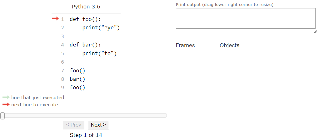
Again, this is very familiar to us based on what we’ve seen so far. So, let’s click the Next > button to step through the first part of the code:
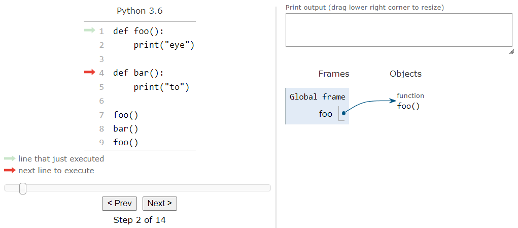
As we can see, the first thing that Python sees is the definition for the foo function. Instead of keeping a separate list of functions, Python Tutor simply adds that function to the global frame just like any variable. The function itself is added to the Objects list, and then there is an arrow, connecting the variable in the global frame to the function in the objects list. In fact, this is exactly how Python handles functions - they are just treated like variables that are pointers to the function objects themselves! So, when we click Next > again, we’ll see it do the same to the bar function as well:
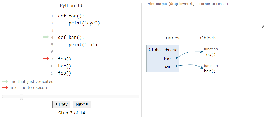
At this point, we are ready to execute the first function call, which will run the foo function. So, when we click the Next > button, we’ll see the arrow jump to the start of that function:
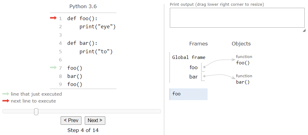
Here, we see Python tutor do something a bit different than in our own code traces - instead of keeping all of the variables in a single box, it creates a new frame to keep track of the variables that are created in the foo function. When we look an example of a function with parameters, we’ll see where this becomes very useful. For now, we can just ignore it and move on by clicking Next > once again:

At this point, the function is ready to print the string value "eye" to the terminal. So, if we click Next > once again, we should see that reflected in the output of Python Tutor:
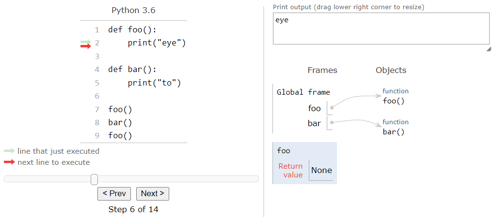
At this point, we’ve reached the end of the foo function. So, Python Tutor will remove the foo frame from the list of frames and it will jump back down to where the function was called from when we click Next >:
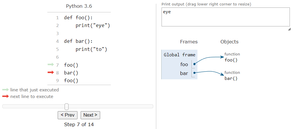
Here, we are back to the main piece of our code, and we’re ready to call the bar function. So, we can click Next > once again:
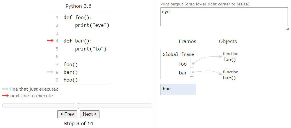
This will jump up to the start of the bar function and create a new frame for storing any variables created by bar. We can click Next > again to enter the function:
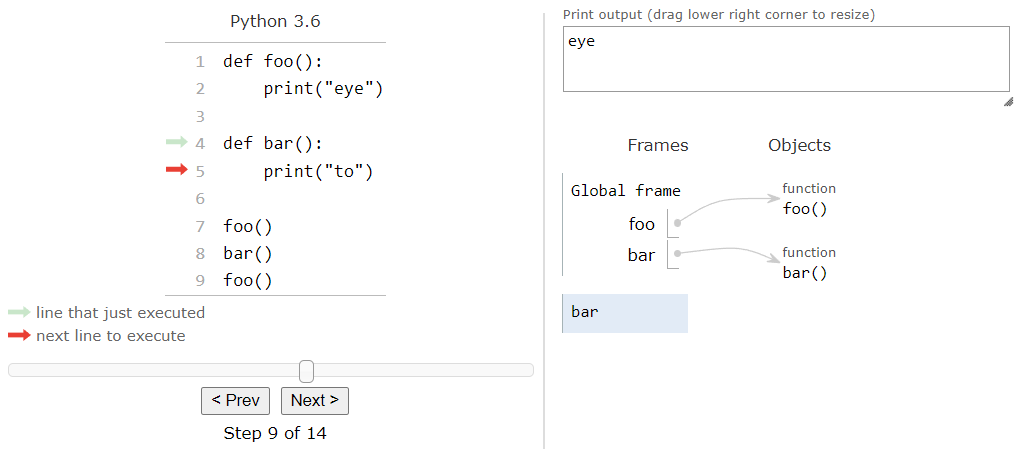
And then click Next > again to print the string value "to" to the output:
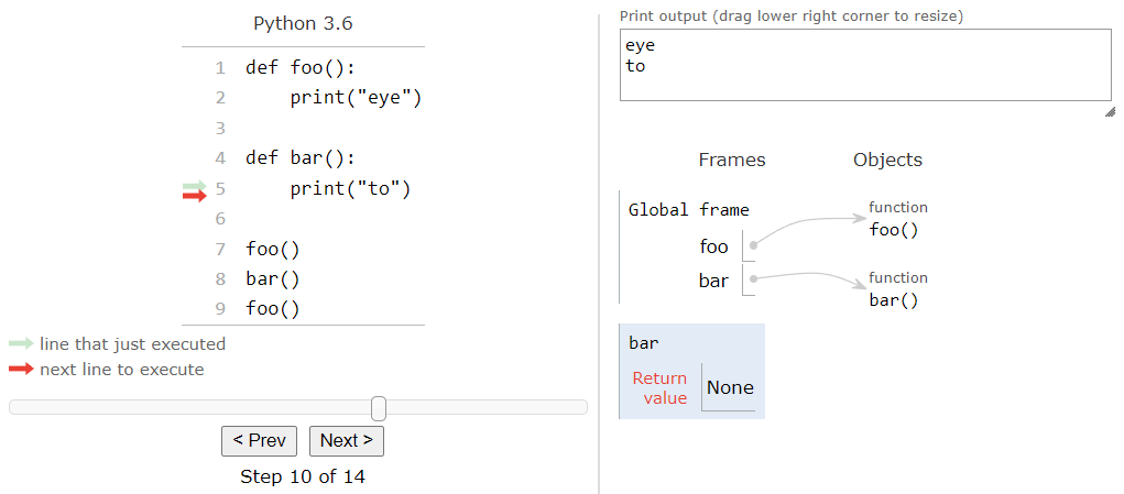
Once again, we are at the end of a function, so when we click Next > once more:
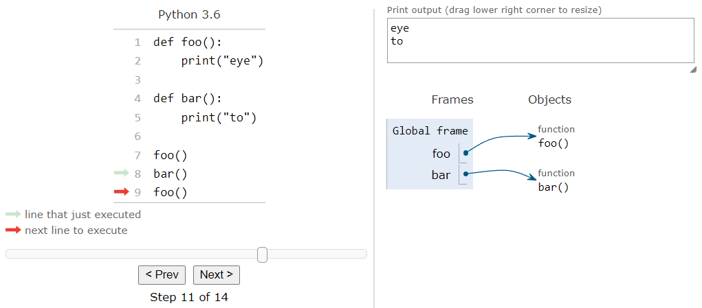
We’ll move back to the main piece of the code, removing the frame for bar. On this line, we see yet another function call, this time to the foo function. Hopefully by this point we can predict what is going to happen, so we can click Next > a few more times to jump to the foo function and execute it. When it is done, we’ll see this output:
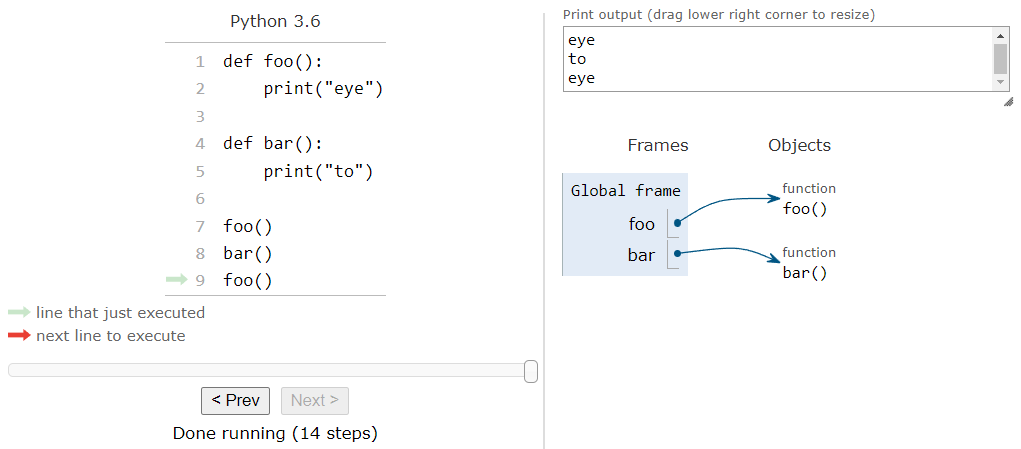
There we go! We’ve successfully traced the execution of a Python program that contains multiple function calls. The full process is shown in this animation:

Using tools like Python Tutor to trace through code is a great way to make sure we understand exactly what our computer is doing when it is running our code.
Let’s review a couple other concepts related to functions in Python. These will closely mirror what we’ve already learned in pseudocode, so we’ll cover them pretty quickly here.
Just like in pseudocode, we can also create a main function in Python. The use of a main function in Python is not required at all - Python is designed as a scripting language, meaning we can write code directly in a Python file without using any functions at all. However, it is generally considered good practice to make sure all code is part of a function, and then we can include a main function as the starting point for any program.
So, we can update the example we saw previously to include a main function by simply placing the three function calls in a new function called main, and then including a call to the main function at the bottom of the program:
def foo():
    print("eye")


def bar():
    print("to")


def main():
    foo()
    bar()
    foo()


main()
From here on out in this course, we’ll follow this convention in our complete Python programs. Specifically:
main as the starting point of the program.main function at the bottom of the program.This will make our Python programs easy to follow, and it will help us later on down the road if we choose to learn another language such as Java or C# that requires a main function.
Functions in Python can also require parameters. To include a parameter in a function, we simply have to include the name of the parameter in the parentheses () at the end of the function definition. Multiple parameters should be separated by commas ,. For example, we can update our hello_world function to include a couple of parameters:
def hello_world(first_name, last_name):
    print("Hello ", end="")
    print(first_name, end=" ")
    print(last_name)
Here, we are defining two parameters, named first_name and last_name, that are used as part of the function. Those parameters can be treated just like any other variable within the function.
Once we have a function that requires parameters, we can call it by including arguments in the parentheses () that are part of the function call. For example, we can call the hello_world procedure above and provide two arguments like this:
hello_world("Willie", "Wildcat")When we run this code, it will place the string value "Willie" in the parameter variable first_name, and the string value "Wildcat" will be placed in the parameter value last_name within the frame for the hello_world function. When the code in hello_world is executed, we should see the following output:
Hello Willie WildcatTo see how this works, let’s work through a full example. Here’s a more complex Python program that includes parameters, arguments, and some other variable expressions:
def flip(first, last):
    temp = first
    first = last
    last = temp
    print(first)
    print(last)


def main():
    first = "Willie"
    last = "Wildcat"
    flip(first, last)
    print(first)
    print(last)


main()
Once again, before reading the full analysis below, take a minute to read through this code and see if you can guess what it does. It can be a bit tricky if you don’t read it carefully and think about what we’ve learned so far.
To trace this example, copy the code into the tutor.py file in the python folder on Codio, or click this Python Tutor
link.
When we begin, our code trace will look like this example:
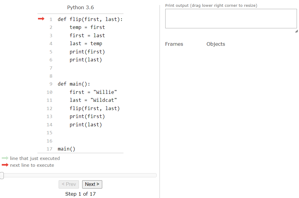
As we expect, the first thing that Python will do is scan through the code and record any functions it finds in the global frame. So, after pressing the Next > button a couple of times, we should reach this point:
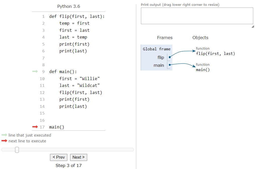
Now we are at a function call for the main function. So, when we click the Next > button:
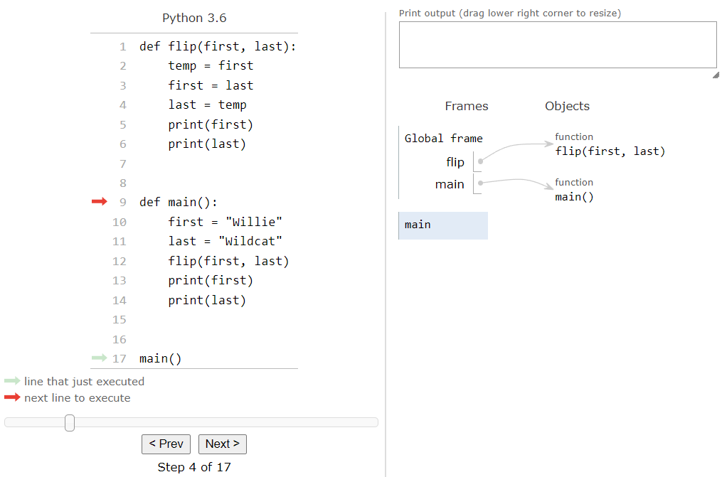
Python tutor will jump to that function’s code, and it will also create a new frame for variables that are created in the main function. The next two lines deal with creating a couple of variables, so we can click the Next > button a couple of times to execute those lines and stop when we reach the next function call:
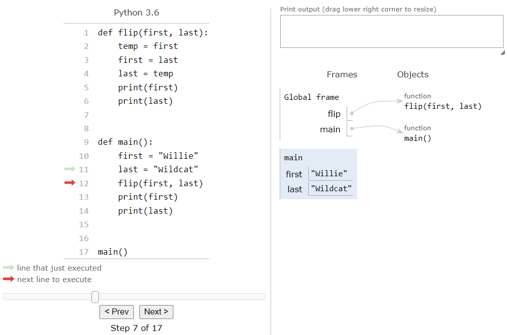
Now we are ready to call the flip function. This function requires two parameters, named first and last. Notice that those parameter names are the same names as the variables that we created in the main function? This is a common practice in programming - sometimes it is simplest to use the same variable names in multiple functions, especially if they are storing the same data. However, it is important to understand that those variables are not related in any way except for the name, as we’ll see in this example. When we click the Next > button to jump to the start of the flip function, we should see the following in our Python tutor trace:
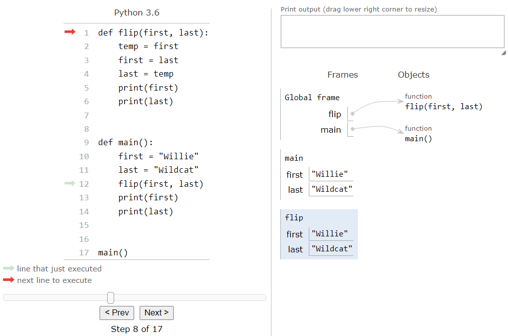
It has now created a frame for the flip function, and copied the values of the two arguments into the appropriate parameter variables. Since we listed the arguments first and last in that order in the function call to flip, a copy of the values from those two variables in main will be stored in the same two variable names in flip. It’s an easy way to make sure the arguments are in the correct order!
The first three lines in the flip function will swap the values in the first and last parameter variables. So, after we’ve executed those three lines, we should now see this setup in our trace:
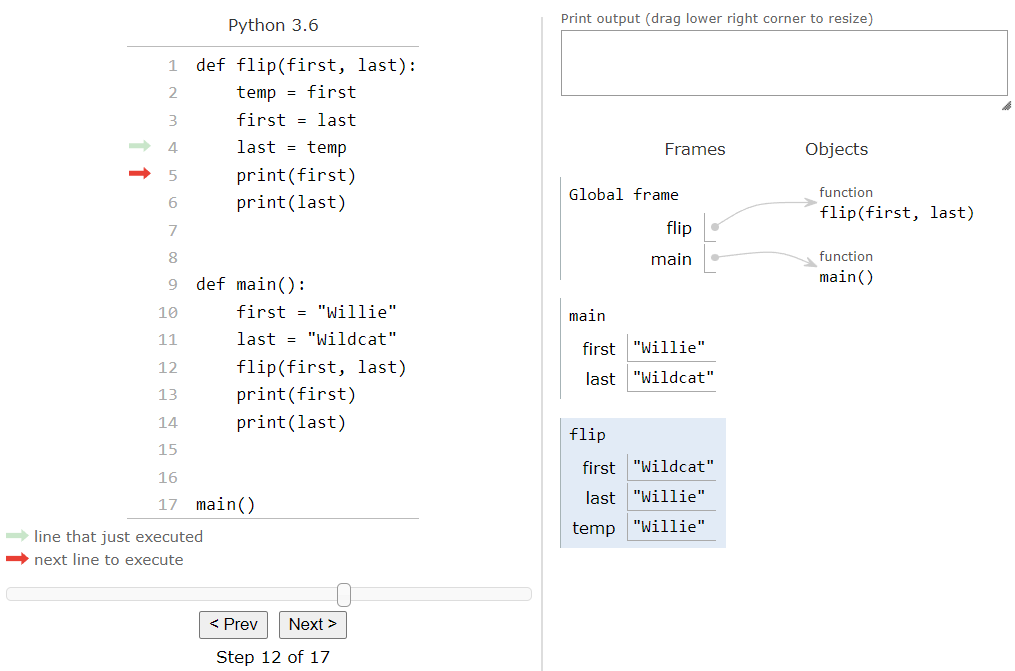
Notice that the values in first and last inside of the flip frame have changed, but the values in the same variables in the main frame have not changed! This is why it is very useful to keep track of variables in frames within a code trace - we can easily tell which variables go with which function, even if they have the same names. So, the next two lines of code in the flip function will simply print out the contents of the first and last parameter variables:
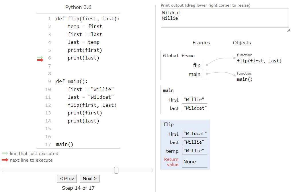
At this point, we’ve reached the end of the flip function, so when we click the Next > button again, we’ll jump back down to where we left off in the main function. At the same time, we’ll remove the flip frame from the list of frames, completely removing the first and last parameter variables used in that function:

Now that we are back in the main function, we can see that the values stored in the first and last variable are unchanged, just like we’d expect. This is important to understand - just because one function uses the same variable names as another function, or that a function’s parameter names match the variable names provided as arguments, they are not related and any changes in the function won’t impact the values outside of the function. So, we can finish the main function by running the last two lines, which will print the current values of first and last to the screen:
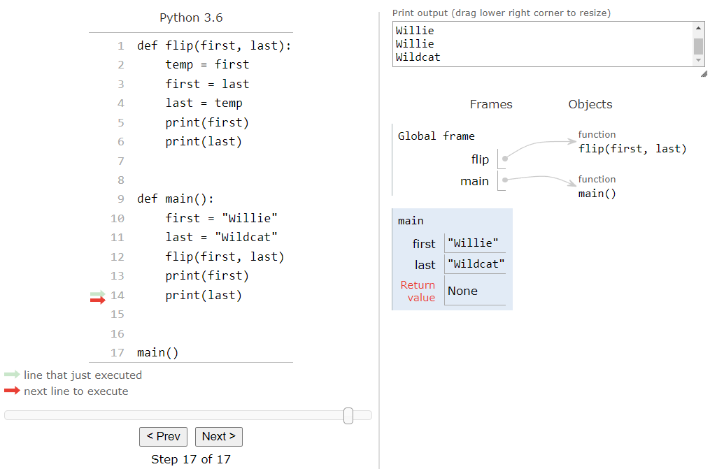
Finally, once the program reaches the end of the main function, it will jump back to the main function call at the bottom of the program. This will remove the main frame from the list of frames. Since there is nothing more to do, the program will end at this point:
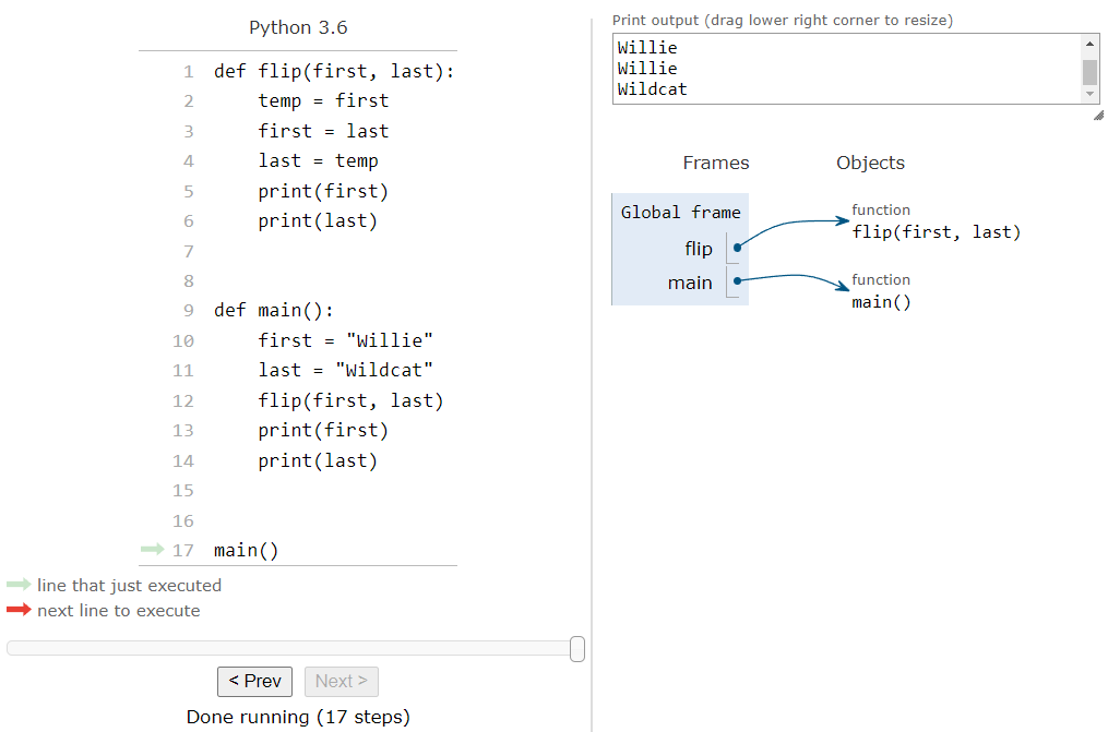
The whole process can be seen in this animation:

There we go! We’ve explored how functions, parameters, and arguments all work in Python. Understanding this process now will make it much easier to write complex programs later on.
A procedure in pseudocode is a piece of code that is given a name, which can then be run by calling it elsewhere in the program.
To create a procedure, we use the following structure:
PROCEDURE procedure_name(parameter1, parameter2)
{
    <block of statements>
}{}. These lines of code are indented to make it clear that they are part of the procedure.To call a procedure, we use the following structure:
procedure_name(argument1, argument2)().A function in Python is a piece of code that is given a name, which can then be run by calling it elsewhere in the program.
To create a function, we use the following structure:
def function_name(parameter1, parameter2):
<block of statements>To call a function, we use the following structure:
function_name(argument1, argument2)().As we’ve seen, procedures in pseudocode and functions in Python are very similar. They allow us to write pieces of code that we can use repeatedly throughout our programs. This makes our programs more organized and modular, and will make it much easier to write more complex programs as we continue to develop our skills.s
Previously, we learned about strings and string values in pseudocode. Recall that a string is just text inside of a set of quotation marks "", such as "Hello World" or "Willie Wildcat". In technical terms, a string is an example of a data type in programming. A data type defines the way a particular value can be stored in a computer. For text values, we use the string data type.
What about numbers? We all know how important numbers can be, especially since we’ve probably spent more time studying mathematics than just about any other subject in school. So, let’s introduce a new data type in pseudocode called the number data type. This data type can store any single number, such as $1$ or $2.3$ or even special numbers like $\pi$ (pi) or $e$ (Euler’s number).
So, to create an expression that evaluates to a numerical value in pseudocode, we can just use the numbers in our code instead of text in quotes. For example, to store the number $7$ in a variable, we’d use the following assignment statement in pseudocode:
num1 <- 7Notice that the numerical value 7 in our code does not have quotation marks around it. This is because we want to treat it like a numerical value instead of a string.
Also, recall from earlier that we cannot use a number as the first symbol in a variable name? This is because numerical values must always start with a number, so we enforce this rule to allow us to tell the difference between numerical values and variable names.
For a number with a decimal in it, such as $1.23$, we can use a similar process:
num2 <- 1.23If we have a value that is less than $1$, we must put a 0 in front of the decimal point, like this:
num3 <- 0.42We can also create negative values by placing the negative symbol - (the same symbol as the minus sign) in front of the numerical value:
num4 <- -4.56Notice that we have to be careful to include a space between the arrow symbol <- in the assignment statement and the negative symbol - for a negative value.
As we can see, creating variables that store numerical values is pretty easy, and it hopefully works exactly like you expect it to work.
Now that we have two different data types, strings and numbers, it might be useful to convert between the two data types. Officially, the AP Pseudocode does not include an explicit way to convert between data types, or any concept of different data types at all. Instead, they just assume that variables can “automagically” convert data as the developer intended, without performing any additional steps.
However, this can get a bit confusing, so we’ll briefly introduce two different procedures in pseudocode that can handle converting data between different types.
To convert any type of data to a number, we can use the NUMBER(expression) procedure. It will evaluate the expression to a value, and then convert that value to a number. Of course, this requires us to make sure that whatever value we get when we evaluate the expression will make sense as a number. Since we aren’t running this on a real computer, we don’t have to worry about any errors or crashes - instead, it will just mean that our program won’t make any sense when we try to run it on our “mental model” of a computer.
Likewise, to convert any data to a string, we can use the STRING(expression) procedure in a similar way. Thankfully, pretty much any value in any data type can be represented as a string in some way, so we don’t have to worry about this procedure causing issues if the expression results in a strange value.
Now that we have the ability to store numerical data in variables in pseudocode, we should also learn how to manipulate that data into something new. To do that, let’s learn about operators. An operator in programming is a special symbol that can be used in an expression to manipulate the data in some way. Most operators are binary operators, which means they perform an operation that uses two values as input and produces a single value as output. In fact, in some programming languages, the operators themselves are implemented as procedures in the language!
An expression containing a binary operator typically follows this format:
<expression> <operator> <expression>As before, the <expression> parts can be any valid expression in the language, and the <operator> part is typically a single symbol, but it can also be a short keyword as well.
Thankfully, these operators should all be very familiar to us from mathematics already, so this is just a quick discussion of how they can be used in programming.
For starters, we can use the plus + and minus - symbols as operators to perform addition and subtraction in pseudocode, just like in math. For example, we can add two variables together to create a third variable as shown in this example:
a <- 5
b <- 7
c <- a + b
DISPLAY(c)
When we run this code on our “mental model” of a computer, we should get this result:
12Likewise, we can subtract two variables using the minus symbol - as shown here:
x <- 24
y <- 10
z <- x - y
DISPLAY(z)
This code should produce this output:
14In pseudocode, we use the asterisk *, sometimes referred to as the star symbol, to multiply two values together. For example, we can find the product of two values as shown in this pseudocode block:
a <- 6
b <- 7
c <- a * b
DISPLAY(c)
When we run this code, we should see the following result displayed to the user:
42Division is performed using the slash / symbol. A great way to think of division in programming is just like a fraction, since it uses the same symbol between the two numbers. For example, if we execute this code:
x <- 27
y <- 3
z <- x / y
DISPLAY(z)
we would see this output:
9What if the division would result in a remainder? In that case, we’ll simply use decimal values in pseudocode so that the result is exactly correct. For example, if we try to divide $19$ by $5$, as in this example:
a <- 19
b <- 5
c <- a / b
DISPLAY(c)
Our “mental model” of a computer would produce the following output:
3.8So, as we can see, all of these operators in pseudocode work exactly like their counterparts in math. Even though we aren’t running our code on an actual computer, we should be easily able to use a simple calculator to help us perform these operations if needed.
There is one other operator that is used commonly in pseudocode - the modulo operator. The modulo operator is used to find the remainder of a division operation. If we think back to math again, we’ve probably learned how to perform long division
when dividing two values. At the end, we might be left with a remainder, or a portion of the first number that is left over after the operation is complete. In many computer programs, that value is very useful, so we have a special operator we can use to find that value. In pseudocode, we use the keyword MOD as the modulo operator.
For example, if we want to find the remainder after dividing $19$ by $5$, we would use the following code:
x <- 19
y <- 5
z <- x MOD y
DISPLAY(z)
When we run this code, we would get the following output:
4This is because the value $5$ will fit into the value $19$ only $3$ times, and then we’ll have the value $4$ left over. Mathematically, we are saying that $19 / 5 = (3 * 5) + 4$. Since $4$ is the leftover portion, it is the resulting value when we use the modulo operator.
In this course, we’ll only worry about how the modulo operator works when applied to positive whole numbers. In practice, it can be applied to any numerical value, including decimal values and negative numbers, but those values are not really useful in most cases. So, to keep things simple, we’ll only use positive whole numbers with this operator.
Finally, just like in mathematics, we must also be aware of the order that these operators are applied, especially if they are combined into a single expression. Thankfully, the same rules we learned in mathematics apply in programming as well. Specifically, operators in pseudocode are applied in this order:
*, / and MOD are resolved second, moving from left to right.+ and - are resolved third, moving from left to right.In most cases, it is best to include parentheses whenever we include multiple operators on the same line, just so the intended interpretation is perfectly clear. However, let’s work through a quick example just to see the order of operations in practice.
Here’s a complex expression in pseudocode that we can try to evaluate:
x <- 8 / 4 + 5 * (3 + 1) - 7 MOD 4Looking at our order of operations, the first step is to handle any expressions inside of parentheses. So, we’ll first start with the expression (3 + 1) and evaluate it to 4.
x <- 8 / 4 + 5 * 4 - 7 MOD 4Then, we’ll go right to left and perform any multiplication, division, and modulo operations. This means we’ll evaluate 8 / 4, 5 * 4 and 7 MOD 4 and replace them with the resulting values:
x <- 2 + 20 - 3Finally, we’ll perform addition and subtraction from left to right. So, we’ll evaluate 2 + 20 first, and then subtract 3 from the result of that operation. At the end, we’ll have this statement:
x <- 19So, we were able to use our knowledge of the order of operations to evaluate that complex expression to a single value, $19$, which will be stored in the variable x.
So far, we’ve only worked with string values in Python. Strings are a very useful data type in programming languages such as Python, but they are very limited in their use. Recall that a data type simply defines how a particular value is stored in a computer. The str data type is used to store string values in Python.
Python supports many different data types for handling various data that we’d like to store and manipulate in our programs. In this lab, we’re going to cover the two basic types used for storing numbers in Python, the int or integer type, and the float or floating-point type.
In mathematics, an integer is a whole number, such as $3$, $-5$, or even $0$. Basically, any positive or negative number that doesn’t include a fractional or decimal portion is a whole number, and therefore it is an integer. In Python, those numbers can be stored in the int data type.
In Python, we can store an integer value in a variable using an assignment statement:
x = 5That statement will store the integer value $5$ in the variable x. Notice that the value $5$ does not have quotation marks around it. This is because we want to store the integer value $5$ and not the string value "5" in the variable. Also, as we learned earlier, this is why we cannot create variable names that begin with a number - since numerical values start with a number, this is how Python can tell the difference between a numerical value and a variable.
Just like in pseudocode, we can also store negative numbers in a variable by placing a negative symbol - in front of the numerical value:
y = -8We’ll need to be careful and make sure that there is a space after the equals sign =, but no space between the negative symbol - and the number after it. Otherwise, the negative symbol could be confused for the minus symbol, which is an operator that we’ll learn about later in this lab.
In Python, there is effectively no maximum size for an integer, so we can store any arbitrarily large whole number (either positive or negative) in an int variable.
The other type of number we can store in Python is a floating-point number. We won’t go into too much detail about floating-point values here, since you’ll learn about them elsewhere in this class. For the purposes of programming, the only thing to know about floating-point numbers is that they are used to represent numbers that include a fractional or decimal portion. In Python, these values are stored in the float data type.
To create a variable that stores a floating-point value in Python, we can use an assignment statement that includes a value with a decimal point, like this:
a = 5.8We can also create negative values using the negative symbol -:
b = -7.987Finally, it is possible to store a whole number in a floating-point value by simply adding a decimal point and a 0 at the end of the value, as in this example:
c = 42.0Later in this lab, we’ll see a couple of situations where that may be useful.
For now, we’re just going to assume that Python can easily handle any reasonable number we want it to store in a float variable, but there are some limits to the size and accuracy of those numbers. To reach these limits, we usually have to be dealing with numbers that have $100$ or more digits, either before or after the decimal place. So, for the purposes of this class, those limits really won’t apply to what we’re doing. You’ll learn about these limits in detail in later programming classes.
One thing that is very useful to know how to do in Python is determining the type of data stored in a variable. Python is very flexible, and we can store any type of data in any variable. In fact, a variable’s data type can even change in Python, which is something that many other programming languages won’t allow. Technically speaking, we would say that Python uses strong typing, which means that each variable has a known data type that we can find, and dynamic typing, meaning that the type of the variable can change while the program is running.
To determine the type of a variable, we can use the type(expression) function in Python. We can simply place any variable or expression in the expression argument, and then it will tell us the type of the value that results from evaluating that expression. Then, we can simply use the print() function to print it to the screen. We won’t use this in our programs themselves, but it can be helpful for debugging purposes or to just better understand what is going on with data types.
Here’s a quick example program showing the type() function in Python:
x = "Hello"
y = 5
z = 6.7
print(type(x))
print(type(y))
print(type(z))
When we execute this code in Python, we should see the following output:
<class 'str'>
<class 'int'>
<class 'float'>
Based on that output, we can assume that the variable x is the str data type for strings, y is the int data type for whole numbers, and z is the float data type for decimal numbers. The type() function is pretty handy!
We can also convert values between the various data types in Python. To do this, there are special functions that match the name of the data types themselves, just like we saw in pseudocode. So, to convert any value to a string, we can use the str() function. Likewise, to convert anything to an integer, we can use the int() function. And finally, to convert anything to a floating-point value, we can use the float() function.
So, we can extend the previous example a bit by showing how we can convert values between different data types:
x = "5.7"
print(x)
print(type(x))
print()
y = float(x)
print(y)
print(type(y))
print()
z = int(y)
print(z)
print(type(z))
When we run this program, we’ll get this output:
5.7
<class 'str'>

5.7
<class 'float'>

5
<class 'int'>
In this program, we’re starting with the string value "5.7" stored in variable x. So, the first two print() statements will print that string value, and show that x is indeed storing a str data type. Then, we’ll use the float() function to convert the string value "5.7" stored in x to the floating-point value $5.7$ and store that in y. The next two print statements will print that value, and show that y is storing a float data type. Notice that the value printed for both variables x and y looks identical, but the data type of each variable is different!
Finally, we can use the int() function to convert the floating-point value $5.7$ to an integer. In math, when we are asked to convert the number $5.7$ to a whole number, our first instinct is probably to just round up to $6$, since that is the closest value. However, in Python, as in most other programming languages, this function will simply truncate the value instead. Truncating a value simply means we take off the end of the value, so to convert $5.7$ to an integer we just remove the decimal portion, and we’re left with the value $5$. So, in the output above, we see that z stores the integer value $5$, and it is the int data type.
Notice that we are careful to say that the int() function will truncate the value, and not that it will round down. This is due to how Python handles negative numbers like $-5.7$. When converting that to an integer, it will also truncate it to $-5$ instead of rounding down to $-6$. So, we use the word truncate as the best way to describe the int() function.
Since we are running our Python programs on a real computer, we have to be a bit careful about how we use these functions. Specifically, if we try to convert a value to a different data type and Python can’t figure out how to do that, we’ll cause an exception to occur. An exception in programming is any error that happens when the computer tries to run our code.
For example, what if we try to convert the string value "5.7" directly to an int data type, as in this example:
a = "5.7"
print(a)
print(type(a))
print()
b = int(a)
print(b)
print(type(b))
When we try to run this code in a file, such as the tutor.py file shown here, we’ll see this output printed on the terminal:
5.7
<class 'str'>

Traceback (most recent call last):
  File "tutor.py", line 5, in <module>
    b = int(a)
ValueError: invalid literal for int() with base 10: '5.7'
Uh oh! That’s not good. In the output, we can see that we’ve caused a ValueError, which is an exception that happens when we try to use a value in an incorrect way. So, we’ll need to carefully look at our code to see if we can find and fix the error.
Thankfully, in the output, it will tell us that the error occurred on line 5 of the file tutor.py, so we can open that file and scroll to that line of code:
b = int(a)This is where the error occurred. There are several ways we can fix it. The easiest would be to simply convert a to a floating-point value using the float() function instead.
Learning how to find and fix these exceptions is a key part of learning how to program. We’ll inevitably run into a few exceptions as we start to build larger and more complex programs. In this course, most exceptions can be easily handled simply by working carefully through the code, but every once in a while we may run into an exception that is truly difficult to solve. That’s one of the important things to remember when learning how to program - it is sometimes much easier to cause an exception than it is to figure out how to fix it, and sometimes you may need to reach out for help to get past a particularly tricky exception. So, don’t be afraid to ask the instructors or TAs for help if you get stuck on an exception. Many times, it’s a great chance for you to learn some new programming skills.
We can also use Python to perform mathematical operations on numerical data using operators. So, let’s briefly review the operators we’ve learned so far, and introduce a couple of new operators that are unique to Python.
Python supports the same mathematical operators that we’ve already seen in pseudocode. The only exception is the the modulo operation is performed using the percent symbol % instead of the MOD keyword. So, here are the symbols we can use in Python and the operations they perform:
+ addition- subtraction* multiplication/ division% moduloHowever, there is one major difference between how these operators work in pseudocode and how they work in Python, and it has to do with the fact that Python includes two numerical data types. To deal with this, we have to define how the operators work when applied to different data types.
The basic rule to remember, if a mathematical operator is applied to two variables of the same data type, the result will also be that data type.
Let’s see what that means in practice. Here’s a quick example in Python using the multiplication operator on two integer values:
x = 5
y = 10
z = x * y
print(z)
print(type(z))
When we run this code, we should see the following output:
50
<class 'int'>
Since both x and y are the int data type, the result of x * y will also be an int value, so the variable z will have that data type, as shown in this example.
However, there is one exception to this rule, which is the division operator /. In Python, the division operator will always return a float value, even if it is a whole number. Here’s an example that demonstrates that:
a = 9
b = 3
c = 4
x = a / b
print(x)
print(type(x))
print()
y = a / c
print(y)
print(type(y))
When we run this program, we’ll see the following output:
3.0
<class 'float'>

2.25
<class 'float'>
So, as we can see, even though we are dividing two int values, we’ll get a float value as a result each time we use the division operator.
Following the rule above, if we perform a mathematical operation between two float values, the resulting value will always be a float as well:
a = 2.5
b = 4.5
c = a + b
print(c)
print(type(c))
Running this code will produce this output:
7.0
<class 'float'>
So, even though the result is a whole number, the value that is stored is the float data type.
The other rule to remember is anytime an operation involves a float value and an int value, the result will be a float. So, if there are mixed types, Python will default to the float data type.
This can be seen in the following example:
a = 5
b = 2.0
c = a - b
print(c)
print(type(c))
When this code is executed, the output should look like this:
3.0
<class 'float'>
Once again, even though the result is a whole number, because the variable b is a float value, the entire result will also be a float value.
In Python, we can also introduce two new operators:
** exponentiation (power)// integer divisionFirst, the double star ** operator is used to represent the exponentiation operation, sometimes referred to the power operator. In Python, the expression 2 ** 3 would be written mathematically as $2^3$, which is the operation of taking $2$ to the power of $3$, or multiplying $2$ by itself $3$ times. This operator follows the rules listed above for determining what type of data is the result of the operation.
Here’s a quick example of using the ** operator in code:
x = 5 ** 3
print(x)
print(type(x))
When this code is run, we see the following output:
125
<class 'int'>
The integer division operator, represented by two forward slashes //, is used to perform division that truncates the result to an integer. However, it still follows the rules for determining the data type of the result as listed above, so if either of the values in the operation is a float value, it will return a float, even though the result is an integer.
Let’s look at an example with that operator in code:
a = 17.5 // 4.5
print(a)
print(type(a))
As we expect, when we run this program, we’ll get the following output:
3.0
<class 'float'>
So, we see that this operator will return a float value, even though it is truncating the result to an integer, simply because the input values contained a float.
Learning the data types that are returned by a mathematical operator can be tricky, but most programmers slowly develop an intuition of how each operator works and what to expect. So, don’t worry too much if this is confusing right now, since it will become much clearer with practice! Also, don’t forget that we can always create a simple test program like the examples shown above to confirm the result for any operation.
Let’s quickly review the order of operations in Python. Thankfully, this is very similar to what we’ve already seen in pseudocode and in mathematics - we just have to add the two new operators:
** is resolved second, moving from left to right*, /, // and % are resolved third, moving from left to right.+ and - are resolved fourth, moving from left to right.Of course, this means that there are now 4 operators that all fit in the “multiplication and division” portion, so we have to carefully make sure they are all taken care of in the correct way. As we learned before it is always best to add extra parentheses to any expression to make the intent very clear instead of relying on the order of operations.
In this lab, we covered several major important topics. Let’s quickly review them.
STRING(expression) to convert an expression to a string if possible.NUMBER(expression) to convert an expression to a number if possible.+ Addition- Subtraction* Multiplication/ DivisionMOD Modulo (the remainder of division)str data type stores text (strings). Use str(expression) to convert an expression to a string if possible.int data type stores whole numbers (integers). Use int(expression) to convert an expression to an integer if possible.float data type stored decimal numbers (floating-point). Use float(expression) to convert an expression to a floating-point value, if possible.+ Addition- Subtraction* Multiplication** Exponentiation (Power)/ Division// Integer Division% Modulo (the remainder of division)So far, we’ve mainly focused on writing programs that can store and manipulate data, but the data itself has always been included in the code itself. While that approach is great for learning the basics, real programs often need to receive data as input from the user. This allows programs to truly be interactive and perform work based on what the user needs. So, let’s introduce a new expression in pseudocode that allows our programs to receive input from the user.
We can use the INPUT() expression in pseudocode to get input from the user. It works just like a procedure, similar to DISPLAY(), but it doesn’t require any parameters. Instead, when evaluated the INPUT() expression will simply result in whatever input value is provided from the user. So, we can use this in an assignment statement to store that value in a variable.
The INPUT() expression can be a bit confusing to work with in pseudocode, since we can only run these programs on our “mental model” of a computer. There isn’t any user interface, and we are acting both as the computer and as the user in most cases. However, this allows us to build and reason about programs that require input from the user, which is a useful skill to develop. As we continue to learn more about a real programming language, we’ll see that this same skill applies there as well.
Let’s look at a quick example of using the INPUT() expression in pseudocode:
DISPLAY("Enter your name: ")
name <- INPUT()
DISPLAY("Hello ")
DISPLAY(name)
As we work through this program, we see the second line requires input from the user. So, it is not longer enough to simply read the code and process what it does - we must also consider what the user inputs as well. For this example, let’s assume the user inputs Willie Wildcat when prompted. In that case, the output should look like this:
Enter your name: Willie Wildcat
Hello Willie Wildcat
In this example, we store the user’s input in a variable named name, and then we print the value of the name variable using a DISPLAY() statement. By default, the INPUT() expression will result in a string value, so it can accept just about any text that the user could provide.
What if we want the user to input a number instead? Traditionally, the AP CSP Pseudocode
would just handle this automatically by converting the data to whatever type is needed or makes the most sense. In this course, however, we’re going to explicitly convert data between types. So, we can use the NUMBER() procedure to make that conversion.
Let’s look at an example:
DISPLAY("Enter a number: ")
text <- INPUT()
number <- NUMBER(text)
square <- number * number
DISPLAY("The square of your input is ")
DISPLAY(square)
Let’s quickly trace this program to understand how it works! We’ll set up our code trace like always, as shown below:

The first line will simply print a prompt to the user for input, so we’ll add that to the output section and move to the next line:

Here, we are asking the user for input. On a real computer, the program would pause with a blinking cursor, allowing the user to enter input. In our code trace, we’ll show the user’s input as white text against a black background. So, if the user enters the text 6, it would look like this in our code trace:
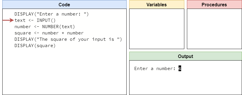
The INPUT() expression will give us that value, which we can store in the text variable as shown in this step:
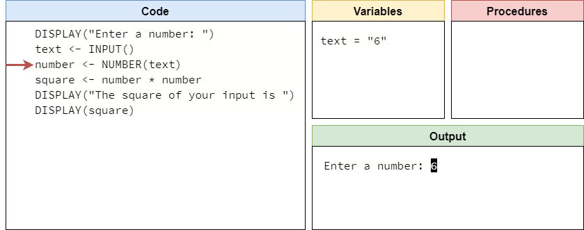
The next line will use the NUMBER() procedure to convert the text value "6" to the numerical value $6$ and store that in the new number variable:
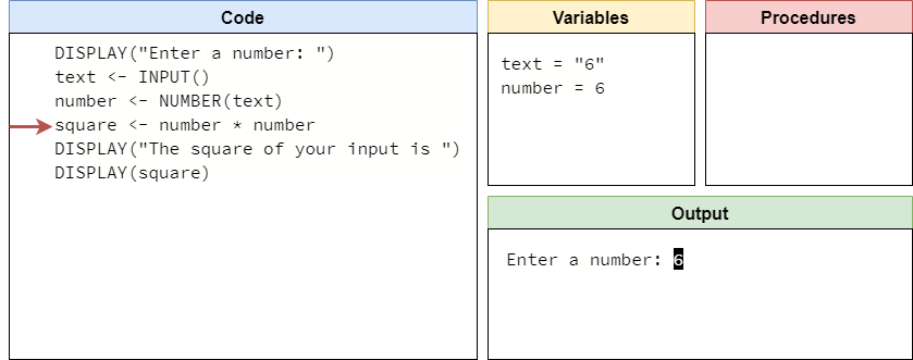
Notice that the value $6$ in the number variable does not have quotes around it. In our code traces, just like anywhere else, we’ll be careful to make sure that string values are surrounded by quotation marks, and numerical values are not.
On the next line, we’ll compute the square of the input by multiplying it by itself, and storing that result in the square variable:
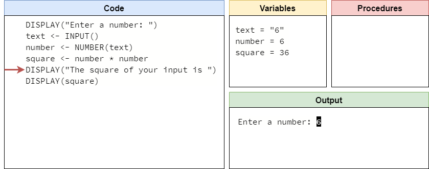
Finally, the last two lines of the program will display output to the user, including the new square value. We’ll start this output on the next line, since user input usually ends with the user pressing the ENTER key to denote the end of the input, which results in a newline character that is part of what is shown on the screen:
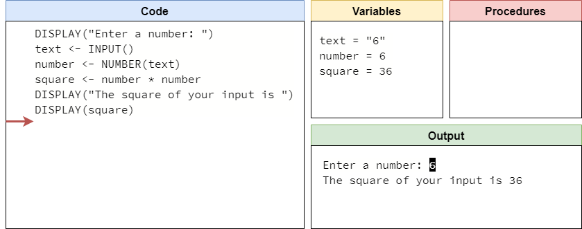
The full process can be seen in this animation:
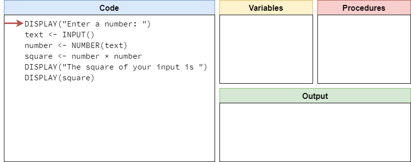
This example shows us quite a bit about how we can use the INPUT() expression in our pseudocode to build programs that are interactive and allow the user to input data for our programs to store and manipulate.
So far we’ve only looked at operators that can be used on two numeric values, but there are also a few operations we can perform on strings as well. Let’s look at one important operator that is commonly used with strings - the concatenation operator. In pseudocode, like most other programming languages, we’ll use the plus symbol + to represent the concatenation operator.
The term concatenate may be a new term, since it isn’t used very often outside of programming. To concatenate two items, we are simply linking two items together, one after the other. When applied to strings, we can use the concatenate operator to combine two strings into a single string.
Let’s look at an example:
one <- "Hello"
two <- "World"
message <- one + " " + two
DISPLAY(message)
In this code, we begin with the strings "Hello" and "World" stored in two separate variables, one and two. Then, we create a new variable message, which contains the values of one and two concatenated together, with a space in between. Since one and two are strings instead of numbers, we know the + symbol represents the concatenate operation, instead of addition.
When we run this program on our “mental model” of a computer, we should see this output:
Hello WorldAs we can see, the concatenate operator is a way we can build complex strings from various parts.
Because the concatenate operator works with strings, we have to add a couple of rules to how our pseudocode language handles data types to deal with this. Here are the most important rules to follow:
+ operator are strings, then the + operator is treated like a concatenation. If both sides are numbers, then it is treated like addition. The + operator cannot be applied to a string and a number.This may seem a bit confusing to anyone who has experience with programming, since many programming languages allow us to use the + operator between strings and numbers without any issues. However, in this case we’re going to stick closely with what is allowed in Python, so these are the rules we’ll follow in pseudocode.
Getting data from the user is one way we can store data in our programs. What if we want to create a procedure that produces a new data value? We can do that using a special statement called the return statement.
In a procedure, we can choose any expression to be the result of calling the procedure, which will allow us to use the procedure as part of an expression instead of a statement. To really understand how this works, let’s see it in action! Here’s an example of a complete pseudocode program with a procedure that returns a value:
PROCEDURE mult_mod(value, multiply, modulo)
{
    value <- value * multiply
    value <- value MOD modulo
    RETURN(value)
}

PROCEDURE main()
{
    DISPLAY("Enter a value: ")
    text <- INPUT()
    value <- NUMBER(text)
    answer <- mult_mod(value, 5, 3)
    DISPLAY(answer)
}

main()
In the mult_mod() procedure, we see that the last line of code is RETURN(value). This line will end the procedure, and it will use the current value stored in the value variable as the return value from the procedure. Then, in the main() procedure, we see that the procedure call for mult_mod() is actually part of an assignment statement answer <- mult_mod(value, 5, 3). So, when the mult_mod() procedure is called, it will perform its work and then produce a return value, which can then be stored in the answer variable in the main() procedure. In effect, we can now use a procedure call to compute a value, which is a very useful thing in our programs. Let’s work through a code trace using this code to see how it works.
Like always, we’ll start with the usual setup for our code trace as shown below.
The first few steps will simply find the procedures declared in the code. Once we reach the call to the main() procedure at the bottom, we should be at this state:
So, we’ll enter the main() procedure. Here, we print a prompt to the user, and then accept input using the INPUT() expression:
In this example, let’s assume the user inputs the number $7$ as input. So, we’ll update our code trace to show that string value being stored in the text variable:
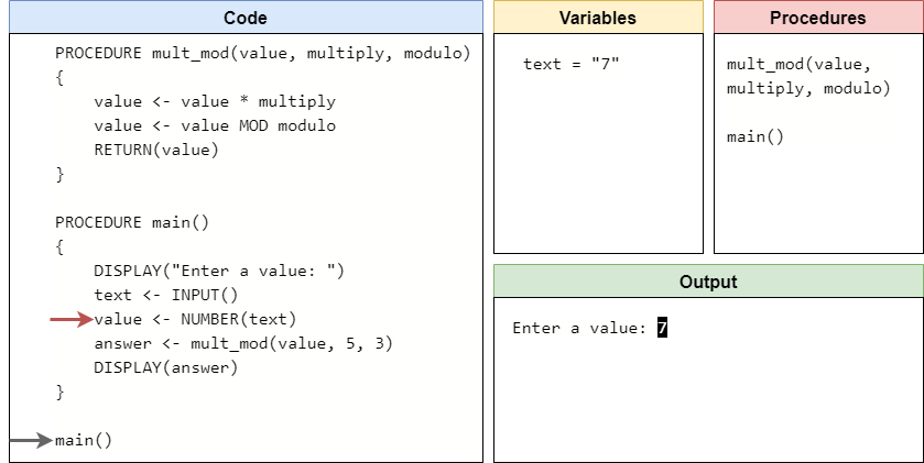
Next, we’ll need to convert that string value to a numerical value using the NUMBER() procedure, storing that result in the value variable:
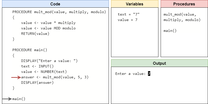
At this point, we are ready to call the mult_mod() procedure. So, we’ll jump up to the first line of that procedure, and create a new set of variables that represent all of the parameters of the mult_mod() procedure, with values matching the arguments provided in the procedure call:
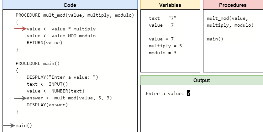
The first two steps of the mult_mod() procedure will multiply the value parameter by the multiply parameter, then find the modulo of that result and the modulo parameter. As it does so, it updates the value stored in the value variable. Once it is done, value should store the value $2$:

Now we’ve reached the RETURN() statement. This statement will end the mult_mod() procedure, so for this example it is the last line of code. Inside of the RETURN() statement, we are choosing to return the value stored in the value variable. So, in our variables list, we’ll remove all of the variables from the mult_mod() procedure, but we’ll place a special variable there showing the value that is being returned from the procedure. In our code trace, we’ll just call that the RETURN variable:
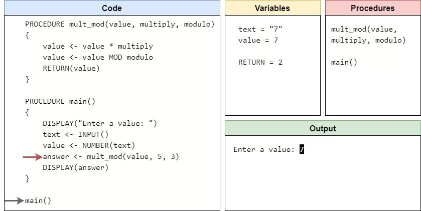
Now, back in the main() procedure, we can deal with the assignment statement on the current line. Here, we will take the value returned from the mult_mod() procedure, which we see as the RETURN variable, and store that value in the answer variable in main. Once we’ve done that, our code trace will look like this:

Notice that the RETURN variable disappears once we’ve passed that line. The RETURN value is only used immediately after the procedure is called, to help evaluate the expression that it is a part of. Once that is done, the value is no longer needed.
Finally, we can complete the program by printing the answer to the output:
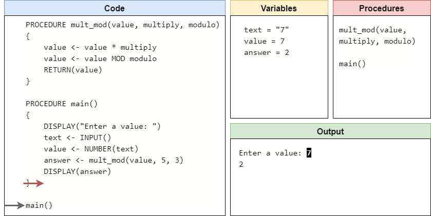
We’ll reach the end of the main() procedure, and once we’ve moved back to the outer level of the code, we’ll see that there is no more work to be done. The full trace is shown in this animation:
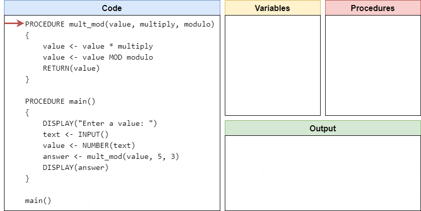
Returning values from a procedure is a really useful tool in programming. It allows us to create procedures that can perform a complex calculation for us, and then we can use those procedures in other expressions to perform even more complex calculations. It is all about finding ways to simplify our programs by creating small, repeatable pieces of code for each task.
Previously, we worked through this simple example pseudocode program:
DISPLAY("Enter a number: ")
text <- INPUT()
number <- NUMBER(text)
square <- number * number
DISPLAY("The square of your input is ")
DISPLAY(square)
However, we can greatly shorten this program’s code using a couple of programming features that we have not covered yet. Let’s look at how we can do that.
The single biggest thing to understand about expressions in programming is that we can usually combine them in a variety of different ways.
For example, this program receives input from the user using the INPUT() expression, and then on a separate line of code it uses the NUMBER() procedure to convert it to a number and store it in a variable. However, since the NUMBER() procedure allows us to use any expression as an argument, we can combine those two lines:
DISPLAY("Enter a number: ")
number <- NUMBER(INPUT())
square <- number * number
DISPLAY("The square of your input is ")
DISPLAY(square)
Yup, that’s right! Because INPUT() is essentially a procedure that returns a value, we can directly use that returned value as an argument to the NUMBER() procedure, without ever storing it in a variable. Our “mental model” of a computer will call the procedure inside the parentheses first, just like we’d expect, and then once it returns a value it will use that value to call the other procedure.
We can combine the last two lines of code in a similar way. We’ve already seen how to combine strings using the concatenation operator, so as long as we convert the value in square to a string it will work:
DISPLAY("Enter a number: ")
number <- NUMBER(INPUT())
square <- number * number
DISPLAY("The square of your input is " + STRING(square))
So, we’ll just place the square variable in the STRING() procedure to convert it to a string value, and then we can concatenate that value onto the end of the other string and display it in a single line.
Finally, we can even perform operations directly inside of procedure calls. So, we can combine the last two lines in this new example, preventing us from even needing the square variable at all:
DISPLAY("Enter a number: ")
number <- NUMBER(INPUT())
DISPLAY("The square of your input is " + STRING(number * number))
Our computer knows to resolve any expressions used as an argument in a procedure before calling the procedure, so this will work exactly like we’d expect it to. So, we’ve taken a program with 6 lines of code and reduced it to just 3 lines of code, and removed 2 of the 3 variables it uses in the process.
The real question is: which of these two examples is best? That is, which one is the preferred coding style to learn? The answer is that it really depends - both have their merits, and functionally they will work nearly identically on most modern computers and programming languages.
It really is a question of style - is it better to have more lines of code and variables, clearly spelling out what each step of the process is, or is it better to have shorter programs with more complex lines of code but maybe fewer variables? For beginning programmers, it is usually recommended to follow the first style, using as many variables as needed and focusing on short, concise lines of code over large, complex statements.
However, as we become more accustomed to programming, we’ll find that many times it is easier to read and understand complex statements, and our code can be written in a way that better reflects what it is actually doing.
This is very similar to learning how to read, write, and speak in a new language. We must start with short, concise sentences, and slowly build up our knowledge of more complex statements and grammar rules until we become a fluent speaker.
Overall, the best advice to follow is to make your code readable to both yourself and anyone else who may have to read and maintain the code. As long as it is clear what the code is doing based on what it says, it is probably a good style to follow. As we continue to learn more, we’ll slowly refine our coding style to be one that is easy to follow and understand for everyone.
The Python programs we’ve written up to this point are very static - each time we run the program, it will perform the same exact operations. Since we’re running these programs on a real computer, it might be helpful to build programs that can read and respond to input from the user, making them much more useful overall. Python includes many different ways to handle user input, but in this lab we’ll just focus on the simple input() function.
The input() function is used to display a prompt the user and then record input. It works very similarly to the INPUT() expression we’ve already seen in pseudocode, but in Python we can display the prompt to the user directly in the input() function itself.
Let’s look at a quick example:
name = input("Enter your name: ")
print("Hello ", end="")
print(name)
Here, we see that the input() function actually accepts a message as an argument, which will be displayed to the user. After the message is printed, the user will be given a cursor to enter text immediately after it. Once the user presses the ENTER key, the input() function will read the input that was entered and store it as a string value or str data type in the name variable.
For example, if the user inputs Willie Wildcat at the prompt, this program’s output will look like this:
Enter your name: Willie Wildcat
Hello Willie Wildcat
We can see this even more clearly in the terminal. When we first run the program, we’ll see the prompt "Enter your name:" printed, followed by a cursor prompting the user to enter something:

Once the user types the input and presses ENTER, the rest of the program will run:
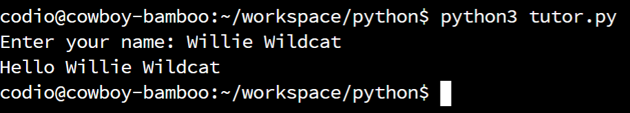
Now we see the cursor is at the next command prompt, ready to run another program.
Of course, we can also read numerical input in Python using the input() function. To do this, we must simply use either the int() or float() function to convert the input received as a string to the correct data type.
Here’s a quick example program that requires two inputs for the price and quantity of an item being purchased:
text_one = input("Enter the price of one item: ")
price = float(text_one)
text_two = input("Enter the quantity of items: ")
quantity = int(text_two)
cost = price * quantity
print("The total cost is $", end="")
print(cost)
If the user wishes to purchase $3$ items at the price of $2.75$ per item, then the program’s output would look like this:
Enter the price of one item: 2.75
Enter the quantity of items: 3
The total cost is $8.25
In the program, we simply read each input from the user as a string value, then use the appropriate conversion function to convert it to the correct data type. For numbers including a decimal point, we use float(), but for whole numbers we use the int() function.
This works well if the user enters values that make sense. But, what if the user wishes to purchase a fraction of an item? Will this program work? Unfortunately, if the user enters a value with a decimal point for the second input, it can no longer be converted to an integer and we’ll get an error:
Enter the price of one item: 2.75
Enter the quantity of items: 3.5
Traceback (most recent call last):
  File "tutor.py", line 4, in <module>
    quantity = int(text_two)
ValueError: invalid literal for int() with base 10: '3.5'
For right now, there’s not much we can do about that error other than write programs that clearly tell the user what type of data is expected, but later we’ll learn how to handle errors like this and prompt the user for input again.
Python also includes an operator that can be used to concatenate two strings together. Just like in pseudocode, we can use the plus symbol + between two strings to concatenate them together into a single string, making it much simpler to build more complex strings and outputs.
A simple example is shown below:
first = "Hello"
second = "World"
print(first + second)
When executed, this code will display this output:
Hello WorldAs we can see, using the + operator in Python to concatenate two strings together is a quick and easy way to simplify our print statements.
Just like in pseudocode, Python also requires both sides of the + operator to be strings in order for concatenation to work. So, if we want to concatenate a string with a numeric value, we’ll have to convert it to a string using the special str() function. Here’s an example:
text = "Your total is $"
value = 2.75
print(text + str(value))
When we run this program, we’ll receive the following output:
Your total is $2.75However, if we forget to convert the value variable to a string, as in this example:
text = "Your total is $"
value = 2.75
print(text + value)
we’ll receive an error instead:
Traceback (most recent call last):
  File "tutor.py", line 3, in <module>
    print(text + value)
TypeError: must be str, not float
So, we’ll have to be careful and make sure that we convert all of our numbers to strings before trying to concatenate them together. Of course, if both sides of the + operator are numbers, then it will perform addition instead of concatenation!
Python also includes another method of building strings, and that is the format() method. The format() method allows us to put placeholders in strings that are later replaced with values from variables, effectively creating a way to build “templates” that can be used throughout our program.
The easiest way to see how this works is looking at a few examples. Let’s start with a simple one:
name = input("Enter your name: ")
print("Hello {}".format(name))
If the user inputs "Willie Wildcat" when prompted, then this code will produce this output:
Enter your name: Willie Wildcat
Hello Willie Wildcat
There are many important parts to this example, so let’s look at each one individually. First, in the print() statement, we see the string "Hello {}". This is an example of a template string, which includes a set of curly braces {} as placeholders for data to be inserted. Each template string can have unlimited sets of curly braces, and each one will be given a different piece of data from the format() method.
Then, we see a period ., followed by the format() method. Notice that the format method is directly attached to the template string by a period - this is because it is actually a method that operates on the template string object itself. This is a key concept in object-oriented programming, which we won’t cover in detail right now, but we’ll definitely see it come up later as we learn more about programming. This is also why we are referring to format() as a method instead of a function, since it is directly attached to another object.
When executed, the format method will replace the placeholders in the string with the values provided as arguments, working from left to right. The first argument will replace the first placeholder, and so on, until all placeholders are replaced and the arguments are all used.
The format() method itself can have unlimited arguments. Each argument corresponds with one of the placeholders in the template string. So, if there are two placeholders, there should also be two arguments.
The Python format() method can do many powerful things, such as place the same argument in multiple placeholders, and each placeholder can define how a value should be presented to the user, among many other features. For right now, we’ll just use simple, empty placeholders in our template strings. Likewise, we’ll just deal with the situation where each placeholder matches to exactly one argument to the format() method.
The most powerful use of the string format() method is to insert numerical values directly into strings without having to convert each value directly to the str data type - the format() method handles that conversion for us.
For example, we can update our previous program to use the string format() method to display the output in a single print() statement, and we can also add additional information with ease:
text_one = input("Enter the price of one item: ")
price = float(text_one)
text_two = input("Enter the quantity of items: ")
quantity = int(text_two)
cost = price * quantity
print("{} items at ${} each is ${} total".format(quantity, price, cost))
When we execute this program, we’ll see output that looks like this:
Enter the price of one item: 2.75
Enter the quantity of items: 3
3 items at $2.75 each is $8.25 total
This example shows how easy it is to build complex output strings using a simple template string and the string .format() method.
Python functions are also capable of returning a value, just like we’ve seen in pseudocode. In Python, we use the return keyword, instead of a RETURN() statement, but the concept is the same.
Let’s look at a quick example of a full Python program that includes a function that returns a value:
def square_sum(one, two):
    one = one * one
    two = two * two
    total = one + two
    return total


def main():
    text_one = input("Enter the first number: ")
    one = int(text_one)
    text_two = input("Enter the second number: ")
    two = int(text_two)
    total = square_sum(one, two)
    print("The sum of squares of {} and {} is {}".format(one, two, total))


main()
To truly understand how this program works, let’s use Python Tutor to explore it step by step. Like before, copy the code into the tutor.py file in the python folder on Codio, or click this Python Tutor
link.
At the start, our Python Tutor trace will look like this:
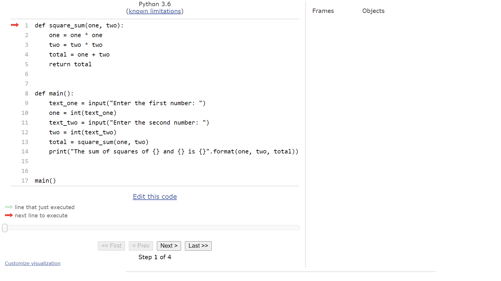
The first few steps are pretty straightforward, since Python will simply move through the code and record all of the functions it finds. Once we reach the call to the main() function at the bottom, we’ll be at this state:
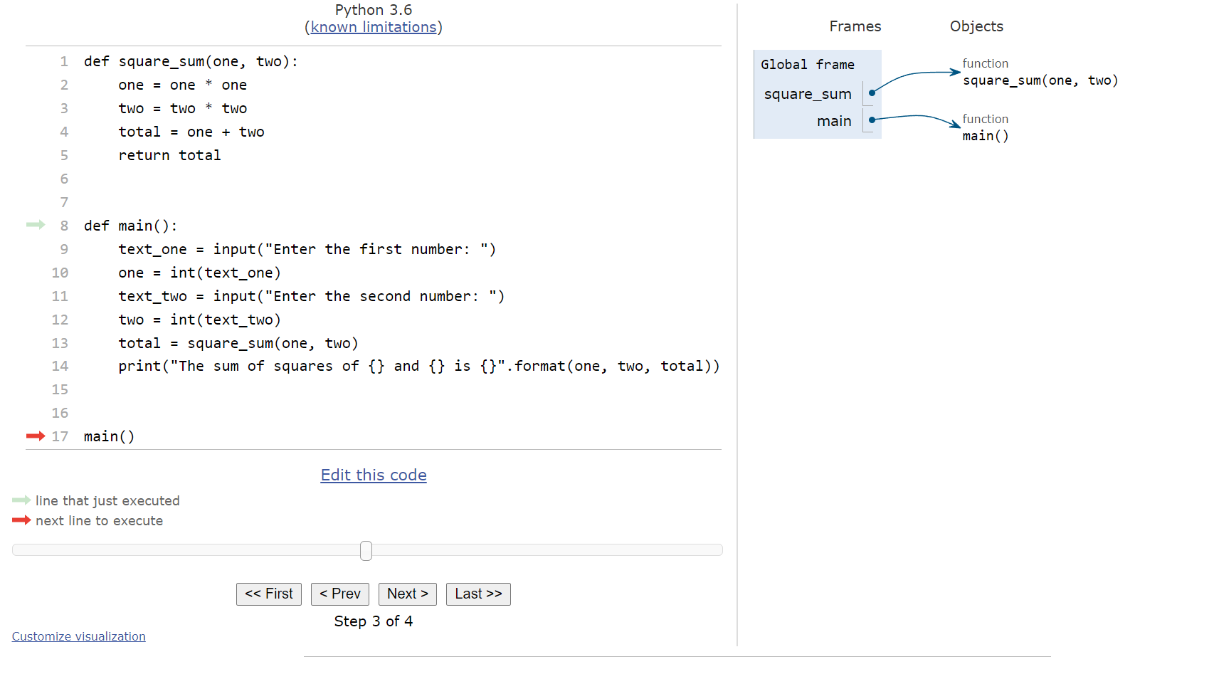
So, we’ll enter the main() function and start executing the code it contains. The first line is an input() expression, so Python will prompt the user for input. In Python Tutor, this will open a box at the bottom where we can enter the input, as shown below:
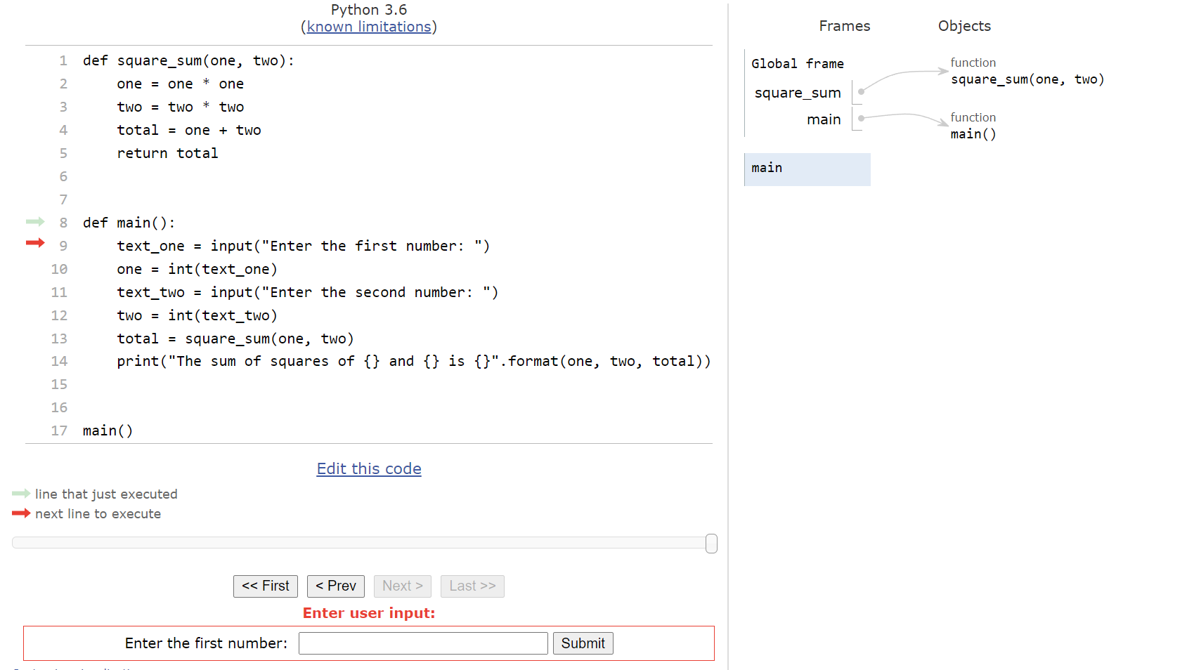
Let’s assume that the user would enter 2 for this input. So, we can type that into the box and press ENTER or click submit. Python tutor will refresh the page to accept the input, and then we’ll be at this setup:
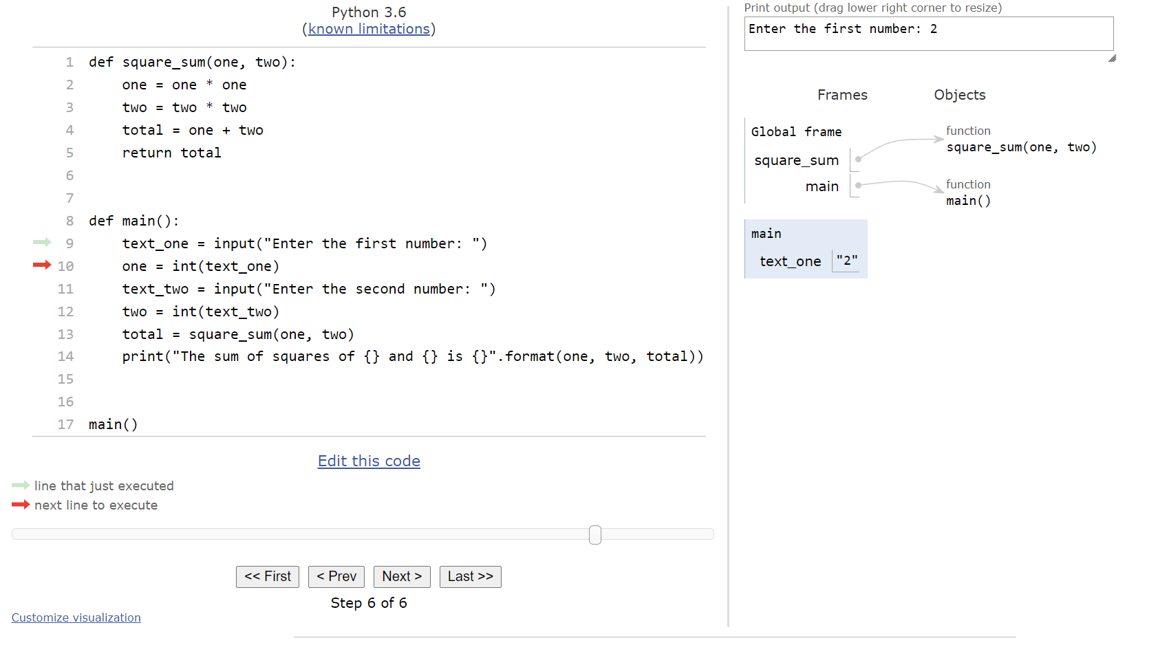
Next, we’ll convert the string value "2" that is currently stored in the text_one variable to an integer using the int() function and store it in the variable one. On the next line, it will ask for input once again:
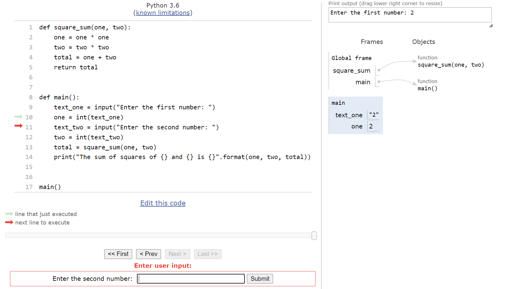
In this case, we’ll assume the user is inputting 3, and then we’ll store it and convert it to an integer stored in the variable two:
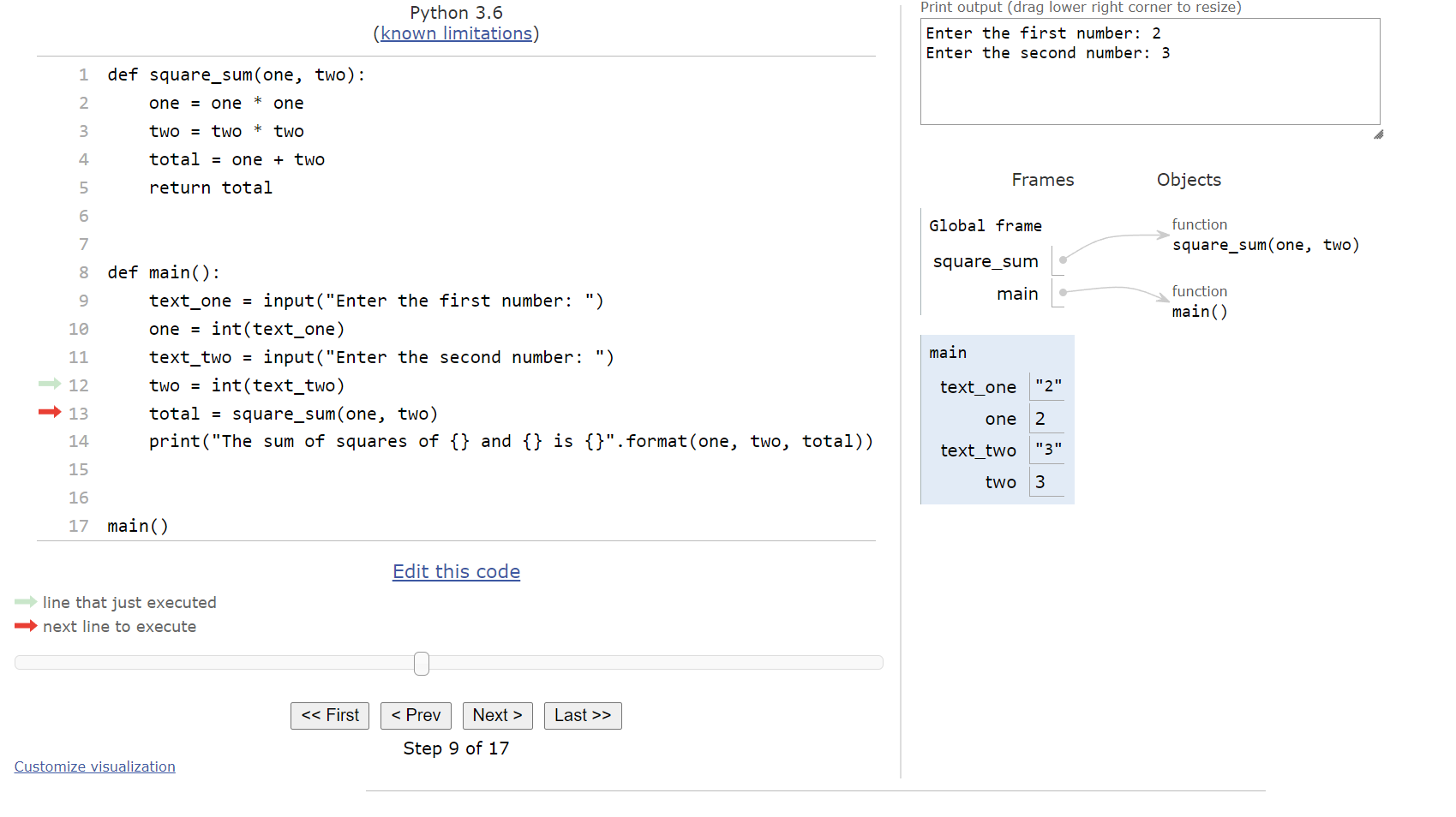
At this point, we’re ready to call the square_sum() function. So, Python Tutor will find the arguments for the function call and prepare to store them in the parameter variables of the function. When we click next, we’ll see this setup in our window:
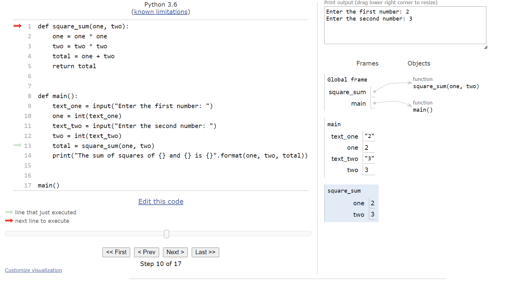
Recall that Python Tutor will create a new frame for the square_sum() function in the frames area and store the variables from that function there. This will become important later when we reach the end of the function. Inside of the square_sum() function, we just perform a few mathematical operations, culminating with the total variable storing the sum of the squares of the two arguments, as shown here:
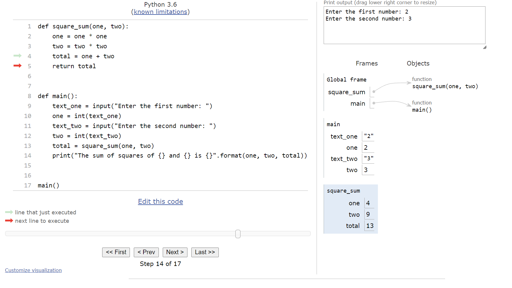
At this point, we’ve reached the return statement at the end of the square_sum() function. When we click next on Python Tutor, we’ll see something new appear:
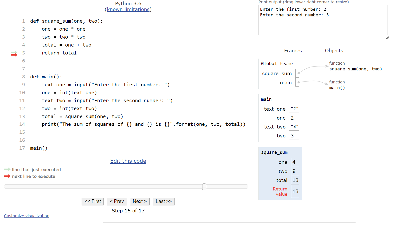
When Python reaches the end of a function, it will record the return value in the function’s frame before leaving the function. This value is what is given back to the main() function. So, when we click next again, we’ll see this state:
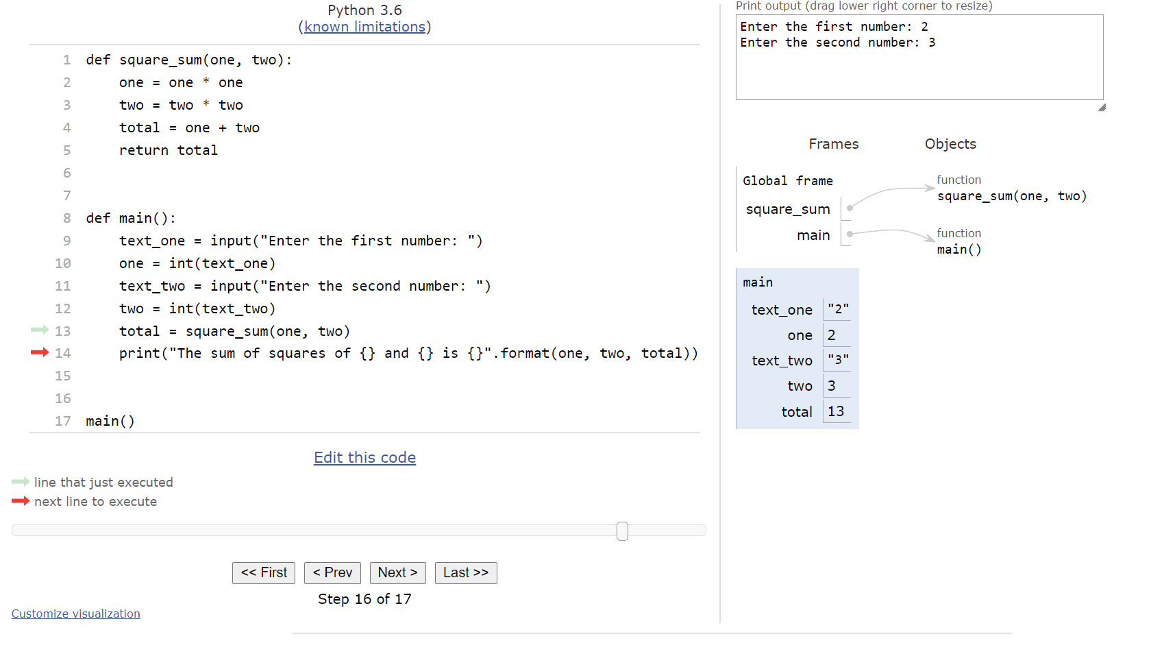
We’re back in the main() function, and now we can see that the new total variable stores the value $13$, which was the returned value from the square_sum() function. So, on this last line, we’ll see that the program will create an output statement using a template string and the string format() method, and it will display output to the user:
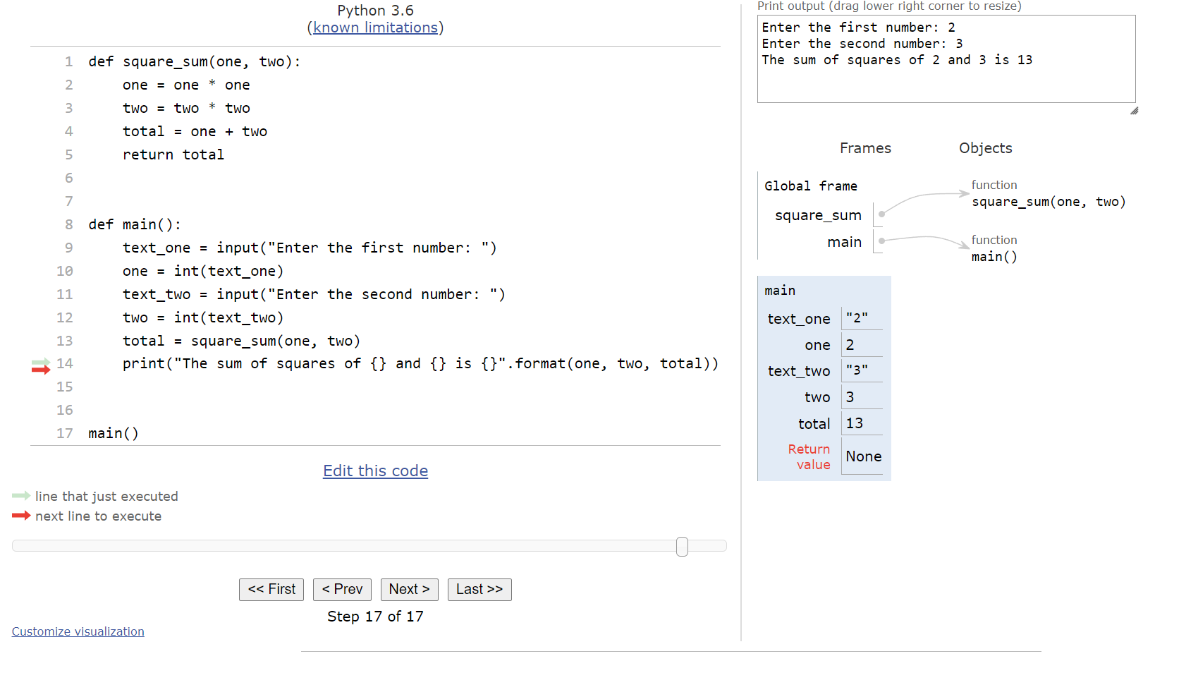
What’s also interesting to note here is the return value of the main() function. Since we didn’t include a return statement at the end of the function, the return value is set to a special value called None in Python. We’ll learn about what that value actually represents in a future course.
The entire process is shown in the animation below:
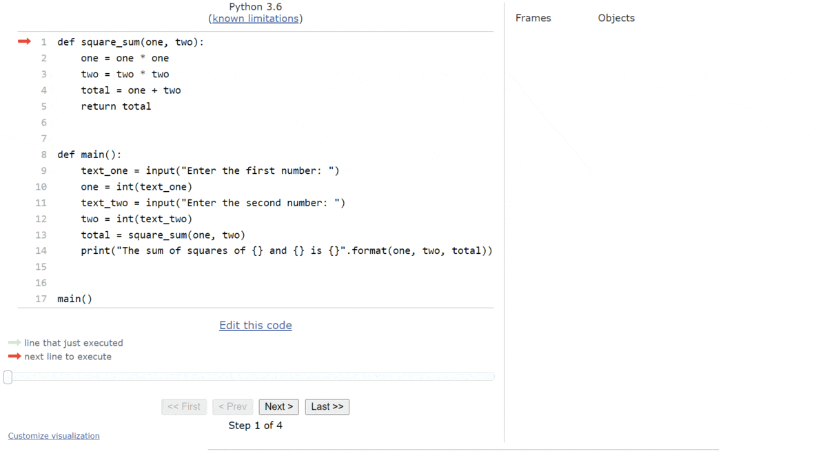
This review of how a function returns data should be very helpful as we continue to build more complex programs. Remember - we can always paste any Python code into a tool like Python Tutor to run through it step-by-step and see what it really does.
Finally, let’s look at how we can rewrite some of our previous Python programs by combining expressions into more complex statements. Just like we saw in pseudocode, Python also allows us to perform multiple actions on a single line of code, provided they can all be combined in some way to create a single statement.
Let’s consider the example on the previous page, shown here:
def square_sum(one, two):
    one = one * one
    two = two * two
    total = one + two
    return total


def main():
    text_one = input("Enter the first number: ")
    one = int(text_one)
    text_two = input("Enter the second number: ")
    two = int(text_two)
    total = square_sum(one, two)
    print("The sum of squares of {} and {} is {}".format(one, two, total))


main()
There are many ways we can write this program to perform the same work. For example, the square_sum() function can actually be reduced to a single line of code as seen below:
def square_sum(one, two):
    return (one * one) + (two * two)
We can perform multiple mathematical operations in a single expression, and as long as we either use parentheses or pay attention to the order of operations, we’ll get the expected answer. We don’t have to store the intermediate values in variables, since Python will do that for us when it evaluates the expression.
Likewise, in the main() function, we can put the input() expression inside of the int() function, allowing us to read input as a string and convert it to an integer in a single line:
def main():
    one = int(input("Enter the first number: "))
    two = int(input("Enter the second number: "))
    total = square_sum(one, two)
    print("The sum of squares of {} and {} is {}".format(one, two, total))
Finally, we can also move the function call to square_sum() directly into the format() method in the print() statement. When that line is executed, Python will know it has to call the square_sum() method first and get the returned value before it can print the output.
def main():
    one = int(input("Enter the first number: "))
    two = int(input("Enter the second number: "))
    print("The sum of squares of {} and {} is {}".format(one, two, square_sum(one, two)))
Of course, if we really wanted to, we could remove the square_sum() function entirely, and just compute the value directly in main(). However, for this example, we will leave it as a separate function. So, our new program contains this code:
def square_sum(one, two):
    return (one * one) + (two * two)


def main():
    one = int(input("Enter the first number: "))
    two = int(input("Enter the second number: "))
    total = square_sum(one, two)
    print("The sum of squares of {} and {} is {}".format(one, two, total))


main()
Functionally, this code will create the exact same output as the previous code, but it will do so using fewer variables and statements. Each statement is simply more complex, consisting of multiple expressions.
As we discussed in pseudocode, each of these approaches to writing code is valid. They simply follow different coding styles, each one with particular benefits and disadvantages to consider. Sometimes it is better to have more variables and shorter expressions, especially if the overall operation involves many steps and is difficult to follow. Other times it is better to combine a few lines of code together as a single statement to make it very clear what the overall operation is trying to accomplish.
Once again, the best advice is to simply write code in a way that it is readable to you and to anyone else who has to read it. As long as it is clear and performs correctly, it is a good style to follow. As we further develop our skills and gain experience, our style will continue to change over time.
In this lab, we covered several major important topics. Let’s quickly review them.
INPUT() will read input from the user and return what was typed as a string value.INPUT() is terminated by the user pressing ENTER, so next output starts on a new line.+ Concatenation (join strings together). May only be applied to two strings.RETURN(expression) will return the value of expression to where the procedure was called from.input(expression) will display the expression to the user as a prompt, then return what was typed by the user as a string value.input(expression) is terminated by the user pressing ENTER, so next output starts on a new line.+ Concatenation (join strings together). May only be applied to two strings.string.format(value1, value2) performs string formatting. The string portion is any valid template string, which contains curly braces {} as placeholders. Each placeholder will be replaced by the matching argument value1, value2, etc. from the format() method.return expression will return the value of expression to where the function was called from.Expressions can be combined in many ways within a statement. Expressions can be used as arguments to procedures, and more!
In pseudocode, we can create variables that store values using the Boolean data type. These variables can only store one of two values: true or false. So, a Boolean value is really the simplest data value we can imagine - it is a single binary bit representing a value of true or false. In some systems, we may also refer to these values as 0 or 1, but in pseudocode we’ll just use true and false.
To create a variable that stores a Boolean value in pseudocode, we can use the following assignment statements:
x <- true
y <- false
In pseudocode, both true and false are keywords in the language. They represent the special boolean values true and false, and cannot be used as the name of a variable or procedure. Since they are values and not strings, we do not have to put them in quotation marks.
We can use the special BOOLEAN() procedure to convert any value to a Boolean value. Here are the basic rules for that conversion:
"true" will evaluate to true and "false" will evaluate to false. Capitalization doesn’t matter. All other values are undefined.0 will evaluate to false, and any other value will be true.The reverse works as well - Boolean values can be provided as input to the STRING() or NUMBER() procedures, and the outputs produced there will match these rules. Specifically, the true value will convert to the number $1$, but any non-zero number would be valid.
There are also many special operators that can be used to perform operations on Boolean values. These operators are used to along with one or more Boolean values in some way to produce a resulting value. Let’s review the three important Boolean operators in pseudocode.
The first Boolean operator we’ll review is the AND operator. This operator is used to determine if both Boolean values are true, and if so the resulting value will also be true. Otherwise, it will be false. This corresponds to the following truth table:
| Variable 1 | Variable 2 | Result |
|---|---|---|
| F | F | F |
| F | T | F |
| T | F | F |
| T | T | T |
Here’s an example of using the AND operator in pseudocode:
x <- true
y <- true
z <- x AND y
DISPLAY(z)
When this code is executed, the following output should be displayed:
trueThe next Boolean operator to review in pseudocode is the OR operator. This operator will result in a true value if at least one of the input values is true. If both inputs are false, then the result is false. This corresponds to the following truth table:
| Variable 1 | Variable 2 | Result |
|---|---|---|
| F | F | F |
| F | T | T |
| T | F | T |
| T | T | T |
Here’s an example of using the OR operator in pseudocode:
a <- true
b <- false
c <- a OR b
DISPLAY(c)
When this code is executed, the following output should be displayed:
trueFinally, the other Boolean operator we’ll learn about is the NOT operator. This operator is only applied to a single Boolean value, and it is used to negate the value. This means that an input value of true will result in false, and vice-versa. This corresponds to the following truth table:
| Variable 1 | Result |
|---|---|
| F | T |
| T | F |
Here’s an example of using the NOT operator in pseudocode:
x <- true
y <- NOT x
DISPLAY(y)
Once again, when this code is executed, we’ll see the following output:
falseThese three operators allow us to perform the basic Boolean logic operations needed to build more complex programs.
Another powerful feature of pseudocode are the comparator operators, which can be used to create Boolean values by comparing string and number values in an expression. These comparators are a powerful way to build programs that can perform different actions based on data received from the user, as we’ll see later in this lab. Let’s review the commonly used comparators in pseudocode.
The equal comparator = is used to determine if two values are equivalent. This operator can be used between any two values, and it will either result in a value of true if both values are equivalent, or false if they are not. Here are some rules to keep in mind:
For example, we can use the equal comparator to check if two numeric values are equivalent, as shown in this example:
x <- 5
y <- 3 + 2
DISPLAY(x = y)
When executed, this code will display the following output:
trueWe can do the same for two strings:
a <- "Hello " + "World"
b <- "hello " + "world"
DISPLAY(a = b)
This time, the output will be:
falseThis is because the two string values are not identical - one has capital letters, and the other one does not.
In most other programming languages, the equality comparator is represented by two equals signs == instead of a single one =. This is because the single equals sign is used in assignment statements in most languages, so we use a double equal as the equality comparator to avoid any confusion between the two.
In pseudocode, we use the arrow symbol <- for assignment statements, so we can use the single equals sign for equality. However, it is important to remember that this only works in pseudocode, and will cause issues if used in other languages such as Python.
The next comparator is the not equal comparator, which is typically written as != in pseudocode. Sometimes, we may also see it formatted as the special character ≠, but we won’t use that character in our pseudocode.
The not equal comparator is exactly what it sounds like - it will return true if the two values being compared are not equivalent, or false if the two values are equivalent. So, the statement a != b is the same as saying NOT (a = b).
Here’s an example of using this comparator in pseudocode:
x <- 5
y <- 5 + 0.000001
DISPLAY(x != y)
When executed on our “mental model” of a computer, we should get the following output:
trueThis is because the values $5$ and $5.000001$ are not exactly the same value, even though they are very similar.
The last four comparators are all similar, so we’ll cover them all as a group. These comparators are specifically used to compare the relationship between two values, determining an ordering between the two. We should already be familiar with these operators from mathematics:
< less than<= less than or equal to (sometimes written as ≤ in text)> greater than>= greater than or equal to (sometimes written as ≥ in text)When these comparators are applied to numeric values, they’ll compare the two values just like we’d expect from math. For example, we can see these comparators in action in this pseudocode:
a <- 5
b <- 6
DISPLAY(a < b)
DISPLAY("\n")
DISPLAY(a > b)
When we run this code, we’ll see the following output:
true
false
These comparators are a bit more confusing when applied to string values. In that case, they will look at the lexicographic order of the two strings, which is similar to alphabetical order but also includes capitalization, punctuation, and other special symbols. We won’t cover that in too much detail here, but in most computer programs the letters are sorted according to their order in the ASCII encoding standard.
For example, we can compare two strings as shown in this example:
x <- "test"
y <- "tent"
DISPLAY(x < y)
When we run this program in our “mental model” of a computer, we’ll see this output:
falseThis is because the string "test" does not come before "tent" when placed in alphabetical order, since s comes after n. So, we would say that the string stored in x is not less than the string stored in y, and therefore the result should be false.
It’s also important to note that there are many situations where Boolean operators and mathematical operators are used in the same expression. In those cases, the mathematical operators are all resolved first, and then the Boolean operators in this order, going from left to right:
NOT operatorANDORAs always, it is considered good practice to include parentheses in any complex expressions to make sure that the intent is clear, regardless of the order of operations.
Let’s look at a quick example in pseudocode:
x <- 4 < 5 AND 3 * 5 > 12 OR NOT 7 MOD 3 = 1This expression includes many mathematical operators, as well as Boolean operators and comparators. To evaluate this expression, we must first resolve all mathematical operations first, so we’ll evaluate 3 * 5 and 7 MOD 3 and place those results in the expression:
x <- 4 < 5 AND 15 > 12 OR NOT 1 = 1Next, we’ll resolve any comparator operators, moving from left to right. This will convert any remaining numbers into Boolean values. So, we’ll evaluate 4 < 5, 15 > 12, and 1 = 1 and replace those expressions with the resulting Boolean values:
x <- true AND true OR NOT trueOnce we’ve done that, the next operator to evaluate is the NOT operator. So, we’ll evaluate NOT true to the resulting value false and place it back in the expression:
x <- true AND true OR falseThen, we’ll handle the AND operator, so we’ll evaluate true AND true to the value true:
x <- true OR falseFinally, we’ll evaluate the rest of the statement true OR false to the value true, which will be stored in the variable x:
x <- trueAs we can see, the order of operations allows us to work through a complex expression like this example. However, in practice, it is always best to include parentheses where needed to make sure the expression is evaluated like we intend it to be.
In Python, Boolean values are stored in the bool data type. Just like in pseudocode, variables of the bool data type can only store one of two values, True or False.
To create a Boolean variable in Python, we can simply assign those values to a variable in an assignment statement:
a = True
b = False
print(a)
print(type(b))
When we execute that code, we’ll see the following output:
True
<class 'bool'>
In Python, we use the keywords True and False to represent Boolean values. Notice that they are capitalized, unlike the true and false values we saw in pseudocode. In Python, it is very important to make sure these values are capitalized, otherwise the program will not work properly. Also, since these are keywords and not strings, we don’t need to put them in quotation marks.
Python includes the special bool() function, which can be used to convert any data type into a Boolean value. The bool() function follows these rules to determine what to return:
False, the value 0, the value None, or anything with 0 length, including the empty string, it will return False.True.Let’s look at a couple of quick examples. First, let’s try to convert the strings "True" and "False" to their Boolean equivalents:
print(bool("True"))
print(bool("False"))
When this code is executed, we’ll see this output:
True
True
This seems a bit strange, since the string "False" ended up creating the Boolean value True. However, if we look at the rules above, since the string "False" has a length greater than 1, and it is not any of the special values listed above, it should always result in the Boolean value True.
In this example, we can check a couple of special values using the bool() function:
print(bool(0))
print(bool(1))
print(bool(""))
In this case, we’ll see the following output:
False
True
False
Here, we see that the value 0, as well as the empty string "", both result in a value of False. However, the value 1 is True, since it is a non-zero value.
In practice, we won’t use the bool() function directly very often. Instead, if we want to determine if a user inputs a True or False value, we can just use one of the Boolean comparators that we’ll see later in this lab.
Python also includes several operators that can be applied to one or two Boolean values. These operators make up the basis of Boolean logic, and allow us to construct complex expressions of Boolean values. Let’s quickly review the three basic Boolean operators present in Python.
In Python, we use the keyword and to perform the Boolean and operation. Just like in pseudocode, this operator will return True if both input values are also True, otherwise it will return False.
Here’s a quick example of the and operator in Python:
x = True
y = False
print(x and y)
When we run this Python code, we should see this output:
FalseSince the variable y is False, the resulting value is also False.
Likewise, the keyword or is used in Python for the Boolean or operation. This operator will return True if either of the input values is True, but it will return False if neither of them are True.
Let’s look at an example:
a = False
b = True
print(a or b)
When we execute this code, we’ll get this output:
TrueSince b is True, we know that at least one input is True and the result of a or b is also True.
Finally, Python uses the keyword not to represent the Boolean not operation, which simply inverts a Boolean value from True to False and vice-versa.
Here’s an example:
x = True
print(not x)
print(not not x)
When we run this code, we’ll see this printed to the terminal:
False
True
Since x is True, we know that not x is False. We can then perform the not operation again, on that result, as shown in not not x, which will result in the original value of x, which is True.
Python also uses various comparators to allow us to compare values of many different data types to produce a Boolean value. We can compare numbers, strings, and many other data types in Python using these comparators.
Since we’ve already covered the comparators in pseudocode, let’s just briefly go over all of them and discuss any ways they differ in Python compared to pseudocode.
The basic comparators in Python are:
== equal!= not equal< less than<= less than or equal to> greater than>= greater than or equal toNotice that the equal comparator in Python now uses two equals signs == instead of a single one. This is because the single equals sign = is used in the assignment statement, and we don’t want to confuse a Boolean comparator for an assignment. So, in Python, as in most other programming languages, we use two equals signs == when comparing values, and one equals sign = when we are storing a value in a variable.
Just like in pseudocode, we usually only want to compare values of the same data type using comparators. It really only makes sense to compare strings to strings, and booleans to booleans. However, for the numeric data types int and float, we can easily compare values of either data type together in Python.
Consider the following example:
x = 5
y = 5.0
print(x == y)
When we execute this code, we’ll get this output:
TrueEven though x is the int data type and y is the float data type, they both store the same numerical value, and our comparators will work just like we expect. So, we can easily compare both integers and floating-point values in our code.
Behind the scenes, when we compare an int and a float value in Python, Python will convert the values to a common data type, usually the float data type, using the appropriate conversion function. This is known as coercion in programming - the program is essentially forcing a value of one data type into another data type because of an operation. However, it won’t change the data type of the variable involved, just the value it is evaluating.
Strings in Python can also be compared using the various comparator operators. When two strings are compared using any type of “less than” or “greater than” comparator, they will be compared according to their lexicographic order . In general, this means that each letter will be ordered based on its value in the ASCII encoding standard.
Let’s look at a quick example:
a = "First"
b = "fir"
print(a < b)
When we run this code, we’ll see this output:
TrueThis may seem surprising, since we’d expect the word "fir" to come before the word "First" in a dictionary, since it has fewer letters. However, in Python, the letters "f" and "F" are not treated identically. According to the ASCII
encoding standard, capital letters have a lower value than lower-case letters, so all words starting with a capital "F" will come before any words starting with a lower-case "f".
This can be a bit confusing, so it is always important to remember that we can always write a quick sample program in Python to test how a particular operator will work for a given set of values. If nothing else, we can always count on our computer to produce the same result for the same operation, no matter if it is part of a larger program or a small test program.
Finally, Python’s order of operations follow the same rules that we saw in pseudocode. So, when we see an expression that combines mathematical operators with Boolean operators and comparators, we’ll follow this order:
not operatorand operatoror operatorAs always, it is considered good practice to include parentheses in any complex expressions to make sure that the intent is clear, regardless of the order of operations.
In this lab, we covered several major important topics. Let’s quickly review them.
truefalseBOOLEAN() procedure to convert values
false, and any other number is trueANDORNOT= equal!= not equal< less than<= less than or equal to> greater than>= greater than or equal toTrueFalsebool() procedure to convert values
False, the value 0, the value None, or anything with 0 length, including the empty string, it will return False.True.andornot== equal!= not equal< less than<= less than or equal to> greater than>= greater than or equal toStrings are compared using lexicographic order
notandorNow that we understand how to use Boolean values in our pseudocode programs, it’s time to put those values to use. One way to think of the result of a Boolean expression is that it helps us make a decision in our programs. For example, if we want to do something special in our program when the user inputs the value $42$ into the variable x, then we can write the Boolean expression x = 42 to help us decide if the user input the correct value.
Once we have that decision made, we need some way to tell our program to run a different piece of code based on the outcome of that decision. In pseudocode, as well as most other programming languages, we can use a special construct called an if statement to do this. If statements are one example of a conditional statement in programming.
In an if statement, we start with a Boolean expression. Then, if that Boolean expression evaluates to the value true, we run the code inside of the if statement. Otherwise, we just skip that code and continue executing the rest of the program.
The general structure of an if statement in pseudocode is shown here:
IF(<boolean expression>)
{
    <block of statements>
}
In this structure, the <boolean expression> is any expression that results in a Boolean value. Typically, we use Boolean comparators and operators to construct the statement, along with any variables that are needed. Likewise, the <block of statements> is just like a block of statements inside of a procedure - it consists of one or more statements or lines of code, which can be executed.
To see how an if statement works, let’s go through a couple of code traces in an example program.
For this example, consider the following program in pseudocode:
PROCEDURE main()
{
    DISPLAY("Enter a number: ")
    x <- NUMBER(INPUT())
    IF(x = 42)
    {
        DISPLAY("You found the secret!\n")
    }
    DISPLAY("Thanks for playing!\n")
}

main()
Let’s run trace through this program a couple of times to see how an if statement works in pseudocode. As always, we’ll start our code trace as shown below:
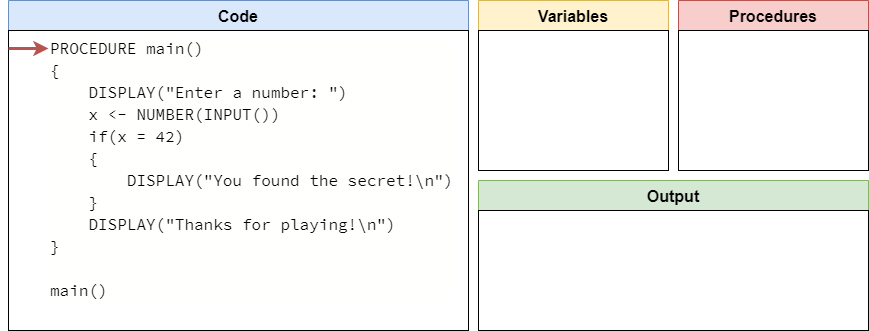
Next, we’ll process through the code, finding our main() procedure. At the end, we’ll reach the call for the main() procedure:
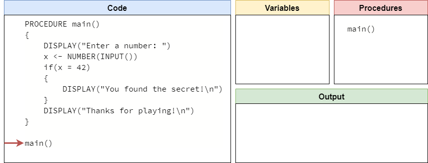
So, we’ll enter the main() procedure here.
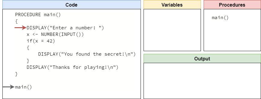
The first line of code will display a prompt to the user:
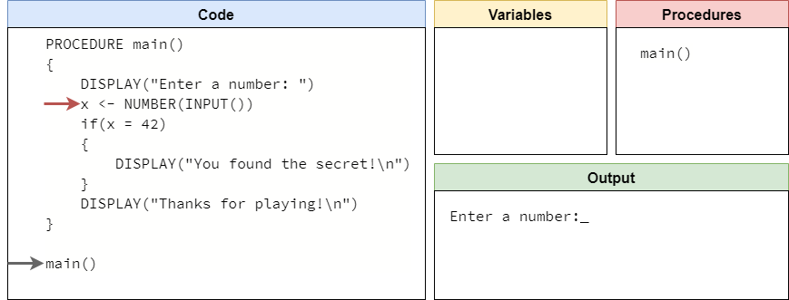
Then, we’ll read the input from the user and convert it to a number. In this example, let’s assume the user inputs the value "16" at the prompt. So, we’ll store the number value $16$ in the variable x.
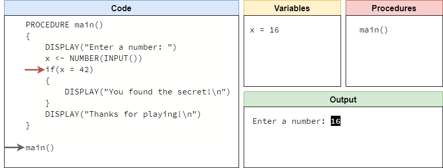
Now we have reached the beginning of the if statement in our code. When we evaluate an if statement, the first thing we need to do is evaluate the Boolean expression inside the parentheses. In this example, we are evaluating the expression x = 42. Since x is $16$, this evaluates to false:
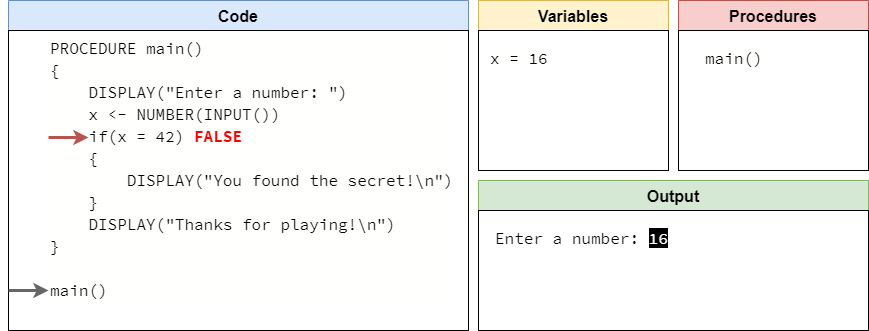
When the Boolean expression is false, we don’t execute the code inside of the if statement’s curly braces {}. So, we’ll just skip to the bottom of the statement, and execute the next line:
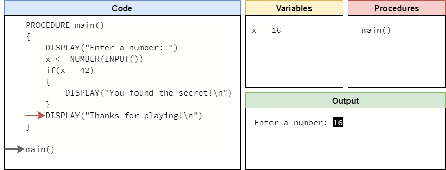
This line simply displays a message to the user, and then the program ends:
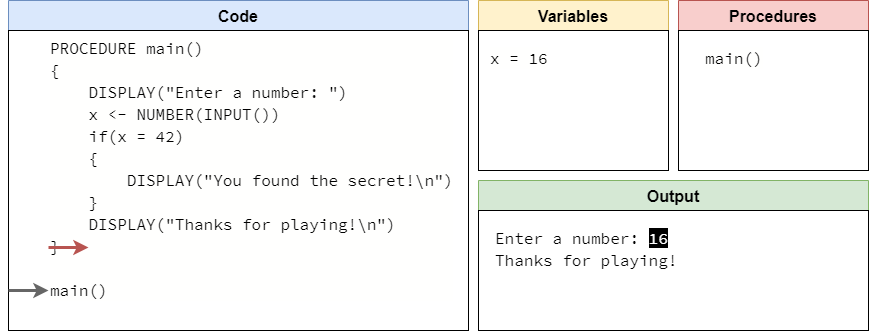
This entire process is shown in the animation below:

Now let’s go back a few steps in the program to the point where it is expecting user input:
This time, let’s assume the user inputs the value "42" at the prompt. So, that means that the variable x will now store the value $42$ as shown here:

Now, when we reach the beginning of the if statement, we’ll evaluate the expression x = 42 again, but this time the result will be true since x is indeed storing the value $42$:

When the Boolean expression is true in an if statement, we should execute the code inside its curly braces {}. So, we’ll move the arrow down to that line:
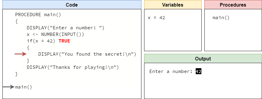
This line will print out special output for the user, as shown here:
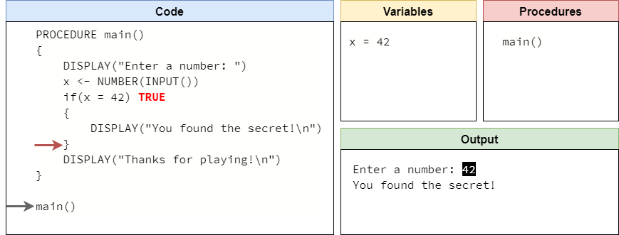
Once we’ve reached the end of the block of statements inside of the if statement, we’ll just continue through the program starting with the next line of code after the if statement:
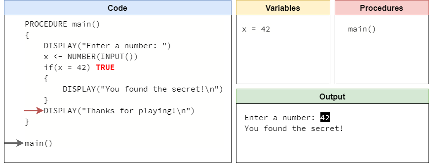
This line will print a message as well, and then the program will end:
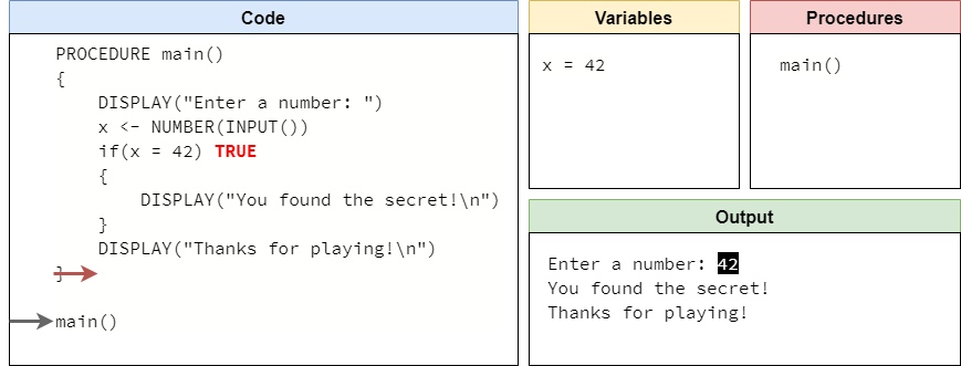
This entire process is shown in the animation below:
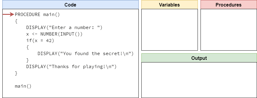
As we can see, an if statement is a powerful construct in our program. We can use any variables to create a Boolean expression using comparators and operators, and then we can use that result to make a decision about whether to run a special piece of code or not.
Another way to visualize an if statement is using a flowchart. Consider the following pseudocode:
x <- NUMBER(INPUT())
IF(x > 0)
{
    DISPLAY(x)
}
DISPLAY("Goodbye")
This pseudocode can also be represented as the flowchart shown below:
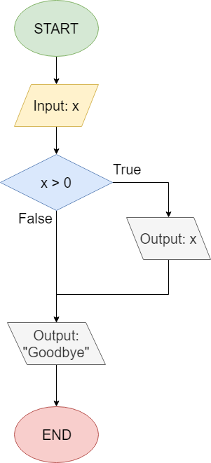
When we read flowcharts like this, we typically go from top to bottom, starting with the circle labeled “START”. The first step is to read input from the user, and store that value in the variable x.
Then, we reach a decision node, which uses a diamond shape. This node asks if the value in the variable x is greater than 0. Notice that there are two lines coming from the decision node: one labeled “True” and another labeled “False”. They correspond to the possible values that can result from evaluating the Boolean expression x > 0. So, if the result of that expression is true, then we’ll follow the path that exits the diamond from the side labeled “True”, and we’ll output the value x to the terminal. Once that is done, we can follow that path around to the next box that will output the string "Goodbye".
If that result is false, then we’ll follow the downward path labeled “False” and skip the path to the side. Instead, we’ll just reach the line that prints "Goodbye" and then end the program.
As we learn how to use if statements in our code, we might find it easier to use flowcharts or other tools to help understand exactly what our program will do. The path that a program takes through a flowchart like this is called the control flow of the program. We’ll discuss that topic a bit more toward the end of this lab.
Another important type of conditional statement is the if-else statement. In an if-else statement, we can run either one piece of code if the Boolean expression evaluates to true, or another piece of code if it evaluates to false. It will always choose one option or the other, based on the value in the Boolean expression.
The general structure of an if-else statement in pseudocode is shown here:
IF(<boolean expression>)
{
    <block of statements 1>
}
ELSE
{
    <block of statements 2>
}
In this structure, the <boolean expression> is any expression that results in a Boolean value. Typically, we use Boolean comparators and operators to construct the statement, along with any variables that are needed. In an if-else statement, unlike an if statement, we see two blocks of statements. The first block of statements, labeled <block of statements 1>, will only be executed if the <boolean expression> evaluates to true. Similarly, the second block of statements, labeled <block of statements 2>, will only be executed if the <boolean expression> evaluates to false. So, our program is effectively choosing between one block of statements or the other, based on the value in the Boolean expression.
To see how an if-else statement works, let’s go through a couple of code traces in an example program.
For this example, consider the following program in pseudocode:
PROCEDURE main()
{
    DISPLAY("Enter a number: ")
    x <- NUMBER(INPUT())
    IF(x MOD 2 = 0)
    {
        DISPLAY("Your number is even!\n")
    }
    ELSE
    {
        DISPLAY("Your number is odd!\n")
    }
    DISPLAY("Thanks for playing!\n")
}

main()
This program will accept input from the user, and then determine if the user has input an even or odd number using the modulo operator. Let’s run trace through this program a couple of times to see how an if-else statement works in pseudocode. As always, we’ll start our code trace as shown below:
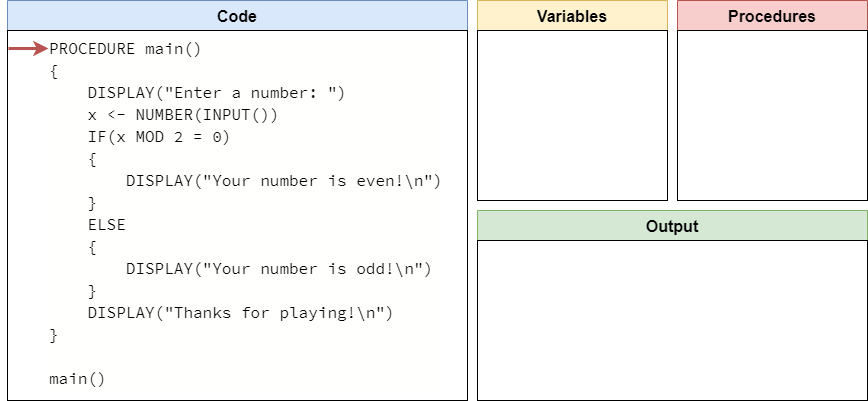
Just like always, our “mental model” of a computer will first skim through the code to find all of the procedures, and then it will reach the call to the main() procedure at the bottom of the code as shown here:
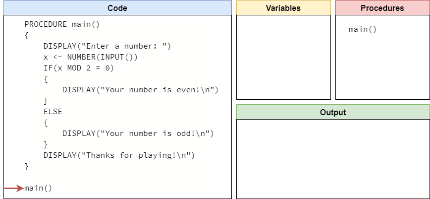
So, we’ll jump inside the main() procedure, and start running the code that is present there:
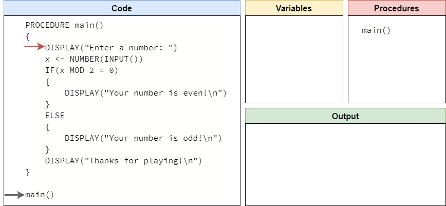
This first line will simply print a prompt for input to the user, so we’ll add that to the output and move to the next line as shown below:
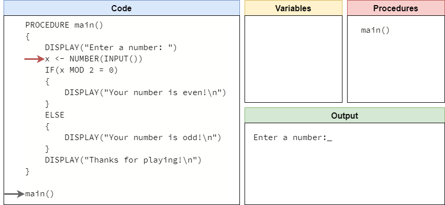
On this line, we’ll read input from the user, convert it to a number, and store it in the variable named x. In this example, let’s assume the user inputs the string "16". In that case, we’ll store the number value $16$ in the variable x as shown in this code trace:

At this point, we’ve reached the first part of our if-else statement. So, the first step is to evaluate the Boolean expression in parentheses and determine if it is either true or false. In this case, our expression is x MOD 2 = 0, so we need to start by evaluating x MOD 2. Recall that the modulo operation will find the remainder of dividing the first number by the second number. Since $2$ goes evenly into $16$ exactly $8$ times, with no remainder, we’ll get the value $0$. So, this expression is really the Boolean expression 0 = 0, which is true:
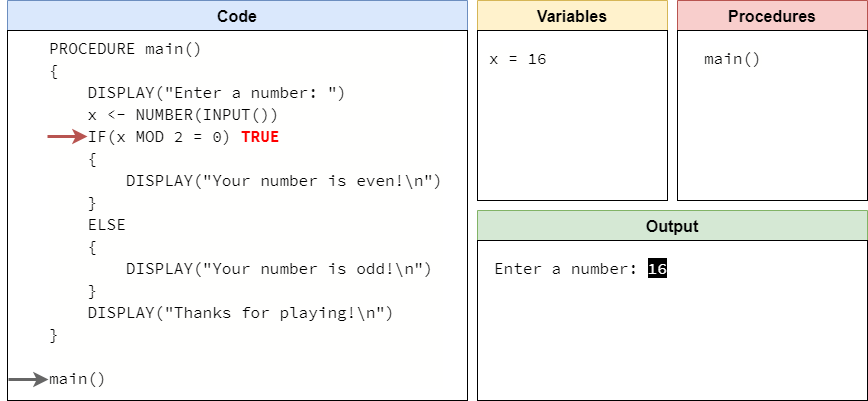
Since the Boolean expression is true, then our program will move to the first block of statements inside the if-else statement, and start executing that code:
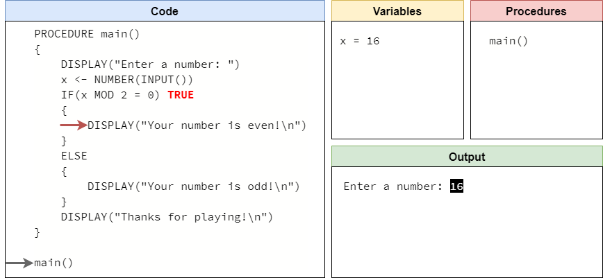
This line will print a message to the user that the number provided as input was even, so we’ll display that in our output:
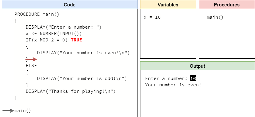
At this point, we’ve reached the end of that block of statements, so we need to figure out where to go next. Since this is an if-else statement, and the Boolean expression was true, that means we can just skip the second block of statements and go straight down to the first line of code after the if-else statement, as shown here:

This line will print our goodbye message to the user, so we’ll show that in our output and move to the end of the main() procedure:
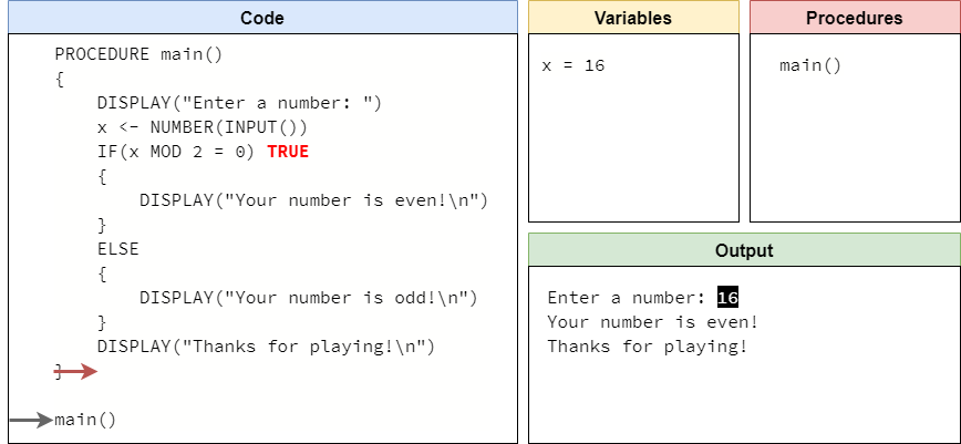
This is the end of that execution of our program. The entire process is shown in the animation below:
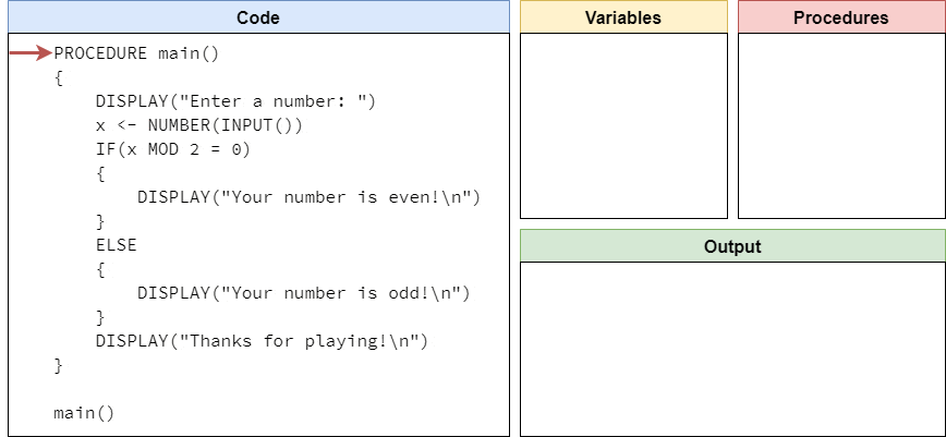
Once again, let’s go back a few steps in the program to the point where it is expecting user input:
This time, let’s say the user chooses to input the string "13" instead. So, we’ll store the number value $13$ in the variable x as shown in this code trace:
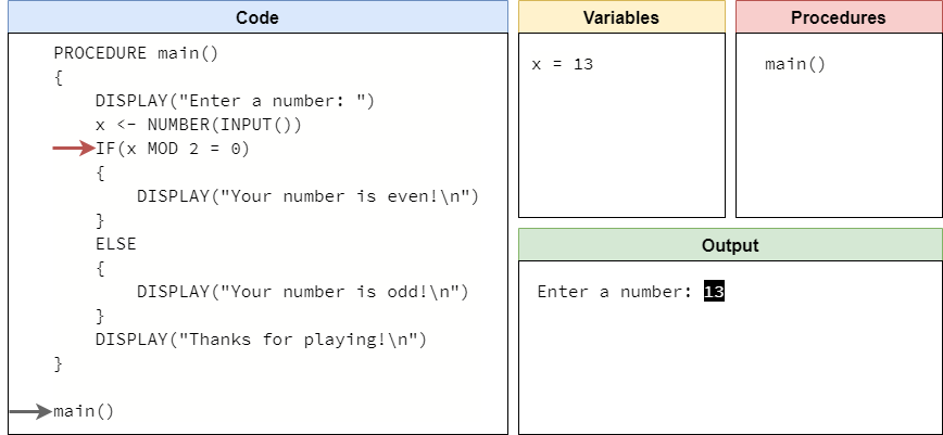
Now we’re back at the start of our if-else statement, but this time when we evaluate the Boolean expression x MOD 2 = 0, we’ll find out that the remainder of dividing $13$ by $2$ is $1$, since $2$ will only go into $13$ a total of $6$ times, for a value of $12$ with $1$ lefover as the remainder. So, since 1 = 0 is is not true, our Boolean expression will evaluate to false:
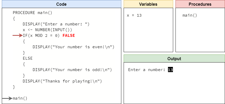
In this case, our if-else statement will jump down to the second block of statements as shown here:
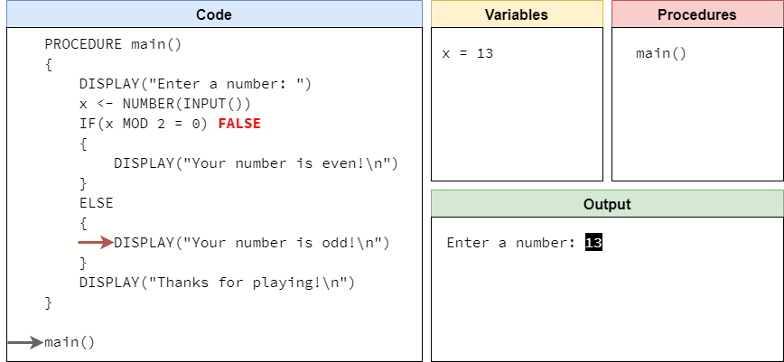
This statement will display output to the user showing that the provided value was odd, as we can see here:
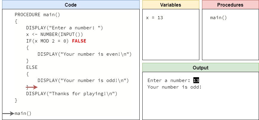
At this point, we’ve reached the end of that block of statements. So, just like when we reached the end of the first block of statements, we can now jump down to the first line of code after the if-else statement:

Once again, this will print our goodbye message to the user:
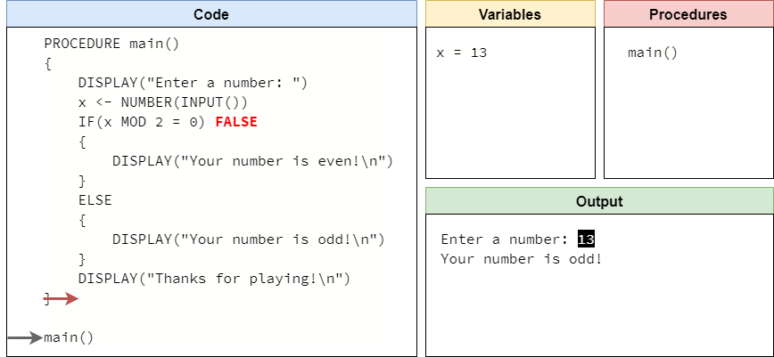
We’ll reach the end of our program here. A full run of this program is shown in the animation below:
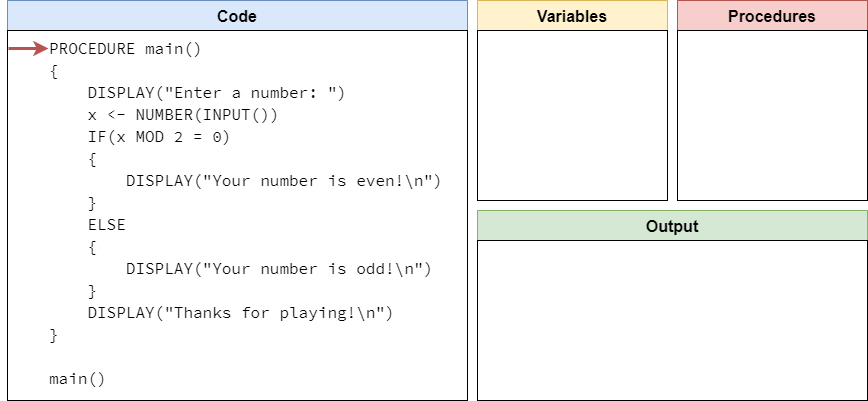
Another way to visualize an if-else statement is using a flowchart. Consider the following pseudocode:
x <- NUMBER(INPUT())
IF(x >= 0)
{
    DISPLAY(x)
}
ELSE
{
    DISPLAY(-1 * x)
}
DISPLAY("Goodbye")
This pseudocode can also be represented as the flowchart shown below:
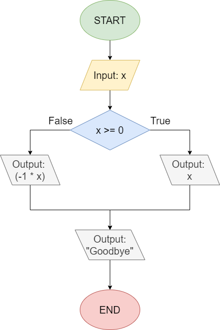
Once again, we start at the top of the flowchart at the circle labeled “START”. From there, we read an input from the user and store it in the variable x. At this point, we reach our if-else statement’s decision node, represented by the diamond. Here, we are using the Boolean expression x >= 0 to determine which branch to follow. So, if the user inputs a positive value, then we’ll follow the path to the right that is labeled “True”, which will simply print the value of x to the screen.
However, if the user inputs a negative value for x, then the Boolean expression will be false and we’ll follow the path to the left labeled “False”. In this branch, we’ll print the value of (-1 * x) to the screen, which simply removes the negative sign from the value in x.
Finally, after each path, we’ll merge back together to run the last piece of code, which prints the "Goodbye" message to the screen.
Notice that there is no way to print both x and -1 * x in the same execution of this program. If we follow the arrows through the flowchart, we see that we can only follow one branch or the other, and not both. This is an important concept to remember when working with if-else statements! The control flow of the program can only pass through one of the two blocks of statements, but not both.
One important concept to understand when writing if statements and if-else statements is the control flow of the program. Before we learned about conditional statements, our programs had a linear control flow - there was exactly one pathway through the program, no matter what. Each time we ran the program, the same code would be executed each time in the same order. However, with the introduction of conditional statements, this is no longer the case.
Because of this, testing our programs becomes much more complicated. We cannot simply test it once or twice, but instead we should plan on testing our programs multiple times to make sure they work exactly the way we want. So, let’s go through some of the various ways we can test our programs that include conditional statements.
First, let’s consider this example pseudocode program:
PROCEDURE main()
{
    DISPLAY("Enter a number: ")
    x <- NUMBER(INPUT())
    DISPLAY("Enter another number: ")
    y <- NUMBER(INPUT())
    IF (x + y > 10)
    {
        DISPLAY("Branch 1")
    }
    ELSE
    {
        DISPLAY("Branch 2")
    }
    IF (x - y > 10)
    {
        DISPLAY("Branch 3")
    }
    ELSE
    {
        DISPLAY("Branch 4")
    }
}

main()
We can represent the two if-else statements in this pseudocode in the following flowchart as well:
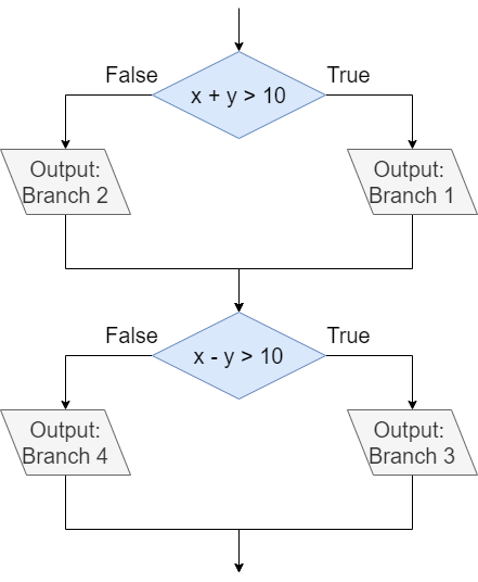
First, let’s consider how we can achieve branch coverage by executing all of the branches in this program. This means that we should test the program using different sets of inputs that will run different branches in the code. Our goal is to execute the code in each branch at least once. In this example, we see that there are four branches, helpfully labeled with the numbers one through four in the DISPLAY() statements included in each branch.
So, let’s start with a simple set of inputs, which will store $6$ in both x and y. Which branches will be executed in this case? Before reading ahead, see if you can work through the code above and determine which branches are executed?
In the first if-else statement, we’ll see the x + y is equal to $12$, which is greater than $10$, making that Boolean statement true. So, we’ll execute the code in branch 1 this time through. When we reach the second if-else statement, we’ll compute the value of x - y to be $0$, which is less than $10$. In this case, that makes the Boolean statement false, so we’ll execute branch 4. Therefore, by providing the inputs 6 and 6, we’ve executed the code in branches 1 and 4.
So, can we think of a second set of inputs that will execute the code in branches 2 and 3? That can be a bit tricky - we want to come up with a set of numbers that add to a value less than $10$, but with a difference that is greater than $10$. However, we can easily do this using negative numbers! So, let’s assume that the user inputs $6$ for x and $-6$ for y. When we reach the first if-else statement, we can compute the result of x + y, which is $0$. That is less than $10$, so the Boolean statement is false and we’ll execute the code in branch 2. So far, so good!
Next, we’ll reach the second if-else statement. Here, we’ll compute the result of x - y. This time, we know that $6 - -6$ is actually $12$, which is greater than $10$. So, since that Boolean expression is true, we’ll run the code in branch 3. That’s exactly what we wanted!
Therefore, if we want to test this program and try to execute all the branches, we only have to provide two pairs of inputs:
However, that’s only one way we can test our program. There are many other methods we can follow!
A more thorough way to test our programs is to achieve path coverage. In this method, our goal is to execute all possible paths through the program. This means that we want to execute every possible ordering of branches! So, since our program has 4 branches in two different if-else statements, the possible orderings of branches are listed below:
As we can see, there are twice as many paths as there are branches in this case! We’ve already covered ordering 2 and 3 from this list, so let’s see if we can find inputs that will cover the other two orderings.
First, we want to find a set of inputs that will execute branch 1 followed by branch 3. So, we’ll need two numbers that add to a value greater than 10, but their difference is also greater than 10. So, let’s try the value $12$ for x and $0$ for y. In that case, their sum is greater than $10$, so we’ll execute branch 1 in the first if-else statement. When we reach the second if-else statement, we can evaluate x - y and find that it is also $12$, which is greater than $10$ and we’ll execute branch 3. So, we’ve covered the first ordering!
The last ordering can be done in a similar way - we need a pair of inputs with a sum less than $10$ and also a difference less than $10$. A simple anwer would be to input $4$ for both x and y. In this case, their sum is $8$ and their difference is $0$, so we’ll end up executing branch 2 of the first if-else statement, and branch 4 of the second if-else statement. So, that covers the last ordering.
As we can see, path coverage will also include branch coverage, but it is a bit more difficult to achieve. If we want to cover all possible paths, we should test our program with these 4 sets of inputs now:
There’s still one more way we can test our program, so let’s try that out as well.
Finally, we should also use a set of inputs that test the “edges” of the Boolean expressions used in each if-else statement. An edge is a value that is usually the smallest or largest value before the Boolean expression’s output would change. So, an edge case is simply a set of input values that are specifically created to be edges for the Boolean expressions in our code.
For example, let’s look at the first Boolean logic statement, x + y > 10. If we are simply considering whole numbers, then the possible edge cases for this Boolean expression are when the sum of x + y is exactly $10$ and $11$. When it is $10$ or below, the result of the Boolean expression is false, but when the result is $11$ or higher, then the Boolean expression is true. So, $10$ and $11$ represent the edge between true values and false values. The same applies to the Boolean expression in the second if-else statement.
So, to truly test the edge cases in this example, we should come up with a set of values with the sum and difference of exactly $10$ and exactly $11$. For the first one, a very easy solution would be to set x to $10$ and y to $0$. In this case, both the sum and the difference is $10$, so we’re on the false side of the edge. Our program will correctly execute branches 2 and 4.
For the other edge, we can use a similar set of inputs where x is $11$ and y is still $0$. In this case, both the sum and difference is $11$, so each Boolean expression will evaluate to true and we’ll execute branches 1 and 3.
Why is this important? To understand that, we must think a bit about what was intended by this program. What if the program should execute branches 1 and 3 if the value is greater than or equal to $10$? In that case, both of our chosen edge cases should execute branches 1 and 3, but instead we saw that the edge case $10$ executed branches 2 and 4 instead. This is a simple logic error that happens all the time in programming - we simply forgot to use the greater than or equal to symbol >= instead of the simple greater than symbol > in our code. So, a minor typo like that can change the entire execution of our program, and we wouldn’t have noticed it in any of our previous tests. This is why it is important to test the edge cases along with other inputs.
In fact, it would probably be a good idea to add a third edge case, where the sum and difference equal $9$, just to be safe. That way, we can clearly see the difference between true and false values in this program.
So, the final set of values we may want to test this program with are listed below:
As we can see, even a simple program with just a few lines of code can require substantial testing to really be sure it works correctly! This doesn’t even include other types of testing, where we make sure it works properly with invalid input values, decimal numbers, and other situations. That type of testing is really outside of the scope of this lab, but we’ll learn more about some of those topics later in this course.
Boolean expressions in Python can be used in a variety of ways. One of the most important things we can do with a Boolean expression is affect the control flow of our program using a conditional statement.
Recall that a conditional statement is a type of statement that allows us to choose to run different pieces of code based on the value given in a Boolean expression. The simplest conditional statement is the if statement.
In an if statement, we include a Boolean expression and a block of statements. If the Boolean expression evaluates to True, then we execute the code in the block of statements. If it is False, then we skip the block and continue with the rest of the program.
The structure of an if statement in Python is shown below:
if <boolean expression>:
    <block of statements>
In this structure, we still have a <boolean expression> that is evaluated. However, instead of it being in parentheses like in pseudocode, in Python those parentheses are not required. After the Boolean expression is a colon :, just like at the end of a function definition.
Then, the <block of statements> is included below the if statement’s first line, and it must be indented one level. Again, this is very similar to the structure of a function definition in Python. In Python, the <block of statements> must include at least one line of code, otherwise Python won’t be able to understand it.
Let’s go through a couple of code tracing examples in Python Tutor to see how an if statement works in code.
Consider this program in Python:
def main():
    x = int(input("Enter a number: "))
    if x == 7:
        print("That's a lucky number!")
    print("Thanks for playing!")


main()
We can run that code in Python Tutor by clicking this Python Tutor link. At first, our window should look something like this:
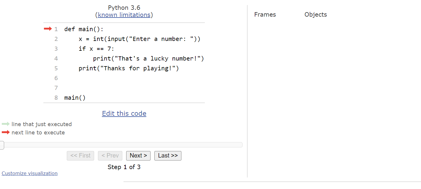
When we step through the program, the first thing it will do is record the main() function in the objects list, as shown here:
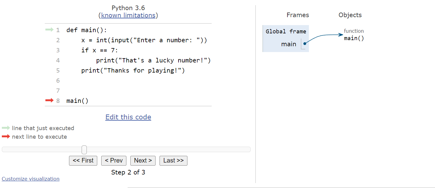
Then, we’ll reach the call to the main() function, so Python Tutor will jump to that function and create a frame for all the variables needed:
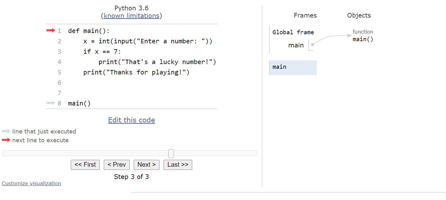
The next line of code will ask the user to input a number, so Python Tutor will show an input box at the bottom of the window:
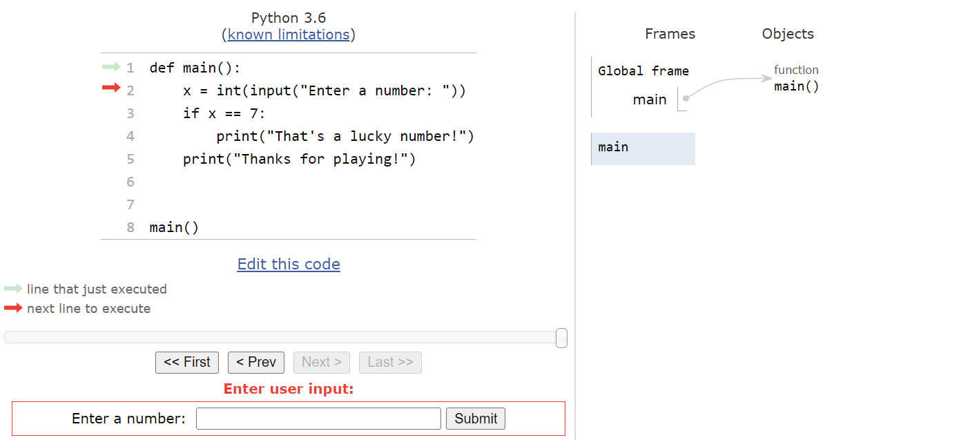
For this first time through the program, let’s assume the user inputs the string "42" as input. So, when we click Submit, we’ll see the integer value $42$ stored in the variable x in the main frame:
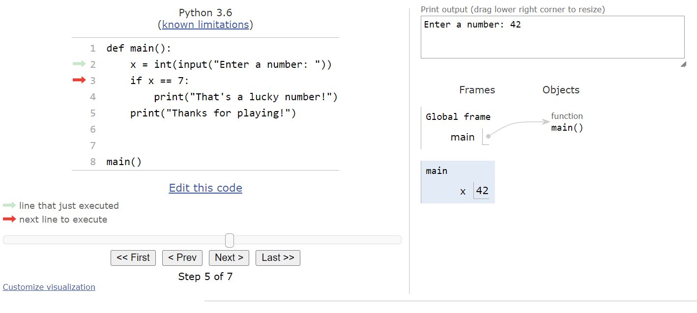
At this point, we’ve reached the if statement. The first step is to evaluate the Boolean expression x == 7. Since x is actually storing the value $42$, this statement will evaluate to False. So, when we click the Next button on the state below:
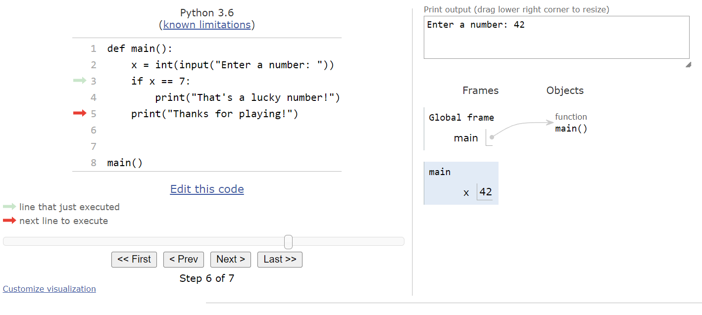
We’ll see that the program arrow jumps past the block of statements in the if statement. So, the next line will simply print the goodbye message:
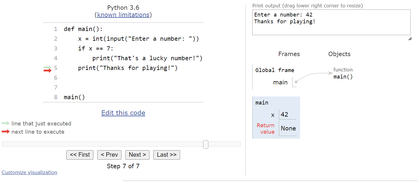
Finally, the main() function will return, and we’ll end the program:
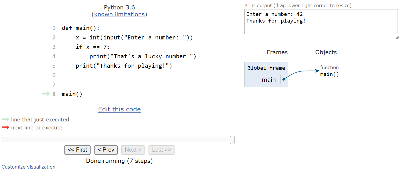
The entire process is shown in the animation below:

As we can see, when the Boolean expression evaluates to False, we’ll just skip the block of statements inside of the if statement. This is the same result that we observed when we were working in pseudocode.
Now let’s see what happens when the Boolean expression evaluates to True instead. To see that, we can go back to the point where our program is asking for input, as shown below:
This time, we’ll assume the user inputs the string "7" as input. So, when we click Submit, we’ll see the integer value $7$ stored in the variable x in the main frame:

This time, when we reach the if statement, we’ll see that the Boolean expression x == 7 will evaluate to True. So, when we click the Next button, we’ll be taken to the block of statements inside of the if statement:
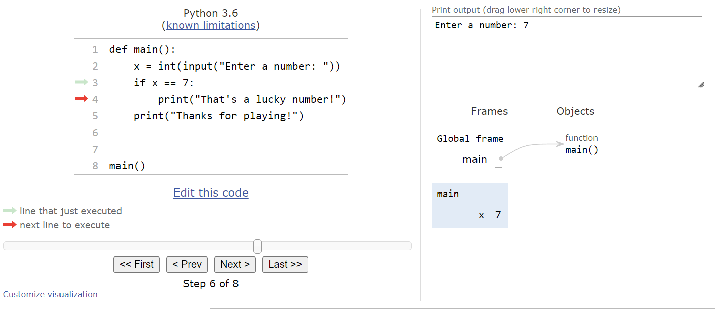
Here, we’ll print the special message for finding a lucky number:
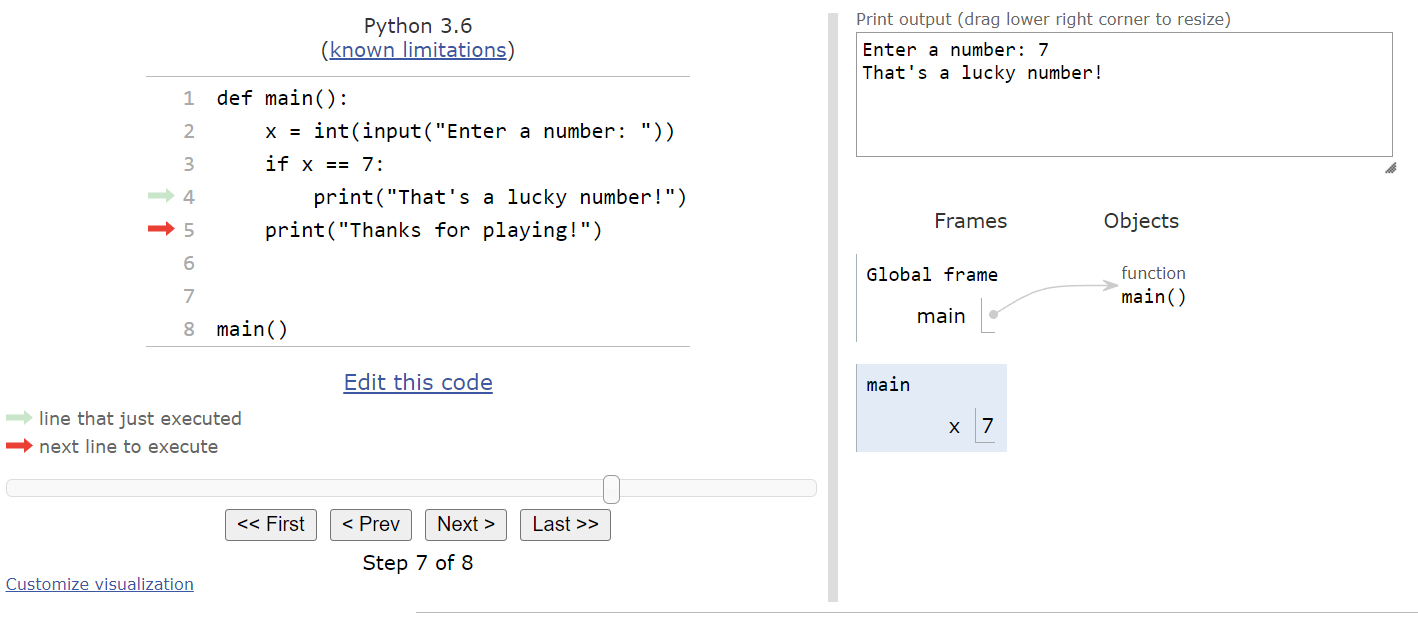
Then, we’ll print the program’s goodbye message:
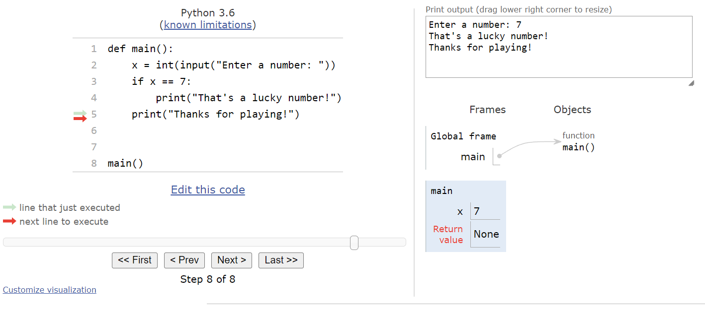
And finally we’ll reach the end of the main() function, so it will return and we’ll be at the end of the program:
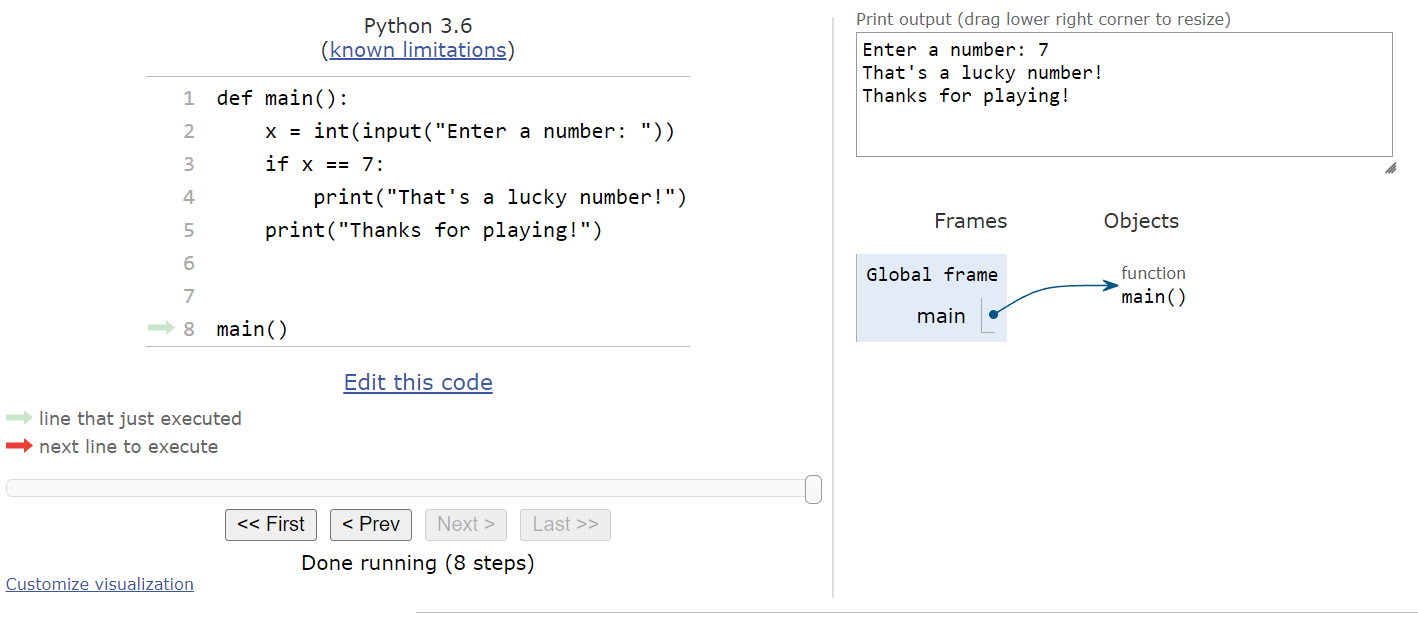
The entire process can be seen in this animation:
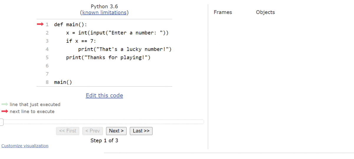
So, when the Boolean expression evaluates to True, we’ll run the code inside the if statement. If it is False, then we’ll just skip past the if statement and continue with the rest of our program.
Python also supports another kind of conditional statement, the if-else statement. Just like in pseudocode, an if-else statement contains a single Boolean expression, but two blocks of code. If the Boolean expression evaluates to True, then one block of statements is executed. If it is False, then the other block will be executed.
The general structure of an if-else statement in Python is shown below:
if <boolean expression>:
    <block of statements 1>
else:
    <block of statements 2>
Notice that the else keyword is followed by a colon, just like the first line of the if-else statement. As we’d expect, the first block of statements is executed if the <boolean expression> portion is True and the second block is executed if it is False.
Once again, let’s go through a couple of code traces using Python Tutor to explore how an if-else statement works in Python.
Here’s a simple Python program that contains an if-else statement:
def main():
    x = int(input("Enter a number: "))
    if x >= 0:
        print("Your number is positive!")
    else:
        print("Your number is negative")
    print("Thanks for playing!")


main()
This program accepts an input from the user, converts it to an integer, and then determines if the integer is a positive or negative number. Let’s go through this program a couple of times in Python tutor to see how it works. As always, you can click this Python Tutor link:
We’ll start with the usual default state:

Like always, Python will find the main() function and add it to the objects list. Then, it will call the main() function, and we’ll be presented with an input prompt as shown here:
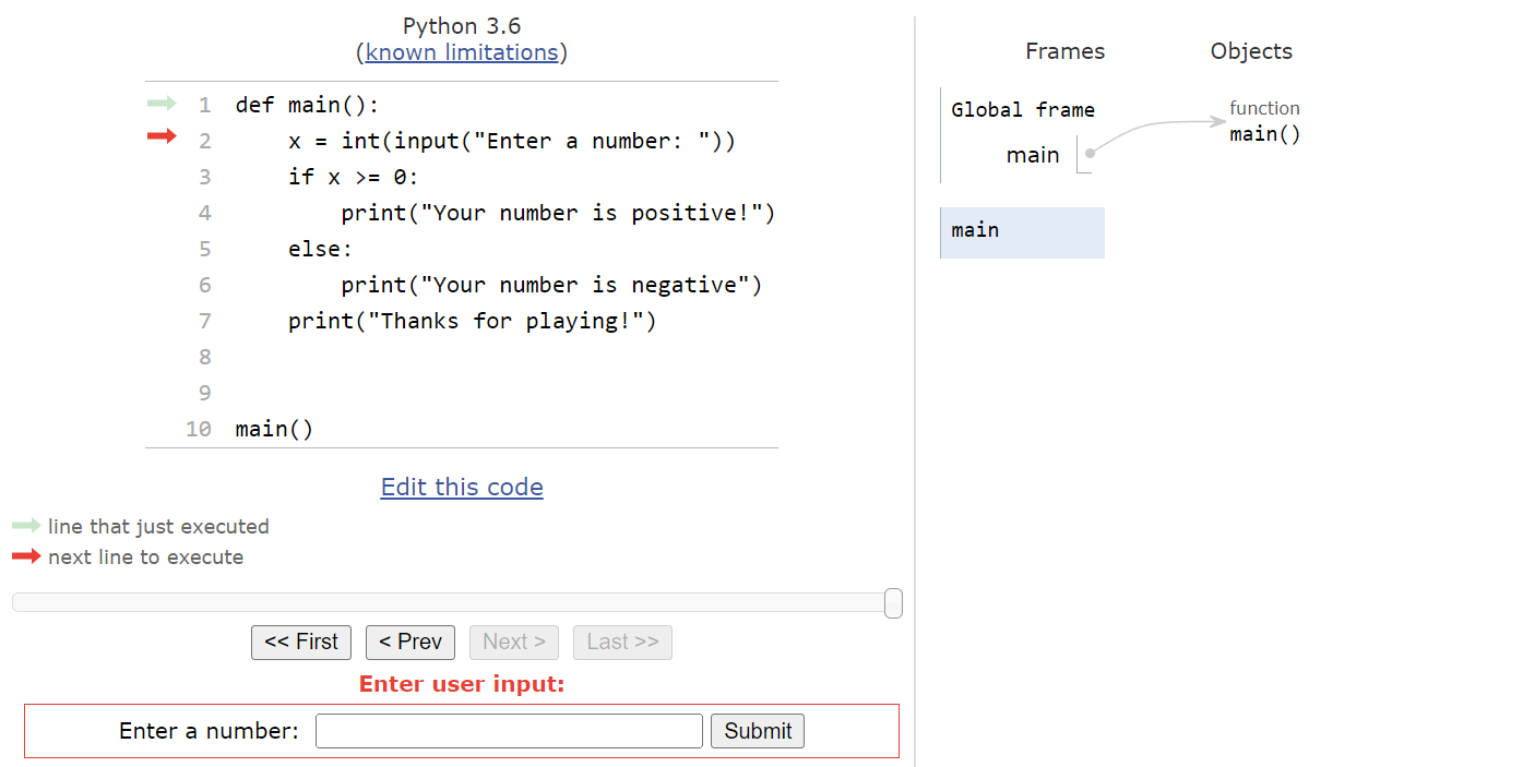
Let’s assume that the user inputs the string "5" here. That means that the integer value $5$ will be stored in the variable named x:
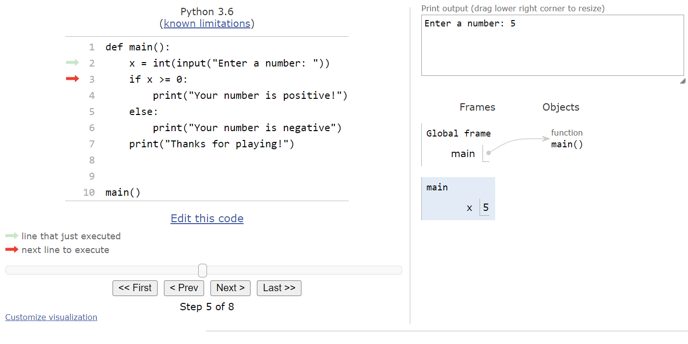
Now we’ve reached the if-else statement. So, we’ll need to evaluate the Boolean expression x >= 0. Since x is currently storing the value $5$, this expression will evaluate to True. Therefore, we’ll move into the first block of statements in the if-else statement:

From here, we’ll print the message that the user’s input was a positive number, as well as the goodbye message at the end of the program. It will entirely skip the second block of statements in the if-else statement, as we can see here:
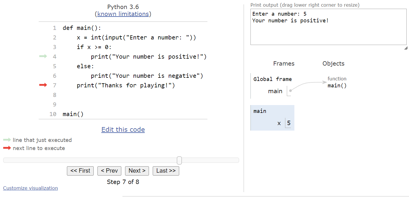
A full execution of this program is shown in the animation below:
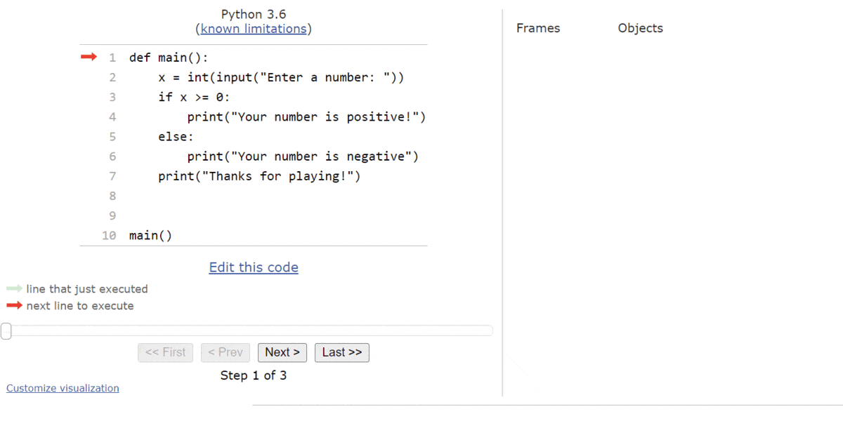
What if the user inputs a negative value, such as $-7$? In that case, we’ll be at this state in our program:

From here, we’ll evaluate the Boolean expression x >= 0 again. This time, however, we’ll see that it evaluates to False, so we’ll jump down to the second block of statements inside the if-else statement:

This will print a message to the user that the input was a negative number, and then it will print the goodbye message. We completely skipped the first block of statements:
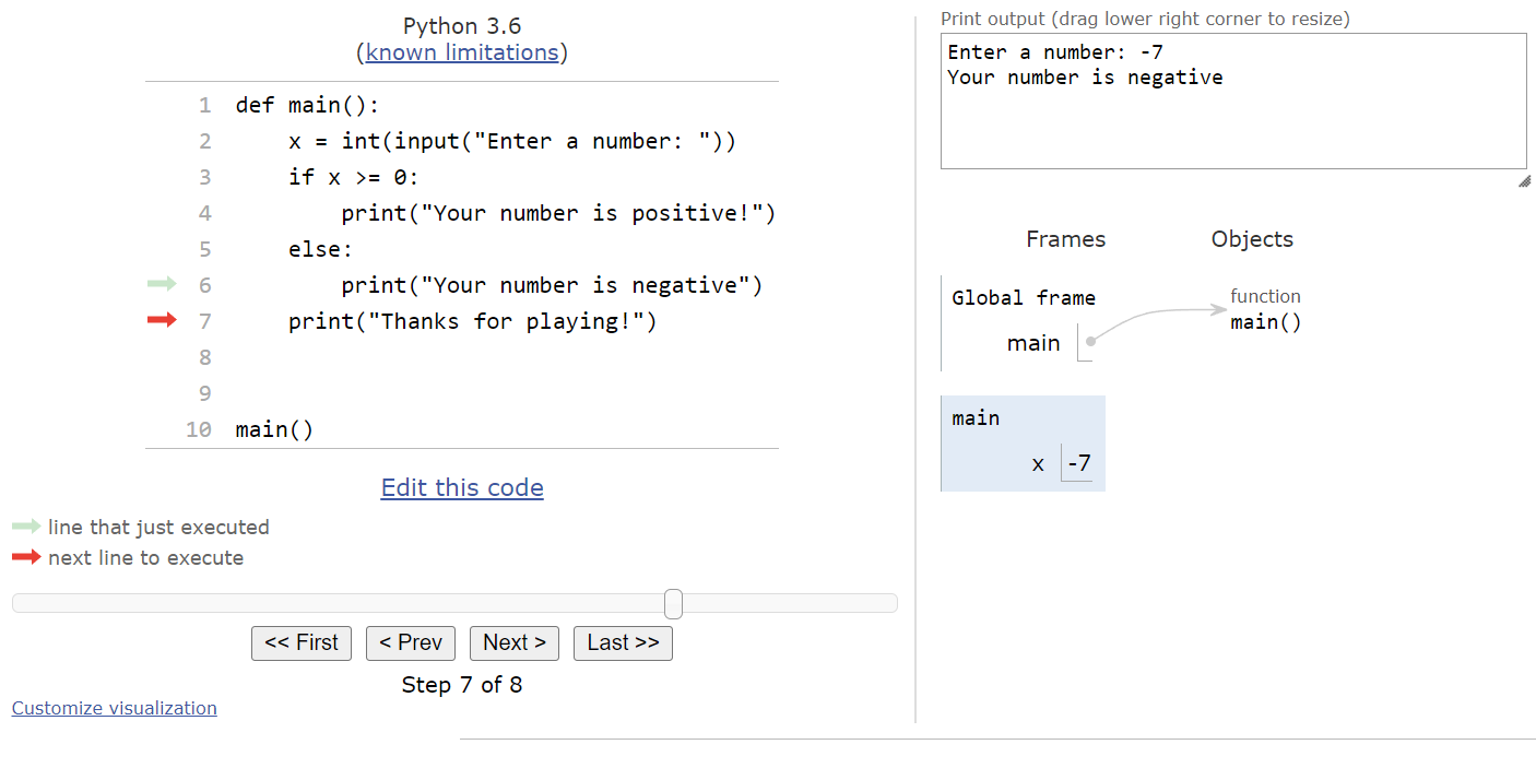
A complete run through this program is shown in this animation:
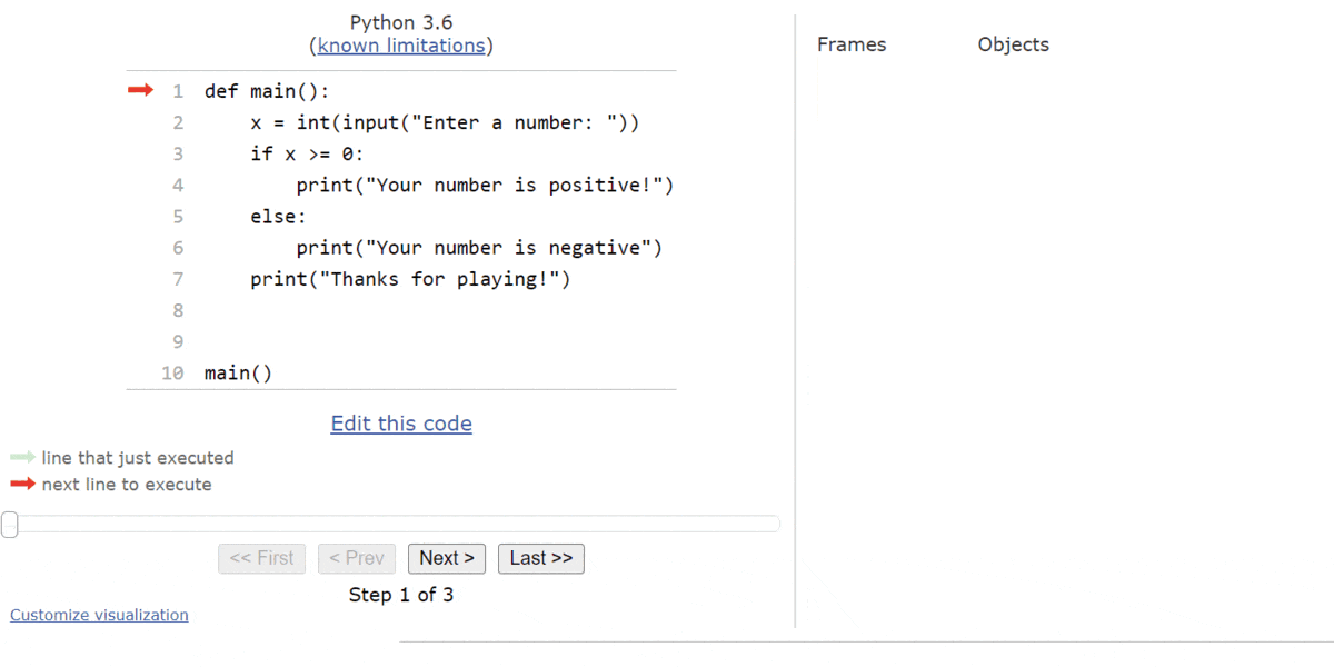
So, as we expect, an if-else statement allows us to run one block of statements or the other, based on the value of the Boolean expression. It is a very powerful piece of code, and it allows us to write programs that perform different actions based on the input provided by the user or the values of other variables.
Python also includes another keyword elif that is used to chain together multiple if-else statements. We’ll cover that topic in a future lab. For now, we won’t need it to complete any of this lab’s activities.
Previously, we saw how important it was to consider many possible test inputs when testing a program that contains a conditional statement. Let’s go through one more example, this time in Python, to get some more practice with creating test inputs for conditional statements.
For this example, let’s consider the following program in Python:
def main():
    a = int(input("Enter a number: "))
    b = int(input("Enter a number: "))
    if a // b >= 5:
        # Branch 1
        print("{} goes into {} at least 5 times".format(b, a))
    else:
        # Branch 2
        print("{} is less than 5 times {}".format(a, b))
    if a % b == 0:
        # Branch 3
        print("{} evenly divides {}".format(b, a))
    else:
        # Branch 4
        print("{} / {} has a remainder".format(a, b))


main()
This program is a bit trickier to evaluate. First, it accepts two numbers as input. Then, it will check to see if the first number is at least 5 times the second number. It will print an appropriate message in either case. Then, it will check to see if the first number is evenly divided by the second number, and once again it will print a message in either case.
To achieve branch coverage, we need to come up with a set of inputs that will cause each print statement to be executed. Thankfully, the branches are numbered using comments in the Python code, so it is easy to keep track of them.
Let’s start with an easy input - we’ll set a to $25$ and b to $5$. This means that a // b is equal to $5$, so we’ll go into branch 1 in the first if statement. The second if statement will go into branch 3, since a % b is exactly $0$ because $5$ stored in b will evenly divide the $25$ stored in a without any remainder. So, we’ve covered branches 1 and 3 with this input.
For another input, we can choose $21$ for a and $5$ for b. In the first if statement, we’ll see that a // b is now $4$, so we’ll go into branch 2 instead. Likewise, in the second if statement we’ll execute branch 4, since a % b is equal to $1$ with these inputs. That means we’ve covered branches 2 and 4 with these inputs.
Therefore, we can achieve branch coverage with just two inputs:
Recall that there are four paths through a program that consists of two if statements in a row:
We’ve already covered the first and last of these paths, so we must simply find inputs for the other two.
One input we can try is $31$ and $5$. In the first if statement, we’ll go to branch 1 since a // b will be $6$ this time. However, when we get to the second if statement, we’ll find that there is a remainder of $1$ after computing a % b, so we’ll go to branch 4 instead. This covers the second path.
The third path can be covered by inputs $20$ and $5$. In the first if statement, we’ll go to branch 2 because a // b is now $4$, but we’ll end up in branch 3 in the second if statement since a % b is exactly 0.
Therefore, we can achieve path coverage with these four inputs:
What about edge cases? For the first if statement, we see the statement a // b >= 5, so that clues us into the fact that we’ll probably want to try values that result in the numbers $4$, $5$, and $6$ for this statement. Thankfully, if we look at the inputs we’ve already tried, we can see that this is already covered! By being a bit deliberate with the inputs we’ve been choosing, we can not only achieve branch and path coverage, but we can also choose values that test the edge cases for various Boolean expressions as well.
Likewise, the Boolean statement in the second if statement is a % b == 0, so we’ll want to try situations where a % b is exactly $0$, and when it is some other value. Once again, we’ve already covered both of these instances in our sample inputs!
So, with a bit of thinking ahead, we can come up with a set of just 4 inputs that not only achieve full path and branch coverage, but also properly test the various edge cases that are present in the program!
In this lab, we covered several major important topics. Let’s quickly review them.
IF(<boolean expression>)
{
    <block of statements>
}IF(<boolean expression>)
{
<block of statements 1>
}
ELSE
{
<block of statements 2>
}if <boolean expression>:
<block of statements>if <boolean expression>:
<block of statements 1>
else:
<block of statements 2>false to trueFor lab 8, simply refer to Homework 3 - Web Programming. We typically do the first part of that homework together in class for this lab assignment.
To explore the various ways we can use conditional statements in code, let’s start by examining the same problem using three different techniques. We’ll use the classic Rock Paper Scissors game. In this game, two players simultaneously make one of three hand gestures, and then determine a winner based on the following diagram:
For example, if the first player displays a balled fist, representing rock and the second player displays a flat hand, representing paper, then the second player wins because “paper covers rock” according to the rules. If the players both display the same symbol, the game is considered a tie.
So, to make this work, we’re going to write a Python program that reads two inputs representing the symbols, and then we’ll use some conditional statements to determine which player wins. A basic skeleton of this program is shown below:
def main():
    p1 = input("Enter 'rock', 'paper', or 'scissors' for player 1: ")
    p2 = input("Enter 'rock', 'paper', or 'scissors' for player 2: ")

    # determine the winner


main()
Our goal, therefore, is to replace the comment # determine the winner with a set of conditional statements and print statements to accomplish this goal.
First, let’s try to write this program using what we already know. We’ve already learned how to use conditional statements, and it is completely possible to write this program using just a set of linear conditional statements and nothing else. So, to do this, we need to determine each possible combination of inputs, and then write an if statement for each one. Since there are $3$ possible inputs for each player, we know there are $3 * 3 = 9$ possible combinations:
| Player 1 | Player 2 | Output |
|---|---|---|
| rock | rock | tie |
| rock | paper | player 2 wins |
| rock | scissors | player 1 wins |
| paper | rock | player 1 wins |
| paper | paper | tie |
| paper | scissors | player 2 wins |
| scissors | rock | player 2 wins |
| scissors | paper | player 1 wins |
| scissors | scissors | tie |
We also have to deal with a final option where one player or the other inputs an invalid value. So, in total, we’ll have $10$ conditional statements in our program!
Let’s first try to make a quick flowchart of this program. Since we need $10$ conditional statements, our flowchart will have $10$ of the diamond-shaped decision nodes. Unfortunately, that would make a very large flowchart, so we’ll only include the first three decision nodes in the flowchart shown here:

As we can see, this flowchart is very tall, and just consists of one decision node after another. Thankfully, we should know how to implement this in code based on what we’ve previously learned. Below is a full implementation of this program in Python, using just linear conditional statements:
def main():
    p1 = input("Enter 'rock', 'paper', or 'scissors' for player 1: ")
    p2 = input("Enter 'rock', 'paper', or 'scissors' for player 2: ")

    if p1 == "rock" and p2 == "rock":
        print("tie")
    if p1 == "rock" and p2 == "paper":
        print("player 2 wins")
    if p1 == "rock" and p2 == "scissors":
        print("player 1 wins")
    if p1 == "paper" and p2 == "rock":
        print("player 1 wins")
    if p1 == "paper" and p2 == "paper":
        print("tie")
    if p1 == "paper" and p2 == "scissors":
        print("player 2 wins")
    if p1 == "scissors" and p2 == "rock":
        print("player 2 wins")
    if p1 == "scissors" and p2 == "paper":
        print("player 1 wins")
    if p1 == "scissors" and p2 == "scissors":
        print("tie")
    if not (p1 == "rock" or p1 == "paper" or p1 == "scissors") and not (p2 == "rock" or p2 == "paper" or p2 == "scissors"):
        print("error")


main()
This program seems a bit complex, but if we step through it one step at a time it should be easy to follow. For example, if the user inputs "scissors" for player 1 and "rock" for player 2, we just have to find the conditional statement that matches that input and print the correct output. Since we were careful about how we wrote the Boolean expressions for these conditional statements, we know that it is only possible for one of them to evaluate to true. So, we’d say that those Boolean expressions are mutually exclusive, since it is impossible for two of them to be true at the same time.
Things get a bit more difficult in the last conditional statement. Here, we want to make sure the user has not input an invalid value for either player. Unfortunately, the only way to do that using linear conditional statements is to explicitly check each possible value and make sure that the user did not input that value. This can seem pretty redundant, and it indeed is! As we’ll see later in this lab, there are better ways we can structure this program to avoid having to explicitly list all possible inputs when checking for an invalid one.
Before moving on, it is always a good idea to run this code yourself, either directly in Python or using Python Tutor, to make sure you understand how it works and what it does.
There is an alternative way we can write this program using linear if statements. Instead of having an if statement for each possible combination of inputs, we can instead have a single if statement for each possible output, and construct more complex Boolean expressions that are used in each if statement. Here’s what that would look like in Python:
def main():
    p1 = input("Enter 'rock', 'paper', or 'scissors' for player 1: ")
    p2 = input("Enter 'rock', 'paper', or 'scissors' for player 2: ")

    if (p1 == "rock" and p2 == "rock") or (p1 == "paper" and p2 == "paper") or (p1 == "scissors" and p2 == "scissors"):
        print("tie")
    if (p1 == "rock" and p2 == "paper") or (p1 == "paper" and p2 == "scissors") or (p1 == "scissors" and p2 == "rock"):
        print("player 2 wins")
    if (p1 == "rock" and p2 == "scissors") or (p1 == "paper" and p2 == "rock") or (p1 == "scissors" and p2 == "paper"):
        print("player 1 wins")
    if not (p1 == "rock" or p1 == "paper" or p1 == "scissors") and not (p2 == "rock" or p2 == "paper" or p2 == "scissors"):
        print("error")


main()
In this example, we now have just four if statements, but each one now requires a Boolean expression that includes multiple parts. So, this program is simultaneously more and less complex than the previous example. It has fewer lines of code, but each line can be much trickier to understand and debug.
Again, feel free to run this code in either Python Tutor or directly in Python to confirm that it works and make sure you understand it before continuing.
In terms of style, both of these options are pretty much equivalent - there’s no reason to choose one over the other. However, we’ll see later in this lab, there are much better ways we can write this program using chaining and nesting with conditional statements.
The Python programming language has its own style guide, known as “PEP 8” to most Python programmers. One of the major conventions proposed in that guide is limiting the length of each line of code to just 79 characters, in order to make the code more readable. However, as we’ve seen above, it is very easy to exceed that length when dealing with complex Boolean expressions, and we’ll see this again as we add multiple levels of indentation when we nest conditional statements.
In this course, we won’t worry about line length, even though some text editors may mark those lines as being incorrect in Python. Likewise, in many examples we won’t wrap the lines to a shorter length, except for readability purposes in the videos and slides.
That said, it’s definitely a good style to try and follow, and we encourage you to think about ways you can write your code to keep it as concise and readable as possible. Having shorter lines of code, while still using descriptive variable and function names, is a good start!
File:Rock-paper-scissors.svg. (2020, November 18). Wikimedia Commons, the free media repository. Retrieved 16:57, February 28, 2022 from https://commons.wikimedia.org/w/index.php?title=File:Rock-paper-scissors.svg&oldid=513212597.] ↩︎
In the previous example, we saw a set of linear if statements to represent a Rock Paper Scissors game. As we discussed on that page, the Boolean expressions are meant to be mutually exclusive, meaning that only one of the Boolean expressions will be true no matter what input the user provides.
When we have mutually exclusive Boolean expressions like this, we can instead use if-else statements to make the mutually exclusive structure of the program clearer to the user. Let’s see how we can do that.
To chain conditional statements, we can simply place the next conditional statement on the False branch of the first statement. This means that, if the first Boolean expression is True, we’ll execute the True branch, and then jump to the end of the entire statement. If it is False, then we’ll go to the False branch and try the next conditional statement. Here’s what this would look like in a flowchart:

This flowchart is indeed very similar to the previous one, but with one major change. Now, if any one of the Boolean expressions evaluates to True, that branch will be executed and then the control flow will immediately drop all the way to the end of the program, without ever testing any of the other Boolean expressions. This means that, overall, this program will be a bit more efficient than the one with linear conditional statements, because on average it will only have to try half of them before the program ends.
Now let’s take a look at what this program would look like in Python:
def main():
    p1 = input("Enter 'rock', 'paper', or 'scissors' for player 1: ")
    p2 = input("Enter 'rock', 'paper', or 'scissors' for player 2: ")

    if p1 == "rock" and p2 == "rock":
        print("tie")
    else:
        if p1 == "rock" and p2 == "paper":
            print("player 2 wins")
        else:
            if p1 == "rock" and p2 == "scissors":
                print("player 1 wins")
            else:
                if p1 == "paper" and p2 == "rock":
                    print("player 1 wins")
                else:
                    if p1 == "paper" and p2 == "paper":
                        print("tie")
                    else:
                        if p1 == "paper" and p2 == "scissors":
                            print("player 2 wins")
                        else:
                            if p1 == "scissors" and p2 == "rock":
                                print("player 2 wins")
                            else:
                                if p1 == "scissors" and p2 == "paper":
                                    print("player 1 wins")
                                else:
                                    if p1 == "scissors" and p2 == "scissors":
                                        print("tie")
                                    else:
                                        if not (p1 == "rock" or p1 == "paper" or p1 == "scissors") and not (p2 == "rock" or p2 == "paper" or p2 == "scissors"):
                                            print("error")


main()
As we can see, this program is basically the same code as the previous program, but with the addition of a number of else keywords to place each subsequent conditional statement into the False branch of the previous one. In addition, since Python requires us to add a level of indentation for each conditional statement, we see that this program very quickly becomes difficult to read. In fact, the last Boolean expression is so long that it doesn’t even fit well on the screen!
We can make a similar change to the other example on the previous page:
def main():
    p1 = input("Enter 'rock', 'paper', or 'scissors' for player 1: ")
    p2 = input("Enter 'rock', 'paper', or 'scissors' for player 2: ")

    if (p1 == "rock" and p2 == "rock") or (p1 == "paper" and p2 == "paper") or (p1 == "scissors" and p2 == "scissors"):
        print("tie")
    else:
        if (p1 == "rock" and p2 == "paper") or (p1 == "paper" and p2 == "scissors") or (p1 == "scissors" and p2 == "rock"):
            print("player 2 wins")
        else:
            if (p1 == "rock" and p2 == "scissors") or (p1 == "paper" and p2 == "rock") or (p1 == "scissors" and p2 == "paper"):
                print("player 1 wins")
            else:
                if not (p1 == "rock" or p1 == "paper" or p1 == "scissors") and not (p2 == "rock" or p2 == "paper" or p2 == "scissors"):
                    print("error")


main()
Again, this results in very long lines of code, but it still makes it easy to see that the program is built in the style of mutual exclusion, and only one of the True branches will be executed. As before, feel free to run these programs directly in Python or using Python Tutor to confirm they work and that you understand how they work before continuing.
Now that we’ve built a program structure that enforces mutual exclusion, we’ll might notice something really interesting - the final if statement is no longer required! This is because we’ve already exhausted all other possible situations, so the only possible case is the last one. In that case, we can remove that entire statement and just replace it with the code from the True branch. Here’s what that would look like in Python:
def main():
    p1 = input("Enter 'rock', 'paper', or 'scissors' for player 1: ")
    p2 = input("Enter 'rock', 'paper', or 'scissors' for player 2: ")

    if p1 == "rock" and p2 == "rock":
        print("tie")
    else:
        if p1 == "rock" and p2 == "paper":
            print("player 2 wins")
        else:
            if p1 == "rock" and p2 == "scissors":
                print("player 1 wins")
            else:
                if p1 == "paper" and p2 == "rock":
                    print("player 1 wins")
                else:
                    if p1 == "paper" and p2 == "paper":
                        print("tie")
                    else:
                        if p1 == "paper" and p2 == "scissors":
                            print("player 2 wins")
                        else:
                            if p1 == "scissors" and p2 == "rock":
                                print("player 2 wins")
                            else:
                                if p1 == "scissors" and p2 == "paper":
                                    print("player 1 wins")
                                else:
                                    if p1 == "scissors" and p2 == "scissors":
                                        print("tie")
                                    else:
                                        # All other options have been checked
                                        print("error")


main()
In this code, there is a comment showing where the previous if statement was placed, and now it simply prints an error. Again, this is possible because we’ve tried every possible valid combination of inputs in the previous Boolean expressions, so all that is left is invalid input. Try it yourself! See if you can come up with any valid input that isn’t already handled by the Boolean expressions - there shouldn’t be any of them.
To help build programs that include chaining conditional statements, Python includes a special keyword elif for this exact situation. The elif keyword is a shortened version of else if, and it means to replace the situation where an if statement is directly placed inside of an else branch. So, when we are chaining conditional statements, we can now do so without adding additional levels of indentation.
Here’s what the previous example looks like when we use the elif keyword in Python:
def main():
    p1 = input("Enter 'rock', 'paper', or 'scissors' for player 1: ")
    p2 = input("Enter 'rock', 'paper', or 'scissors' for player 2: ")

    if p1 == "rock" and p2 == "rock":
        print("tie")
    elif p1 == "rock" and p2 == "paper":
        print("player 2 wins")
    elif p1 == "rock" and p2 == "scissors":
        print("player 1 wins")
    elif p1 == "paper" and p2 == "rock":
        print("player 1 wins")
    elif p1 == "paper" and p2 == "paper":
        print("tie")
    elif p1 == "paper" and p2 == "scissors":
        print("player 2 wins")
    elif p1 == "scissors" and p2 == "rock":
        print("player 2 wins")
    elif p1 == "scissors" and p2 == "paper":
        print("player 1 wins")
    elif p1 == "scissors" and p2 == "scissors":
        print("tie")
    else:
        # All other options have been checked
        print("error")


main()
There we go! That’s much easier to read, and in fact it is much closer to the examples of linear conditionals on the previous page. This is the exact same program as before, but now it is super clear that we are dealing with a mutually exclusive set of Boolean expressions. And, we can still have a single else branch at the very end that will be executed if none of the Boolean expressions evaluates to True.
A structure of mutually exclusive statements like this is very commonly used in programming, and Python makes it very simple to build using the elif keyword.
Using chained conditional statements like this makes it easy to detect and handle errors in the final else block, since all other options have already been checked. However, some programmers prefer to explicitly check for errors in the input at the start of the code, before any other work is done. This is especially common when working with loops to prompt the user for new input in case of an error, which we’ll learn about in a later lab.
When you are reading code, it is important to check both the start and end of a block of code when looking for possible error checks, since they could be included in either place. Recognizing common coding styles and conventions such as where to check for errors will help us better understand code written by others, and also make our code more readable by others.
We’ve already seen how we can chain conditional statements by placing a new conditional statement inside of the False branch of another conditional statement. If we think about that, however, that implies that we probably should be able to place conditional statements inside of the True branch as well, or really anywhere. As it turns out, that’s exactly correct. We call this nesting, and it is really quite similar to what we’ve already seen in this lab.
Using nested conditional statements, we can really start to rethink the entire structure of our program and greatly simplify the code. Let’s take a look at how we can do that with our Rock Paper Scissors game.
In our Rock Paper Scissors game, we are really checking the value of two different variables, p1 and p2. In all of our previous attempts, we built complex Boolean expressions that checked the values of both variables in the same expression, such as p1 == "rock" and p2 == "scissors". What if we simply checked the value of one variable at a time, and then used nested conditional statements in place of the and operator? What would that look like?
Here’s an example of a Rock Paper Scissors game that makes use of nested conditional statements:

Here, we begin by checking if the value in p1 is "rock". If it is, then we’ll go to the True branch, and start checking the values of p2. If p2 is also "rock", then we know we have a tie and we can output that result. If not, we can check to see if it is "paper" or "scissors", and output the appropriate result. If none of those are found, then we have to output an error.
In the False branch of the first conditional statement, we know that p1 is not "rock", so we’ll have to check if it is "paper" and "scissors". Inside of each of those conditional statements, we’ll also have to check the value of p2, so we’ll end up with a significant number of conditional statements in total!
Let’s see what such a program would look like in Python:
def main():
    p1 = input("Enter 'rock', 'paper', or 'scissors' for player 1: ")
    p2 = input("Enter 'rock', 'paper', or 'scissors' for player 2: ")

    if p1 == "rock":
        if p2 == "rock":
            print("tie")
        elif p2 == "paper":
            print("player 2 wins")
        elif p2 == "scissors":
            print("player 1 wins")
        else:
            print("error")
    elif p1 == "paper":
        if p2 == "rock":
            print("player 1 wins")
        elif p2 == "paper":
            print("tie")
        elif p2 == "scissors":
            print("player 2 wins")
        else:
            print("error")
    elif p1 == "scissors":
        if p2 == "rock":
            print("player 2 wins")
        elif p2 == "paper":
            print("player 1 wins")
        elif p2 == "scissors":
            print("tie")
        else:
            print("error")
    else:
        print("error")


main()
In this example, we have an outer set of chained conditional statements checking the value of p1, and then each of the branches will check the value of p2 and determine which output is correct. It is very similar in structure to the chained conditional example on the previous page, just laid out a bit differently. As before, try running this program yourself in either Python or Python Tutor to make sure it works and you understand how it is structured.
Looking at this code, one thing we might quickly notice is that we now have four places that print "error" instead of just one. This is because we now have to check the values of p2 in three separate places, and can’t simply assume that the final else case in the outermost conditional statement is the only case where an error might be found.
One way we can simplify this code is by including a specific conditional statement just to check for any error situations, and handle those upfront before the rest of the code. So, we can rewrite this code as shown here to accomplish that:
def main():
    p1 = input("Enter 'rock', 'paper', or 'scissors' for player 1: ")
    p2 = input("Enter 'rock', 'paper', or 'scissors' for player 2: ")

    if not (p1 == "rock" or p1 == "paper" or p1 == "scissors") or not (p2 == "rock" or p2 == "paper" or p2 == "scissors"):
        print("error")
    else:
        if p1 == "rock":
            if p2 == "rock":
                print("tie")
            elif p2 == "paper":
                print("player 2 wins")
            else:
                print("player 1 wins")
        elif p1 == "paper":
            if p2 == "rock":
                print("player 1 wins")
            elif p2 == "paper":
                print("tie")
            else:
                print("player 2 wins")
        else:
            if p2 == "rock":
                print("player 2 wins")
            elif p2 == "paper":
                print("player 1 wins")
            else:
                print("tie")


main()
By confirming that both p1 and p2 only contain either "rock", "paper", or "scissors" first, we can then make some pretty handy assumptions later in our code. For example, now the outermost conditional statement only explicitly checks if p1 contains "rock" or "paper", and then the third block is simply an else clause by itself. We can do this because we already know that "scissors" is the only other possible value that can be stored in p1, so we don’t have to explicitly check for it. We can make similar changes to the nested conditional statements as well. So, just by adding one complex Boolean expression and conditional statement to our program, we were able to remove 4 that we no longer needed!
In fact, we can even take this one step further. Now that we know that both p1 and p2 only contain valid values, we can easily determine if that match has ended in a tie by simply checking if the variables contain the same value. So, with a bit of restructuring, we can simplify our program as shown here:
def main():
    p1 = input("Enter 'rock', 'paper', or 'scissors' for player 1: ")
    p2 = input("Enter 'rock', 'paper', or 'scissors' for player 2: ")

    if not (p1 == "rock" or p1 == "paper" or p1 == "scissors") or not (p2 == "rock" or p2 == "paper" or p2 == "scissors"):
        print("error")
    else:
        if p1 == p2:
            print("tie")
        elif p1 == "rock":
            if p2 == "paper":
                print("player 2 wins")
            else:
                print("player 1 wins")
        elif p1 == "paper":
            if p2 == "rock":
                print("player 1 wins")
            else:
                print("player 2 wins")
        else:
            if p2 == "rock":
                print("player 2 wins")
            else:
                print("player 1 wins")


main()
This code presents a clear, easy to read version of a Rock Paper Scissors program. At the top, we receive input from the users, and then the first conditional statement is used to determine if the input is valid. If not, it will print an error.
If the input is valid, then we can make some assumption about the various possible inputs in our program’s logic, which greatly reduced the number of conditional statements. We are also checking for ties at the beginning, so in the False branch of that conditional statement we can also assume that the values in p1 and p2 are different, further reducing the number of items we have to check.
We’ll revisit this example later in this course to show how we can convert the first conditional statement into a loop, which will prompt the user for new input if an invalid input is provided. This will make our program even better and easier for anyone to use.
Now that we’ve seen how we can chain and nest multiple conditional statements in our code, we need to address a very important concept: variable scope.
In programming, variable scope refers to the locations in code where variables can be accessed. Contrary to what we may think based on our experience, when we declare a variable in our code, it may not always be available everywhere. Instead, we need to learn the rules that determine where variables are available and why.
First, let’s talk about the most common type of variable scope, which is block scope. This type of variable scope is used in many programming languages, such as Java, C#, C/C++, and more. In block scope, variables are only available within the blocks where they are declared, including any other blocks nested within that block. Also, variables can only be accessed by code executed after the variable is initially declared or given a value.
So, what is a block? Effectively, each function and conditional statement introduces a new block in the program. In languages such as Java and C/C++, blocks are typically surrounded by curly braces {}. In Python, blocks are indicated by the level of indentation.
For example, consider the following Python code:
def main():
    # main block
    x = int(input("Enter a number: "))
    if x > 5:
        # block A
        y = int(input("Enter a number: "))
        if y > 10:
            # block B
            z = 10
        else:
            # block C
            z = 5
    elif x < 0:
        # block D
        a = -5
    else:
        # block E
        b = 0
    print("?")


main()
This program contains six different blocks of code:
main block, which is all of the code within the main() functionA, which is all of the code inside of the True branch of the outermost conditional statement.B, the True branch of the inner conditional statementC, the False branch of the inner conditional statementD, the True branch of the first elif clause of the outer conditional statementE, the False branch of the outermost conditional statementInside of each of those blocks, we see various variables that are declared. For example, the variable x is declared in the main() function block. So, with block scope, this means that the variable x is accessible anywhere inside of that block, including any blocks nested within it.
Below is a list of all of the variables in this program, annotated with the blocks where that variable is accessible in block scope:
x - blocks main, A, B, C, D, Ey - blocks A, B, Cz - blocks B and C more on this latera - block Db - block EOne thing that is unique about this example is the variable z, which is declared in both block B and block C. What does this mean when we are dealing with block scope? Basically, those variables named z are actually two different variables! Since they cannot be accessed outside of the block that they are declared in, they should really be considered as completely separate entities, even though they are given the same name. This is one of the trickiest concepts when dealing with scope!
So, if this program is using block scope, what variables can be printed at the very end of the program, where the question mark ? is found in a print() statement? In this case, only the variable x exists in the main() function’s scope, so it is the only variable that we can print at the end of the program.
If we want to print the other variables, we must declare them in the appropriate scope. So, we can update our code as shown here to do that:
def main():
    # main block
    # variable declarations in main block
    y = 0
    z = 0
    a = 0
    b = 0
    x = int(input("Enter a number: "))
    if x > 5:
        # block A
        y = int(input("Enter a number: "))
        if y > 10:
            # block B
            z = 10
        else:
            # block C
            z = 5
    elif x < 0:
        # block D
        a = -5
    else:
        # block E
        b = 0
    print("?")


main()
With this change, we can now access all of the variables in the main() function’s scope, so any one of them could be printed at the end of the program. This also has the side effect of making the variable z in both blocks B and C the same variable, since it is now declared at a higher scope.
Python, however, uses a different type of variable scope known as function scope. In function scope, variables that are declared anywhere in a function are accessible everywhere in that function as soon as they’ve been declared or given a value. So, once we see a variable in the code while we’re executing a function, we can access that variable anywhere within the function.
Let’s go back to the previous example, and look at that in terms of function scope
def main():
    # main block
    x = int(input("Enter a number: "))
    if x > 5:
        # block A
        y = int(input("Enter a number: "))
        if y > 10:
            # block B
            z = 10
        else:
            # block C
            z = 5
    elif x < 0:
        # block D
        a = -5
    else:
        # block E
        b = 0
    print("?")


main()
Using function scope, any of the variables x, y, z, a or b could be placed in the print() statement at the end of the main function, and the program could work. However, there is one major caveat that we must keep in mind: we can only print the variable if it has been given a value in the program!
For example, if the user inputs a negative value for x, then the variables y, z, and b are never given a value! We can confirm this by running the program in Python Tutor. As we see here, at the end of the program, only the variables x and a are shown in the list of variables within the main() frame in Python Tutor on the right:
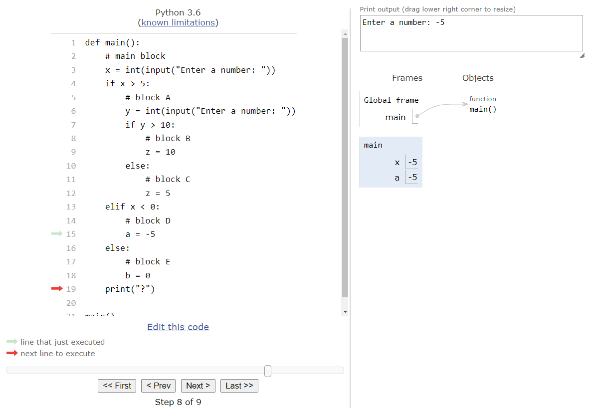
Because of this, we have to be careful when we write our programs in Python using function scope. It is very easy to find ourselves in situations where our program will work most of the time, since it usually executes the correct blocks of code to populate the variables we need, but there may be situations where that isn’t guaranteed.
This is where testing techniques such as path coverage are so important. If we have a set of inputs that achieve path coverage, and we are able to show that the variables we need are available at the end of the program in each of those paths, then we know that we can use them.
Alternatively, we can build our programs in Python as if Python used block scope instead of function scope. By assuming that variables are only available in the blocks where they are given a value, we can always ensure that we won’t reach a situation where we are trying to access a variable that isn’t available. For novice programmers, this is often the simplest option.
Dealing with scope is a tricky part of learning to program. Thankfully, in Python, as well as many other languages, we can easily use tools such as Python Tutor and good testing techniques to make sure our programs are well written and won’t run into any errors related to variable scope.
Let’s go through another worked example to see how we can translate a problem statement into a working program. We’ll also take a look at how we can test the program to verify that it is working as intended.
Here’s a short and simple game that can be played by two players:
Three players each guess a positive integer greater than $0$, and then share them simultaneously. The winner is chosen following this formula:
- If any two players have chosen the same number, the game is a tie.
- If all players have chosen even numbers, or all players have chosen odd numbers, then the smallest number wins.
- Otherwise, the largest number wins.
This game has some similarities to Rock Paper Scissors, but the logic is quite a bit different. So, let’s work through how we would build this program using conditional statements.
Our first step should be to build a simple program that handles user input. So, we’ll create a new Python program that contains a main() function, a call to the main() function, and three variables to store user input. We’ll also use the input() function to read input, and the int() function to convert each input to an integer. Below that, we’ll add some print statements for testing. At this point, our program should look similar to this:
def main():
    p1 = int(input("Enter a positive integer for player 1: "))
    p2 = int(input("Enter a positive integer for player 2: "))
    p3 = int(input("Enter a positive integer for player 3: "))

    # debugging statements
    print("player 1 chose {}".format(p1))
    print("player 2 chose {}".format(p2))
    print("player 3 chose {}".format(p3))


main()
With this code in place, we’ve already created a Python program that we can run and test. So, before moving on, let’s run this program at least once to verify that it works correctly. This will help us quickly detect and correct any initial errors in our program, and make it much easer to debug logic errors later on.
So, when we run this program, we should see output similar to this:
Now that we have confirmed our program is working, let’s start writing the logic in this program. Deciding which conditional statement to write first is a very important step in designing a program, but it is difficult to learn what works best without lots of practice. If we look at the problem statement above, we see that there are several clear conditions that we’ll have to check:
However, there is one more condition that we should also keep in mind. This one isn’t clearly stated in the rules, but implied in the problem statement itself:
So, to write an effective program, we should first make sure that all of the inputs are greater than $0$. We can do this using a simple conditional statement. We’ll also remove our debugging statements, as they are no longer needed:
def main():
    p1 = int(input("Enter a positive integer for player 1: "))
    p2 = int(input("Enter a positive integer for player 2: "))
    p3 = int(input("Enter a positive integer for player 3: "))

    if p1 <= 0 or p2 <= 0 or p3 <= 0:
        print("Error")
    else:
        print("All numbers are greater than 0")


main()
In this conditional statement, we are checking to see if any one of the numbers is less than or equal to $0$. Of course, using some Boolean algebra and De Morgan’s law, we can see that this is equivalent to checking if all numbers are not greater than $0$. Either approach is valid.
Once we know we have valid input, the next step in determining a winner is to first determine if there are any ties. For this, we simply need to check if any two players input the same number. Since there are three players, we need to have three different Boolean expressions to accomplish this. In our program, we could add a conditional statement as shown here:
def main():
    p1 = int(input("Enter a positive integer for player 1: "))
    p2 = int(input("Enter a positive integer for player 2: "))
    p3 = int(input("Enter a positive integer for player 3: "))

    if p1 <= 0 or p2 <= 0 or p3 <= 0:
        print("Error")
    else:
        if p1 == p2 or p2 == p3 or p3 == p1:
            print("Tie")
        else:
            print("Not a Tie")


main()
This is a pretty simple Boolean expression that will check and see if any possible pair of inputs is equal. We use the or Boolean operator here since any one of those can be true in order for the whole game to be a tie.
Next, let’s tackle whether the inputs are all odds or all evens. If we look at the rules above, this seems to be the next most logical thing we’ll need to know in order to determine the winner of the game. Recall that we can determine if a number is even or odd by using the modulo operator % and the number $2$. If that result is $0$, the number is even. If not, the number is odd.
In code, we can express that in a conditional statement as shown here:
def main():
    p1 = int(input("Enter a positive integer for player 1: "))
    p2 = int(input("Enter a positive integer for player 2: "))
    p3 = int(input("Enter a positive integer for player 3: "))

    if p1 <= 0 or p2 <= 0 or p3 <= 0:
        print("Error")
    else:
        if p1 == p2 or p2 == p3 or p3 == p1:
            print("Tie")
        elif p1 % 2 == 0 and p2 % 2 == 0 and p3 % 2 == 0:
            print("All numbers are even")
        elif p1 % 2 != 0 and p2 % 2 != 0 and p3 % 2 != 0:
            print("All numbers are odd")
        else:
            print("Numbers are both even and odd")


main()
Notice that we are using the and Boolean operator in these conditional statements, because we want to be sure that all numbers are either even or odd.
In this example, we’re also choosing to use chained conditional statements with the elif keyword instead of nesting the conditionals. This helps clearly show that each outcome is mutually exclusive from the other outcomes.
However, we chose to nest the program logic inside of the outermost conditional statement, which checks for valid input. This helps us clearly see the part of the program that is determining who wins the game, and the part of the program that is validating the input. Later on, we’ll see how we can rewrite that conditional statement into a loop to prompt the user for new input, so it makes sense for us to keep it separate for now.
Once we know if the numbers are either all even or all odd, we know that the winning number is the smallest number of the three inputs. So, how can we determine which number is the smallest? We can use a couple of nested conditional statements!
Let’s handle the situation where all numbers are even first. We know that the smallest number must be smaller than both other numbers. So, we can use a couple of Boolean expressions to check if that is the case for each number:
def main():
    p1 = int(input("Enter a positive integer for player 1: "))
    p2 = int(input("Enter a positive integer for player 2: "))
    p3 = int(input("Enter a positive integer for player 3: "))

    if p1 <= 0 or p2 <= 0 or p3 <= 0:
        print("Error")
    else:
        if p1 == p2 or p2 == p3 or p3 == p1:
            print("Tie")
        elif p1 % 2 == 0 and p2 % 2 == 0 and p3 % 2 == 0:
            if p1 < p2 and p1 < p3:
                print("Player 1 wins")
            elif p2 < p1 and p2 < p3:
                print("Player 2 wins")
            else:
                print("Player 3 wins")
        elif p1 % 2 != 0 and p2 % 2 != 0 and p3 % 2 != 0:
            print("All numbers are odd")
        else:
            print("Numbers are both even and odd")


main()
Here, we start by checking if player 1’s number is smaller than both player 2’s and player 3’s. If so, then player 1 is the winner. If not, we do the same for player 2’s number. If neither player 1 nor player 2 has the smallest number, then we can assume that player 3 is the winner without even checking.
As it turns out, we would end up using the exact same code in the situation where all numbers are odd, so for now we can just copy and paste that set of conditional statements there as well:
def main():
    p1 = int(input("Enter a positive integer for player 1: "))
    p2 = int(input("Enter a positive integer for player 2: "))
    p3 = int(input("Enter a positive integer for player 3: "))

    if p1 <= 0 or p2 <= 0 or p3 <= 0:
        print("Error")
    else:
        if p1 == p2 or p2 == p3 or p3 == p1:
            print("Tie")
        elif p1 % 2 == 0 and p2 % 2 == 0 and p3 % 2 == 0:
            if p1 < p2 and p1 < p3:
                print("Player 1 wins")
            elif p2 < p1 and p2 < p3:
                print("Player 2 wins")
            else:
                print("Player 3 wins")
        elif p1 % 2 != 0 and p2 % 2 != 0 and p3 % 2 != 0:
            if p1 < p2 and p1 < p3:
                print("Player 1 wins")
            elif p2 < p1 and p2 < p3:
                print("Player 2 wins")
            else:
                print("Player 3 wins")
        else:
            print("Numbers are both even and odd")


main()
That covers the situations where all players have input either even or odd numbers. We can quickly test this program a couple of times by providing various inputs that match those cases. So, when we run this program, we should see output like this:
However, as soon as we do that, we should start thinking about ways to simplify this program. This is because we are using the same exact code in multiple places in our program, which goes against one of the key principles of writing good programs: Don’t Repeat Yourself! .
Anytime we see this happen, we should start thinking of ways to move that code into a new function. This is actually really easy to do in this case: we can simply write a function named smallest() that accepts three numbers as input, representing the three player’s guesses, and then it can print the winning player for us. So, let’s update our program to include a new function, and then call that function from within our conditional statement:
def smallest(p1, p2, p3):
    if p1 < p2 and p1 < p3:
        print("Player 1 wins")
    elif p2 < p1 and p2 < p3:
        print("Player 2 wins")
    else:
        print("Player 3 wins")


def main():
    p1 = int(input("Enter a positive integer for player 1: "))
    p2 = int(input("Enter a positive integer for player 2: "))
    p3 = int(input("Enter a positive integer for player 3: "))

    if p1 <= 0 or p2 <= 0 or p3 <= 0:
        print("Error")
    else:
        if p1 == p2 or p2 == p3 or p3 == p1:
            print("Tie")
        elif p1 % 2 == 0 and p2 % 2 == 0 and p3 % 2 == 0:
            smallest(p1, p2, p3)
        elif p1 % 2 != 0 and p2 % 2 != 0 and p3 % 2 != 0:
            smallest(p1, p2, p3)
        else:
            print("Numbers are both even and odd")


main()
By using the same variable names as the parameters for the smallest() function, we can easily just copy/paste the conditional statement from the main() function into the smallest() function without making any changes to it. We already know it works, so we shouldn’t change it if we don’t have to.
Once again, now is a great time to test this program and make sure that everything is working before moving on.
The last step is to determine the largest number in the case that the numbers are not all even or odd. Since we’ve already written a function named smallest() to handle the opposite, let’s quickly write another function named largest() to handle this case. We can then call that function in the False branch of our conditional statement handling the logic of the program:
def smallest(p1, p2, p3):
    if p1 < p2 and p1 < p3:
        print("Player 1 wins")
    elif p2 < p1 and p2 < p3:
        print("Player 2 wins")
    else:
        print("Player 3 wins")


def largest(p1, p2, p3):
    if p1 > p2 and p1 > p3:
        print("Player 1 wins")
    elif p2 > p1 and p2 > p3:
        print("Player 2 wins")
    else:
        print("Player 3 wins")


def main():
    p1 = int(input("Enter a positive integer for player 1: "))
    p2 = int(input("Enter a positive integer for player 2: "))
    p3 = int(input("Enter a positive integer for player 3: "))

    if p1 <= 0 or p2 <= 0 or p3 <= 0:
        print("Error")
    else:
        if p1 == p2 or p2 == p3 or p3 == p1:
            print("Tie")
        elif p1 % 2 == 0 and p2 % 2 == 0 and p3 % 2 == 0:
            smallest(p1, p2, p3)
        elif p1 % 2 != 0 and p2 % 2 != 0 and p3 % 2 != 0:
            smallest(p1, p2, p3)
        else:
            largest(p1, p2, p3)


main()
There we go! We’ve written a complete program that implements the problem statement given above. Did you think it would end up being this complex? Sometimes even a simple problem statement ends up requiring quite a bit of code to implement it fully.
The next step is to perform some testing of our program to make sure it is fully working. To do that, we need to come up with a set of inputs that would achieve branch coverage, and possibly even path coverage. However, this time our program is spread across three functions, so it makes it a bit more difficult to do. So, let’s focus on each individual function separately and see if we can find a set that work for each of them.
First, we see the main function has 5 branches to cover, so we need to come up with 5 different sets of inputs in order to achieve branch coverage. We can keep the inputs very small, just to make our testing a bit simpler. Here are the 5 branches to cover, and an input that will reach each one:
-1, -1, -11, 1, 12, 4, 61, 3, 51, 2, 3Notice how we are trying to come up with the simplest possible inputs for each branch? That will make it easier to combine these inputs with the ones used in other functions to find an overall set of inputs that will achieve branch coverage for the entire program.
Next, we can look at the function to find the smallest number. This function is called when the inputs are either all even or all odd. So, we know that either inputs 2, 4, 6 or 1, 3, 5 will call this function.
Within the function itself, we see three branches, depending on which player wins. So, if we start with the input 2, 4, 6, we’ll see that this will execute the branch where player 1 wins. To execute the other branches, we can simply reorder the inputs:
2, 4, 64, 2, 64, 6, 2That will achieve branch coverage for the smallest() function, and even overlaps with one of the inputs used in the main() function.
The same applies to the function to find the largest number, but in this case we need a mix of even and odd numbers in the input. So, the input 1, 2, 3 will execute this function, and that input results in player 3 winning. Once again, we can reorder that input a bit to execute all three branches of this function:
3, 1, 21, 3, 21, 2, 3Therefore, based on our analysis, we can achieve branch coverage across the entire program using 9 different inputs:
-1, -1, -11, 1, 12, 4, 64, 2, 64, 6, 21, 3, 53, 1, 21, 3, 21, 2, 3This will execute each branch of all conditional statements in the program at least once.
Once we’ve achieved branch coverage, we should also quickly look at path coverage: is there any possible pathway through this program that we haven’t tested yet? As it turns out, there are two, but they are somewhat difficult to find. Can you spot them? See if you can figure it out before continuing on in this page.
The paths we missed are situations where the numbers are all odd, but a player other than player 1 wins. While we tested all possible branches in the smallest() function, we didn’t test it using all odd numbers more than once. So, to truly achieve path coverage, we should add two more inputs to our list above:
-1, -1, -11, 1, 12, 4, 64, 2, 64, 6, 21, 3, 53, 1, 53, 5, 13, 1, 21, 3, 21, 2, 3So, with a total of 11 inputs, we can finally say we’ve achieved both branch coverage and path coverage of this program.
In this lab, we introduced several major important topics in Python. Let’s quickly review them.
Conditional statements are mutually exclusive when only one of the many branches will be executed for any possible input.
if condition_1:
    print("1")
else
    if condition_2:
        print("2")
    else:
        if condition_3:
            print("3")
        else:
            print("4")
is equivalent to:
if condition_1:
    print("1")
elif condition_2:
    print("2")
elif condition_3:
    print("3")
else:
print("4")if condition_1:
if condition_2:
print("1 and 2")
elif condition_3:
print("1 and 3")
else:
print("1 and not 2 or 3")
elif condition_4:
if condition_2:
print("4 and 2")
elif condition_3:
print("4 and 3")
else:
print("4 and not 2 or 3")
else:
print("neither 1 nor 4")Variable scope refers to what parts of the code a particular variable is accessible in. Python uses function scope, which means that a variable defined anywhere in a function is available below that definition in any part of the same function.
Other languages use block scope, where variables are only available within the block where they are defined.
The first type of loop we’ll explore in pseudocode is the while loop. A while loop is an iteration statement that will constantly repeat the code inside of it while a Boolean expression evaluates to true. This is very similar to how an if statement is constructed - we know that the code inside an if statement is only executed if the associated Boolean expression is true. In the case of a while loop, we do basically the same thing, but at the end of the code inside the loop, we go back to the top and check the Boolean expression again. If it is still true, then we execute the code inside it over and over until it evaluates to false.
In pseudocode, the basic structure of a while loop is shown here:
REPEAT WHILE(<boolean expression>)
{
    <block of statements>
}
When we encounter a while loop, we first evaluate the <boolean expression> inside the parentheses to see if it is true. If so, we enter the loop and execute all of the code in the <block of statements> between the curly braces {}. Once we’ve reached the end of the block, where the closing curly brace } is found, we then go back to the top and evaluate the <boolean expression> again. If it evaluates to true, we run the code inside the loop again.
We keep doing this until the <boolean expression> evaluates to false. As soon as it does, we jump down to the code immediately following the closing curly brace } at the end of the loop - we don’t execute the code inside the loop again.
This also means that when we initially reach the loop, we could run into the situation where the <boolean expression> evaluates to false the first time we see it. In that case, we just jump to the end of the loop and start executing the code after the closing curly brace }. There is no guarantee that we’ll ever execute the code inside the loop, just like in an if statement.
To understand how a while loop works in practice, let’s code trace an example program. Consider the pseudocode program shown here:
PROCEDURE main()
{
    DISPLAY("Enter a number: ")
    x <- NUMBER(INPUT())
    y <- 1
    REPEAT WHILE(y <= x / 2)
    {
        IF(x MOD y = 0)
        {
            DISPLAY(x + " is divisible by " + y + "\n")
        }
        y <- y + 1
    }
}

main()
Before we run a code trace on this program, take a moment to read it and see if you can guess what it does!
As always, we’ll start our code trace by reviewing the code and keeping track of variables and procedures, as well as output. So, our initial setup will look like this:
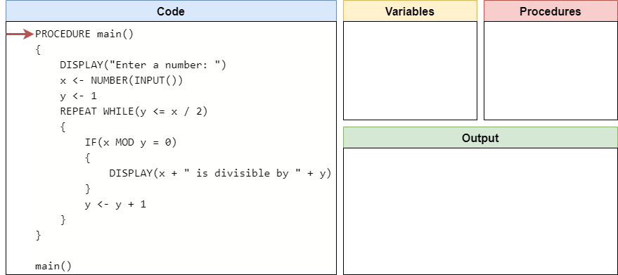
As we scan through the program, we’ll find the main() procedure and record it in our list of procedures.
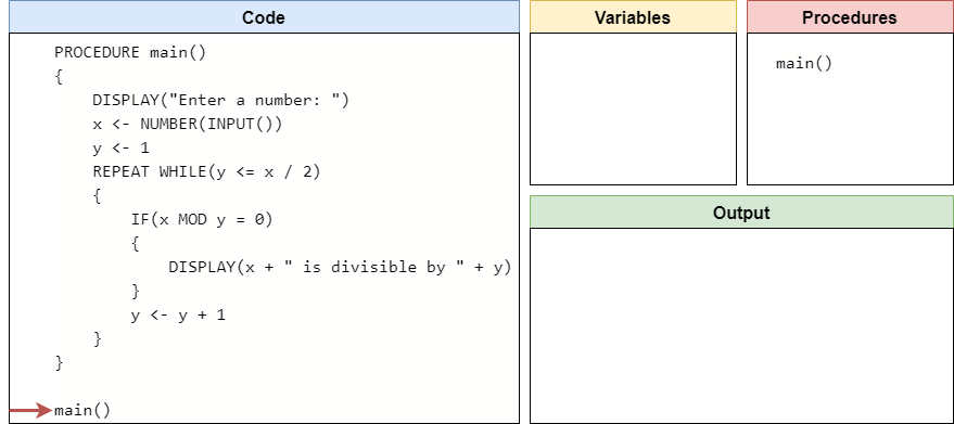
At the bottom of the program, we’ll find a call to the main() procedure, so we’ll jump to that procedure’s code and start executing it.
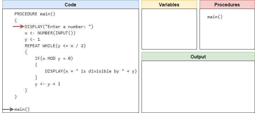
The first two lines of the main() procedure simply prompt the user for input and then store that input in the variable x. In this example, let’s assume the user inputs the string "12" as input. So, we’ll store the number $12$ in the variable x
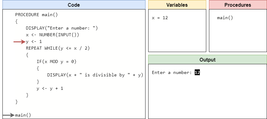
Next, we’ll store the value $1$ in the variable y.
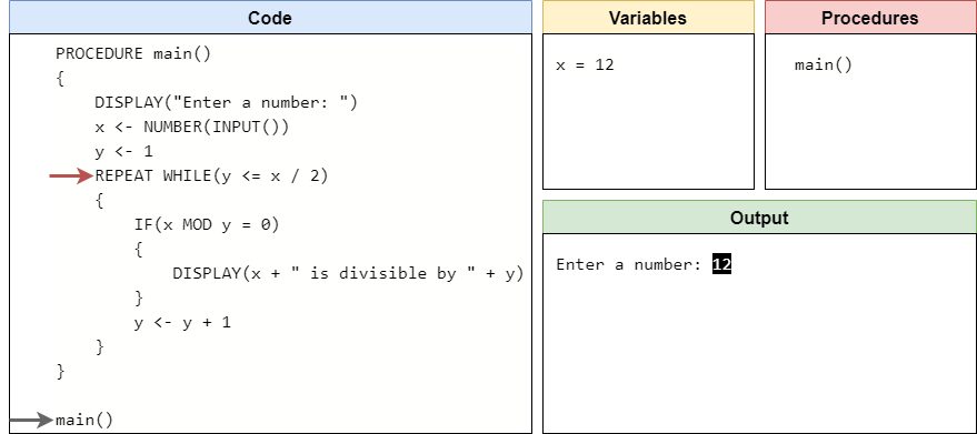
At this point, we’ve reached the start of our loop. So, first we need to determine if the Boolean expression inside of the parentheses is true or false. Looking at the expression, it is checking if the value in y is less than or equal to half of the value stored in x. Since x is currently storing $12$, we know that half of x is $6$. Because y is only storing $1$, we know that y is definitely less than or equal to $6$, and the Boolean expression evaluates to true. Therefore, we should enter the loop and start executing the code inside.
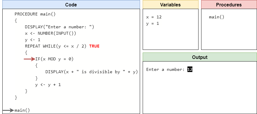
Inside of the loop, we find an if statement. So, we must determine if the Boolean expression inside of the if statement is true as well. In this case, we are checking if the remainder of dividing x by y is $0$ using the MOD operator. This is the same as checking to see if x can be evenly divided by y. Since y is currently $1$, we know that any integer divided by $1$ is itself with no remainder. So, this Boolean expression will evaluate to true and we should execute the code inside the if statement.
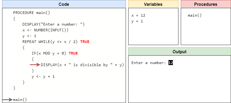
Here, we find a DISPLAY() statement, so we’ll just add that to our output and then exit the if statement below.

Below the if statement, we see a simple assignment statement that will increase, or increment, the value of y by $1$. So, the variable y is now storing the value $2$.
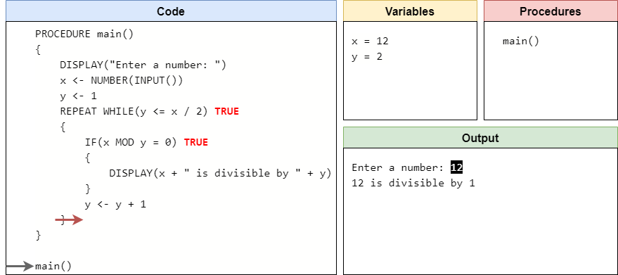
At this point, we’ve reached the end of the while loop. So, we need to loop back up to the beginning of the loop and start over again.
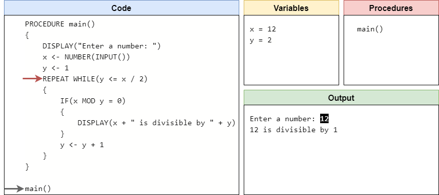
Here, we need to once again evaluate the Boolean expression inside of the while loop. Since the value of y has changed, it might be different this time. However, we see that the $2$ store in y is still less than or equal to half of the value $12$ stored in x, so we enter the loop again.

Inside the loop, we repeat the same process as before. We start by evaluating the Boolean expression inside of the if statement. Since $12$ is evenly divisible by $2$, that expression is true and we should enter the if statement.
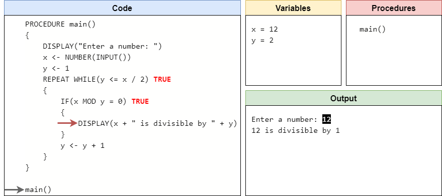
So, once again we’ll print some output to the terminal:
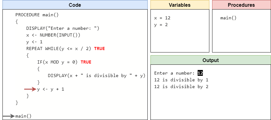
And then we’ll leave the if statement and increment the value stored in y by $1$.
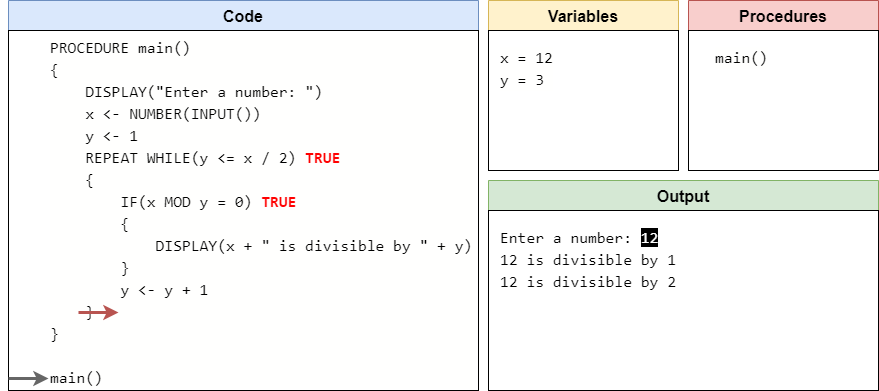
We’re at the bottom of the loop, so we’ll need to repeat by going back to the top once again.
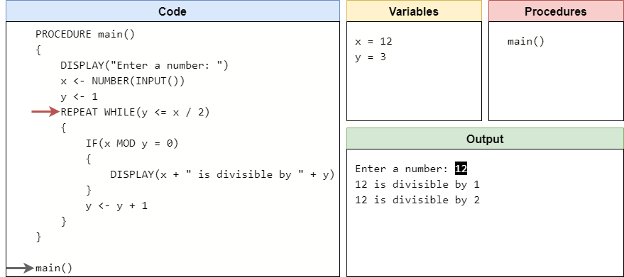
Hopefully by this point we have a pretty good idea of how this loop is working. We first check to see that $3$ stored in y is less than or equal to half of the value in x. Since it is, we’ll continue the loop, and in the if statement inside we’ll find that $12$ is evenly divisible by $3$, so we’ll print some output, increment y by $1$, and loop back to the top. So, after that whole iteration, we should see the following in our code trace:
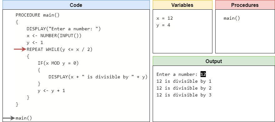
With small, simple loops like this one, once we know what it does, we can typically just treat the whole loop like a single statement in our mental model of a computer. We know that it will increment the value of y each time, and if the value of x is equally divisible by y, it will print some output. Finally, we know we should keep repeating this step until y is greater than half the value of x. In many cases, we can simply refer to each iteration of the loop by the values of the variables used in the loop itself. So, after the iteration where y is equal to $4$, we’ll see this state:

Likewise, after the iteration where y is $5$, we’ll see this state:
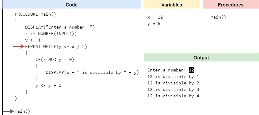
Notice that this iteration did not produce any output, since $12$ is not evenly divisible by $5$. At this point, y is storing the value of $6$. Since that is exactly half of $12$, it still makes the Boolean expression true so we should execute the code in the loop again. After that iteration, we’ll see the following state:
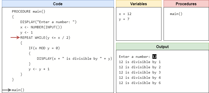
At this point, y is now storing the value $7$. Since $7$ is not less than or equal to half of $12$, the Boolean expression inside the while loop will evaluate to false and we’ll jump down to the bottom of the loop.
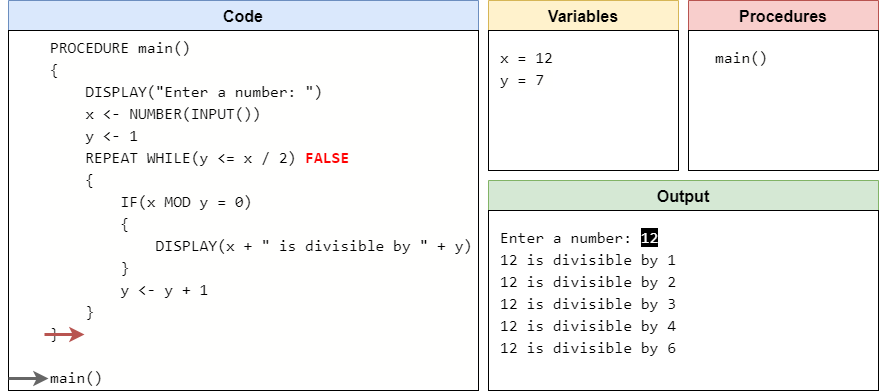
Since there is no more code in the main() procedure, we’ll return back to where the procedure was called, and then we’ll see that we’re at the end of the program! An entire trace of the program is shown in this animation.
As we can see, this program will determine all of the possible factors of the value that is provided by the user as input, and it will print them one at a time to the output.
Another way to visualize a while loop is using a flowchart. The pseudocode program above can be represented as the following flowchart:

In this flowchart, we once again begin at the top at the circle labeled “Start”. From there, we see that our program will read input and store it in the variable x. We also create the variable y and store the initial value of $1$ there. At this point, we hit a diamond-shaped decision node, representing the while loop. If the Boolean expression in that decision node is true, then we follow the branch to the right that enters the loop. Here, we see yet another decision node that represents the if statement inside of the loop. When we see a loop and an if statement side by side in a flowchart like this, it is very easy to see how similar they actually are.
After the if statement, we increment the value stored in y, and then we see the flowchart path will loop back up to the beginning of the while loop, starting with the decision node at the top. This is the key concept in a while loop - once we reach the end of an iteration, we must go back to the top and enter the decision node once again.
When we reach a point where the Boolean expression evaluates to false, our flowchart will then finish at the circle labeled “End”.
So, just like we saw with conditional statements, using flowcharts is another great way we can try to understand the control flow in our programs. Feel free to make use of any of these tools as we continue to develop more complex programs in this course.
In the Official AP Pseudocode
, the REPEAT WHILE loop is instead replaced with a REPEAT UNTIL loop. The concept is the same, except that the loop will repeat until the Boolean expression is true, instead of while the Boolean expression is true. We feel it is worth highlighting this change, since it does deviate from the official standard.
This is a very subtle change, and it is easy to translate between the two by simply adding a Boolean NOT operator to the Boolean expression. However, we chose to introduce loops using REPEAT WHILE instead of REPEAT UNTIL because most programming languages, including Python, only use while loops. There are few, if any, modern languages that use an “until” loop, and we feel that it adds an unnecessary complication to our pseudocode language. So, we’ve chosen to stick more closely to Python’s loop structures than the ones introduced in the AP Pseudocode.
Another type of loop that is commonly used in programming is the for loop. Instead of a while loop, which only uses a Boolean expression to determine if a loop repeats, a for loop is typically used to iterate a defined number of times, either by counting up or by iterating across a data structure such as a list. We’ll learn more about how to use for loops with lists later in this course.
In pseudocode, a for loop is used to iterate a specific number of times. The basic syntax for a for loop is shown here:
REPEAT <n> TIMES
{
    <block of statements>
}
In this example, the placeholder <n> is used to represent a number, typically a positive integer, that gives the number of times the loop should be executed. Then, we will execute the statements in the <block of statements> the given number of times. Put another way, we can say that this loop will execute the <block of statements> for n times - this is why we call this a for loop.
Let’s look at a quick example program to see how a for loop works in practice. Consider the following pseudocode program:
PROCEDURE main()
{
    DISPLAY("Enter a number: ")
    x <- NUMBER(INPUT())
    DISPLAY("Enter a number: ")
    y <- NUMBER(INPUT())
    z <- 1
    REPEAT y TIMES
    {
        z < z * x
    }
    DISPLAY(x " to the power of " y " = " z)
}

main()
Just like before, take a minute to read this program and see if you can determine how it works before continuing to the description below.
Once again, we’ll begin by setting up or code tracing structure as shown here:
First, we’ll find the main() procedure, and record it in the list of procedures.
Then, we’ll encounter a call to the main() procedure, so we’ll move our execution to the first line of code inside of that procedure.
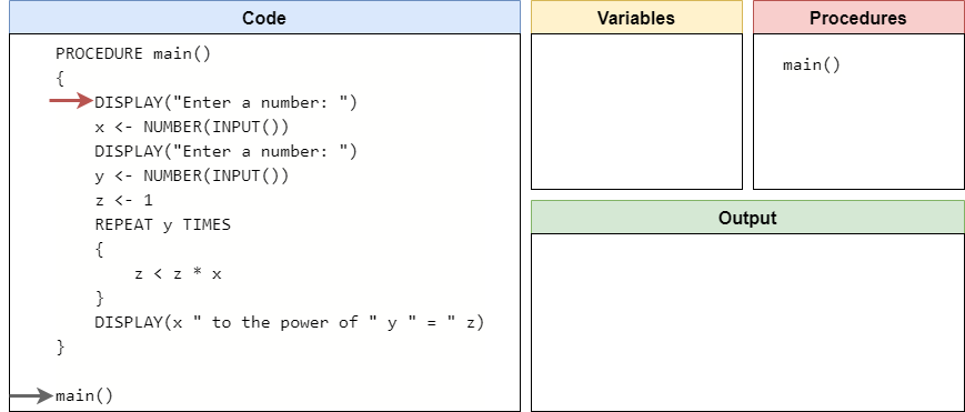
Here, the first two lines will prompt the user to input a number, and then that number will be stored in the variable x. For this example, let’s assume the user inputs the string "5", so the number $5$ will be stored in the variable x.
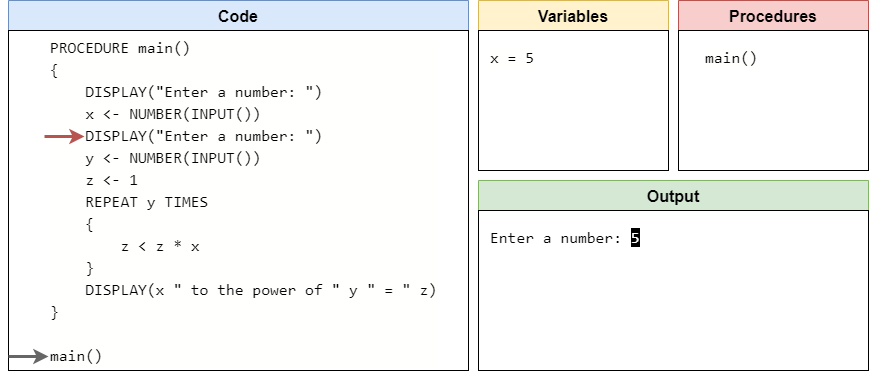
Likewise, we’ll do the same for the variable y. So, let’s assume the user inputs "3", which will store the number $3$ in the variable y.
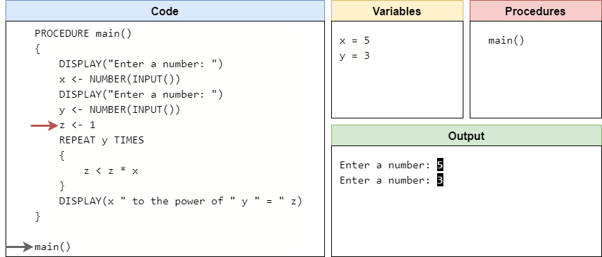
The program will also initialize the variable z by storing the number $1$ in it.

At this point, we’ve reached the for loop in our code. When we evaluate a for loop, we need to keep track of how many iterations are left. So, the easiest way to do that is to create a new hidden variable that is initially set to the value given for how many times to repeat the loop, and then we can count down using that variable. So, in our list of variables, we’ll create a new variable i to keep track of the loop. It should initially store the same value that is stored in y, so we’ll store $3$ in i.
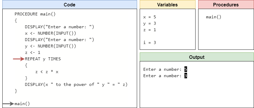
Now we are ready to see if we should enter the loop. Since i is greater than $0$, we know that we have at least one loop iteration to go. Therefore, we’ll enter the loop.
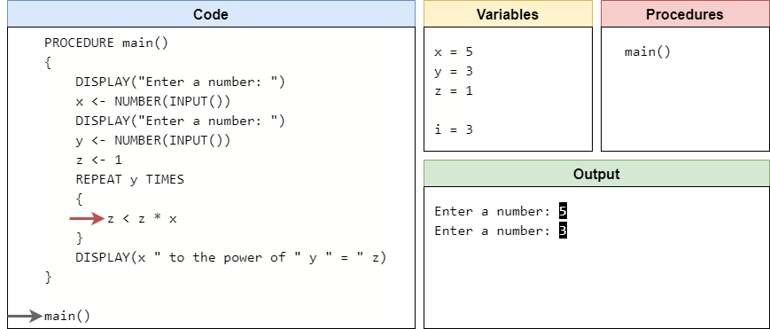
Inside the loop, we’ll update the value stored in z by multiplying it by x. So, z will now store the value $5$.

Now we’ve reached the end of the loop. At this point, we’ve completed a full iteration of the loop, so we can subtract $1$ from the hidden loop counter variable i. This is called decrementing a variable. Once we’ve done that, we can loop back up to the beginning of the loop itself.

Here, we once again must check to see if we should enter the loop. Since our loop counter variable i is greater than $0$, we know that we can enter the loop again.

Inside the loop, we’ll once again update the value in z by multiplying it by x. So, z now stores $25$.

Then, we’ll reach the end of the loop, so we must decrement the value in i and jump back to the top of the loop.
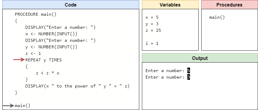
Since i is still greater than $0$, we’ll enter the loop once again.

We’ll multiply the value in z by x, which means z will now be storing $125$.
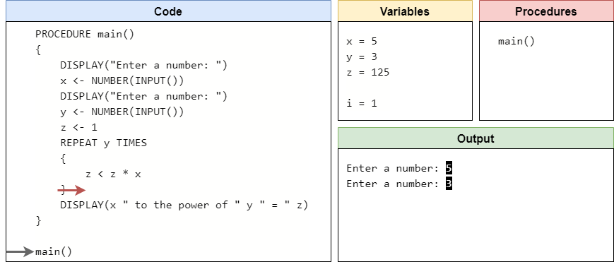
At the end of the loop, we’ll decrement i again and return back to the top of the loop.

At this point, we see that i is now equal to $0$. This means that we’ve executed the loop the correct number of times, we can now jump to the code after the loop.
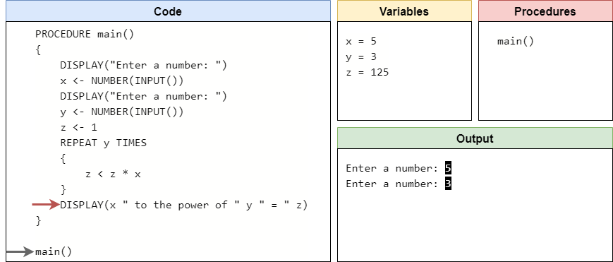
Finally, at the end of the program, we’ll print the result of our calculation.
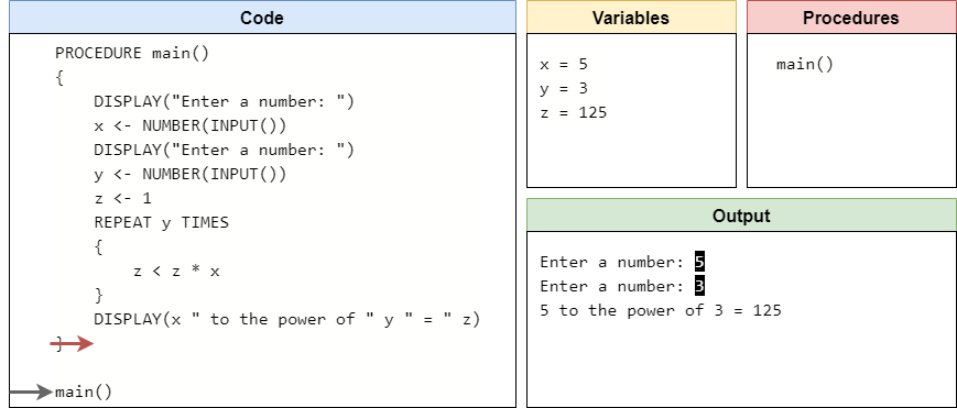
Now that we’ve reached the end of the main() procedure, we’ll return back to where it was called from. Since that is the end of the code, the program stops executing. A full animation of this program can be seen here.
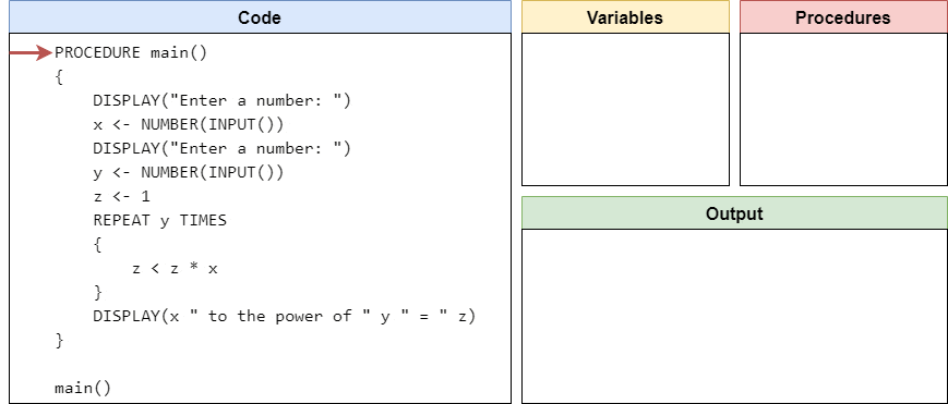
As we were able to show through code tracing, this program will compute the result of taking the first input to the power of the second input. Since the power operation is simply repeatedly performing multiplication a set number of times, it is easily done through the use of a for loop.
One of the most powerful features of loops is to deal with invalid user input. For example, if we want a user to input a positive number, but they accidentally input a negative number instead, what should our program do? Previously, all we could do was print an error and ask the user to run the program again, but that isn’t very user friendly or efficient. Instead, we can use a loop to repeatedly prompt the user for input until we receive a valid input.
Let’s look at an example to see how this works. Consider the following pseudocode procedure:
PROCEDURE positive_input()
{
    DISPLAY("Enter a positive number: ")
    x <- NUMBER(INPUT())
    REPEAT WHILE(x <= 0)
    {
        DISPLAY("Invalid Input!\n")
        DISPLAY("Enter a positive number: ")
        x <- NUMBER(INPUT())
    }
    RETURN x
}
This procedure will prompt the user for input, and then store whatever is received in the variable x. However, if the user inputs a number that is less than or equal to $0$, it will print an error message and prompt the user for input once again. Let’s quickly code trace through this procedure to see how it works.
When code tracing a procedure, we simply start as if we are calling the procedure from somewhere else. So, our setup will look like this:
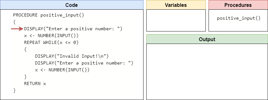
This program begins by prompting the user for input, and then storing the input as a number in the variable x. So, let’s assume that the user input the string "-5" when prompted. So, that will store the value $-5$ in the variable x.
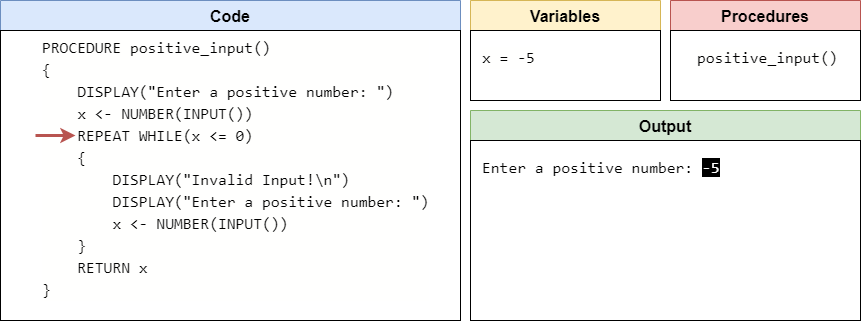
At this point, we’ve reached the beginning of our loop, so we need to determine if the Boolean expression evaluates to true or false. Since the value stored in x is less than or equal to $0$, the Boolean expression is true and we should enter the loop.
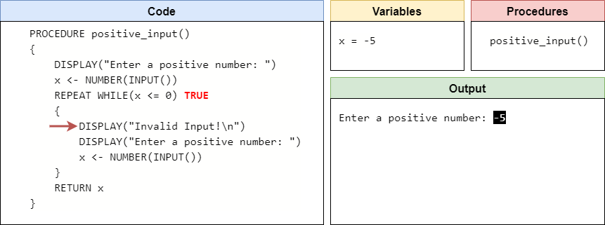
Inside the loop, we know that the most recent input from the user was invalid. So, we’ll print an error message, followed by a new prompt for input, and then we can read a new value from the user. This time, let’s assume the user has input the string "0", so we’ll store the value $0$ in the variable x.
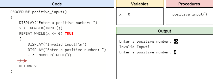
Now we’ve reached the end of the loop, so we must go back to the beginning of the loop and start over.

Here, we can check the Boolean expression once again. Since x now stores the value $0$, it is still less than or equal to $0$, so we should enter the loop again.
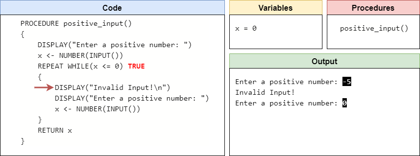
Just like before, we’ll print an error and then prompt the user for new input. This time, let’s assume the user inputs the string "7", so we’ll store the value $7$ in the variable x.
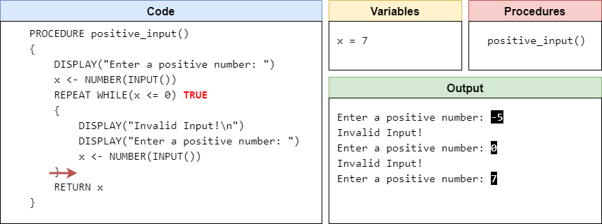
We’re at the end of the loop once again, so now we’ll jump back to the beginning of the loop.
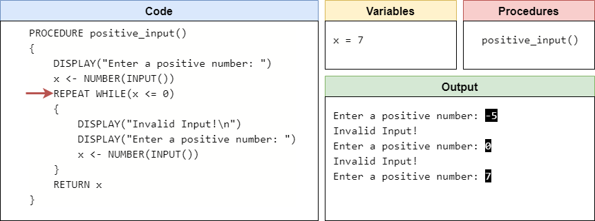
Here, we can test the Boolean expression yet again. This time, however, since x is not less than or equal to $0$, the Boolean expression is false and we can jump past the loop.
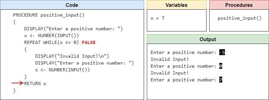
At the bottom of the procedure, we are returning the value we received as input from the user. So, the value returned by this procedure will be $7$, which is a valid input that we received from the user itself. A full animation of this procedure is shown here.
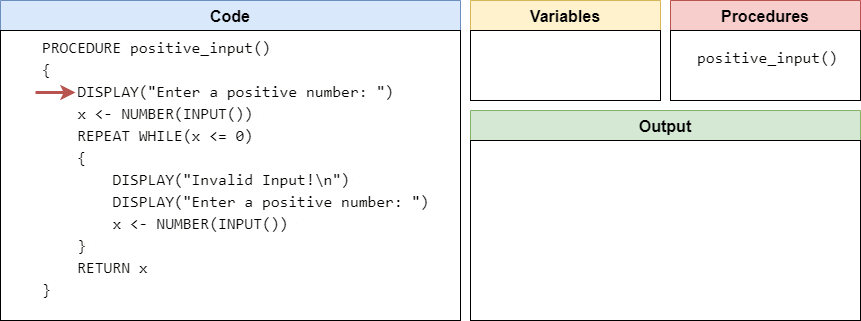
Once we’ve created a procedure such as this in our programs, we can easily use it to read input from the user and verify that it meets the requirements we need. For example, consider this main() procedure that uses the positive_input() procedure we created above:
PROCEDURE main()
{
    a <- positive_input()
    b <- positive_input()
    c <- (a + b) / 2
    DISPLAY("The midpoint is " + c)
}
This program will simply find the midpoint between two positive numbers. All of the code for handling user input is in the positive_input() procedure, and we can call it multiple times to get multiple different inputs from the user.
The positive_input() procedure is a great example of a simple design pattern that is commonly used in programs. A design pattern is simply a structure in code that is used to solve a particular problem, usually one that comes up often in many different programs. If we learn to solve these little problems by using these common programming structures, or patterns, it makes it much easier for others to read and understand our code. In addition, by learning these design patterns ourselves, it makes it much easier for us to solve common problems in our code - we can simply apply the relevant design pattern instead of trying to create a new solution from scratch. So, feel free to make use of the positive_input() procedure shown here, or adapt it as needed, anytime you need to read input from a user.
Now that we’ve seen many examples of how to use loops in our code, let’s briefly discuss some techniques for testing programs that contain loops. Many of these techniques are similar to ones we’ve explored when testing conditional statements, but there are a few important nuances to think about.
First, just like we explored with conditional statements, it is important to test our programs in a way that we execute every possible branch, and try to find every possible path through the program as well. When dealing with a loop, usually we just consider two paths - one where the loop is entered at least once, and one where the loop is skipped entirely, if possible.
Consider this example program in pseudocode:
PROCEDURE main()
{
    x <- NUMBER(INPUT())
    y <- NUMBER(INPUT())
    REPEAT WHILE(x < y)
    {
        x = x + x
    }
    DISPLAY(x)
}
This program will repeatedly double x until it larger than y. So, let’s come up with some inputs for this program that achieve branch and path coverage.
To achieve branch coverage, we must simply come up with a set of inputs that will execute every line of code in the procedure at least once. So, let’s try inputting $3$ and $5$ first. Since x is less than y, we enter the loop at least once. Eventually, x will become greater than y, so we’ll exit the loop as well at some point. Therefore, we can say that the inputs 3 and 5 are enough to achieve branch coverage.
In this sample program, we’ve already executed all of the code, but we may want to try and come up with a set of inputs that will bypass the loop completely. This helps us check to make sure there aren’t any issues with the code if the loop isn’t executed at all. For this instance, consider the inputs 5 and 3. In this case, the value in x is already greater than y, so the program will never execute the code inside of the loop at all. Thankfully, this doesn’t break anything, so we know this program will work just fine without executing the loop.
When testing code that contains a loop, there is one other test we must consider - is it possible to reach a situation where the loop will never terminate? That is, once we start executing code within the loop, is it possible to get stuck in the loop and then never actually complete the program?
Therefore, we must think carefully about our loops and situations that might cause problems. For example, what if we provide the inputs -5 and -3 to the pseudocode program above?
In that case, we’ll enter the loop since $-5$ is less than $-3$, but once we’ve executed the code in the loop, we’ll see that x is now storing $-10$! We’ve actually gotten further away from a situation where the loop will terminate, which is definitely not good. In fact, this loop will repeat infinitely, and our program will run forever.
So, we should either rethink our program a bit, or possibly add additional code to make sure the user does not input a negative value for y. By properly testing our program, we were able to discover a situation where the loop would not terminate!
Unfortunately, it can be difficult to definitively prove if a loop will terminate in all cases. In computer science, we typically use a special concept known as a loop variant in order to prove that a loop will eventually terminate. Loosely, a loop variant is a way of expressing a maximum number of possible iterations of a loop before it terminates based on the current state of the program.
In the example above, we could say that our loop variant is the difference between x and y. Then, as long as we can show that the difference between those two values is monotonically decreasing each time the loop iterates, we can show that eventually it will reach a $0$ or less than $0$ and the loop will terminate. If the loop variant does not decrease, then the loop will not terminate.
In this course, you won’t be expected to reach that level of detail, but hopefully you’ll be able to use some simple logic and common sense to figure out if a loop will terminate or if there are situations where it won’t work correctly.
Let’s go through a complete worked example program so we can see how to use loops to transform a problem statement into a working program. Once we’re done, we’ll also talk about how we can test the program to determine if it works correctly and won’t run into an error.
For this example, we’re going to write a simple program to play a variant of the game Nim known as the 21 Game . Here are the rules:
The game begins with the first player choosing either $1$, $2$, or $3$. Then, the second player chooses either $1$, $2$ or $3$ and adds that number to the number chosen by the first player to establish a total. The game continues by alternating between players, each choosing to add either $1$, $2$ or $3$ to the total. The game is over when the total reaches $21$ or higher. The player who adds the number to the total that causes the game to end is the loser.
This is a very simple game, and a great example of how loops can be used in a program in a variety of different ways. So, let’s see what it takes to create this program.
To begin, we need to start with a main() procedure and a call to the main() procedure, as shown here:
PROCEDURE main()
{

}

main()
Next, we know that the program will repeat until the total is greater than or equal to $21$. So, we can easily add a variable to keep track of the total, and a loop that will represent the actual game being played.
PROCEDURE main()
{
    total <- 0
    REPEAT WHILE(total <= 21)
    {
        # players take turns
    }
    # game over
}

main()
We also need some way to keep track of which player’s turn it is. So, we’ll need a variable to track that, as well as a simple conditional statement at the end of our loop to switch between the two players. In pseudocode, that would look like this:
PROCEDURE main()
{
    total <- 0
    player <- 1
    REPEAT WHILE(total <= 21)
    {
        # player's turn
        IF(player = 1)
        {
            player = 2
        }
        ELSE
        {
            player = 1
        }
    }
    # game over
}

main()
As we can see, we just use a variable that switches between the values $1$ and $2$ to keep track of the current player. At the end of the loop, we have a conditional statement that checks the current value of that variable, and then switches it to the other value. This allows our players to take turns within a single loop.
Next, we need a way for our players to provide input. Thankfully, earlier in this lab we saw a simple procedure for accepting input from a user and checking to make sure it is valid. So, we can simply borrow that procedure and tweak it a little bit to fit this scenario. Here is what that procedure would look like in pseudocode:
PROCEDURE read_input(player)
{
    DISPLAY("Enter 1, 2, or 3 for player " + player + ": ")
    x <- INPUT()
    REPEAT WHILE(x != "1" AND x != "2" AND x != "3")
    {
        DISPLAY("Invalid Input!\n")
        DISPLAY("Enter 1, 2, or 3 for player " + player + ": ")
        x <- INPUT()
    }
    RETURN NUMBER(x)
}
This procedure is a bit different than the previous one because it requires a parameter. The parameter is used to represent the current player, and we include that in the prompt for input to show which player’s turn it is. Without that, the game would be very confusing. We’ve also updated the Boolean expression inside of the while loop to make sure the value input is either "1", "2", or "3". If it isn’t, it will print an error message and prompt the same player for input again. Once a valid input has been received, it will return that value back to where this procedure was called from.
Unfortunately, in pseudocode, there isn’t a good way to require users to input whole numbers. For this example, the number of possible inputs is small enough that it makes the most sense to just check for the individual string values themselves, and then convert the input to a number once it has been verified. There are many other approaches in both pseudocode and Python that will achieve the same result.
Now that we have a procedure for handling input, we must simply add that procedure call to our main() procedure, and use it to update the value stored in the total. We can also add a message at the end to determine which player is the winner. The final, complete program is shown here:
PROCEDURE read_input(player)
{
    DISPLAY("Enter 1, 2, or 3 for player " + player + ": ")
    x <- INPUT()
    REPEAT WHILE(x != "1" AND x != "2" AND x != "3")
    {
        DISPLAY("Invalid Input!\n")
        DISPLAY("Enter 1, 2, or 3 for player " + player + ": ")
        x <- INPUT()
    }
    RETURN NUMBER(x)
}

PROCEDURE main()
{
    total <- 0
    player <- 1
    REPEAT WHILE(total <= 21)
    {
        # player's turn
        total <- total + read_input(player)
        IF(player = 1)
        {
            player = 2
        }
        ELSE
        {
            player = 1
        }
    }
    # game over
    DISPLAY("Player " + player + " wins!")
}

main()
Notice at the end of the main() procedure that we are able to print the player that wins, instead of the losing player. This is because we are switching between players at the end of the while loop, so once the total reaches a value greater than or equal to $21$, we know that we’ve already switched the player variable to be the other player, instead of the one that just caused the game to end. It’s a subtle logic choice, but it works well in this case.
Take a moment to work through this program and make sure you understand how it works. We won’t do a full code trace, but you are welcome to do so to make sure you are comfortable with it before continuing.
Now that we’ve written our program, let’s test it to see if it works correctly. Testing this program is a bit different than some of the other programs we’ve created, mainly because it heavily restricts the inputs that are valid. Each player can only input the strings "1", "2", or "3" as valid input. Any other string is invalid, and will result in the loop inside of the read_input() procedure repeating.
Therefore, when testing our program, we should make sure we try each of these inputs, but also try some invalid inputs as well. The order the inputs are provided also matters - for path coverage, we want to test the situation where a valid input is provided first and the loop in read_input() is skipped, and also the situation where a valid input is provided after an invalid input or two, so the loop in read_input() is executed.
Finally, since this program will read inputs many times while it is executing, we can’t simply use multiple sets of inputs. Instead, we have to look at entire lists of inputs, where the order that they are provided matters as much as the inputs themselves.
Consider the following list of inputs, which are marked with the player’s turn and the updated sum or error:
| Input | Player | Sum/Error |
|---|---|---|
"1" |
1 | 1 |
"2" |
2 | 3 |
"3" |
1 | 6 |
"0" |
2 | error |
"4" |
2 | error |
"1" |
2 | 7 |
"-1" |
1 | error |
"5" |
1 | error |
"2" |
1 | 9 |
"lizard" |
2 | error |
"(*&#$&*^@" |
2 | error |
"3" |
2 | 12 |
"invalid" |
1 | error |
"3" |
1 | 15 |
"broken" |
2 | error |
"2" |
2 | 17 |
" " |
1 | error |
"1" |
1 | 18 |
"3" |
2 | 21 |
| Player 1 Wins |
This list represents one complete game. The first input, "1", will be the first input provided by player 1, then the "2" will be player 2’s turn, and so on. However, as the inputs progress, we start to see some invalid inputs as well. When the game receives an invalid input, the read_input() procedure will enter the loop, and the same player will be prompted for input again until a valid input is received. So, looking through this list, we see that it includes both the situation where the input provided is valid the first time, bypassing the loop, as well as situations where the initial input provided by a player is invalid, entering the loop and prompting for additional input. So, this set of input achieves path coverage in just one game!
We may also want to test and make sure that it is possible for both players to win. To do that, we can simply come up with another set of inputs similar to the one given above, but use different values for the valid inputs to make sure that player 2 wins that game. By doing so, we’ve achieved every possible outcome of the game.
The other part of testing this program is to show that the loops will terminate properly. You won’t be required to prove this yourself in this course, but you should still think about it when designing and testing them. So, let’s briefly take a look at that process as well.
First, we can look at the loop in read_input() procedure. This is a bit tricky, since the condition for repeating in the loop is entirely driven by user input. So, we really can’t say whether the loop will terminate or not, but we can easily show that if the user inputs a valid value, the loop will correctly terminate and the program can continue running. So, as far as our testing goes, that’s good enough.
The loop in the main() procedure is a bit different. This loop will repeat while the value stored in total is less than or equal to $21$. So, to prove this loop will terminate, we need to come up with a loop variant and show that it is reducing each time the loop is executed. Thankfully, we can just say that the loop variant is 21 - total. As the value in total increases, that value will decrease until it reaches $0$ or less.
To show that it is constantly decreasing, we can simply say that the read_input() procedure will always return a positive integer, and that value is added to the total each time the loop iterates. So, since total is always getting larger, the loop variant is getting smaller, and the loop will eventually terminate.
There we go! That’s a complete worked example for building and testing a program that contains multiple loops in different procedures. Hopefully this is helpful as you move ahead to the next part of the lab, where you are asked to create and test your own programs. Good luck!
In this lab, we introduced several major important topics in pseudocode. Let’s quickly review them.
While loops in pseudocode will execute while a Boolean expression evaluates to true.
REPEAT WHILE(<boolean expression>)
{
    <block of statements>
}For loops in pseudocode will execute a set number of times.
REPEAT <n> TIMES
{
    <block of statements>
}Loops can be used to request new input from the user if invalid input is received.
PROCEDURE positive_input()
{
    DISPLAY("Enter a positive number: ")
    x <- NUMBER(INPUT())
    REPEAT WHILE(x <= 0)
    {
        DISPLAY("Invalid Input!\n")
        DISPLAY("Enter a positive number: ")
        x <- NUMBER(INPUT())
    }
    RETURN x
}Loops can be tested for both branch and path coverage. In general, achieving path coverage involves writing code that will enter the loop, and also code that will bypass the loop entirely.
Loops should also be tested for termination and situations that may result in infinite loops. Using a loop variant and showing that it is monotonically decreasing is a helpful technique.
The first type of loop to explore in Python is the while loop. A while loop uses a Boolean expression, and will repeat the code inside of the loop as long as the Boolean expression evaluates to True. These loops are typically used when we want to repeat some steps, but we aren’t sure exactly how many times it must be done. Instead, we typically know that there is some condition that must be True while we repeat the code, and once it turns False we can stop looping and continue with the program.
The general syntax for a while loop in Python is shown here:
while <boolean expression>:
    <block of statements>
Notice that this syntax is very similar to an if statement. We start with the keyword while, followed by some sort of a <boolean expression> that will evaluate to either True or False. The Boolean expression in Python does not need to be placed inside of parentheses, unlike in pseudocode. After the Boolean expression is a single colon :. Then, starting on the next line and indented one level is a <block of statements> that will be executed when the Boolean expression evaluates to True. Once again, just like in an if statement, we know which statements are part of the block within a while loop based solely on indentation.
Just like in pseudocode, it is possible for the Boolean expression to evaluate to False initially, which will bypass the loop entirely and never execute the code inside of it. Likewise, if we aren’t careful, we can also write a loop where the Boolean expression will always be True, and the loop will run infinitely, causing our program to lock up and never terminate.
To truly understand how a while loop works in Python, let’s go through a simple code tracing example in Python Tutor. Consider the following Python program:
def main():
    x = int(input("Enter a number from 0 to 100: "))
    total = 0
    while total % 100 != x:
        total = total + 9
    print("The smallest multiple of 9 that ends in {} is {}".format(x, total))


main()
See if you can figure out what this program does before moving on!
As always, you can copy and paste this code in the tutor.py file in Codio, or click this Python Tutor
link.
When we load this code in Python Tutor, we should see the usual default state:

The first couple of steps will simply find the main() method and record it in the global frame, and then call the main() method from the bottom of the program
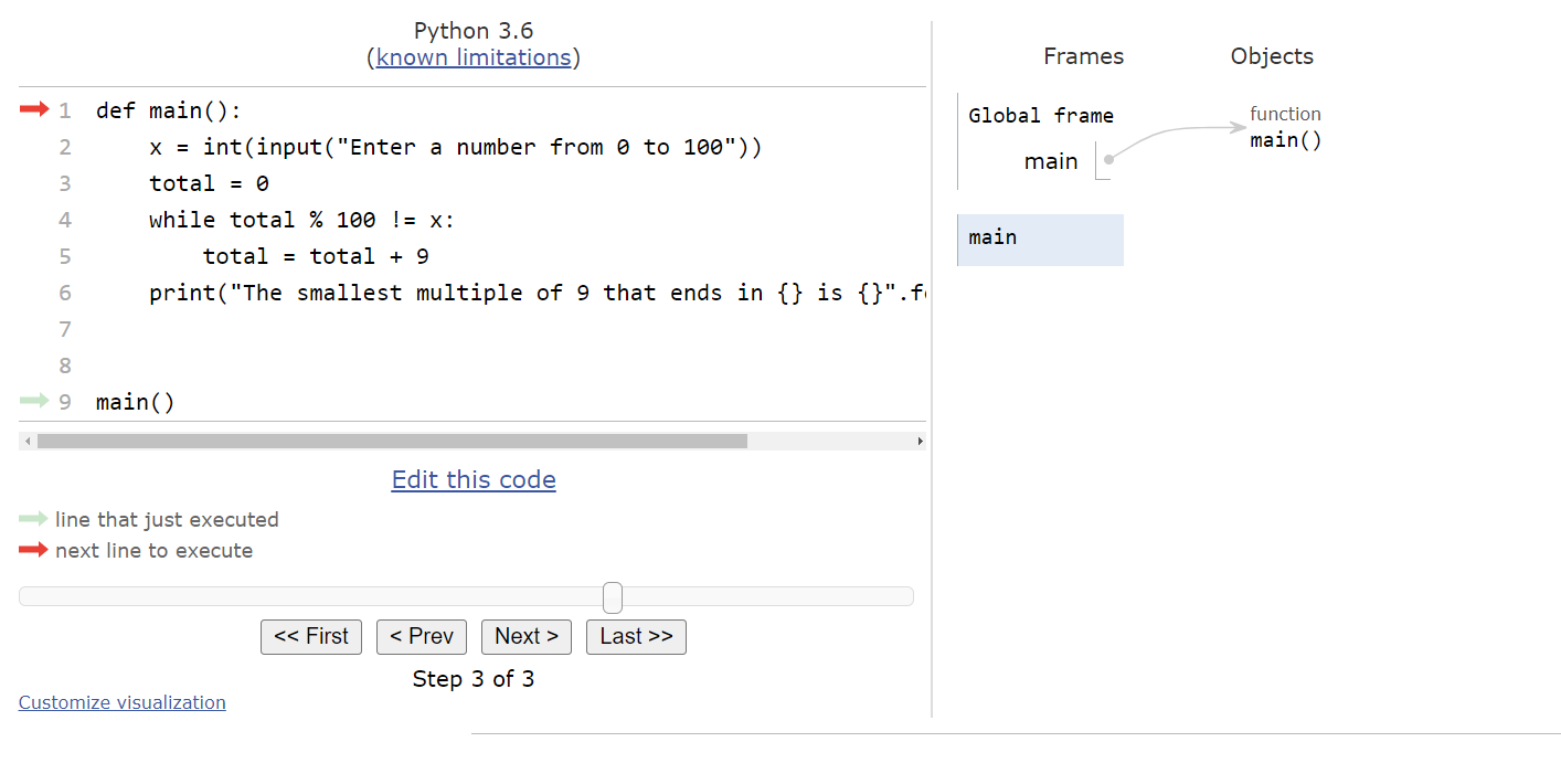
The first line of the program will prompt the user for input and store it in the variable x. For this example, let’s assume the user inputs the string "27".
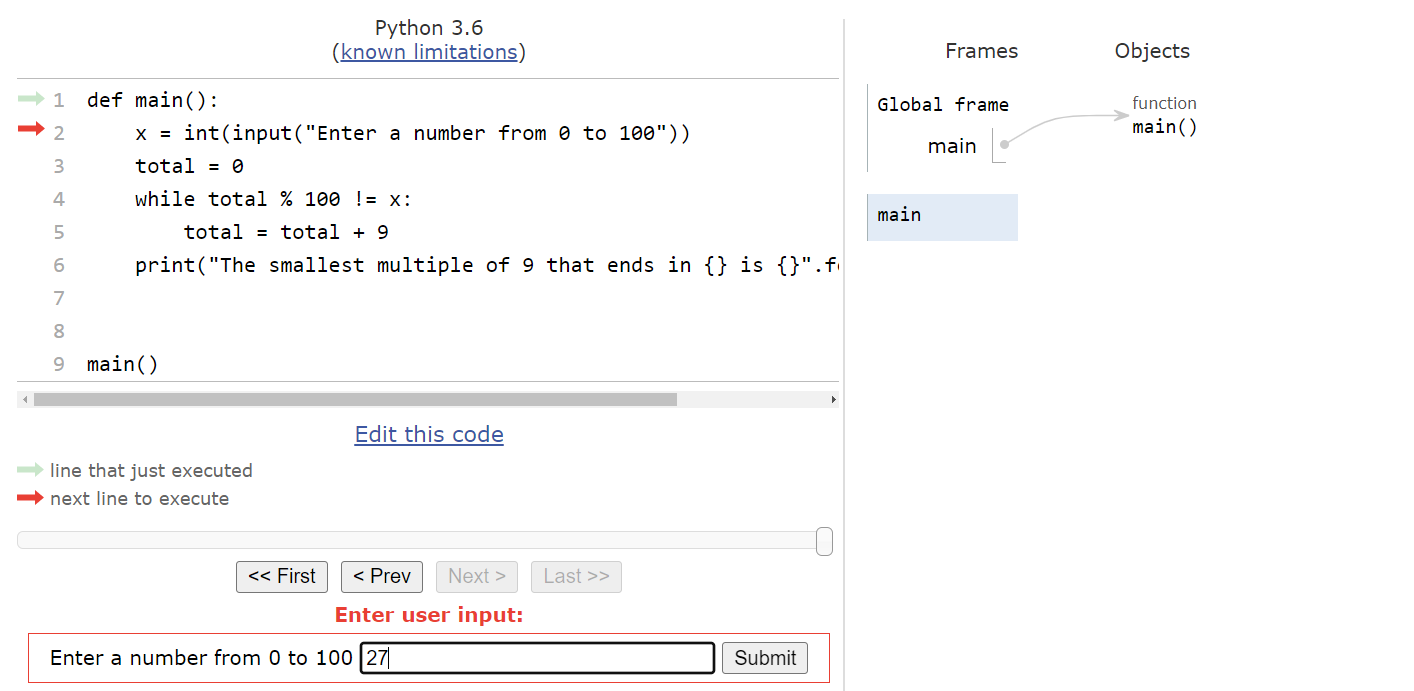
Therefore, we’ll store the value $27$ in the variable x. The next line will store the value $0$ in the variable total, as shown here:
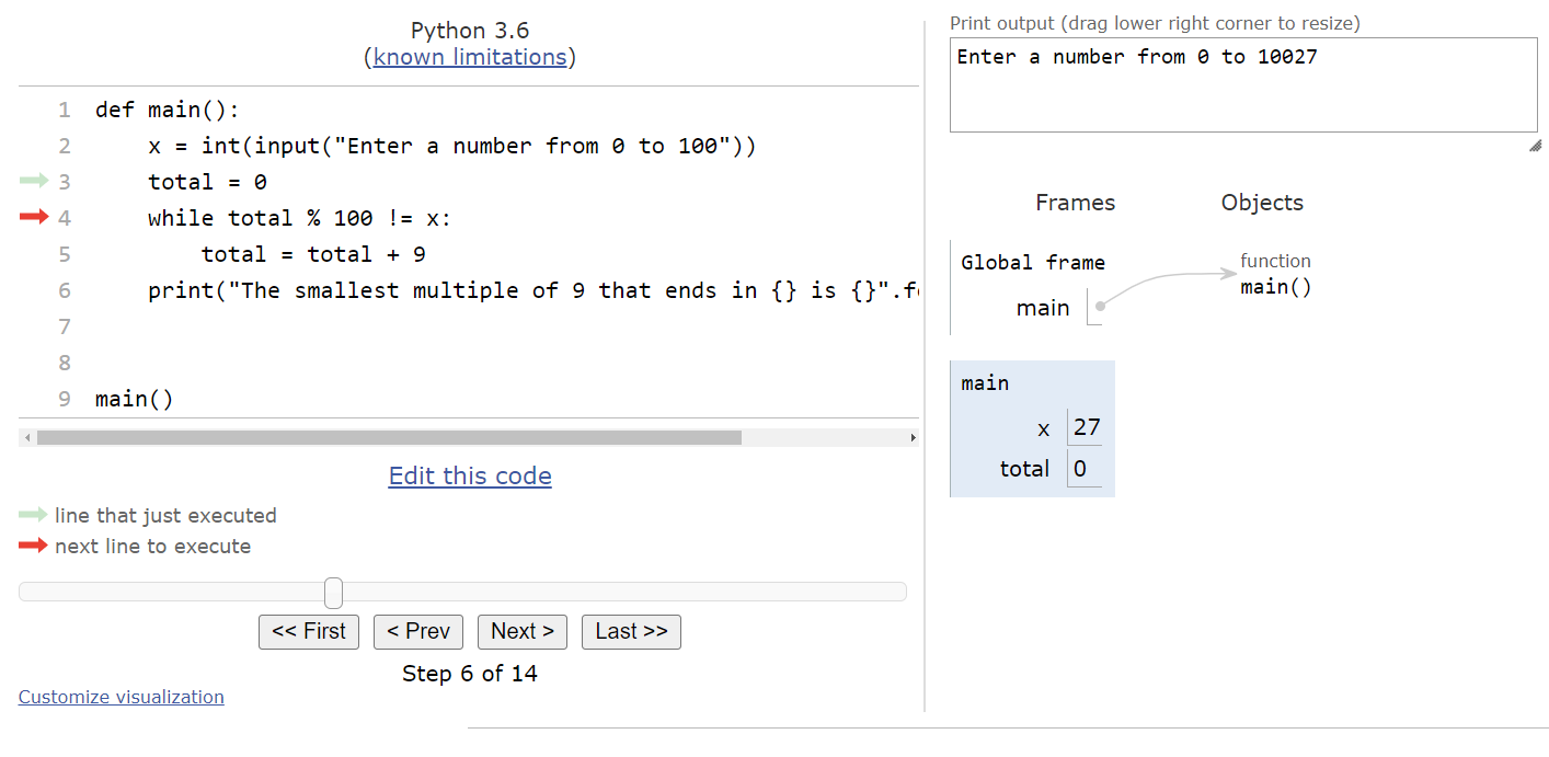
At this point, we’ve reached the beginning of the while loop. So, we’ll need to determine if the Boolean expression evaluates to True or False. In this case, the value of total % 100 is equal to $0$, so it is not equal to the value stored in x. Therefore, the Boolean expression is True, and we should enter the loop.

Inside of the loop, we are simply adding $9$ to the value in total. So, we’ll see that variable is updated, and the execution pointer goes back to the top of the loop.
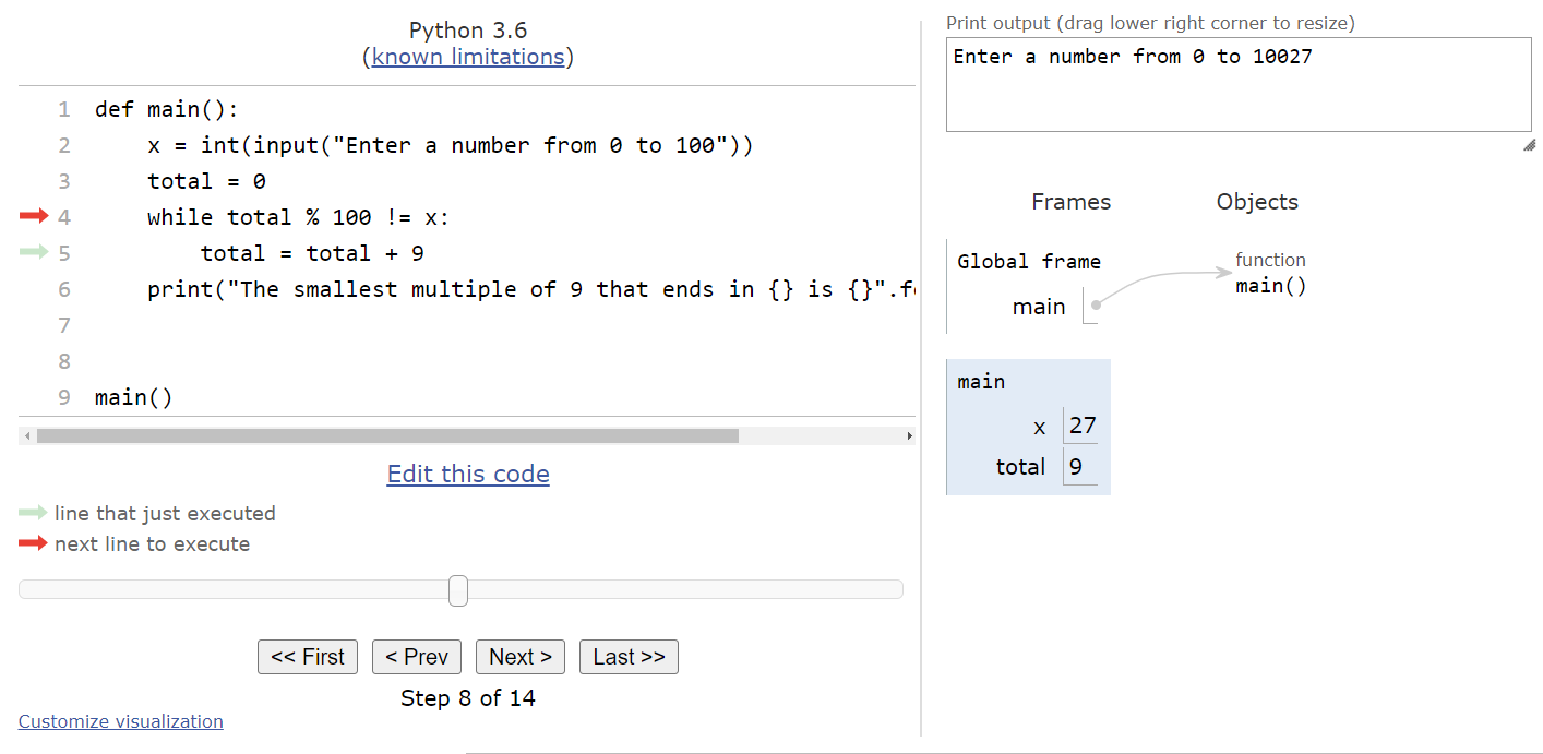
Now that we are back at the top of the loop, we need to check the Boolean expression again. This time the value of total % 100 is $9$, which still isn’t equal to the value stored in x, so we’ll enter the loop again.

We’ll add $9$ to the total here, and jump to the top again.

Once again, we will check the Boolean expression and see that it is still True, so we’ll enter the loop and add $9$ to the total yet again before repeating the process from the top of the loop. At this point, we should see this state in Python tutor.

When we compute total % 100, we get the value $27$, which is the same as the value stored in x. This will make the Boolean expression evaluate to False, so we can skip the loop and jump to the bottom of the program.
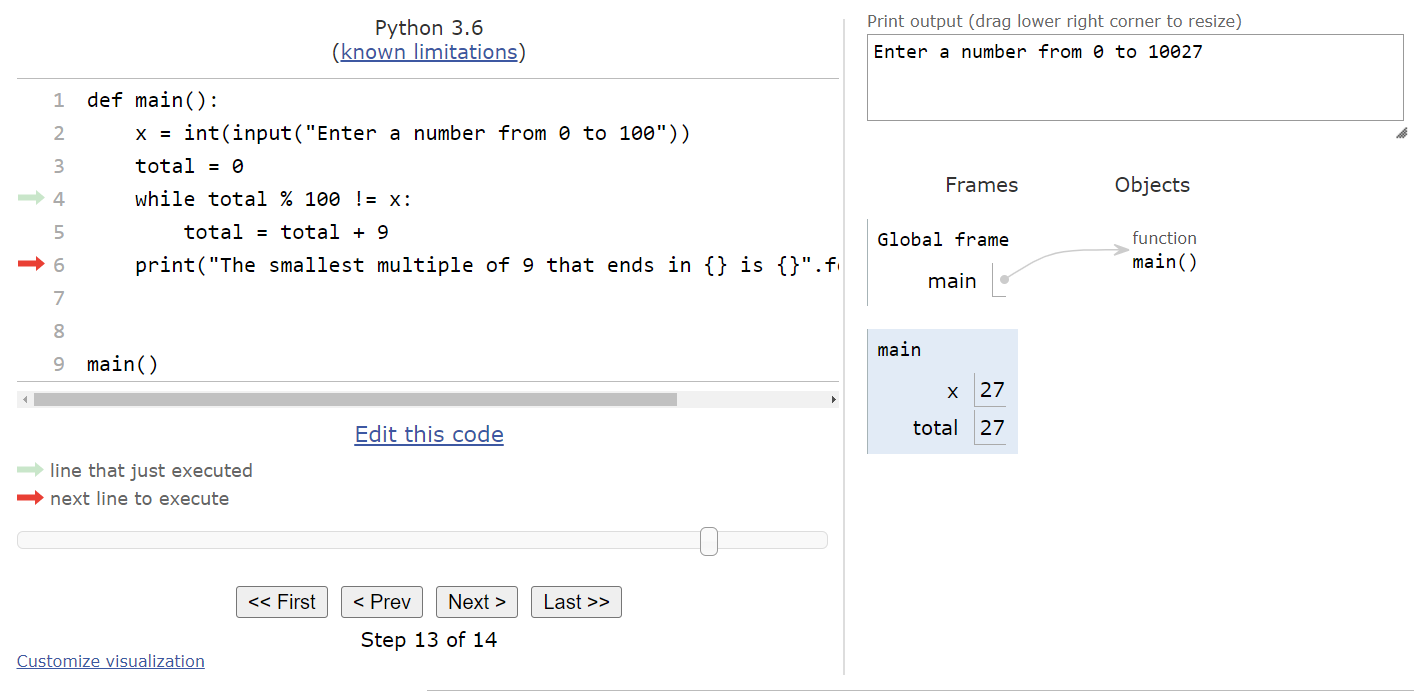
Here, we are simply printing out the output, and then the program will terminate.
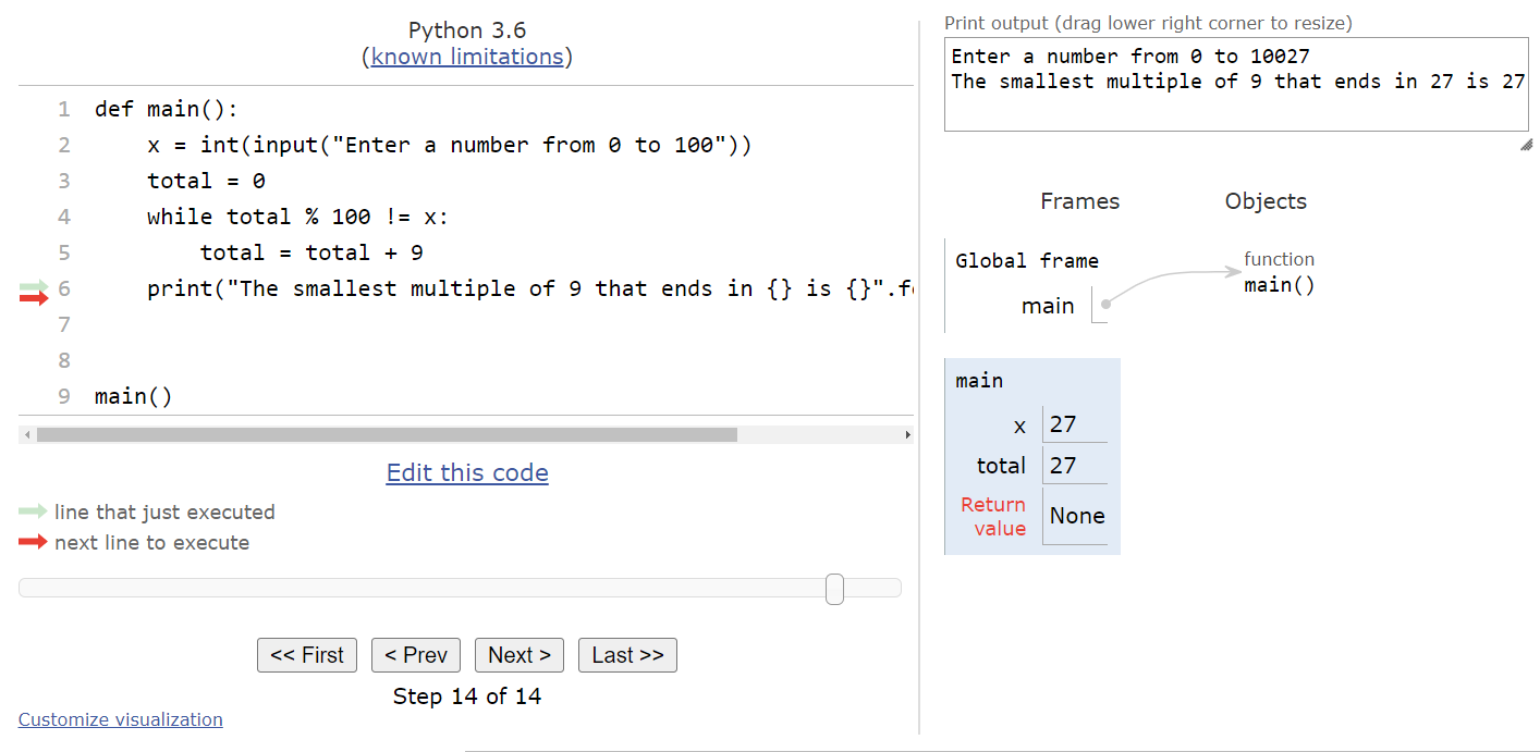
A full animation of this program’s execution in Python Tutor is shown here.
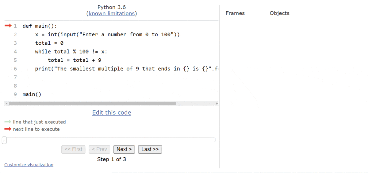
Tracing the execution of a while loop is quite simple, especially with tools such as Python Tutor to help us make sure we’re updating the variables in the correct order.
Python also includes a second type of loop that is very useful, the for loop. Just like in pseudocode, a for loop is used when we want to repeat the steps a certain number of times. However, in Python, we can’t just say that we want to repeat something $10$ times. Instead, we use the built-in range() function in Python to generate a list of numbers that we use in our loop. Then, our for loop will repeat once for each number in the list, and we can even access that number using an iterator variable
We’ll learn more about lists in Python in a later lab. For now, we’re just going to use the range() function to generate them for use with for loops.
The range() function can be used in three different ways, depending on the number of arguments given when calling the function:
range(stop) - with a single argument, the range() function will generate a list of numbers that begins at $0$ and stops before it reaches the stop value. For example, range(10) will generate a list of numbers from $0$ through $9$. This is great, since there will be $10$ numbers in total, so a for loop using range(10) will repeat $10$ times.range(start, stop) - with two arguments, the range() function will generate a list of numbers that begins at start and stops before it reaches the stop value. So, range(3,8) will generate the list [3, 4, 5, 6, 7]. There will be stop - start numbers in the range.range(start, stop, step) - with three arguments, the range() function will generate a list of numbers that begins at start, increases by step each time, and stops before the stop value. Therefore, range(0, 10, 2) will generate the list [0, 2, 4, 6, 8]. We can also use a negative value for step to count backwards. So, range(5, 0, -1) will generate the list [5, 4, 3, 2, 1].You can read more about the Python range() function in the Python Documentation
The general structure of a for loop in Python is shown here:
for <iterator variable> in <list>:
    <block of statements>
The first time we reach a for loop, we’ll keep track of the <list> that we’ll be iterating over. In general, once you start repeating in a for loop, the <list> cannot be changed.
If the list contains at least one item, then we’ll store the first item in the list in the <iterator variable> and enter the for loop to execute the code in the <block of statements> When we reach the end of the block, we’ll jump back to the top and check to see if the <list> contains another item. If so, we’ll store that item in the <iterator variable> and execute the code in the <block of statements> again.
This process will repeat until we’ve used every item in the <list>. Then, we’ll jump to the end of the for loop and continue the program from there.
To really see how a for loop works in Python, let’s use Python Tutor to trace through a quick sample program. Consider this Python program:
def main():
    x = int(input("Enter a number: "))
    line = ""
    for i in range(x):
        line = line + "*"
        print(line)


main()
Before working through the code in Python Tutor, see if you can determine what this program does just by reading it!
To step through the code, we can load it into Python Tutor by placing it in the tutor.py file in the python folder on Codio, or clicking this Python Tutor
link.
We’ll start with the usual default state as shown here:
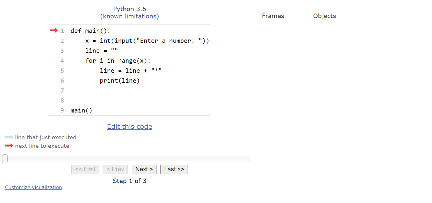
The next two steps will find the main() function in the code and store it in the global frame, and then it will find the main() function call at the bottom of the file. So, once it enters the main() function, we should be at this state:
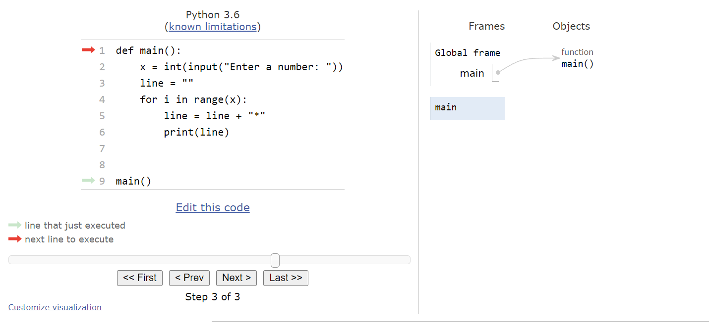
The next line will read the input from the user. For this example, let’s assume the user inputs the string "5":
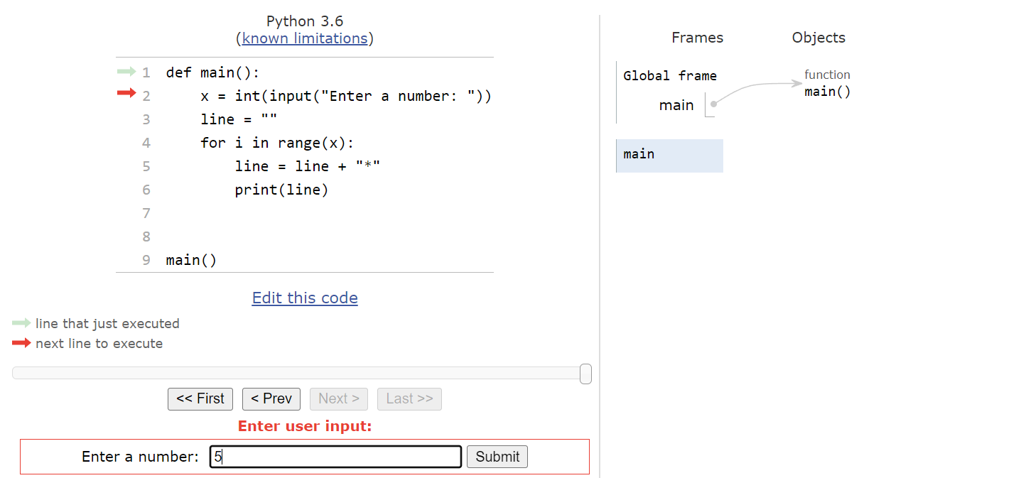
This means that we’ll store the number $5$ in the variable x. The program will also create an empty string value in the line variable, which we’ll use to generate output. At that point, we should have reached the beginning of the for loop.
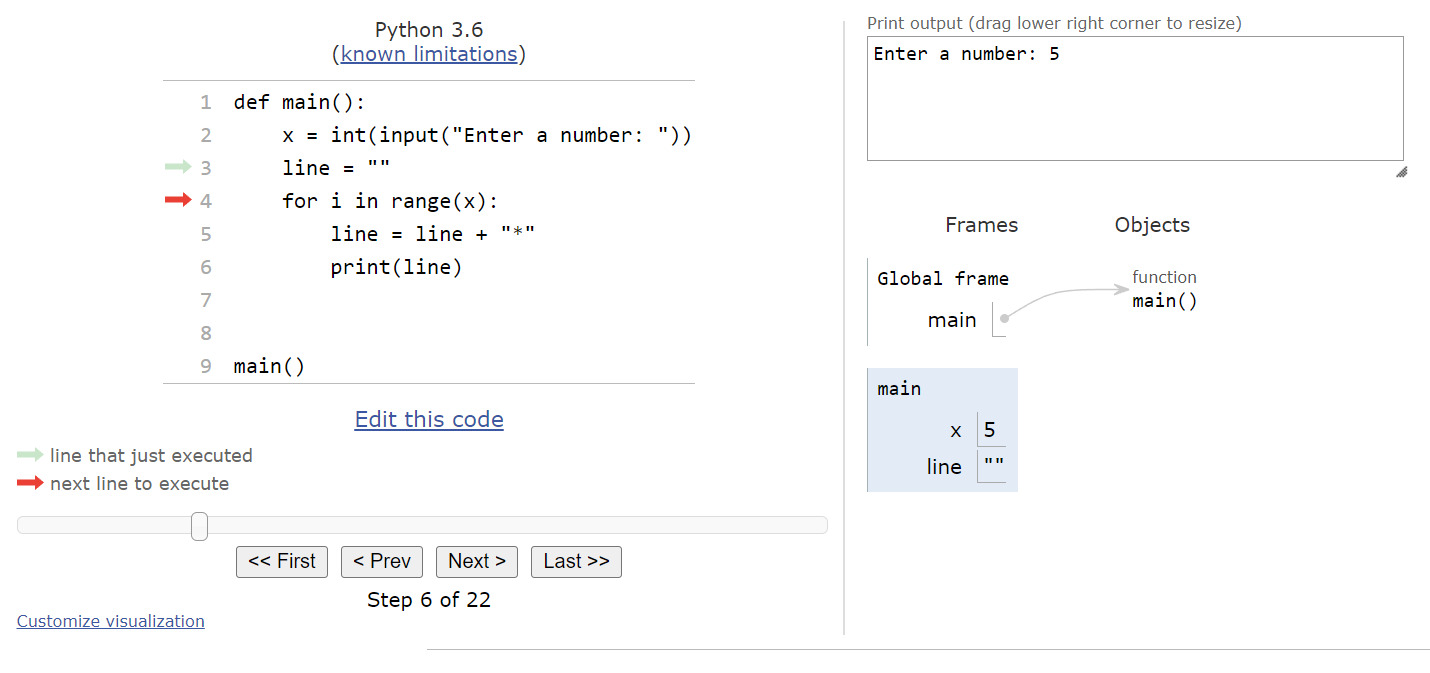
Behind the scenes, Python will generate a list of numbers based on the range() function. Since the range() function is called with a single argument, we know it will be a list of numbers starting at $0$ and ending before it reaches the value in x, which is $5$. So, the list will contain the numbers [0, 1, 2, 3, 4], and it will cause the for loop to repeat $5$ times. For the first iteration of the loop, Python will store the first number in the list, $0$, in the iterator variable i. In programming, we typically use the variable name i to represent our iterator variable. So, once the program has entered the loop, we should see this state:

Inside of the loop, the first statement will update the line value by adding an asterisk * to the end of the string. So, after this statement is executed, the line variable will store a string containing a single asterisk.

The second statement will print the line variable to the output.

At this point, we’ve reached the end of the for loop, so our execution pointer jumps back up to the top of the loop. Then, we check to see if the list we are iterating through contains more values. Again, this list isn’t shown in Python tutor, so we have to mentally keep track, but we can see the current value in i, and we know what the list contains by looking at the range() function. So, we’ll update i to store the value $1$, and repeat the loop once again.
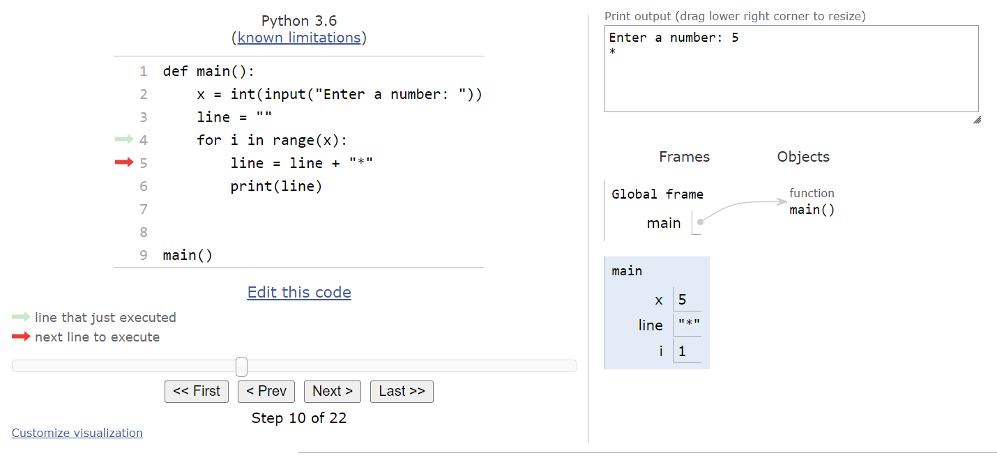
Just like before, this iteration will add an asterisk to the string in the line variable, and then print that to the output before repeating once again.
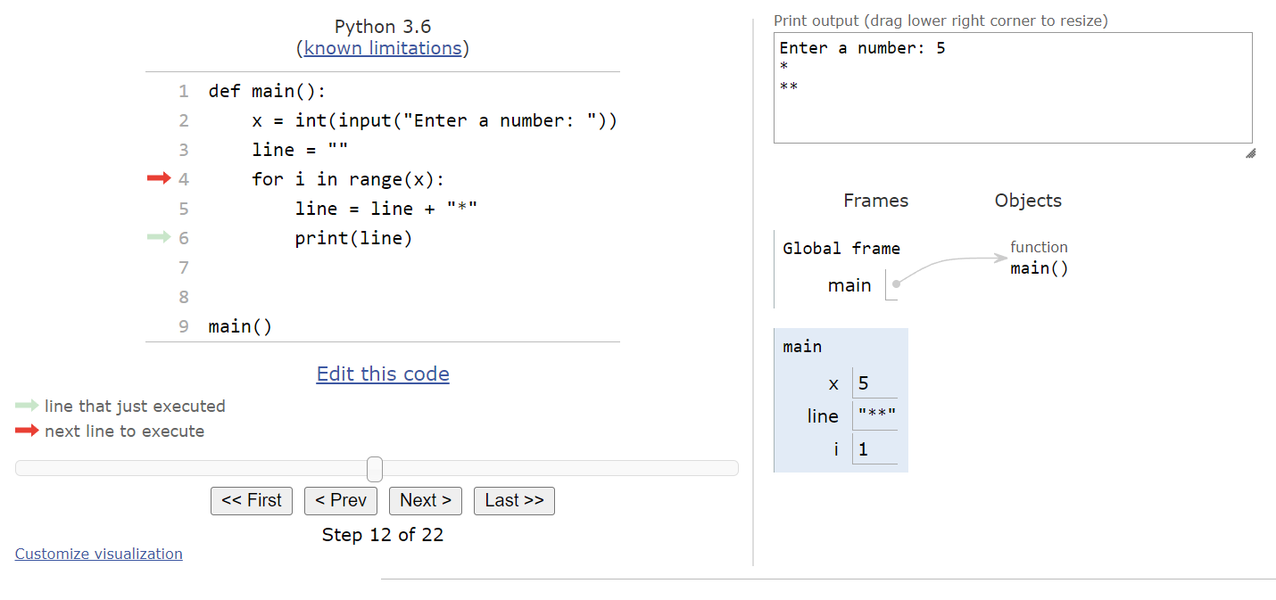
There are still more items in the list, so we’ll update i to the value $2$ and enter the loop:

In the loop, we’ll update line to contain one more asterisk, and then print it before looping back to the top.

The list still isn’t empty, so we’ll update i to be $3$ this time:

And then we’ll update line and print it.

By now, we should have a pretty good idea of what this loop does. There’s one more item in the list, so we’ll update i to be $4$:
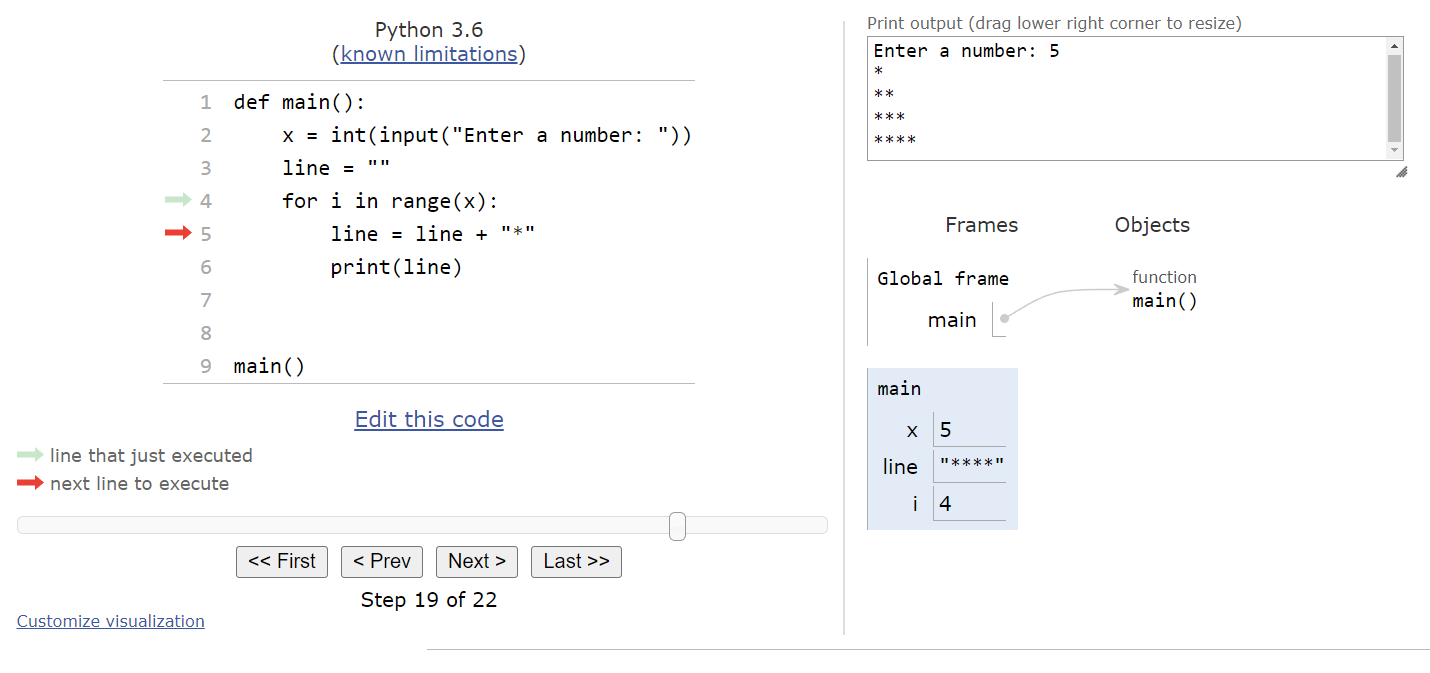
Inside the loop, we’ll add one more asterisk to line and then print it.
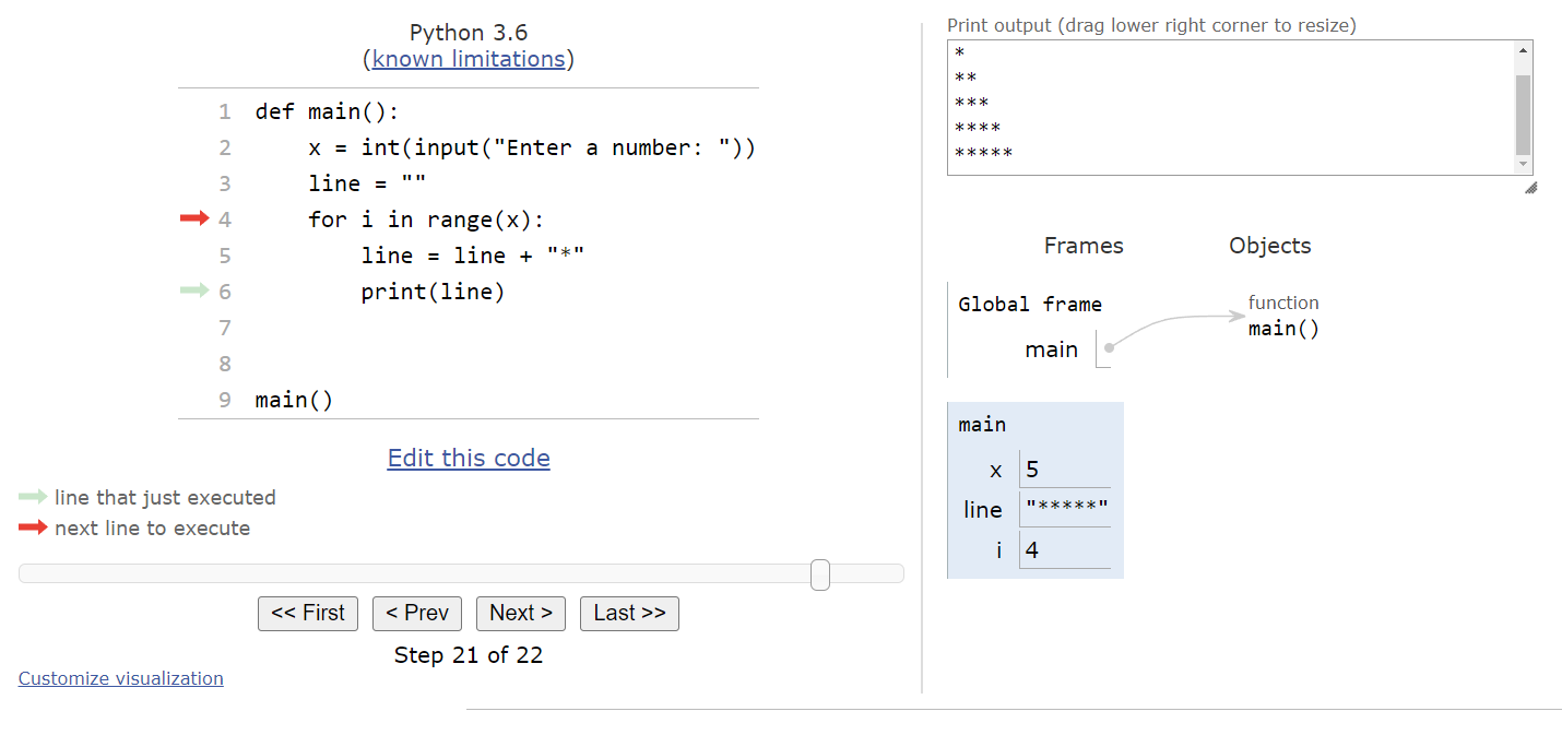
Finally, we’re back at the top of the loop. Since there are no more items left in the list, we can jump to the bottom of the for loop and continue the program from there. In this case, there’s no more code left in the main() function, so it will end and the program will terminate.
Looking at the output, we see that this program will print a right triangle of asterisks that is x lines tall and x characters wide at the bottom.
A full execution of this program is shown in this animation.
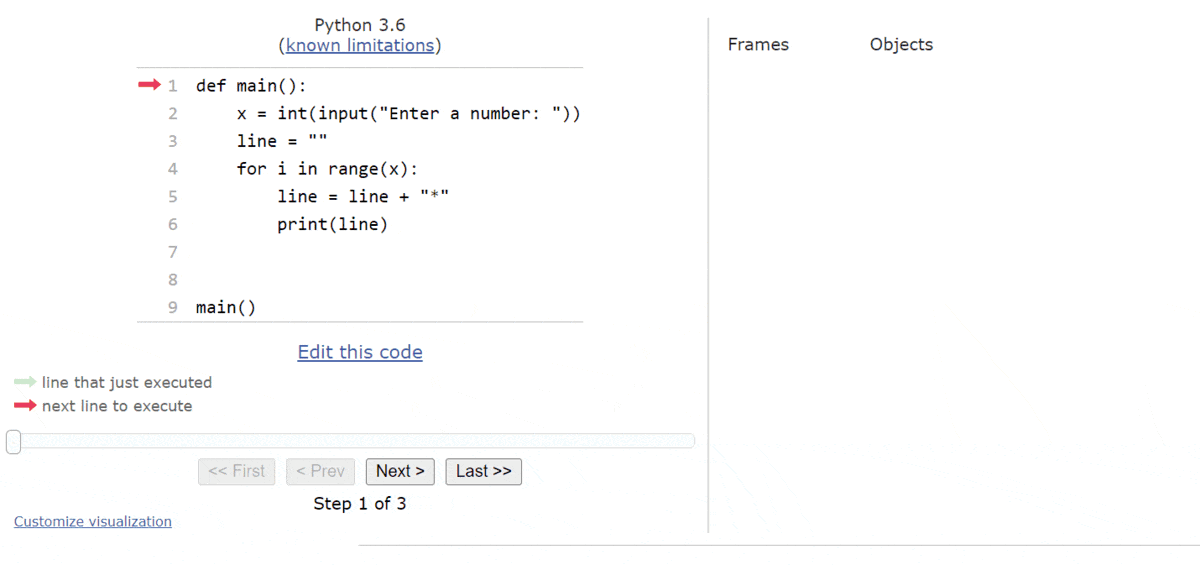
As we can see, working with for loops in Python is a quick and easy way to repeat a block of statements a specific number of times using the range() function.
It is possible to convert any for loop using the range() function in Python to a while loop. This can be done following a simple three-step pattern:
Let’s look at the main() function from the example above:
def main():
    x = int(input("Enter a number: "))
    line = ""
    for i in range(x):
        line = line + "*"
        print(line)
To convert this for loop into a while loop, we can follow the three steps listed above. First, we must set an initial value for our iterator variable i before the loop. Since the first value stored in i is $0$, we’ll set it to that value.
def main():
    x = int(input("Enter a number: "))
    line = ""
    i = 0
    for i in range(x):
        line = line + "*"
        print(line)
Next, we need to update the value of the iterator variable at the end of each loop iteration. Since we didn’t provide an argument for the step value in the range() function, we know that i will just be incremented by $1$ each time. So, we’ll add a short line to increment i at the bottom of the loop:
def main():
    x = int(input("Enter a number: "))
    line = ""
    i = 0
    for i in range(x):
        line = line + "*"
        print(line)
        i = i + 1
Finally, we can switch the for loop to a while loop. In the Boolean expression, we want to repeat the loop while the iterator variable i has not reached the maximum value. So, we’ll use the Boolean expression i < x in the new while loop:
def main():
    x = int(input("Enter a number: "))
    line = ""
    i = 0
    while i < x:
        line = line + "*"
        print(line)
        i = i + 1
There we go! That’s the basic process for converting any for loop using range() in Python to be a while loop. It’s a useful pattern to know and recognize when it is used in code.
Loops in Python are also a great way to handle situations where a user must input a value that meets certain criteria. Previously, we used an if statement to determine if the input was valid, but if it wasn’t valid all we could do was print an error and end the program. If we use a loop instead, we can prompt the user to provide additional input until we receive a valid value.
To make this process easy to use, we can develop a function just to handle input from the user. For example, if we want the user to input a percentage, we could use a function similar to this one:
def input_percentage():
    x = float(input("Enter a percentage as a decimal number from 0 to 1: "))
    while(x < 0 or x > 1):
        print("Invalid Input!")
        x = float(input("Enter a percentage as a decimal number from 0 to 1: "))
    return x
This function starts by prompting the user to input a number, and stores it as a floating-point value in the variable x. Then, it will reach the start of the while loop. The Boolean expression will check to see if the value provided is not a percentage, so if it is less than $0$ or greater than $1$ it is considered invalid.
If the input is invalid, we’ll print an error and prompt the user for input again. We’ll keep repeating this process until the user provides a value between $0$ and $1$, at which point the loop will terminate. The last line in the function will return that value back to where it was called from.
With a function such as that in our program, we can use it in another function such as the main() function to actually read input directly from the user. For example, we can write a quick program to calculate a weighted average of exam scores as shown below:
def input_percentage():
    x = float(input("Enter a percentage as a decimal number from 0 to 1: "))
    while(x < 0 or x > 1):
        print("Invalid Input!")
1.         x = float(input("Enter a percentage as a decimal number from 0 to 1: "))
    return x


def main():
    print("This program will compute weighted average for three exam scores")
    print("Enter the first exam's score")
    exam1_score = input_percentage()
    print("Enter the first exam's weight")
    exam1_weight = input_percentage()
    print("Enter the second exam's score")
    exam2_score = input_percentage()
    print("Enter the second exam's weight")
    exam2_weight = input_percentage()
    print("Enter the third exam's score")
    exam3_score = input_percentage()
    print("Enter the third exam's weight")
    exam3_weight = input_percentage()
    total = exam1_score * exam1_weight + exam2_score * exam2_weight + exam3_score * exam3_weight
    print("Your total score is {}".format(total))


main()
A quick execution of this program is shown here:
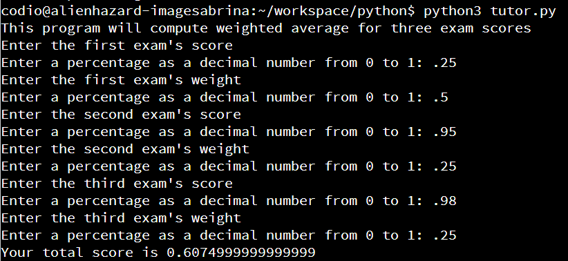
Take a minute to confirm that the program works by running it yourself, either in Python Tutor or directly in Python. You can even adapt this program to help calculate your final grade in this course!
Learning to how to create building blocks of larger programs, such as the input_percentage() function described here, is a great way to develop our programming skills. If we can learn to take a large program and break it down into smaller, repeatable chunks, then the entire program becomes much easier to develop and maintain.
Another important aspect of working with loops in code is learning how to properly test programs that contain loops. So, let’s look at some of the methods we can use when testing our programs containing loops to make sure they work correctly and won’t run into any problems.
Loops, like conditional statements, introduce different branches and paths into our programs. So, one of the first steps when testing these programs is to develop a set of inputs that will execute each branch of the code, as well as finding inputs that will execute multiple different paths through the program. Since loops may repeat many times, typically we only worry about two possible paths when dealing with loops - one path where it is skipped entirely and another path where the loop is entered at least once.
Let’s consider this simple Python program that contains loops:
def main():
    x = int(input("Enter a number: "))
    y = int(input("Enter a number: "))
    i = 0
    line = ""
    while i < x + y:
        line = line + "*"
        print(line)
        i = i + 1
    while i > x - y:
        print("=", end="")
        i = i - 1
    print()


main()
This program will simply print a right triangle of asterisks * that is x + y characters wide and tall, similar to a previous example in this lab. However, it will also print a final line of equals signs = below that, consisting of x - y characters. To test this program, we want to try and find some input values for x and y that achieve branch and path coverage.
To achieve branch coverage, we want to execute each line of code in this program at least once. An easy way to do that is to provide inputs so that the sum of x and y is a positive number in order to enter the first loop. After the first loop terminates, the value of i will be equal to the sum of x and y, provided that value is greater than $0$. So, in order to also enter the second loop, we need to make sure the difference of x and y is smaller than their sum.
A set of inputs that achieves this would be $3$ and $1$ for x and y, respectively. Their sum is $4$, so the first loop will be executed 4 times. Then, the difference between the values is $2$, so the second loop will executed twice to reduce the value in i to $2$.
So, we can say that the inputs 3 and 1 are enough to achieve branch coverage.
To achieve path coverage, we must consider three additional paths through the program:
First, in order to enter neither loop, we must have a set of inputs where the sum is less than or equal to $0$, and also where the difference is less than or equal to $0$. The simplest way to achieve this is to set both inputs to exactly $0$! Sometimes the simplest inputs are the easiest for testing.
To enter the first loop only, we need the situation where the sum of x and y is greater than 0, but then their difference is even larger. An easy way to accomplish this is to set y to a small negative number. For example, we could set x to $3$ and y to $-1$. That will make their sum $2$ but the difference $4$, so we’ll only execute the first loop but not the second one.
Finally, if we want to execute the second loop only, we need to make both the sum and the difference of x and y a number less than $0$. In that case, we can simply set both x and y to negative values, but make sure that x is overall a smaller value than y. So, we could set x to $-3$ and y to $-1$. In that case, their sum is $-4$ but their difference is $-2$. That will cause the program to skip the first loop but enter the second loop.
So, we can achieve path coverage with these four sets of inputs:
3, 10, 03, -1-3, -1When testing loops, we should also check to make sure that the loops will eventually terminate if we ever enter them. Thankfully, in this program, it is very easy to reason about this and convince ourselves that it works.
Consider the first loop - the only way to enter that loop is if the value of i is less than the sum of x and y, and each time the loop iterates the value in i will be incremented by $1$. Since i is getting larger each time, eventually it will reach a value that is greater than or equal to x + y and the loop will terminate.
The same argument can be made for the second loop. In that loop, i is initially greater than the difference of x and y, but i is decremented each time, so eventually the loop will terminate.
Technically speaking, we can come up with a loop variant for each loop and show that it is monotonically decreasing. This is easily done by simply finding the difference between the iterator variable i and the termination condition of the loop, either the sum or the difference of x and y. We won’t ask you to get to this level of detail when testing your own loops, but it is a very useful concept to understand when working with loops.
There we go! We were able to quickly come up with a set of inputs that will execute all possible branches and paths in this program, and we can also show that each of the loops will properly terminate anytime they are executed. So, we know that our program at least won’t crash, no matter what integers are provided as input. We can also examine the output of each test and make sure that it matches what the expected output should be in order to show that our program not only doesn’t crash, but that it provides the correct output.
Now that we’ve learned all about using loops in Python, let’s go through a complete worked example to see how all the pieces fit together. As we continue to develop larger and more complex programs, it is helpful to observe the entire process from start to finish so we can see how to easily develop a program one step at a time. Once we’ve created our program, we’ll also perform a bit of testing to make sure that it works correctly.
For this example, let’s write a program to play a simple number guessing game. Here’s how it works:
The game will select two random numbers from $0$ to $100$, one for each player. Then, each player will guess a number in the range, and the game will print either “higher” if that player’s secret number is larger than the guess, or “lower” if the player’s secret number is smaller than the guess. Players will alternate turns until one player correctly guesses their secret number and wins the game.
This game is pretty simple, but there are still quite a few different parts that we need to build in order to write the entire program. So, let’s go through the process of building a complete program in Python to play this game.
Before we start building our program, we need some way to generate a random number. Thankfully, Python has a built-in library called Random that has many functions for working with random numbers in our programs.
To use a library in Python, we must first import it into our code. This is done using a simple import statement at the very top of our program’s code, followed by the name of the library we want to use. So, for this library, we’ll need to have the following import statement at the top of our source code:
import randomOnce we’ve done that, we can use the function random.randint(a, b) to generate a random number that is between a and b, inclusive. Mathematically, we can say that it generates an integer $x$ such that $a <= x <= b$.
So, here’s a quick test program we can use to explore how to use random numbers in Python:
import random


def main():
    a = int(input("Enter a minimum value: "))
    b = int(input("Enter a maximum value: "))
    x = random.randint(a, b)
    print("A random number between {} and {} is {}".format(a, b, x))


main()
Take a minute to run this program and modify it a bit to make sure you understand how to work with random numbers in Python before continuing.
In Python, we know that all of our programs must include a main() function and a call to the main() function, so we can start building our solution by creating that basic structure as shown here:
def main()


main()
In the program itself, we need to start by generating two random numbers from $0$ to $100$, one for each player. So, we can create and store those numbers in the main() function, and we’ll also need to import the random library at the top of our file.
import random


def main():
    p1_secret = random.randint(0, 100)
    p2_secret = random.randint(0, 100)


main()
Once we have the secret numbers, then we can sketch out the game itself. We’ll use a while loop to repeat until a player has guessed correctly, and we’ll also use a simple integer variable to keep track of the current player. Inside of the loop, we should get a new guess from a player, and also switch between players. So, let’s add that to our program structure using some comments:
import random


def main():
    p1_secret = random.randint(0, 100)
    p2_secret = random.randint(0, 100)
    player = 1
    while( ): # player has not guessed correctly
        # swap player
        # get new guess from player
        # check if secret is higher or lower


main()
From here, we can start to work on the actual logic in our program.
The trickiest part of this program is coming up with the correct Boolean expression to use in our while loop. That helps us determine if the player has guessed correctly and that the loop should stop. However, this is a bit complex since there are two different players, each one with their own secret number. So, in our Boolean expressions, we have to determine what the current player is as well as whether the most recent guess was correct.
To do this, we can use the and and or Boolean operators to combine several Boolean expressions together. For example, we can determine if the current player is player 1 using player == 1, and then we can determine if the most recent guess is equal to player 1’s secret number using guess == p1_secret. If we want both of those to be True in order to exit the loop, we can combine them using the and operator. We can do something very similar for player 2 as well. Then, if we want the loop to terminate if either of those is true, we can combine the two statements using the or operator.
So, all together, we want to repeat the loop as long as that entire statement is not True. So, the full Boolean expression would be:
not ((player == 1 and guess == p1_secret) or (player == 2 and guess == p2_secret))That’s pretty complex, but it easily encompasses all of the rules of the game!
To get input from the user, we can write a simple read_input() function that is very similar to the ones we saw earlier in this lab. We simply want to make sure the user has provided a value that is between $0$ and $100$, and prompt the user for another input if not. We’ll also add in a parameter to print the current player in the prompt for input.
So, our read_input() function might look something like this:
def read_input(player):
    x = int(input("Enter a guess for player {}: ".format(player)))
    while x < 0 or x > 100:
        print("Invalid Input!")
        x = int(input("Enter a guess for player {}: ".format(player)))
    return x
Then, in our main() function, we can simply use the new read_input() function to read a player’s current guess as shown here:
def main():
    p1_secret = random.randint(0, 100)
    p2_secret = random.randint(0, 100)
    player = 1
    while(not ((player == 1 and guess == p1_secret) or (player == 2 and guess == p2_secret))): # player has not guessed correctly
        # swap player
        guess = read_input(player)
        # check if secret is higher or lower


main()Next, we need to add some conditional statements to check if the secret is higher or lower than the guess, and also to swap between players. First, let’s look at swapping players. This is pretty simple, since all we need to do is find out what the current player is, and switch that value to the other player. So, we can do that using a simple if statement as shown here:
def main():
    p1_secret = random.randint(0, 100)
    p2_secret = random.randint(0, 100)
    player = 1
    while(not ((player == 1 and guess == p1_secret) or (player == 2 and guess == p2_secret))): # player has not guessed correctly
        if player == 1:
            player = 2
        else:
            player = 1
        guess = read_input(player)
        # check if secret is higher or lower


main()
The process for checking a guess is very similar - we can simply check to see if the guess is higher or lower than the secret for the current player, and print the output accordingly. First, we’ll need to figure out the current player:
if player == 1:
    # check player 1's secret
else:
    # check player 2's secret
Then, in each of those branches, we’ll check the guess:
if player == 1:
    if guess < p1_secret:
        print("Higher")
    elif guess > p1_secret:
        print("Lower")
    else:
        print("Correct!")
else:
    if guess < p2_secret:
        print("Higher")
    elif guess > p2_secret:
        print("Lower")
    else:
        print("Correct!")
This is a pretty straightforward set of conditional statements, but it goes to show how many lines of code are required even for a simple guessing-game program like this one.
So, at this point, we can put all of the pieces together and test our program. Here is the complete program that we’ve written so far:
import random


def read_input(player):
    x = int(input("Enter a guess for player {}: ".format(player)))
    while x < 0 or x > 100:
        print("Invalid Input!")
        x = int(input("Enter a guess for player {}: ".format(player)))
    return x


def main():
    p1_secret = random.randint(0, 100)
    p2_secret = random.randint(0, 100)
    player = 1
    while(not ((player == 1 and guess == p1_secret) or (player == 2 and guess == p2_secret))):
        if player == 1:
            player = 2
        else:
            player = 1
        guess = read_input(player)
        if player == 1:
            if guess < p1_secret:
                print("Higher")
            elif guess > p1_secret:
                print("Lower")
            else:
                print("Correct!")
        else:
            if guess < p2_secret:
                print("Higher")
            elif guess > p2_secret:
                print("Lower")
            else:
                print("Correct!")


main()
So, let’s try to run this program and see if it works. Unfortunately, right from the start we have an error in our code, since when we try to execute this program, we’ll get the following error:
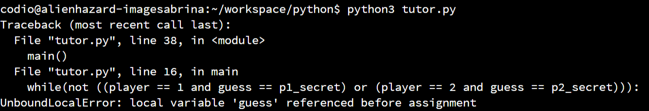
Take a minute to see if you can spot and fix the error before continuing!
Unfortunately, in our Boolean expression inside of the while loop, we’re referencing the guess variable, but that variable isn’t actually created until later inside the while loop itself. So, we’ll need to set the guess variable to a value outside of the while loop first.
Also, we must be very careful about what value we use. If we set guess to be $0$ initially, there is a very small chance that player 1 could win the game immediately if their secret number is $0$, since that is a valid guess. Instead, let’s set guess to be $-1$ so that it will never be equal to a secret number.
After we make that change, when we run the program again, we may notice one other error:
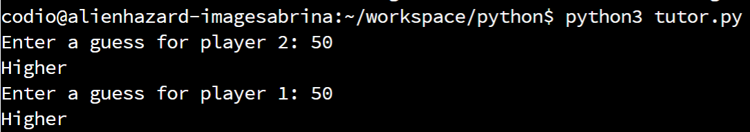
Can you spot it by looking at this screenshot?
Unfortunately, our program starts with player 2’s turn instead of player 1. Why is that? Well, if we look closely at our code, we see that we are initially setting the player to player 1, but then immediately switching players inside of the while loop before we prompt for input. If we think about it, we can’t move the code that swaps players to later in the while loop, because then our Boolean expression to determine if the while loop should terminate will be incorrect. So, instead, we can simply initialize the player variable to be $2$, and then it will be switched to $1$ before we prompt for input the first time.
So, our final working program’s code with these two changes is shown here:
import random


def read_input(player):
    x = int(input("Enter a guess for player {}: ".format(player)))
    while x < 0 or x > 100:
        print("Invalid Input!")
        x = int(input("Enter a guess for player {}: ".format(player)))
    return x


def main():
    p1_secret = random.randint(0, 100)
    p2_secret = random.randint(0, 100)
    player = 2
    guess = -1
    while(not ((player == 1 and guess == p1_secret) or (player == 2 and guess == p2_secret))):
        if player == 1:
            player = 2
        else:
            player = 1
        guess = read_input(player)
        if player == 1:
            if guess < p1_secret:
                print("Higher")
            elif guess > p1_secret:
                print("Lower")
            else:
                print("Correct!")
        else:
            if guess < p2_secret:
                print("Higher")
            elif guess > p2_secret:
                print("Lower")
            else:
                print("Correct!")


main()
A full example of running this program, complete with a very lucky guess, is shown in the screenshot below:
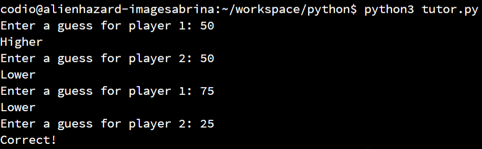
Now that we have a complete and working program, let’s look at what it might take to test it. Unfortunately, testing a program that uses random numbers can be very tricky, since each time you run the program you might receive different outputs even if you provide the same inputs.
Thankfully, we can still perform some testing to achieve branch and path coverage by choosing our guesses carefully. Here are the basic methods we’ll want to try:
"Higher" for output, unless the secret number is $0$."Lower" for output, unless the secret number is $100$."Correct". Using a bit of logic, it is always possible to win the game in no more than $7$ guesses."Invalid Input!" for output at least once.Following those simple strategies and keeping track of the various outputs received, it is pretty easy to eventually test all branches and most, if not all, possible paths through the program.
Checking for loop termination on this program is a bit trickier, since the secret numbers are random and the guesses that a player makes are also unpredictable. So, while we can’t say for sure that the program will terminate, we can always prove that there is a possible condition where the loop will terminate, and that condition depends entirely on the user providing the correct input. So, as long as it is possible, we can say that the loop is at least not an infinite loop, and the program will work correctly if the user makes the correct guess.
There we go! We’ve just explored a complete example of writing a program in Python, complete with loops and conditional statements. We also introduced random numbers and how we can easily use those in our programs. Beyond that, we explored how to test these programs and correct minor errors found in testing. Hopefully this process is very helpful as we continue to work on larger and more complex programs.
In this lab, we introduced several major important topics in Python. Let’s quickly review them.
While loops in Python will execute while a Boolean expression evaluates to true.
while <boolean expression>:
<block of statements>The range() function in Python is used to generate a list of numbers. It can be used in three ways:
range(stop) - numbers from $0$ up to (but not including) stoprange(start, stop) - numbers from start up to (but not including) stoprange(start, stop, step) - numbers from start up to (but not including) stop, with step between each number.For loops in Python will execute a set number of times.
for <iterator variable> in <list>:
<block of statements>Loops can be used to request new input from the user if invalid input is received.
def input_percentage():
    x = float(input("Enter a percentage as a decimal number from 0 to 1: "))
    while(x < 0 or x > 1):
        print("Invalid Input!")
        x = float(input("Enter a percentage as a decimal number from 0 to 1: "))
return xLoops can be tested for both branch and path coverage. In general, achieving path coverage involves writing code that will enter the loop, and also code that will bypass the loop entirely.
Loops should also be tested for termination and situations that may result in infinite loops. Using a loop variant and showing that it is monotonically decreasing is a helpful technique.
To create a nested loop in Python, we can simply place a loop structure inside of the block of statements that is repeated by another loop structure. This is very similar to how we can nest conditional statements as well.
For example, consider this short Python program:
def main():
    i = 1
    while i < 10:
        j = i
        while j < 10:
            print("{} ".format(j), end="")
            j = j + 1
        print("")
        i = i + 1
    print("Complete!")


main()
In this example, we see a Python while loop that uses the variable i in its Boolean expression first, and then inside of that loop we see another loop that uses j in its Boolean expression. When we run this code, each time we execute the steps inside of the outer while loop, we’ll have to completely go through the inner while loop as well. It can be very complex to keep track of everything, but with a bit of practice we’ll learn some strategies for mentally working through loops.
Before continuing, take a look at that program’s code and see if you can determine what it will print!
To really understand how a set of nested loops work, let’s go through a code tracing example using Python Tutor. To follow along, place this code in the tutor.py file in the python folder on Codio, or click this Python Tutor
link to load Python Tutor in a web browser.
When we first load this code in Python Tutor, we should see the following state:
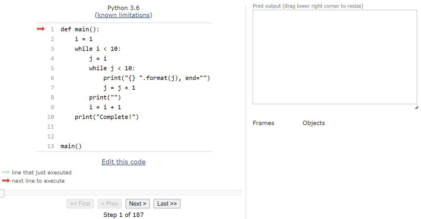
When we look at the bottom of the Python Tutor page, we’ll see that we are on step 1 of 187 steps! That’s a very large number of steps to deal with! Up to this point, most of our programs have been around 20 or 30 steps in total. So, already we’re seeing that nested loops can quickly create programs that execute many more steps.
If we click next a few times, we’ll see Python Tutor find the main() function definition, and then call that function from the bottom of the code. By the time we’ve entered the main() function, we should be at this state:
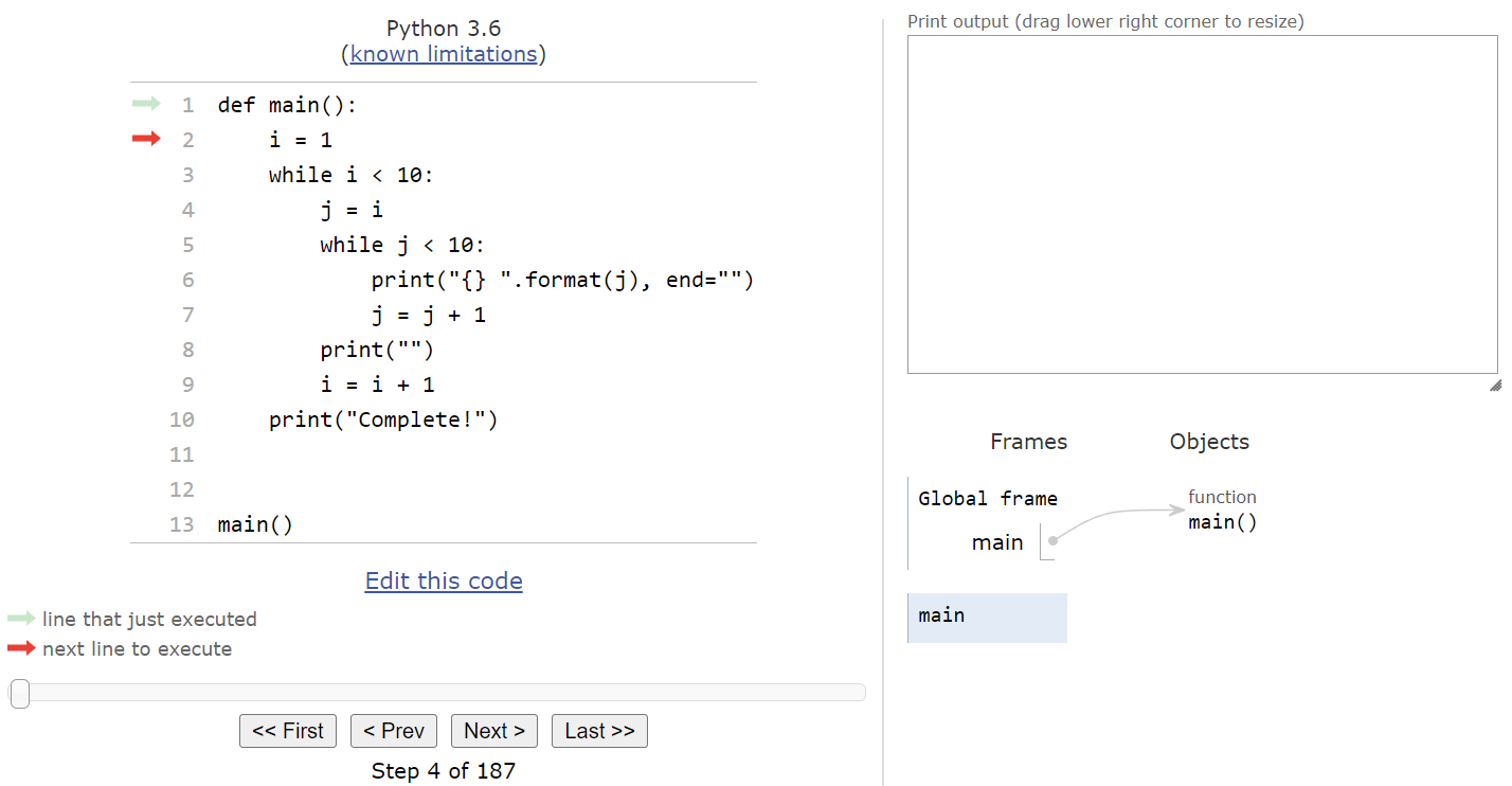
Here, we are setting up the iterator variable i that is used for the outermost loop. So, we’ll store the value $1$ in i and then move to the next line:
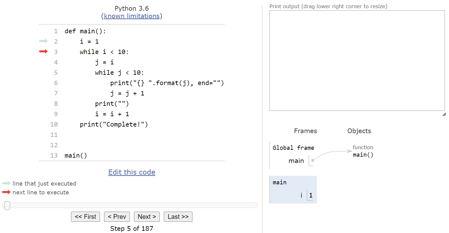
Now we’re at the start of our outer while loop. That means that we’ll need to evaluate the Boolean expression and determine if it is True or False. In this case, we can see that i < 10 will evaluate to True, so we should enter the loop.
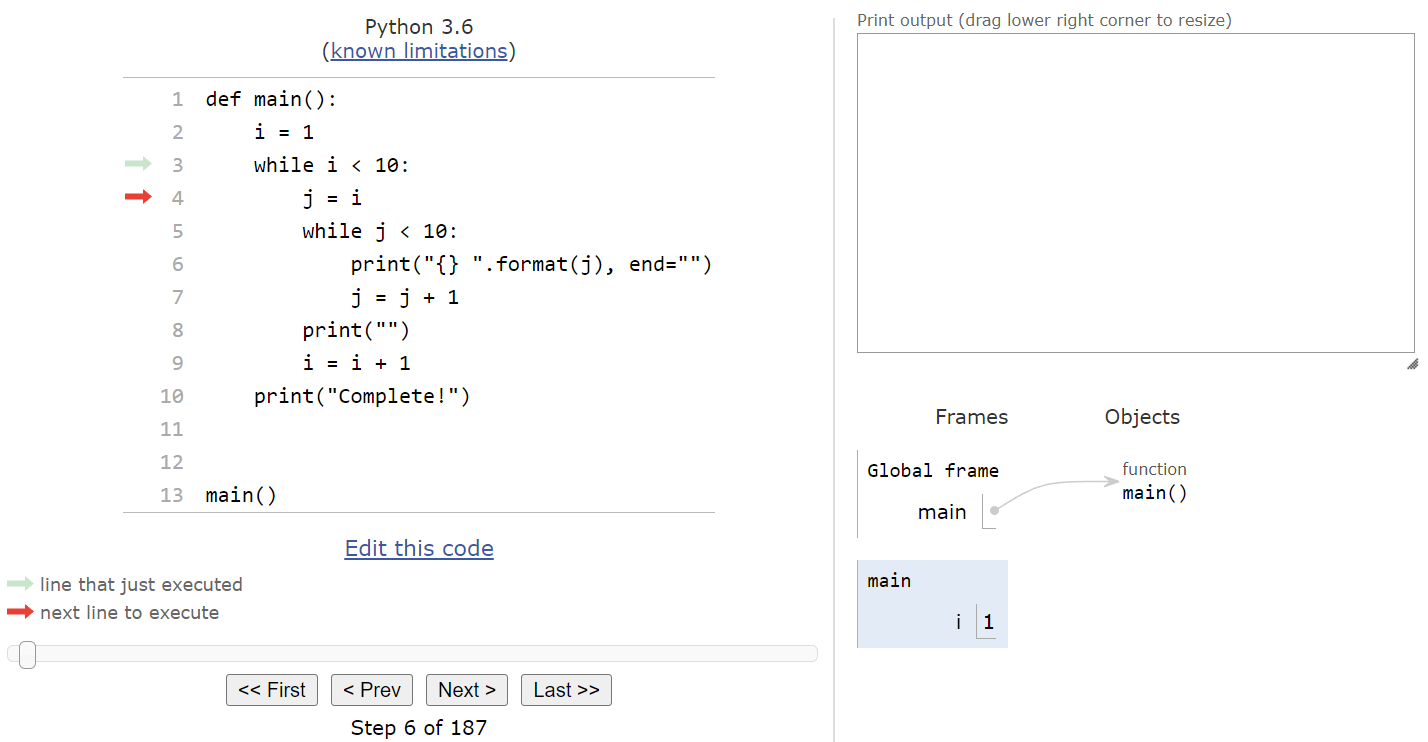
Once we are inside the loop, we’ll start setting up the iterator variable j for the inner loop. In this code, we are storing the current value of i in j, so at this point j will also contain $1$.

At this point, we need to decide if we should enter the inner while loop. So, once again we’ll look at the Boolean expression, j < 10, and see that it is also True and we should enter the loop.

Inside of the inner while loop, we’ll perform two actions. First, we’ll print the current value of j to the output, but we won’t move to the next line since the end parameter is set to an empty string in the print() function:
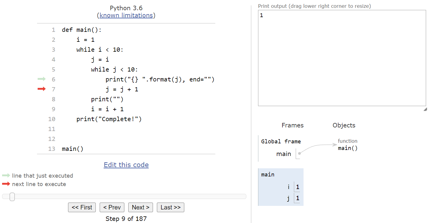
Then, we’ll increment the value of j by $1$ before looping back to the top of the innermost loop:

Notice that when we reach the end of the innermost loop, we jump back to the beginning of that loop, NOT to the beginning of the outermost loop. This is an important concept to learn - since we are only dealing with the inner loop at this point, we must continue to repeat its steps until the Boolean expression evaluates to False. So, since the Boolean expression j < 10 still evaluates to True, we should enter the loop once again.

Inside the loop, we’ll print the current value of j to the same line of output as before:

And once again we’ll increment the value of j by $1$ and jump back to the top of the innermost while loop:
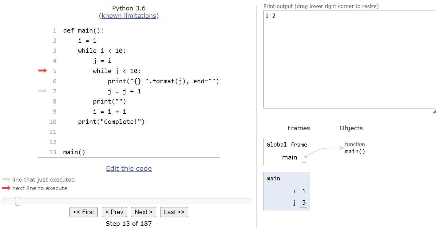
Hopefully at this point we have a pretty good idea of what each step of the innermost while loop does. It will simply print the value of j and increment it by $1$, repeating those steps until j is greater than or equal to $10$. So, once the inner while loop terminates, we’ll see this state:

We jumped from step 13 to step 35 just to complete the inner while loop. Finally, at this point we’ll print an empty string, which will move our output to the next line, and then we’ll increment the value in i by $1$ before looping to the top of the outer while loop:
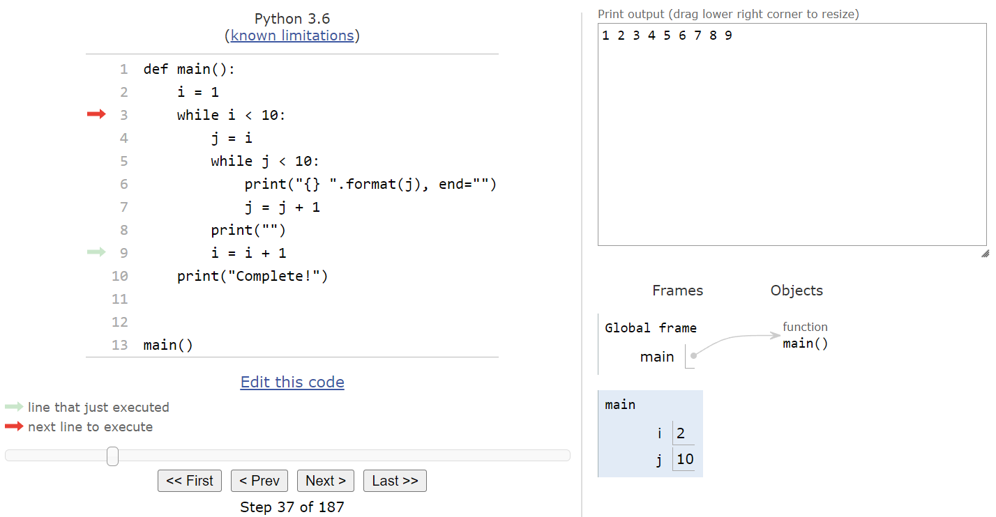
Now we must check to see if we should enter the outer while loop again by checking the Boolean expression i < 10. Since that evaluates to True, we’ll enter the loop a second time.

Inside the loop, we’ll reset the value of j to be the current value stored in i, which is now $2$, and then we’ll reach the inner while loop:
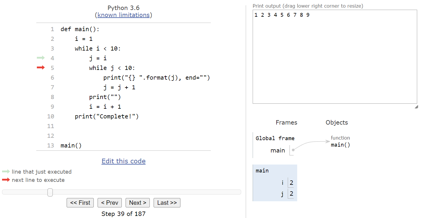
Here, we can evaluate the Boolean expression j < 10, which is currently True, and determine that we should enter the inner while loop.

Inside the loop, the code hasn’t changed, so we can use our understanding from before to quickly figure out what this loop does. It will print the current value in j and then increment j by $1$, so we’ll end up at this state:

At this point, we can easily assume that the inner loop will do pretty much the same thing as before - it will print all of the values from i up through $9$ to the output, all on the same line. So, once the inner loop has completely finished, we’ll see the following state in Python Tutor:

We were able to quickly jump from step 42 all the way to step 64 just by understanding what the inner loop is doing and extrapolating from our previous experience. Now, we can finish up this iteration of the outer loop by printing a newline and then incrementing i by $1$, and then we’ll be back at the beginning of the outer while loop:

At this point, we’ve completely worked through two iterations of the outermost while loop, including two complete executions of the innermost while loop. So, we’re at a good point to make a prediction about the output of the program as a whole, without executing the next 120 steps. It looks like the inner loop will print the values from i through $9$ on a single line, and then each line will start with the value of i being incremented by $1$ each time. So, overall, we can expect the entire outer while loop to produce the following output:
1 2 3 4 5 6 7 8 9
2 3 4 5 6 7 8 9
3 4 5 6 7 8 9
4 5 6 7 8 9
5 6 7 8 9
6 7 8 9
7 8 9
8 9
9
And, indeed, if we jump ahead to the last line of the program we’ll see exactly that situation in Python Tutor:
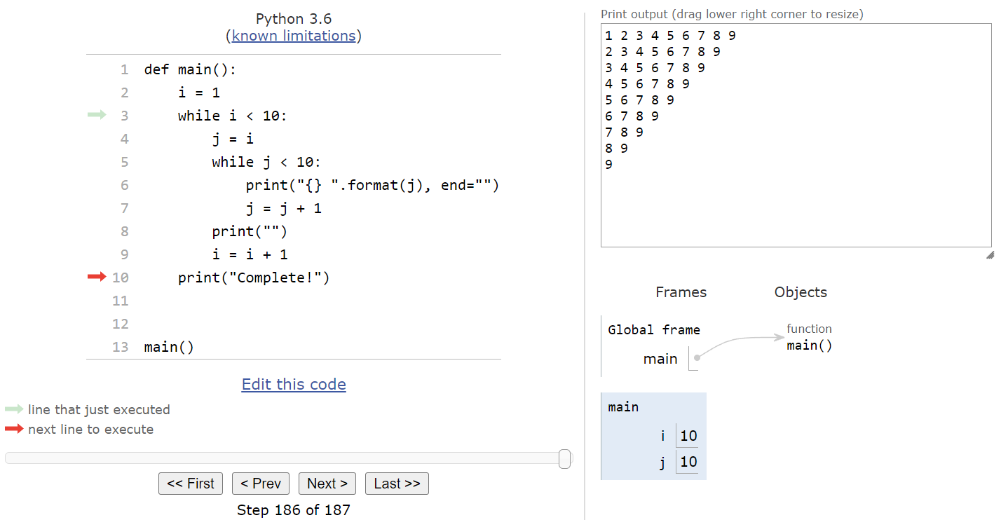
The program ends by printing the string "Complete!". At the end of the program, we’ll see the following state:
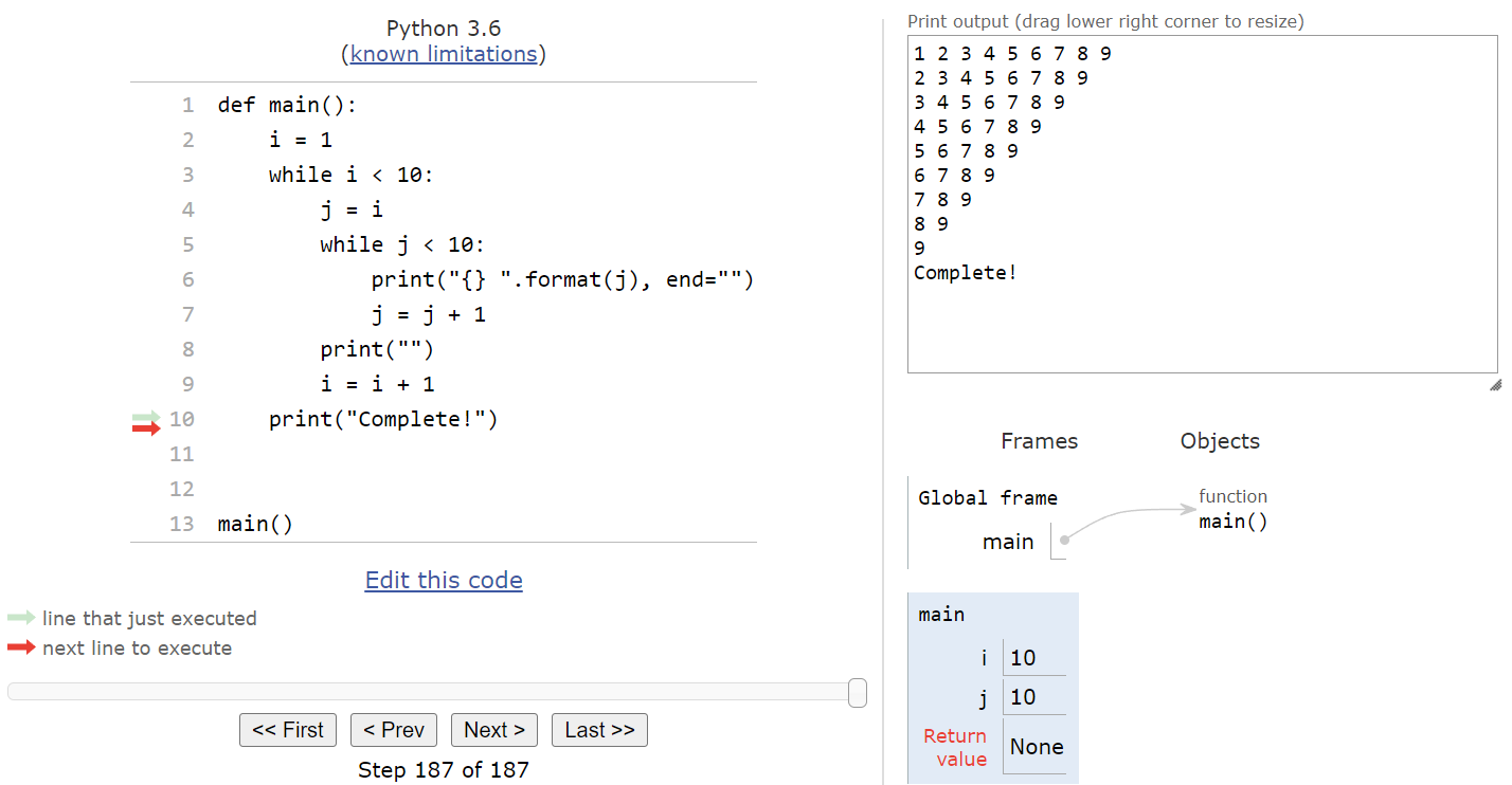
A full animation of this process is shown here. After the first full iteration of the outer while loop, the rest of the internal steps are omitted and only the end of each loop iteration is shown.
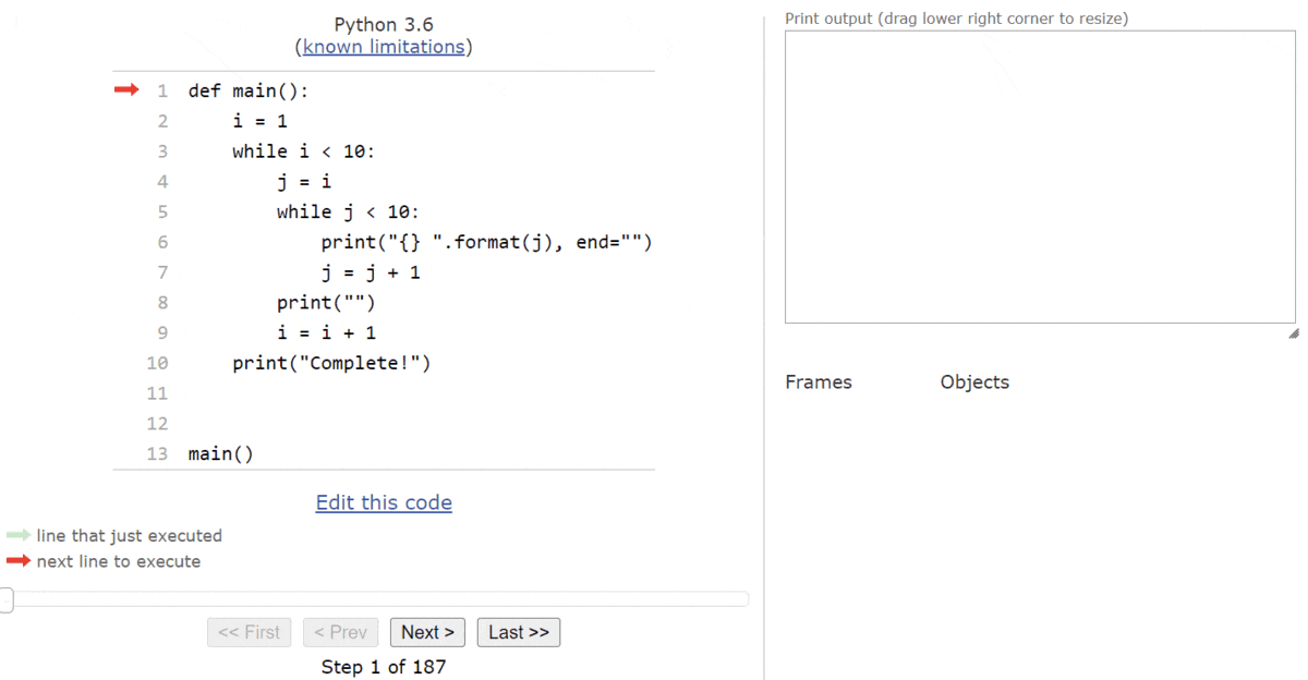
Working through an example program such as this one is a great way to explore how nested loops work in Python
Writing code that has nested while loops can be quite tricky, as there are several pitfalls that we might encounter. Here are a few tips to keep in mind when designing code that uses nested while loops:
Nested loops present a very difficult challenge for programmers, because they are short snippets of code that may end up resulting in hundreds or even thousands of individual steps to be executed. So, anything we can do to make the loops simpler and easier to understand will greatly improve our ability to write programs with fewer bugs.
For loops can also be nested, just like while loops. In fact, nesting for loops is often much simpler than nesting while loops, since it is very easy to predict exactly how many times a for loop will iterate, and also because it is generally easier to determine if a for loop will properly terminate instead of a while loop.
A great way to explore using nested for loops is by printing ASCII Art shapes. For example, consider the following Python program that contains nested for loops:
def main():
    for i in range(3):
        for j in range(5):
            print("* ", end="")
        print("")


main()
Just by looking at the code, can you predict what shape it will print? We can check the result by running the program on the terminal directly. If we do so, we should receive this output:
* * * * *
* * * * *
* * * * *
It printed a rectangle that is $3$ rows tall (the outer for loop) and $5$ columns wide (the inner for loop). If we look back at our code, this hopefully becomes very clear. This is a very typical structure for nested for loops - the innermost loop will handle printing one line of data, and then the outer for loop is used to determine the number of lines that will be printed.
The process for dealing with nested for loops is nearly identical to nested while loops. So, we won’t go through a full example using Python Tutor. However, feel free to run any of the examples in this lab in Python Tutor yourself and make sure you clearly understand how it works and can easily predict the output based on a few changes.
Let’s look at a few more examples of nested for loops and see if we can predict the shape that is created when we run the code.
def main():
    for i in range(5):
        for j in range(i + 1):
            print("* ", end="")
        print("")


main()
This time, we’ve updated the inner for loop to use range(i + 1), so each time that inner loop is reached, the range will be different based on the current value of i from the outer loop. So, we can assume that each line of text will be a different size. See if you can figure out what shape this will print!
When we run the code, we’ll get this output:
*
* *
* * *
* * * *
* * * * * We see a triangle that is $5$ lines tall and $5$ columns wide. If we look at the code, we know that we’ll have 5 rows of output based on the range(5) used in the outer loop. Then, in the inner loop, we can see that the first time through we’ll only have a single item, since i is $0$ and the range used is range(i + 1).
The next iteration of the outer loop will have $1$ stored in i, so we’ll end up repeating the inner loop $2$, or i + 1, times. We’ll repeat that process until the final line, which will have $5$ characters in it to complete the triangle.
From here, we can quickly modify the program to change the structure of the triangle. For example, to flip the triangle and make it point downward, we can change the range in the inner loop to range(i, 5) instead!
What if we want to flip the triangle along the vertical axis, so that the long side runs from the top-right to the bottom-left? How can we change our nested loops to achieve that outcome?
In that case, we’ll not only have to print the correct number of asterisks, but we’ll also need to print the correct number of spaces on each line, before the asterisks. One possible way to achieve this is shown in this code:
def main():
for i in range(5):
for j in range(4 - i):
print(" ", end="")
for j in range(i + 1):
print("* ", end="")
print("")
main()Here, we have two for loops nested inside of our outer loop. The first loop creates a range using the expression 4 - i, and the second loop uses the expression i + i. So, when i is equal to $0$ during the first iteration of the outer loop, the first inner loop will be executed $4$ times, and the second loop only $1$ time. Then, on the next iteration of the outer loop, the first inner loop will only run $3$ times, while the second loop now runs $2$ times. Each time, the sum of the iterations will be $5$, so our lines will always be the same length.
When we run the code, we’ll get this output:
*
* *
* * *
* * * *
* * * * * Up to this point, we’ve just been writing loops to print shapes using ASCII art. While that may seem trivial, understanding the “shape” that will be produced by a given set of nested loops can really help us understand how the code itself will function with other data.
Consider this example code:
def main():
sum = 0
count = 0
for i in range(10):
for j in range(i + 1):
sum = sum + (i * j)
count += 1
print("sum: {}, count: {}".format(sum, count))
main()Before we even try to run this code, can we guess what the final value of the count variable will be? Put another way, can we determine how many times we’ll execute the code in the innermost loop, which will help us understand how long it will take for this program to run?
Let’s compare this code to the first example shown above:
def main():
for i in range(5):
for j in range(i + 1):
print("* ", end="")
print("")
main()Notice how the code structure is very similar? The outermost loop runs a given number of times, and then the inner loop’s iterations are determined by the value of the outer loop’s iterator variable. Since we know that the first example produces a triangle, we can guess that the program above runs in a similar way. So, the first iteration of the outer loop will run the inner loop once, then twice on the second iteration, and so on, all the way up to $10$ iterations. If we sum up all the numbers from $1$ to $10$, we get $55$.
Now let’s run that code and see if we are correct:

As this example shows, we can use our basic understanding of various looping structures to help us understand more complex programs, and even predict their output without running or tracing the program. This is a very useful skill to learn when working with nested loops.
Testing nested loops can also be very tricky, especially because they can make our program’s control flow even more complex. So, let’s briefly go through an example to see how to determine what inputs we can use to test nested loops.
Consider the following example program:
def positive_input():
x = int(input("Enter a positive integer: "))
while x <= 0:
print("Invalid input!")
x = int(input("Enter a positive integer: "))
return x
def main():
x = positive_input()
y = positive_input()
while y <= x:
for i in range(x - y):
print("*", end="")
y = y + 2
print("")
print("Complete!")
main()Let’s work through the process of generating some test cases for this program to see if it runs without any errors. As always, our biggest concern is to make sure that we don’t reach a situation where the program enters an infinite loop, and that we also try to provide inputs that will enter each loop at least once, and also bypass each loop if possible.
First, we see that the positive_input() function uses a loop to make sure the user inputs only positive values. So, some of our first test cases could involve trying values such as $-1$, $0$ and $1$ to check the edge cases of that while loop’s Boolean expression. When we run the program and provide those inputs, we should see it enter the loop in that function at least once.
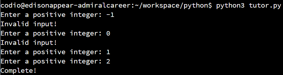
We can also bypass that loop by simply making sure we enter a positive integer each time. So, we know we have a few test cases available that will achieve branch coverage for that loop.
Next, let’s consider the outermost while loop in the main() function. That loop uses the Boolean expression y <= x to determine if the loop should be entered or not. So, we want to come up with a few tests that check the edge cases of that Boolean expression. We can start by choosing a value to use for x, such as $5$. Then, the edge cases of that Boolean expression would be when y is either $4$, $5$, or $6$.
If y is $6$, the Boolean expression would be False and it should bypass the loop. We can easily test this to make sure that is the case:
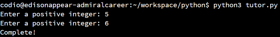
Likewise, if y is $4$, we know that it should enter the outermost loop. Inside, we see a for loop that will iterate based on the expression x - y. Effectively, it will compute the difference between x and y and then iterate that many times. So, if x is $4$ and y is $5$, the difference between those values will be $1$. So, we’ll enter the innermost for loop at least once. When we run the program with these inputs, we’ll see the following output:
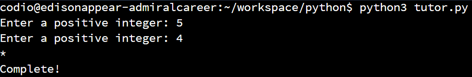
What if we set both x and y to be the same value? We know that the inner for loop will run x - y times, so if both x and y are the same value, this would be a way to bypass that loop, while still entering the outermost while loop since y <= x will be True. However, when we try to run the program with these inputs, we’ll see something interesting happen:
Our program will quickly start printing blank lines of output to the terminal. So quickly, in fact, that it is hard to even see what happens. As it turns out, we accidentally caused our program to enter an infinite loop! When this happens, the only way to stop the program is to close the terminal window it is running in, or use the CTRL+C keyboard command to interrupt it. So, let’s see why this infinite loop is occurring, and figure out how we can fix it.
Did you spot the infinite loop when you first read the program’s code? It can be really tricky to find, which is why we have to be very good about choosing test cases that will explore many different ways to run the program.
In this case, the infinite loop is caused by the interaction between the two loops. In the outermost while loop, we have the Boolean expression y <= x to enter the loop. However, inside that loop, the for loop will only execute x - y times, which also happens to be the loop variant for the outer while loop. The key to the infinite loop lies in the fact that the only line inside of the outer while loop that will change the value of either x or y is also inside of the inner for loop. So, if we don’t execute the for loop’s code at all, then the value of x and y won’t change either, and we’ll continually repeat the steps of the outermost while loop.
There are many ways to fix this problem, but the simplest would be to change the Boolean expression of the outermost while loop to be y < x. That will ensure that there is at least one iteration of the innermost for loop, and the infinite loop condition will be avoided.
So, as this example shows, testing nested loops is just like testing regular loops - we want to try and find inputs that will enter the loop at least once, as well as inputs that will bypass the loops if possible, just to make sure there aren’t any strange situations that may arise. While this won’t find all errors that are present in code containing nested loops, it is a great way to start testing your programs.
Now that we’ve explored how to create programs that contain nested loops, let’s work through a complete example problem to see how we can convert a problem statement into working code.
Consider the following problem statement:
Write a program to print the sum of the first
nprime numbers, wherenis provided as input from the user.
This is a very simple problem statement, but it can be very complex to build a program that satisfies it. So, let’s go through the steps and see if we can get it to work.
As always, we can start building our programs by adding a main() function and a call to the main() function to our code, as shown here:
def main():
main()Inside of the main() function, the first thing we’ll need to do is get input from the user, since we really can’t do anything else until we know what our goal is. While the problem statement doesn’t include any information about what inputs are acceptable, we can infer that only positive integers should be used as input. So, we can borrow the positive_input() function from earlier in this module to handle all of our input:
def positive_input():
x = int(input("Enter a positive integer: "))
while x <= 0:
print("Invalid input!")
x = int(input("Enter a positive integer: "))
return x
def main():
n = positive_input()
main()Reusing existing code, such as the positive_input() function we just included here, is a great way to build our programs. We can always think of previous code that we’ve already written and tested as possible building blocks for future programs, and reusing existing code is a great way to speed up our development process.
Next, we need some way to determine if a number is a prime number. Recall from mathematics that a prime number is a number that is only equally divisible by $1$ and itself. For example, $7$ is prime, but $8$ is not since it can be evenly divided by $4$.
Thankfully, we know that we can use the modulo operator % to determine if a number if evenly divisible by another number. So, all we need to do is check if each number less than our chosen number can equally divide it. If none of them can, then our chosen number is prime.
So, let’s write a function that performs this operation. We’ll start by creating a function that accepts our chosen number as a parameter:
def is_prime(n):Next, we know that we need to check all of the numbers from $2$ up to but not including n. We can do this using a for loop and the range() function:
def is_prime(n):
for i in range(2, n):Inside of the for loop, we want to check and see if the iterator variable i can evenly divide the chosen number n using the modulo operator:
def is_prime(n):
for i in range(2, n):
if n % i == 0:
# i equally divides nHere’s where things get a bit tricky - if i can equally divide n, we know that n is not prime and we don’t have to check any other values. So, in our function, we can just use the return False statement to return the value False from this function. As soon as the function reaches a return statement, even if it is inside of a loop, it will immediately stop the function and go back to where it was called from. In effect, we can use this to shortcut the rest of the loop.
def is_prime(n):
for i in range(2, n):
if n % i == 0:
return False
# what if we don't return false?However, what happens if we check all of the values from $2$ up to n and don’t find a single one that will equally divide our chosen number n? In that case, we’ll reach the end of our for loop, but our function hasn’t returned anything. So, we’ll need to add one extra line to the end of the function to return True if we get to that point.
def is_prime(n):
for i in range(2, n):
if n % i == 0:
return False
return TrueThere we go! That’s a quick and easy function to determine if a given number is prime. This function is a great example of a pattern that we’ll see many times as we write complex programs whenever we must determine if a particular situation is true for a given list of numbers. Inside of the loop, we’ll check each case and return False if it isn’t true. If it is true, then we’ll complete the entire loop without returning False, so we’ll need to return True at the end of the function. We’ll see this pattern again in a later lab.
The is_prime() function above is very simple, but not very efficient. With a bit of thought, it is easy to determine that we only have to actually check numbers up to n /2, since it is impossible for any number larger than that to evenly divide n. Likewise, we can do some quick math to eliminate numbers that end in an even digit or $5$, since those numbers will never be prime.
Finally, we could use a more advanced mathematical technique such as the Sieve of Eratosthenes to generate all prime numbers more quickly. However, for this example, we’ll stick to the simplest approach.
Finally, now that we have the is_prime() function, we can complete our main() function by simply iterating through all possible numbers until we’ve found n prime numbers, and then print the sum:
def main():
n = positive_input()
count = 0
i = 2
sum = 0
while count < n:
if is_prime(i):
sum = sum + i
count = count + 1
i = i + 1
print("The sum of the first {} prime numbers is {}".format(n, sum))This program requires three additional variables. The variable count is used to keep track of the number of prime numbers found, so we’ll increment it inside of the if statement each time we find a prime number. Likewise, the sum variable keeps track of the sum of the prime numbers, which we’ll print at the end. Finally, we use i as our iterator variable, so we must make sure that we increment i each time the while loop iterates, outside of the if statement. We’ll start i at $2$, since $1$ is not a prime number mathematically. A very common programming mistake is to forget to increment i outside the if statement, resulting in an infinite loop. Also, we chose to use a while loop instead of a for loop since our program’s goal is to sum up the first n prime numbers, which is better expressed as a while loop instead of a for loop.
The full program is shown below:
def positive_input():
x = int(input("Enter a positive integer: "))
while x <= 0:
print("Invalid input!")
x = int(input("Enter a positive integer: "))
return x
def is_prime(n):
for i in range(2, n):
if n % i == 0:
return False
return True
def main():
n = positive_input()
count = 0
i = 2
sum = 0
while count < n:
if is_prime(i):
sum = sum + i
count = count + 1
i = i + 1
print("The sum of the first {} prime numbers is {}".format(n, sum))
main()Finally, notice that this program doesn’t contain a loop nested within another loop in the same function, but because we are calling the is_prime() function, which contains a loop, from within a loop inside of the main() function, it actually has a nested loop structure inside of it! Feel free to run this program in Python or using Python Tutor to confirm that it works as expected before continuing.
Testing this program is a bit complex, since we can only provide a single input. We can easily provide a negative value or $0$ to confirm that the loop in the positive_input() function is working correctly, but beyond that we have little control over the rest of the program just by changing inputs.
Instead, we have to rely on our ability to read and analyze the code to determine if it is working properly. For example, we can look at the loop inside of the main() function. It is a while loop, which relies on the count variable increasing until it is greater than or equal to n before it will terminate. We can see that count will be incremented each time the is_prime() function returns True, so as long as we are able to find enough prime numbers, and assuming our is_prime() function works correctly, this loop should eventually terminate.
In the is_prime() function, we have a simple for loop, which will always terminate eventually. There is no way to bypass it, so we don’t really have to worry about that function not eventually returning a value.
However, proving that this program creates the correct answer is a bit trickier. One of the best ways to do this is to simply check a few answers manually. For example, with a bit of searching online, we can find a list of prime numbers. According to Wikipedia , the first 9 prime numbers are:
2
3
5
7
11
13
17
19
23The sum of those numbers is easy to calculate using a calculator or other device, and eventually we can be fairly certain that the correct answer is $100$. When we run our program, we should hopefully get the same result:

We can test a few other numbers until we are sure that our program is working correctly.
Hopefully this example is a good look at how to build a program using loops that meets a given problem description. We were able to put together various types of loops and conditional statements in our program, and then test it to be sure it works. As you continue to work on projects in this class, feel free to refer back to these examples for ideas and blocks of code that you may want to use in your own programs. Good luck!
In this lab, we introduced several major important topics in Python. Let’s quickly review them.
Loops in Python can be nested, just like any other statement. While loops and for loops can be nested in any combination.
When testing nested loops, it is important to consider situations where a loop will be executed and where it will be bypassed. It is also important to consider the loop variants for while loops to ensure that there aren’t situations where a loop will accidentally run infinitely.
Nested loops can result in programs that execute many individual steps, even using just a few lines of code. It is always helpful to think about the number of times a loop will execute and make sure that it isn’t executing more times than necessary.
The first collection we’ll review in Python is the list. A list in Python allows us to store many individual values, or elements, in a single variable. To keep track of the elements, each one is assigned an index, which is an integer that uniquely identifies the element’s position in the list. In Python, just like in many other programming languages, the indexes begin at $0$ and count up from there.
There are many ways to create a list in Python. The simplest is to simply use an empty set of square brackets [] to represent an empty list, and then store that in a variable using an assignment statement:
list_1 = []If we know what values we want to store in the list, we can include them inside of the square brackets. For multiple items, we can separate them by commas:
list_2 = [1, 2, 3]We can store any value in a list, including strings, numbers, Boolean values, and even other lists. We won’t cover lists inside of lists in this course, but it is important to know that it can be done.
Once we’ve created a list, there are two ways to add items to a list. First, if we want to add a new item to the list and expand it’s size by one, we can use the append() method. For example, we can start with a list containing three items and then add a fourth item:
list_2 = [1, 2, 3]
list_2.append(4)To access existing items in a list, we can use the index of the item inside of square brackets after the name of the list. Consider this example:
list_2 = [1, 2, 3]
print(list_2[0]) # 1
print(list_2[1]) # 2
print(list_2[2]) # 3The list stored in list_2 initially contains the items 1, 2, and 3. To access the first item, we can use index $0$, as in list_2[0]. We can similarly use index $1$ and $2$ to access the other items.
We can also use the index to update a value stored in a particular location of the list. In effect, each location in the list can be treated just like a variable in an assignment statement.
list_2 = [1, 2, 3]
list_2[1] = 5
print(list_2) # [1, 5, 3]In this example, we are replacing the value 2, at index $1$ in the list, with the new value 5. As we can also see in that example, we can even print an entire list at once in a print statement!
Thankfully, tools like Python Tutor make it very easy to work with lists in Python and understand what is happening in memory on the computer itself. Let’s walk through a brief example program that includes lists in Python Tutor:
def main():
sums = []
total = 0
for i in range(1, 5):
total = total + i
sums.append(total)
print(sums)
main()As always, we can copy this code to the tutor.py file in Codio, or click this Python Tutor
link to open it in a web browser. We can skip ahead a few steps to the point where the execution pointer enters the main() function and we see this state:
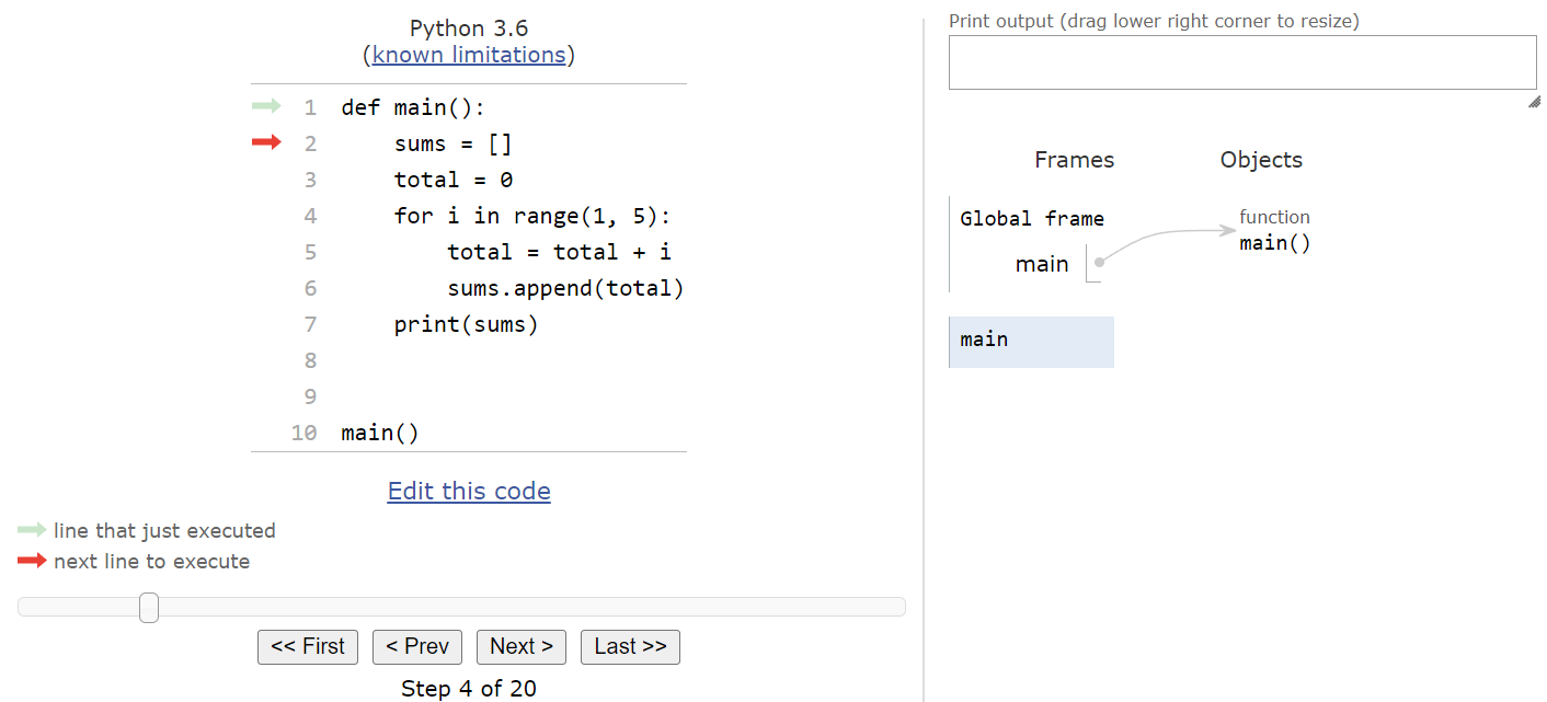
The very first line of code in the main() function will create a new list and store it in the sums variable. So, when we execute that line of code, we’ll see some new information appear in the frames and objects area in Python Tutor:
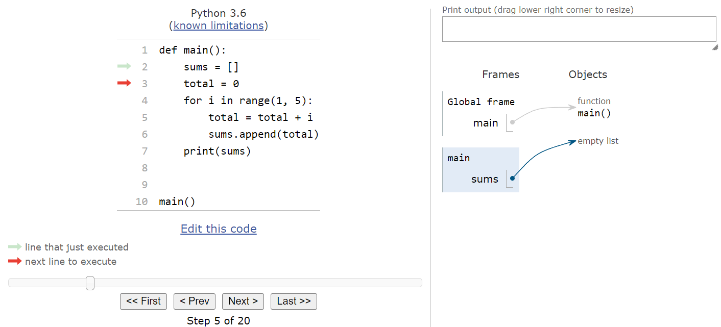
As we can see, in Python lists are treated like objects, so the sums variable in the main() function’s frame points to an empty list object in the objects list. As we add elements to the list, they’ll show up in the object itself. We’ll come back to this concept later in this lab to show why it is important to know that Python treats lists like objects instead of other variables.
The next line creates the total variable, setting it equal to $0$, and then we’ll reach the for loop:
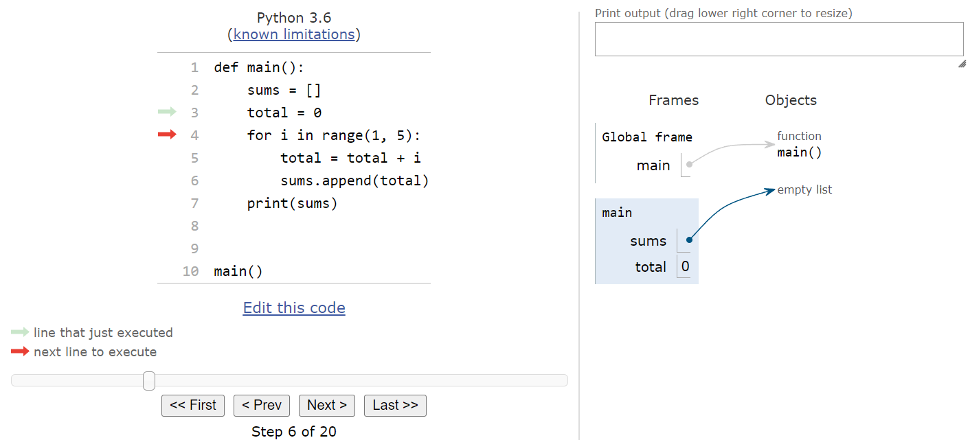
This for loop iterates four times, from $1$ up to but not including $5$. So, we’ll enter the loop with i storing the value $1$.
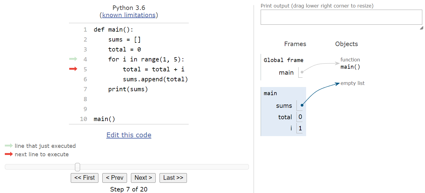
Inside of the loop, we’ll add the value of i to the total:

Then, we’ll append that new value in total to the end of the sums list. Since that list is empty, it will become the first item in the list, as we can see here:
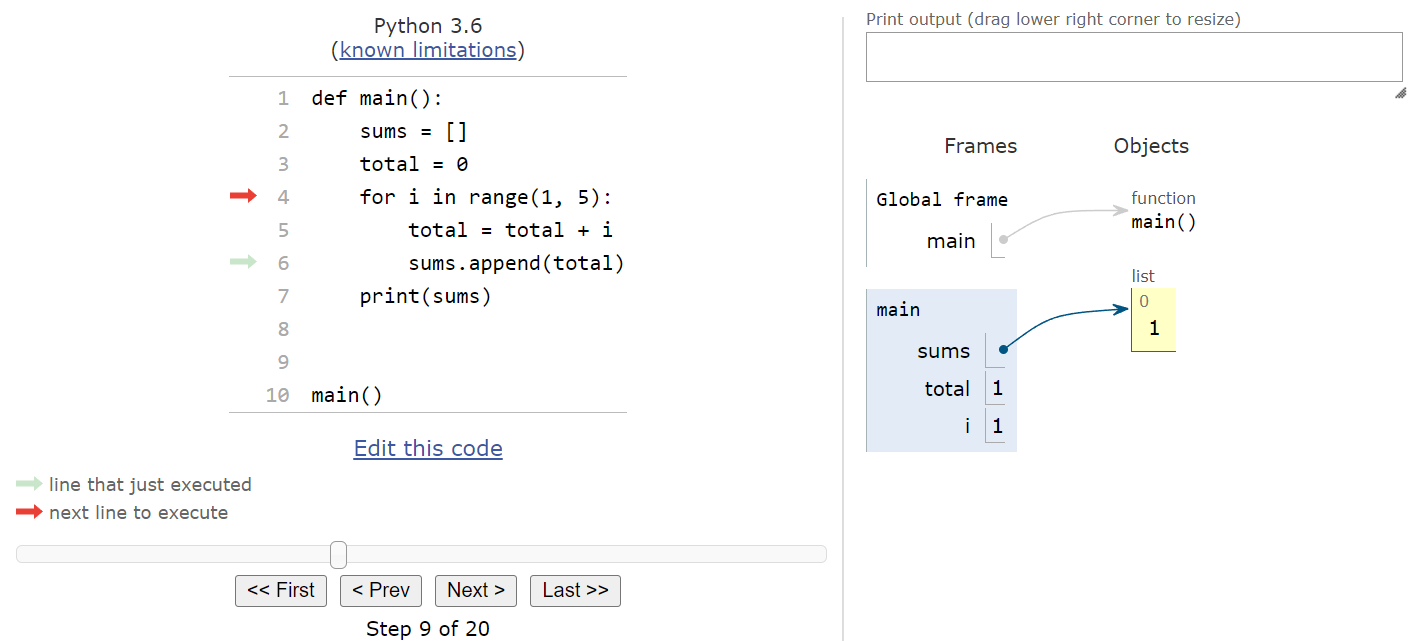
Notice that the list in the object area now includes a single element. On that element, we can see a small $0$ at the top of the box, which is the index of that element. Then, at the bottom and in a larger font, we see the value stored in that element, $1$. Just like with other variables, even though the assignment statement references the total variable, we are actually storing the value in the list, not a reference to the variable.
At this point, we’ve looped back to the top of the for loop, so we’ll increment i by one and enter the loop again:

Inside of the loop, we’ll add the new value of i to total, and then append that value to the sums list. After both of those steps, we should see the following state in Python Tutor:
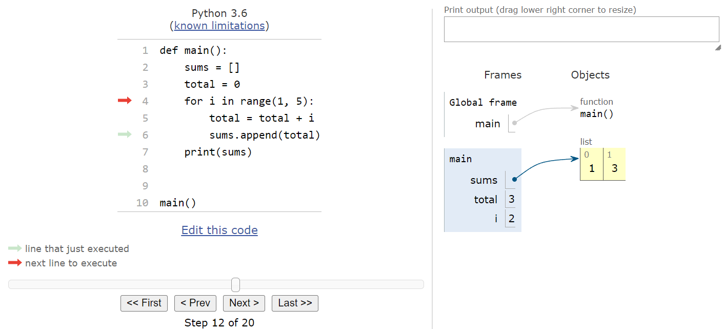
Notice that we now have two elements in the list. The first item, at index $0$, is still $1$, but now we’ve appended a second element at index $1$ that stores the value $3$. We’ve reached the top of the loop, so we’ll increment i and repeat those steps again. After the next loop iteration, we’ll see this state:
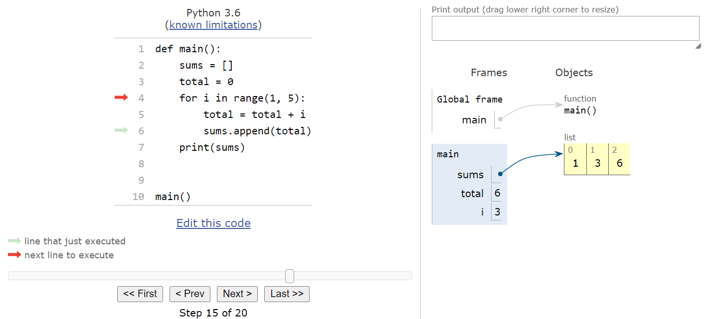
The process repeats one more time, leading to this state at the end of the for loop:
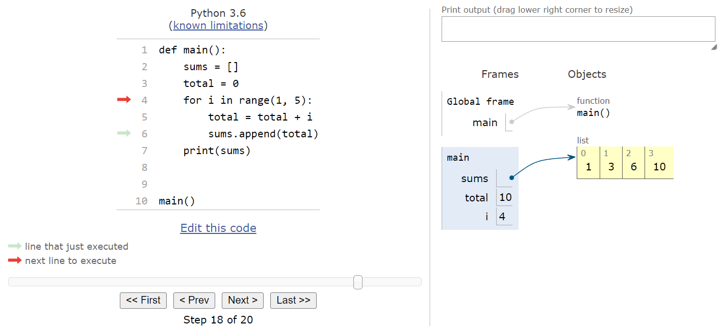
Notice that each time the loop iterates, we get a new value added to the sums list. Finally, we’re out of items to iterate over in the range, so we’ll jump to the bottom of the for loop and continue executing code from there:
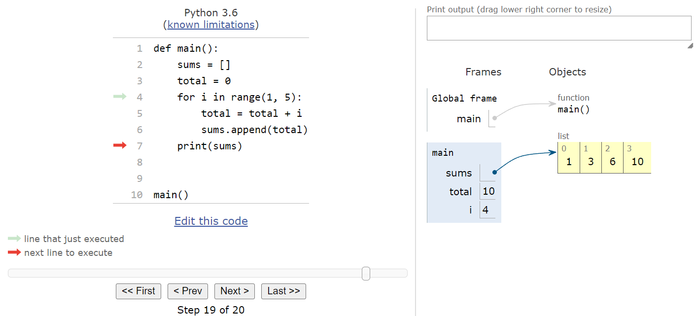
This last line of code will print the current contents of the sums list to the terminal. Python does a great job of formatting lists on the terminal so they are easy to read and understand. So, when we execute this line, we should see the following state, with output added in the print output section at the upper-right of the screen:
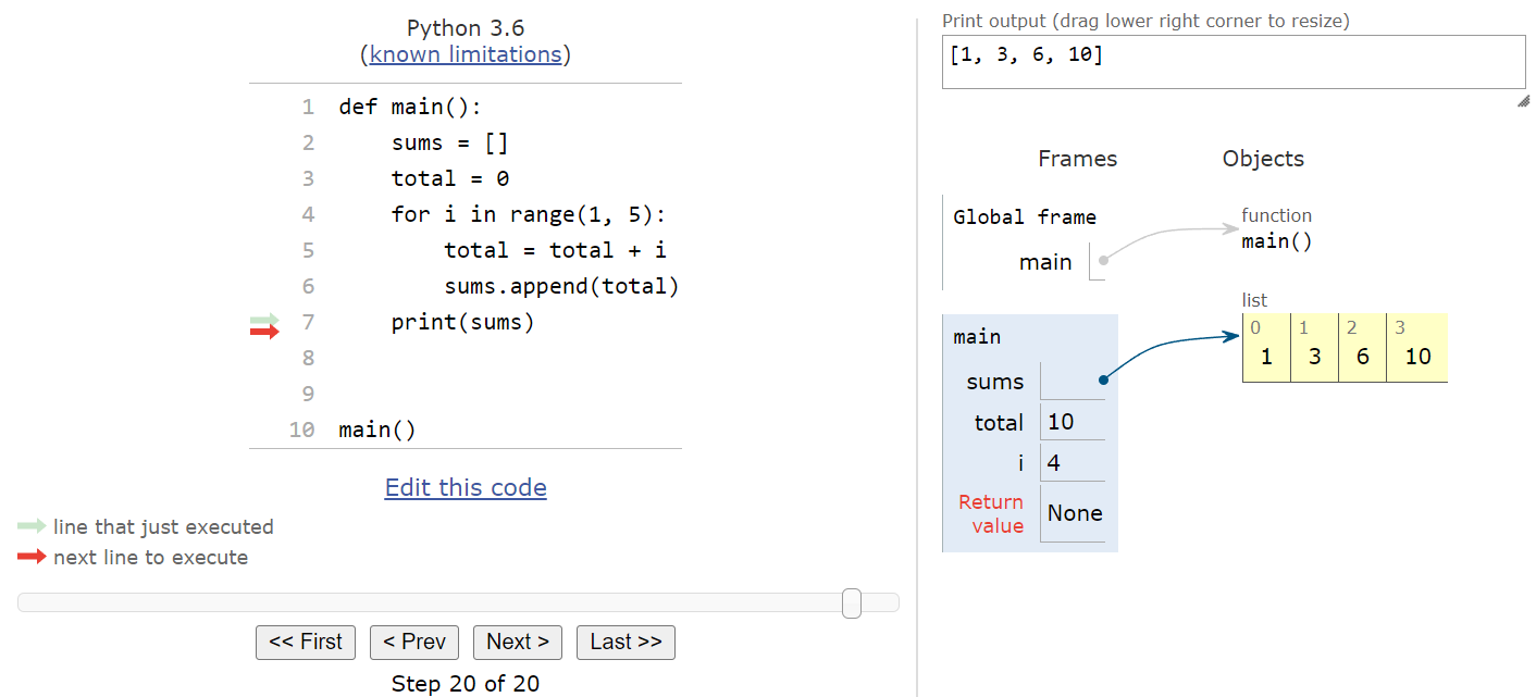
As we can see, adding elements to a list using a for loop works very easily, and Python Tutor does a great job showing us how Python will store that data in memory. The image below shows a full animation of this entire program.
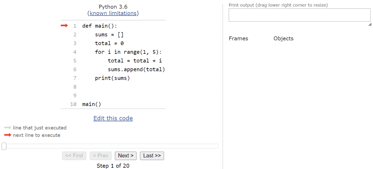
Later in this lab, we’ll see why this particular structure is used and why it is important.
One great way to work with lists in Python is using a loop. Recall from an earlier lab that a for loop actually iterates over a list itself, and that the range() function is simply used to generate a list that the for loop can use. Likewise, while loops can also be used in a similar way.
Let’s look at a quick example of how we can iterate through the items in a list using a loop in Python.
Consider the following example program in Python:
def main():
nums = [3, 1, 4, 1, 5, 9, 2]
print("The first seven digits of pi are...")
for i in nums:
print(i)
main()In this example, the for loop will iterate through the values in the nums list instead of a given range. So, during the first iteration, i will store the value $3$, then $1$, then $4$, and so on until it reaches the end of the list. When the program is executed, we should receive this output:
Using a list in a for loop is an excellent way to go through each element quickly, and it allows us to build for loops that don’t require the use of the range() function to generate a list that is in some sort of sequential order. We’ll see this pattern used very often in our programs using lists.
Finally, it is not recommended to edit the contents of the list while inside of the for loop using this method. Since we are only getting the individual values from each list element, we cannot easily make changes to the list itself without causing issues in the loop itself. Instead, if we want to make changes to the list while we are iterating through it, it is highly recommended to use a while loop structure as shown below.
It is also possible to iterate through a list in Python using a while loop. However, instead of iterating through the items themselves, we can use an iterator variable that references the indexes of the elements in the list. Consider this example program:
def main():
nums = [3, 1, 4, 1, 5, 9, 2]
print("The first seven digits of pi are...")
i = 0
while i < len(nums):
print(nums[i])
i = i + 1
main()This program is effectively the same as the one above, except that it uses a while loop to iterate through the items in the nums list. We start by setting the iterator variable i to be $0$, the first index in the list. Then, in the while loop, we use the special len() function, which is used to find the size of the list. Since the list contains seven items, the length of the list is $7$. Another way to think about the length of the list is that it is always one more than the highest index - if the last item in the list is at index $6$, then the length of the list overall must be $7$.
Then, inside of the loop, we’ll use the iterator variable i inside of square brackets to access each individual element in the nums list and print it to the terminal. We’ll also need to remember to increment i by one each time.
This method is very useful if we want to do more with the list inside of our loop, such as edit individual elements or make changes to the overall structure of the list. This works because we can directly manipulate the value in the iterator variable i, and then use it to access individual elements in the list and update them. Also, if the size of the list changes, it will be checked using the len() function after each iteration of the while loop.
So, as a general rule, we should use a for loop when we just want to iterate through the list and not make any changes to the list while inside of the loop. If we do need to make changes, it is better to use a while loop and an iterator variable to access the list elements directly.
Earlier in this lab, we saw Python Tutor create a list variable within the frame of a function, but that variable actually pointed to a list object that was stored in the global objects list. As it turns out, this seemingly minor distinction is a very important concept to understand how lists and functions interact with each other.
To demonstrate what is going on, let’s explore a program that contains multiple functions that operate on lists using Python Tutor once again. For this example, consider the following Python program:
def increment_list(nums):
i = 0
while i < len(nums):
nums[i] = nums[i] + 1
i = i + 1
def append_sum(nums):
sum = 0
for i in nums:
sum = sum + i
nums.append(sum)
def main():
nums = [1]
for i in range(4):
increment_list(nums)
append_sum(nums)
print(nums)
main()Before we go through the full example, take a minute to read through the code and try to piece together how it works. For example, notice that the increment_list() and append_sum() functions do not return a value! Since they don’t return a value, will they really have any impact on the program itself?
To find out, let’s run through this program in Python Tutor. As always, you can copy the code to the tutor.py file in Codio, or click this Python Tutor
link to open it in a web browser.
Python Tutor begins by adding all of the functions to the global frame, and then entering the main() function when it is called at the bottom of the code. Once the program enters the main() function, we should see this state:
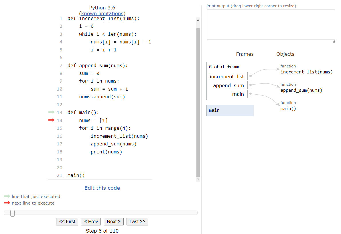
The main() function begins by creating a single list in the nums variable, which initially stores a single element, the number $1$. So, we’ll see the nums variable added to the main() function’s frame, with a pointer arrow to the list itself in the list of objects to the right:
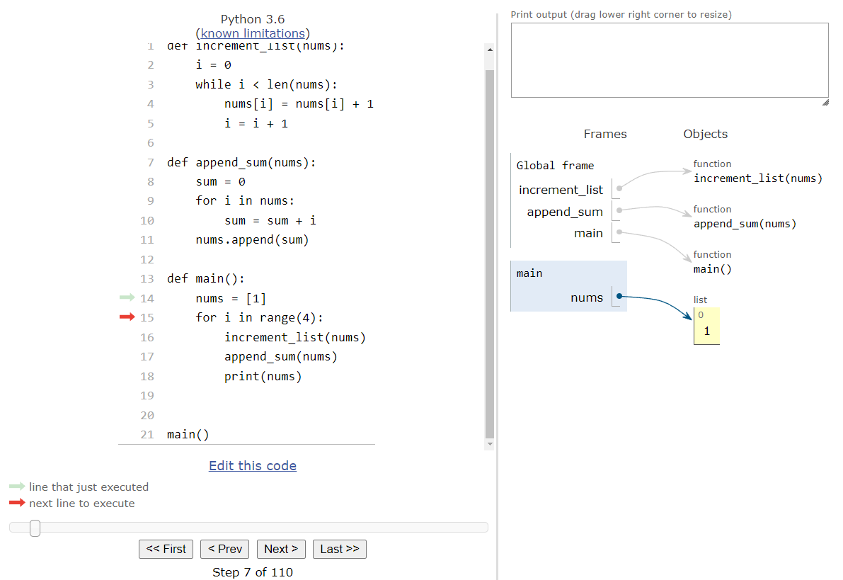
Next, we’ll reach a for loop that will iterate $4$ times. So, we’ll store the first iterator value, $0$, in the iterator variable i and enter the for loop:
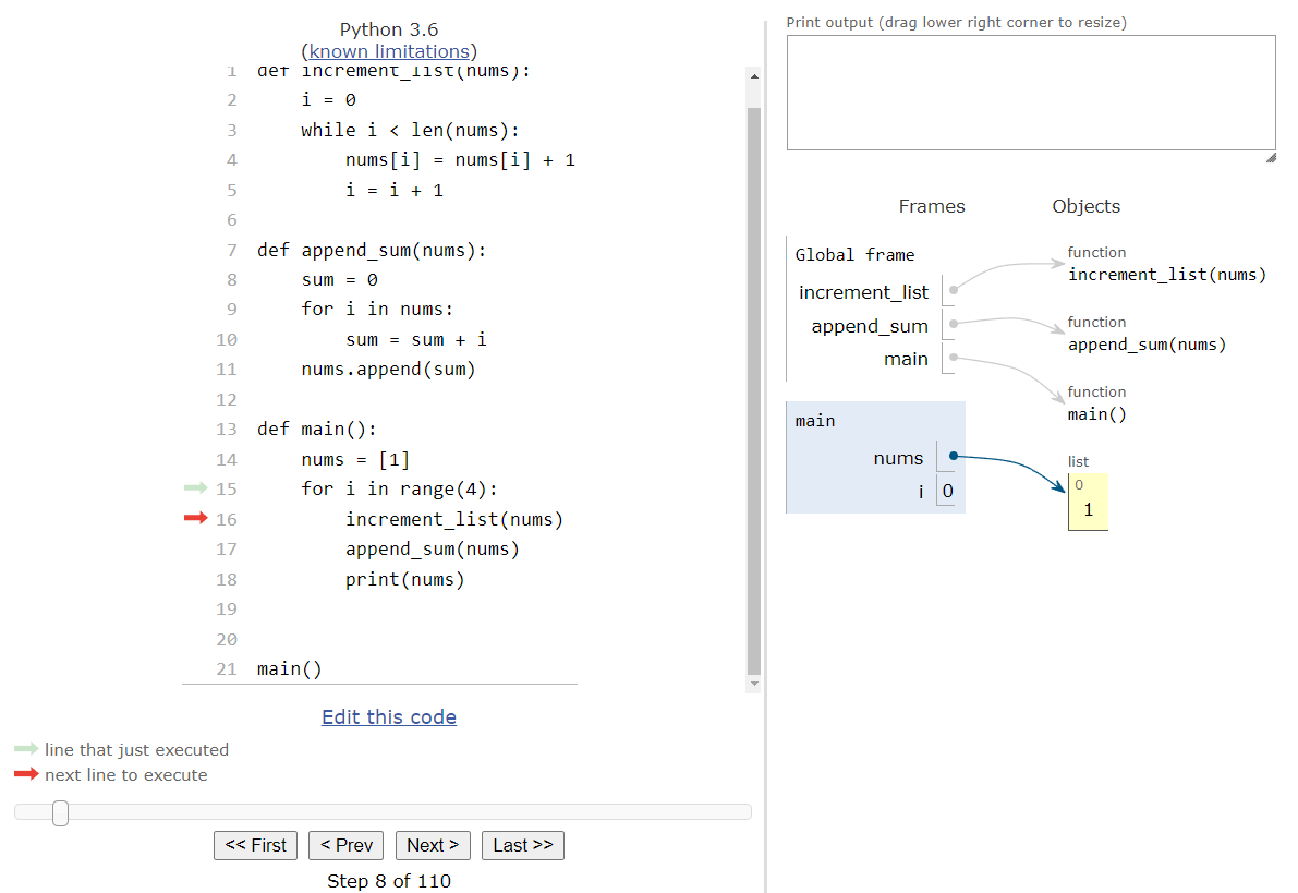
Inside of the for loop, the first step is to call the increment_list() function, which accepts a single parameter. So, we’ll provide the nums list as an argument to that function call. Just like always, Python Tutor will create a new frame for the increment_list() function when we call it, and it will populate all of the parameters for that function with the arguments that are provided, as shown here:
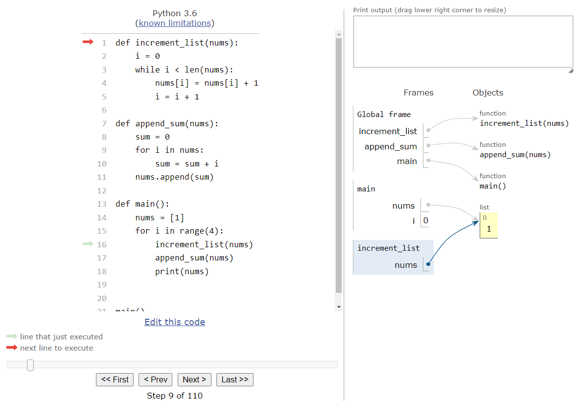
In this state, we see something interesting. In the increment_list() frame, we see the parameter nums is also a pointer to a list, but notice that it points to the exact same list object that the main() frame points to. This is because we are only sending the pointer to the increment_list() function so it knows where to find the list in the objects in memory, but it doesn’t actually duplicate the list.
In programming, we call this method of dealing with parameters call by reference, since we are simply passing references, or pointers, to the various objects but not the objects themselves. In technical terms, we’d say that the list is a mutable, or changeable, object, so we’ll use call by reference instead of the usual call by value process.
The next step will be to enter the increment_list() function itself:
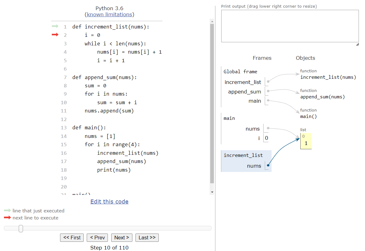
In this function, we are getting ready to use a while loop to iterate through the nums list. Since we’re going to be editing the values stored in the list, we should use a while loop instead of a for loop. So, we’ll start by setting the initial value of our iterator variable i to $0$, and then we’ll reach the while loop in code:
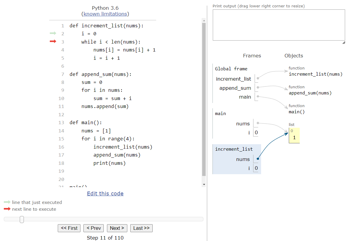
When we’ve reached the while loop, we’ll need to make sure that our iterator variable is less than the size of the list. Since i is currently storing $0$, and our list contains at least one item, this Boolean expression is True and we’ll enter the loop:
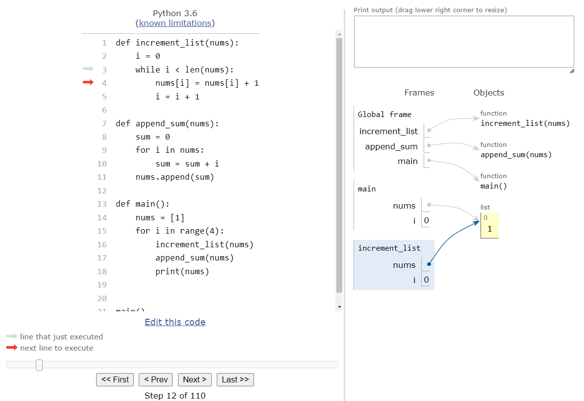
Inside of the loop, our goal is to increment each item in the list by $1$. So, we’ll use the iterator variable i inside of square brackets to both access the item in the list currently on the right-hand side of the assignment statement, and then we can also use it as the location we want to store the computed value, which is on the left-hand side of the assignment statement.

Then, we’ll increment our iterator variable i by $1$, and then jump back to the top of the loop:

At this point, we must check our Boolean expression again. This time, our iterator variable i is storing $1$, but the length of the list is also $1$, so the Boolean expression is False and we should skip past the loop. Since there is no additional code in the increment_list() function after the loop, the function will simply return here.
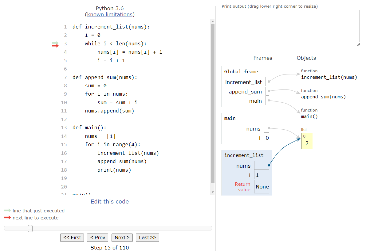
Notice that the function itself is not returning a value. Since Python uses call by reference, we don’t have to return the nums list back to the main() function even though we updated it, because the main() function still has a pointer to that exact same list object in memory. So, once the function returns, we’ll end up back in the main() function as shown here:
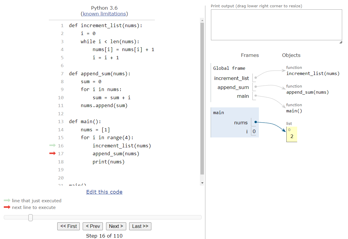
Notice that the frame for the increment_list() function is now gone, but the changes it made to the list are still shown in the list object to the right. This is why working with lists and functions can be a bit counter-intuitive, since it works completely differently than single variables such as numbers and Boolean values. A bit later in this lab, we’ll discuss how string values can be treated as lists, even though they are technically stored as single variable values.
The next step in this program is to call the append_sum() method, using the same nums list as before. So, we’ll create a new frame for that function and populate it once again with a pointer to the nums list in memory - the very same nums list that the main() function is using:
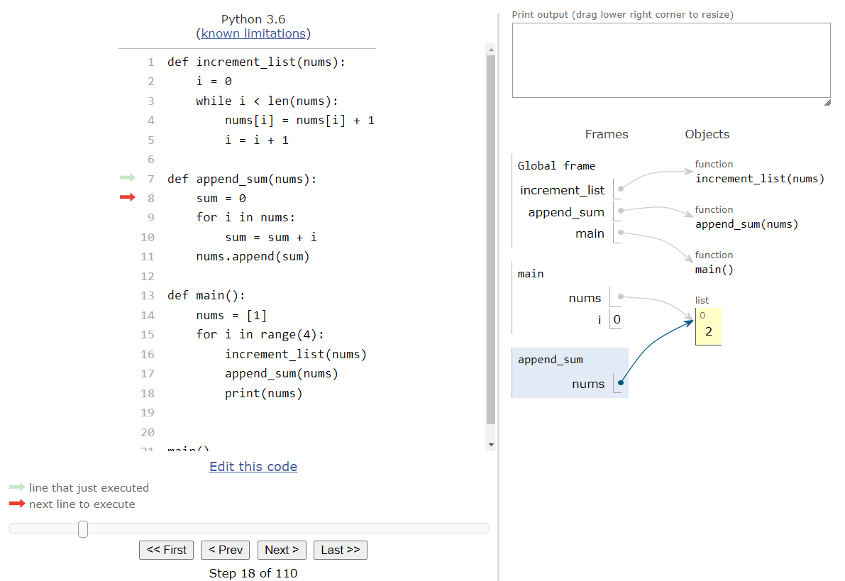
In the append_sum() function, our goal is to sum up all of the values currently in the list, and then append that value to the end of the list. So, we’ll need to create a sum variable to keep track of the total, which will initially store $0$:
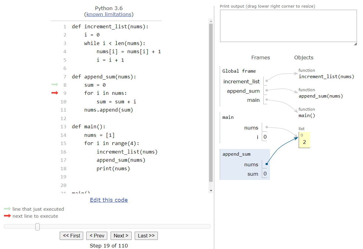
Thankfully, since we are not going to update the list from within our loop, we can use a simple for loop to iterate through the list. So, we’ll start by storing the first value in the list, $2$, into our iterator variable i, and then we’ll enter the loop.

Inside of the loop, all we are doing is adding the value currently stored in i to the sum variable. So, we’ll store $2$ in sum and jump back to the top of the loop.

At this point, we’ve used every element in the list in our loop, so the loop will terminate and we’ll jump down to the code directly below the loop as shown here:
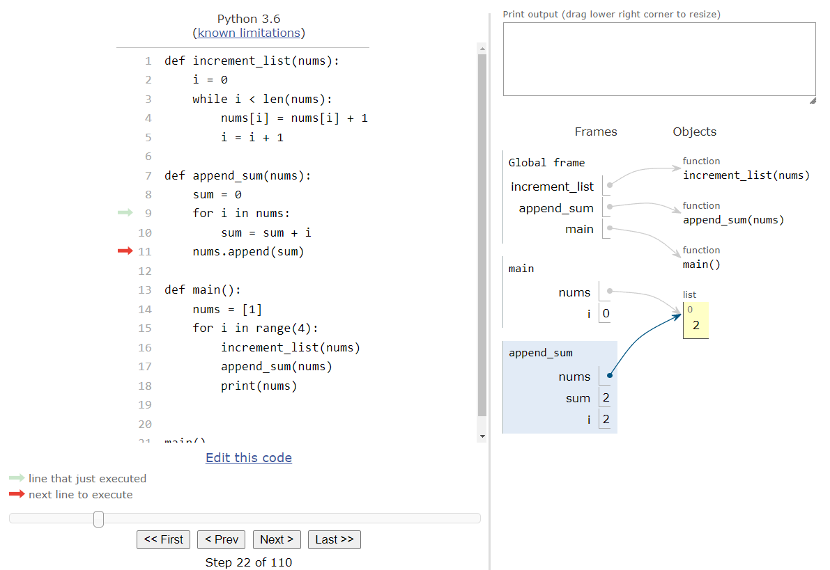
Finally, the last line of code in this function will append the value of sum to the end of the list.
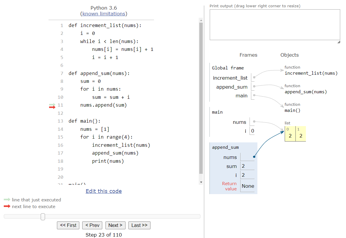
At this point, we’ve modified the list to contain a new element. However, in Python Tutor we can clearly see that this item was just added to the existing list object in memory. So, when we get back to the main() function, we’ll be able to access the existing list, which will now include this new element as well.
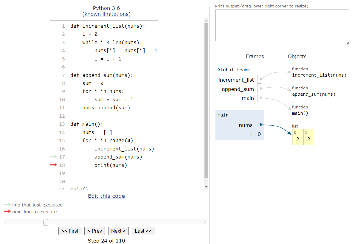
Back in the main() function, the last step in the loop is to print the current contents of the list to the terminal. So, after we execute that line, we should see some output in our print output box at the top right of the screen:

There we go! That’s one whole iteration through the loop in the main() function. This process will repeat $3$ more times. Each time, we’ll first increment the elements in the list using the increment_list() function, as shown here:
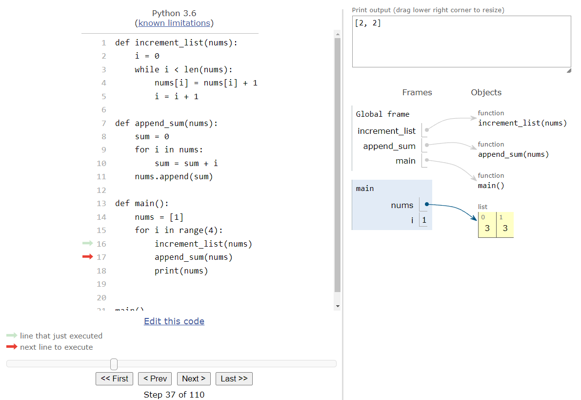
Then, we’ll sum up the existing elements in the list and append that value to the end of the list, which will result in this state:
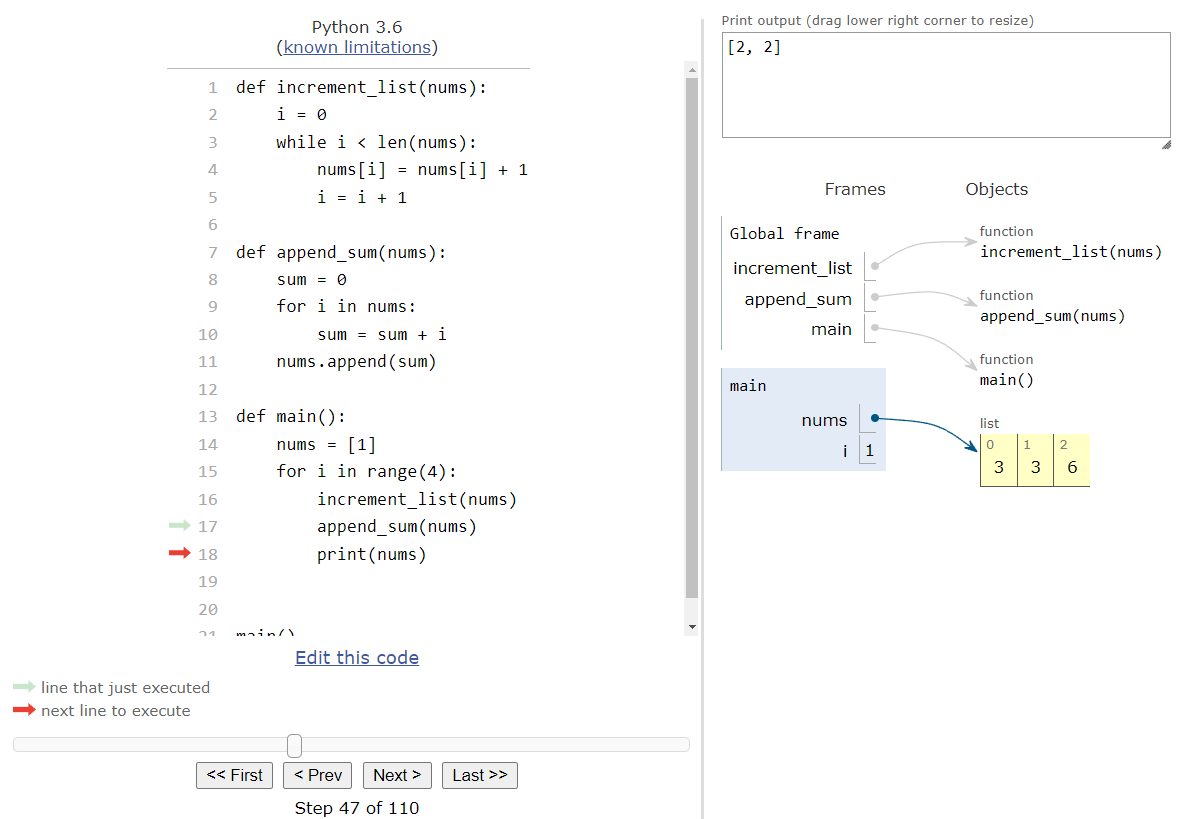
Finally, we’ll print the contents of the list at that point, and jump back to the top of the loop:
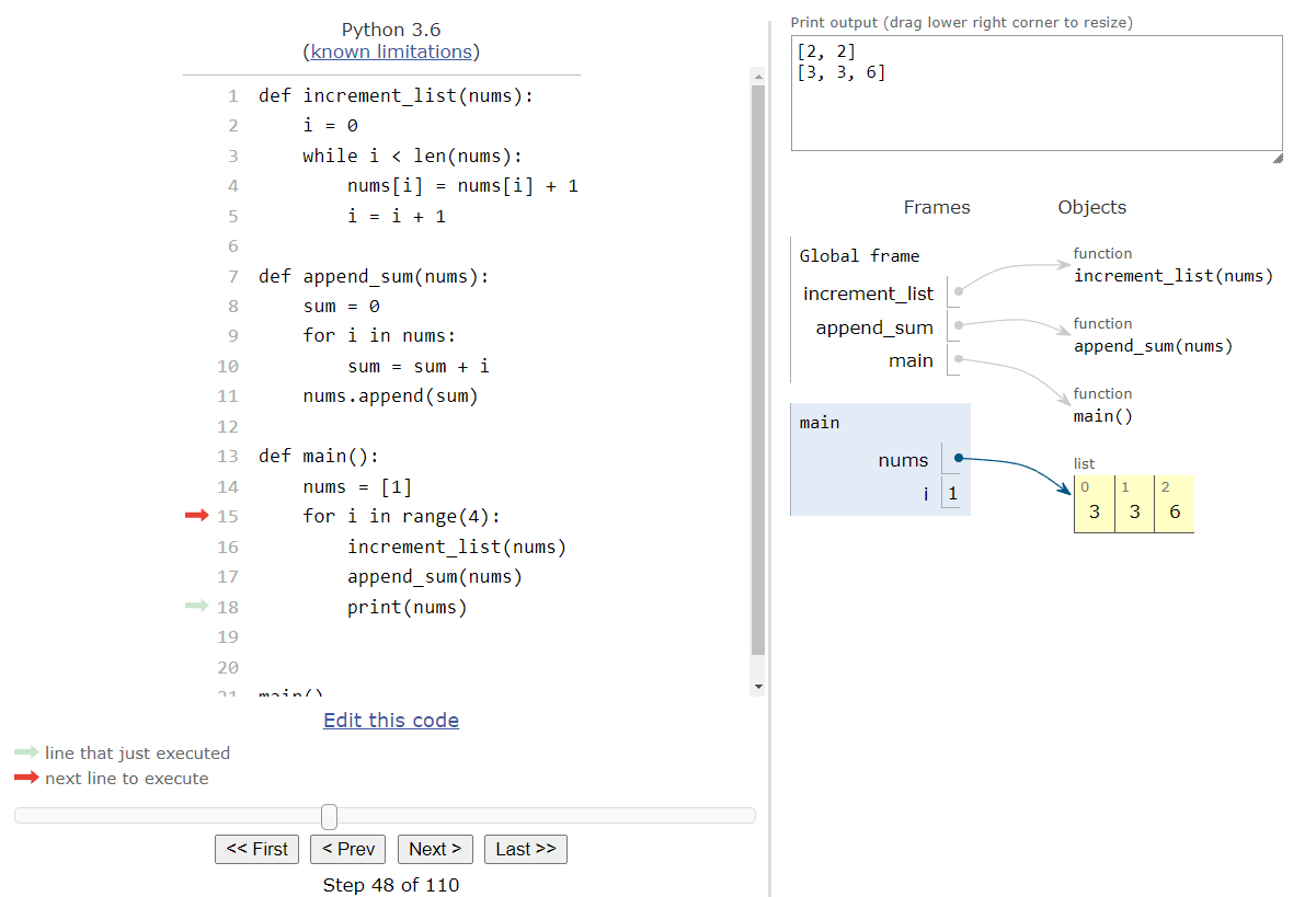
Each time, the list will be updated by the various functions that the main() function calls. Thankfully, since Python uses call by reference, each function is able to update the same list object in memory, making it quick and easy to work with lists and functions in Python. At the end of the entire program, we’ll see this state:
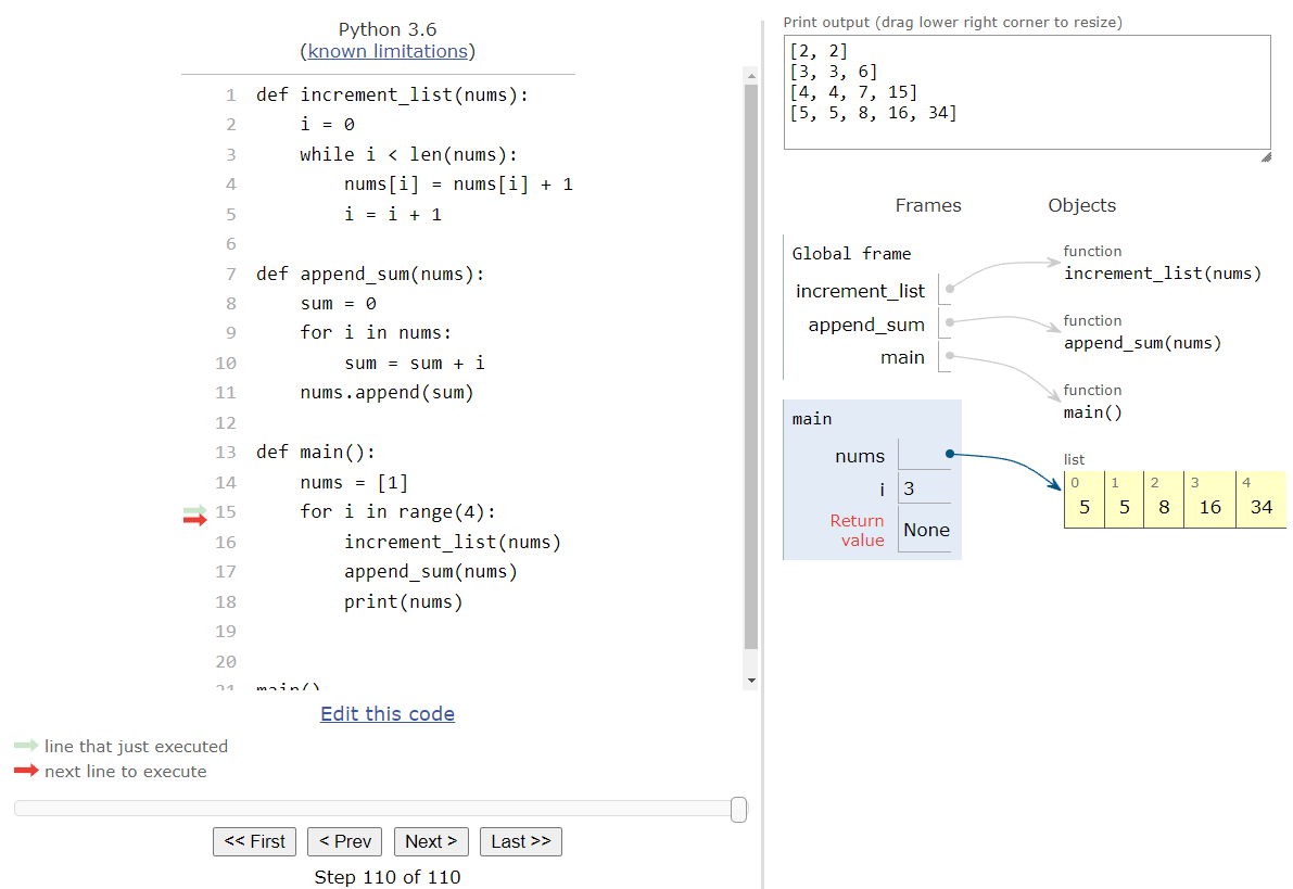
A full animation of this program, with some steps omitted, is shown here:
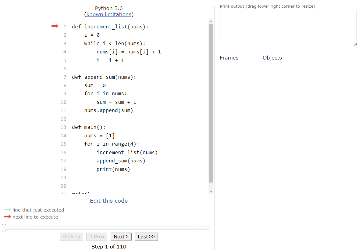
Functions that use lists as parameters are a very common technique in programming, and it is very important to understand how they work. If we aren’t careful, it is very easy to make a change to a list inside of a function call, and then later assume that the original list is unchanged. Likewise, if we pass a list as an argument to a function that works differently than we think it should, it could end up changing our data without us even noticing it. Hopefully this example makes it very clear how Python functions handle lists as parameters.
One of the coolest features in Python is the ability to easily create slices of lists. A slice is simply a portion of a list that can be stored and used as a separate list, allowing us as programmers to quickly create and manipulate new lists based on existing lists.
There are two basic ways to create a list slice in Python.
nums[start:end] - this will create a slice of the list stored in nums that begins as the index start and ends before the index end. For example, if nums is storing the list [2, 4, 6, 8, 10], then nums[1:3] would create the list slice [4, 6].nums[start:end:step] - this will create a slice of the list stored in nums that begins as the index start, moves step indexes between each successive items, and ends before the index end. For example, if nums is storing the list [2, 4, 6, 8, 10], then nums[0:5:2] would create the list slice [2, 6, 10].The method for creating list slices is very similar to how the range() function is used in Python. In effect, if the same values are provided as arguments to the range() function, then it will produce the list of indexes that will be used to generate the list slice.
Beyond the simple syntax, there are a few other rules to understand about list slices:
start will be $0$ at the start of the list, end will be the size of the list, and step will be $1$. So, each of these are valid ways to slice a list, and there are many more possible combinations:
nums[:] - this will effectively copy the list and include every item in the slice.nums[start:] - this will include all items in the list starting at start.nums[:end] - this will include all items in the list before end.nums[::step] - this will include all items in the list starting at index $0$ and moving forward step indexes eachnums[-1] - this will access the last item in the listnums[-3:] - this will create a slice containing the last three items in the list.nums[:-2] - this creates a slice of the entire list except for the last two items.For example, we can start with a simple list, and then try the various list slicing methods to see what elements would be included in the new list. Here’s an example program that shows some of the various ways to manipulate lists in Python:
def main():
nums = [0, 1, 2, 3, 4, 5, 6, 7, 8, 9]
print(nums)
# simple slices
print(nums[3:7])
print(nums[5:])
print(nums[:5])
print(nums[::2])
print(nums[1::2])
# negative numbers
print(nums[-1])
print(nums[-7:-3])
print(nums[-3:])
print(nums[:-3])
print(nums[::-1])
main()When we execute the program above, we should see the following output:
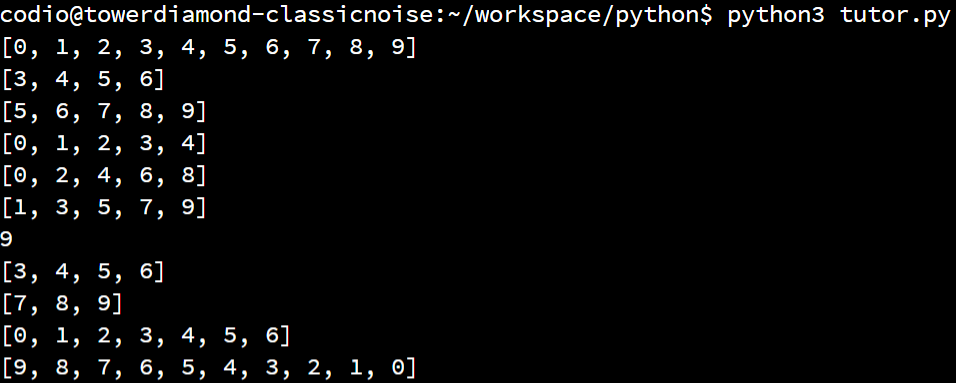
List slicing is a great way to use and manipulate lists in Python, but it takes a bit of practice to learn all the various ways that it can be used. Feel free to play around with all of the various examples above using some sample data to see how they work.
The range() function in Python is used to generate a list, but unfortunately we can’t directly use that list in our code without a bit of manipulation. For example, we can try to store the result of the range() function in a variable as shown here:
nums = range(10)
print(nums[3:7])However, when we try to run that code, we’ll see this output:
range(3, 7)This is because the range() function doesn’t actually create a list - it is it’s own data structure type! Since a range can be constructed from just three numbers, it is much simpler to store just those numbers in memory instead of the entire list of numbers that it represents. When we create a slice of a range object, it just generates a new range instead of a list. So, to actually convert a range to a list, we must use the list() function in Python:
nums = list(range(10))
print(nums[3:7])This will produce the expected output:
[3, 4, 5, 6]You can learn more about this by reading Python’s Range documentation.
Throughout this course, we’ve seen several different ways to work with strings. In Python, just like in many other programming languages, it is possible to treat strings as a list of individual characters. Because of this, we can write many useful programs that use and manipulate strings in a variety of ways.
Let’s look at one quick example program that can manipulate strings just like a list! Consider the following Python program:
import random
import string
def encode(secret, step):
output = ""
for i in secret:
output = output + i
for j in step:
output = output + random.choice(string.ascii_lowercase)
return output
def decode(code, step):
return code[::step]
def main():
secret = input("Enter a secret word")
step = int(input("Enter a positive integer"))
code = encode(secret, step)
print("Your code is:")
print(code)
print()
decoded = decode(code, step)
print("I can decode it back to:")
print(decoded)
main()This is a very simple encoding program that will allow the user to enter a secret phrase, encode it by inserting many random characters between the characters of the word itself, and then show that it can be decoded once again. This is very similar to how a Scytale encodes messages.
Let’s briefly walk through this example using Python Tutor to see how it works. As always, we can copy and paste this code in the tutor.py file in Codio, or click this Python Tutor
link to open it in a browser window.
We can skip ahead to the point where the code enters the main function, as shown in this state:
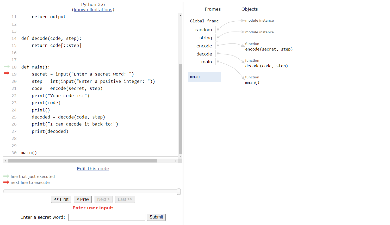
Let’s assume that the user inputs the string "password" for the secret word. That will be stored in the secret variable. On the next line, we’ll ask the user to input a positive integer:
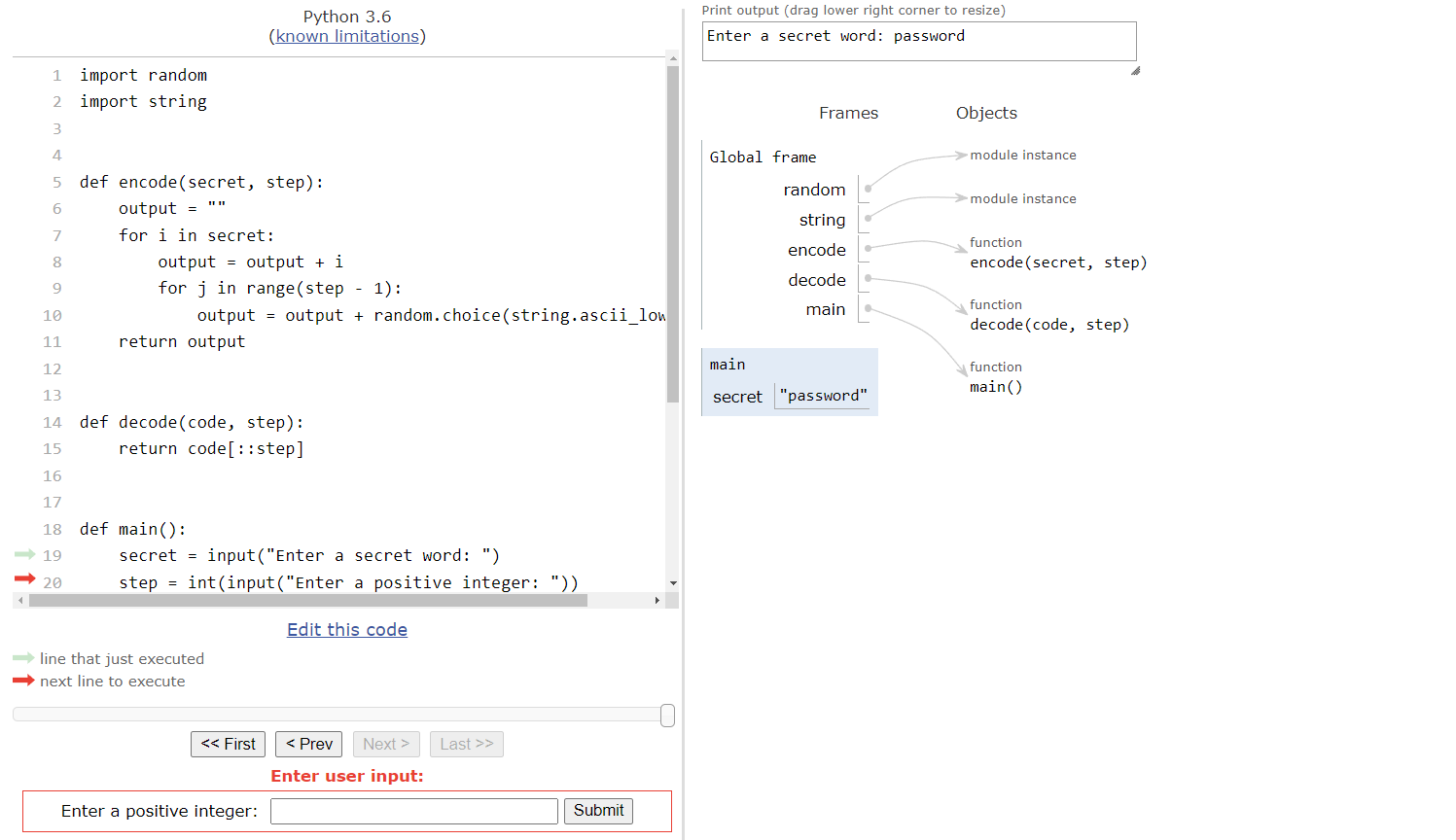
For this input, we’ll assume the user chooses to input the number $5$. So, we’ll store that in the step variable in our main() function, as shown here:
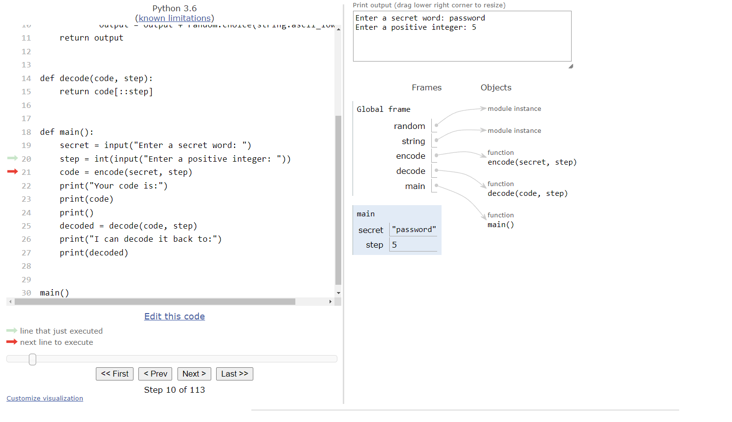
At this point, we’re ready to call the encode() function, which requires two parameters. We’ll use the variables secret and step as the arguments to those parameters, so Python Tutor will create a new frame for the encode() function and store those values within it:
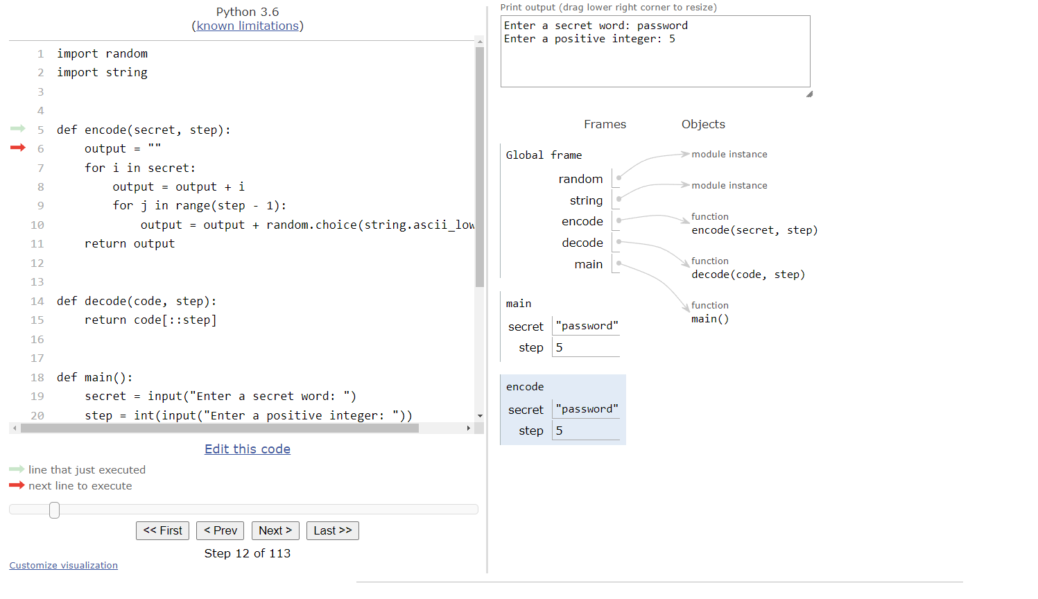
At this point, we can notice one very important difference between strings and lists. Even though a string can be treated like a list, as we’ll see in this example program, it is still stored as a single variable item in the frame. So, the encode() function’s frame now contains a copy of the string secret, not a pointer to the original variable in the main() function’s frame. Technically, we would say that strings are an immutable data type, so we cannot change them from within a function like we can do with lists.
Inside of the encode() function, we’ll start by creating a new variable output, which is initially set to store an empty string.
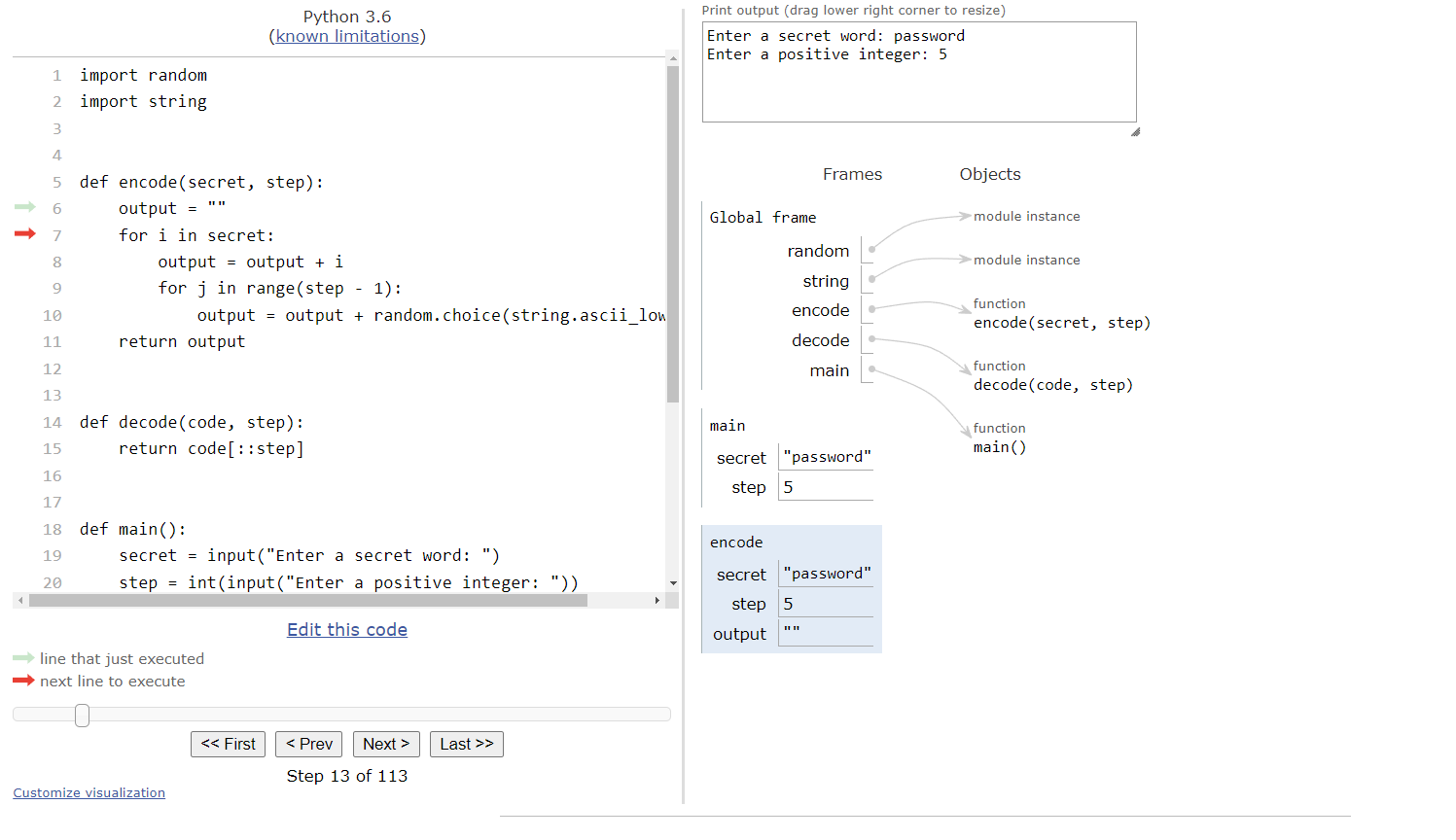
Then, we’ll reach a for loop. This for loop will iterate through each character in the secret string, one at a time. So, just like with a list, each character will be stored in the iterator variable i so we can use it inside of our for loop. For the first iteration, we’ll store the character 'p' in the iterator variable i, then we’ll enter the loop:

Inside of the loop, the first step is to append the current iterator variable i to the output string. So, we’ll place the character 'p' at the end of that string:
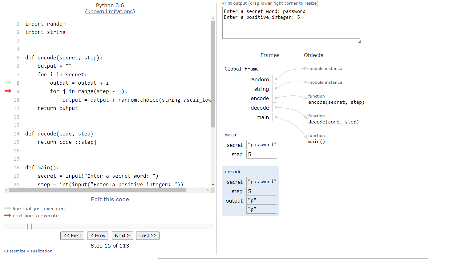
Then, we’ll reach a second for loop. This loop will repeat step - 1 times, so we’ll enter the loop and set the iterator variable j to be $0$ initially.

Inside of this loop, we have one complex line of code that we haven’t seen before. First, we have the string.ascii_lowercase list, which is a built-in list that is part of the string library which contains all $26$ lowercase letters of the English alphabet. To use this list, we have to include the import string line at the top of our file. Then, we use a special function named random.choice(), which is used to choose a random element from a list. So, we’ll also have to include the import random line at the top of our file to use that library as well. Finally, we’ll add that character to the end of the output string.

We’ll repeat this process a few more times. Once we exit the innermost for loop, we should be at this state:
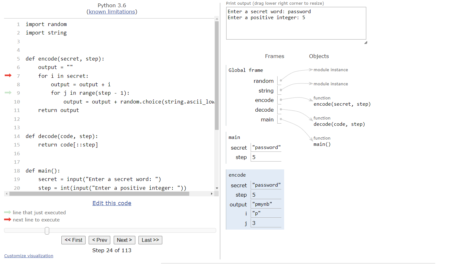
In the output variable, we now see the first character of our secret word, 'p', followed by four random characters. These random characters make it more difficult for someone to decode our message. We’ll repeat this process for each of the other letters in our secret word. So, at the end of the encode() function, we should be at this state:
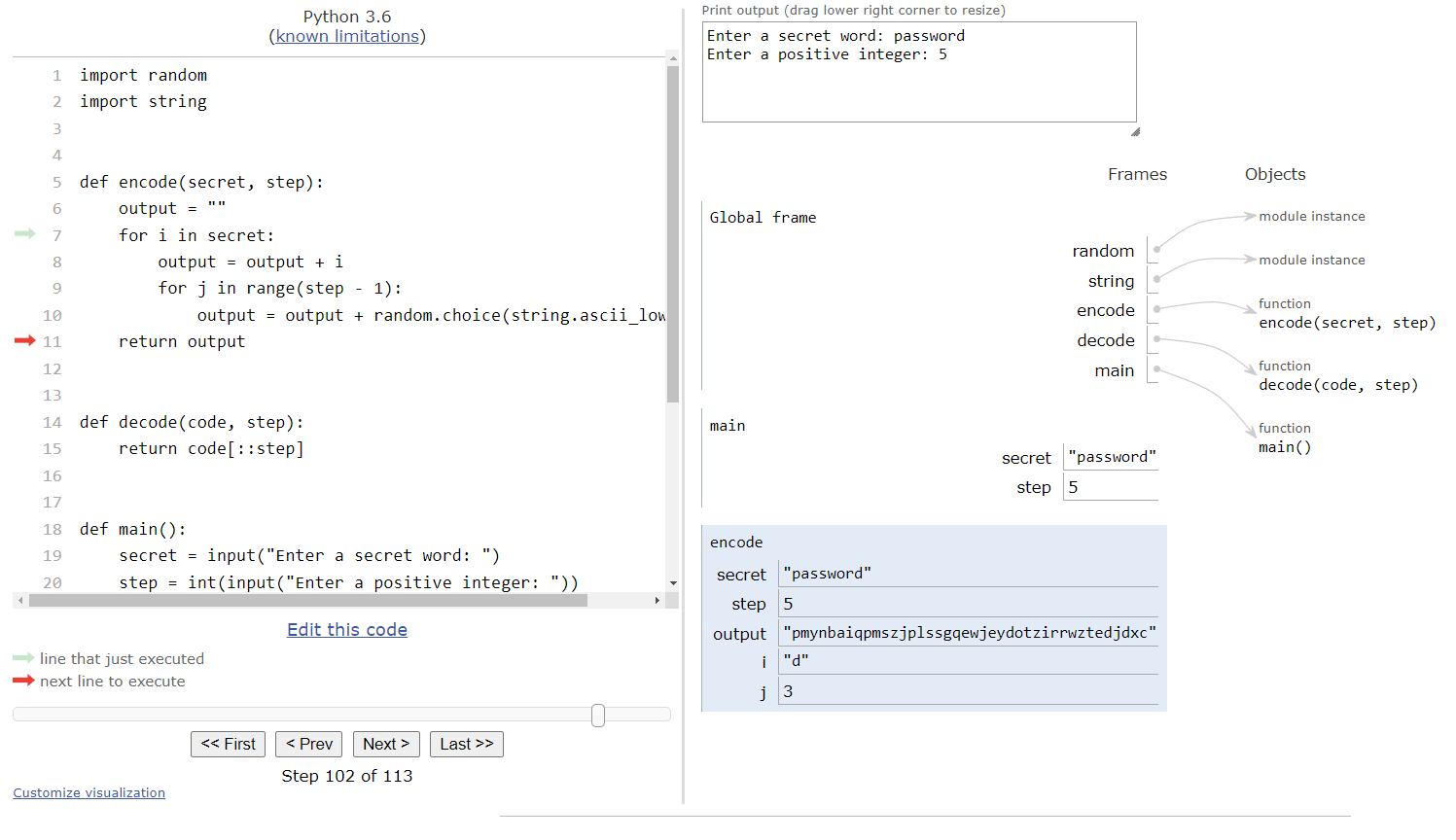
As we can see, the output variable appears to be completely random at first glance, which is exactly what we want. At this point, the encode() function will return that string back to the main() function, and it will be stored in the code variable there.
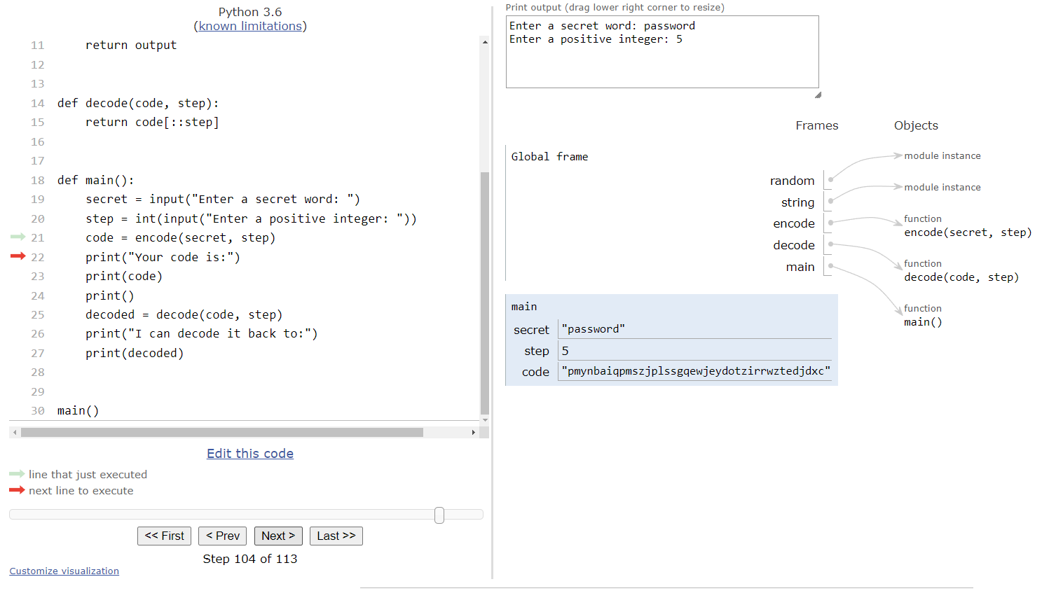
Next, the main() function will print out some helpful output, and then eventually it will reach the line that calls the decode() function.
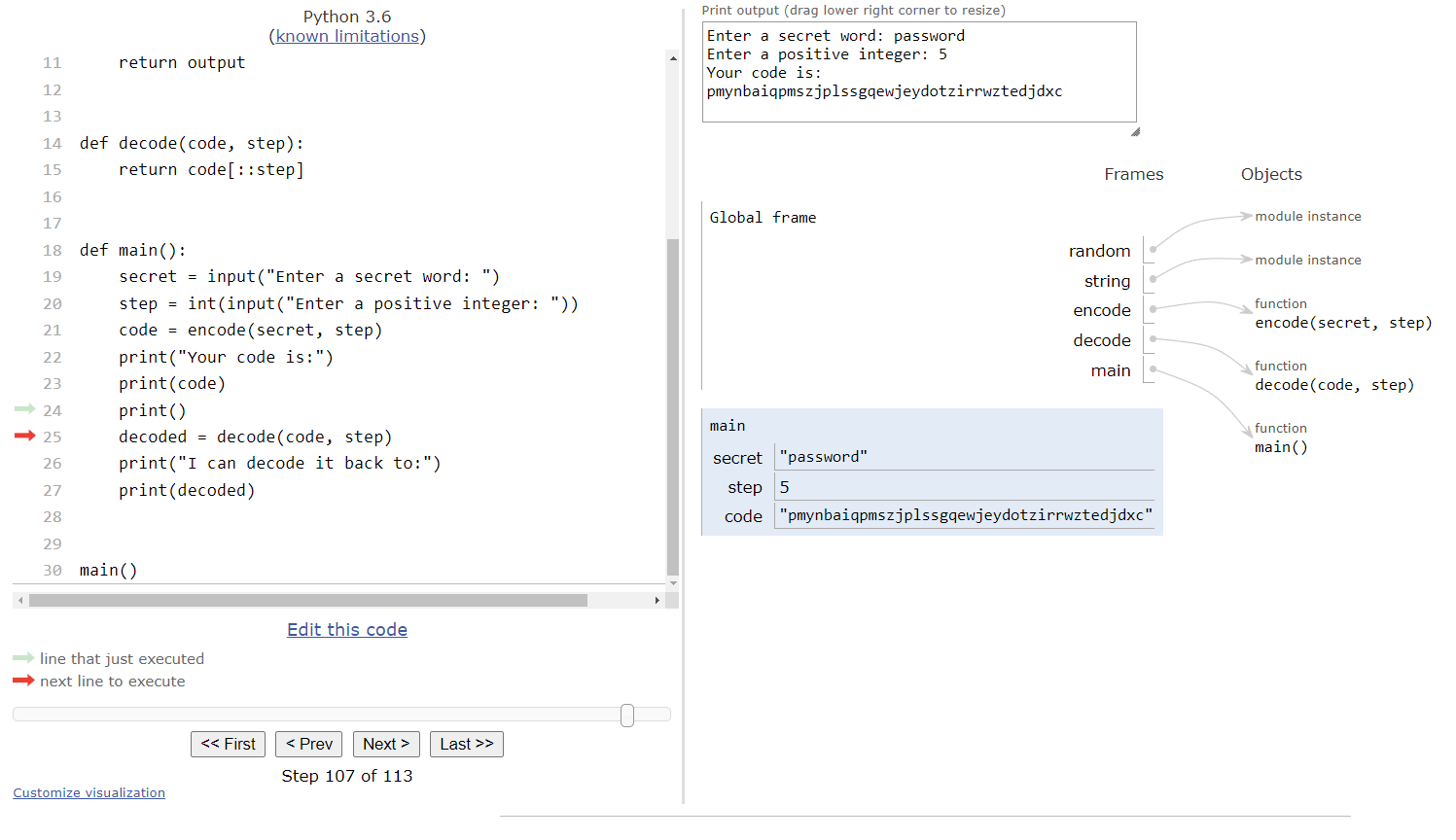
Once again, we’ll copy the values in the code and step variables to the decode() function’s frame since they are provided as arguments, and then we’ll enter the decode() function:
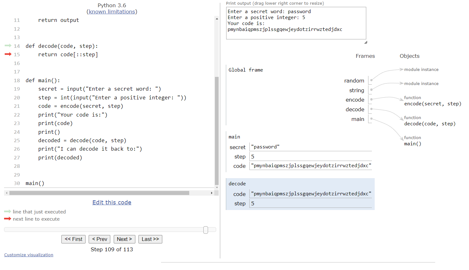
In this function, we see that we can decode our encoded phrase using a simple slicing operation, with the step variable providing the key we need to get our secret word out of the encoded string. We’ll return that back to the main() function:
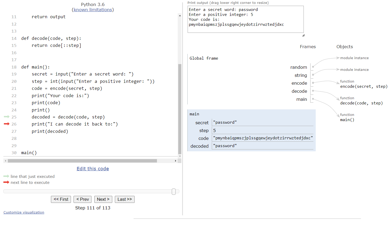
There we go! We’ve shown that we can easily construct an encoded phrase in a string using a secret word and a step variable, and then we can decode that phrase using a simple string slice. At the same time, we were able to explore how strings can be used like lists by iterating through a string and creating slices of a string, but also that strings are immutable and aren’t passed using call by reference like lists are. Instead, strings use call by value in Python, so we have to remember to return our updated strings at the end of any functions that manipulate them.
Thankfully, being able to work with strings in Python using the same methods as lists makes it very easy to write a wide variety of programs that create and manipulate strings!
Finally, let’s work through another full example program in Python that uses lists and strings, just to gain some more experience with the various ways we can use the techniques we’ve learned in this lab.
For this example, consider the following problem statement:
Write a program to construct and print Pascal’s Triangle for a given number of rows. The user should be prompted to enter a positive integer indicating the number of rows, and if the user provides an invalid input the program should prompt for additional input until valid input is received.
Pascal’s Triangle is a simple mathematical construct that begins with the value $1$, and then each value below on the triangle is the sum of the two values immediately above it. The first few rows of Pascal’s Triangle are shown below:
1
1 1
1 2 1
1 3 3 1
1 4 6 4 1We can easily do this with loops and lists. So, let’s go through the process of building that program from scratch.
To begin, we can start with our usual program structure consisting of a main() function and a call to the main() function at the bottom of the file:
def main():
main()Next, we’ll include the positive_input() function that we’ve used in several previous labs, which handles prompting the user for a positive integer input and will prompt the user for additional input if an invalid value is provided. Once again, we’re doing our best to reuse pieces of code we’ve already written:
def positive_input():
x = int(input("Enter a positive integer: "))
while x <= 0:
print("Invalid input!")
x = int(input("Enter a positive integer: "))
return x
def main():
main()In our main() function, we can quickly call the positive_input() function to get the required piece of input from the user and store it in the variable n:
def positive_input():
x = int(input("Enter a positive integer: "))
while x <= 0:
print("Invalid input!")
x = int(input("Enter a positive integer: "))
return x
def main():
n = positive_input()
main()That’s the basic structure of our program to handle input. It’s very simple and mostly reused code, so it should be quick and easy to get to this point of our development process.
Next, we should add some of the initial steps to our program. For example, we know that the first row of Pascal’s Triangle is simply the number $1$, so we can create an initial list that contains just that single element, and then print that to the terminal:
def main():
n = positive_input()
row = [1]
print(row)Next, we know we need to create additional rows of Pascal’s Triangle, up to n rows in total. So, we can quickly build a for loop that will handle that in our main() function:
def main():
n = positive_input()
row = [1]
print(row)
for i in range(1, n):
# update row
print(row)Notice that we are starting our range at $1$ instead of $0$. This is because we’ve already printed the first row, so we only want to print additional rows if the value of n is greater than $1$. That’s the basic structure we need in our main() function
Finally, we need to deal with the process of updating our row list to include the next row’s information. While we could do that directly in the main() function, it makes the most sense to create a separate method for that. So, we’ll start by creating a new function update_row() that requires a single parameter:
def update_row(row):In this function, we need to use the previous row on Pascal’s Triangle to compute the next row. This is a bit tricky to figure out, but thankfully there are a few helpful rules that we can follow:
i+1 of the new row is the sum of the items at index i and i+1 on the previous row.Using those rules, we can write a loop in code that will create a new list for the next row. First, since we’ll be using multiple items from the row list in our loop, we’ll need to start with the generic while loop structure to iterate through the list:
def update_row(row):
i = 0
while i < len(row):
# use list elements
i = i + 1We can also initialize our new list to start with the value $1$ initially:
def update_row(row):
i = 0
new_row = [1]
while i < len(row):
# use list elements
i = i + 1Inside of the while loop, we can append new items to our new_row by simply summing the elements at index i and i + 1 of our previous list:
def update_row(row):
i = 0
new_row = [1]
while i < len(row):
new_row.append(row[i] + row[i + 1])
i = i + 1At the end, we’ll need to add the final $1$ to the new row. Finally, since we’re creating a new list instead of modifying the existing one, we’ll need to return that reference back to the main function:
def update_row(row):
i = 0
new_row = [1]
while i < len(row):
new_row.append(row[i] + row[i + 1])
i = i + 1
new_row.append(1)
return new_rowIt may seem like we can simply do row = new_row in the update_row() method instead of returning it, but that actually doesn’t work. This is because the row variable in the update_row() function’s frame is a reference to the previous list in memory. If we update that reference, it will point to the new list in the update_row() function’s frame, but not in the main() frame - that variable still points to the previous list. You can confirm this behavior by testing it in Python Tutor to see how it looks in memory.
The last step is to simply update the for loop in our main() function to call the update_row() function and store the returned list reference back into the row variable. So, our final program looks like this.
def positive_input():
x = int(input("Enter a positive integer: "))
while x <= 0:
print("Invalid input!")
x = int(input("Enter a positive integer: "))
return x
def update_row(row):
i = 0
new_row = [1]
while i < len(row):
new_row.append(row[i] + row[i + 1])
i = i + 1
new_row.append(1)
return new_row
def main():
n = positive_input()
row = [1]
print(row)
for i in range(1, n):
row = update_row(row)
print(row)
main()Now that we’ve completed this program, let’s test it once and make sure that it produces the correct output.
When we run this program, we should see the following appear in our terminal:
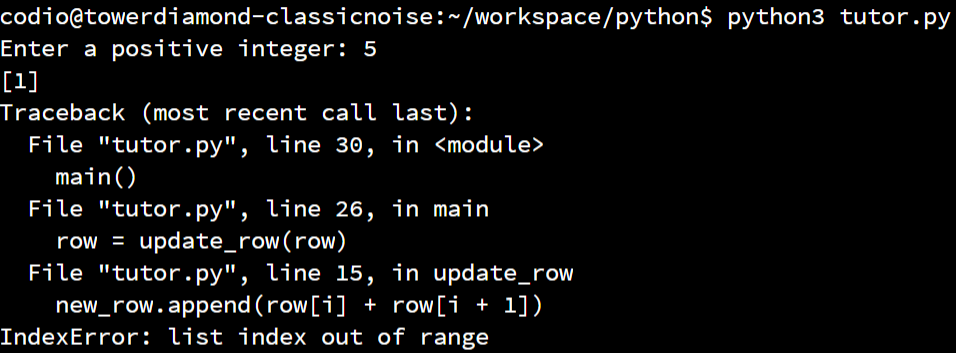
Uh oh! We’ve run into an error! This error is telling us that somewhere we are trying to access an index inside of a list that doesn’t exist. Helpfully, it tells us that we are doing this in the update_row() function, right inside of the for loop:
def update_row(row):
i = 0
new_row = [1]
while i < len(row):
new_row.append(row[i] + row[i + 1])
i = i + 1
new_row.append(1)
return new_rowSo, let’s see if we can figure out what is going on here. Let’s assume that it is failing when we are passing in the first row, which is simply the list [1]. On that line of code, we are appending a new item to the end of our new_list that is the sum of row[i] and row[i+1].
Ah ha! At this point, our row only contains a single item, so even if i is initially set to $0$, we cannot access an element that has index $1$ in that list. That’s where our logic error is coming from!
Since we need to access elements that are at one index higher than i, we must adjust our while loop so that it stops at the element before the last one. We can easily do that by modifying our while loop’s Boolean expression to i < len(row) - 1. If we make that change and try our program again, we should see the correct output:
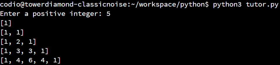
The full, working example code is shown here:
def positive_input():
x = int(input("Enter a positive integer: "))
while x <= 0:
print("Invalid input!")
x = int(input("Enter a positive integer: "))
return x
def update_row(row):
i = 0
new_row = [1]
while i < len(row) - 1:
new_row.append(row[i] + row[i + 1])
i = i + 1
new_row.append(1)
return new_row
def main():
n = positive_input()
row = [1]
print(row)
for i in range(1, n):
row = update_row(row)
print(row)
main()There we go! We’ve written a complete program that will generate Pascal’s Triangle for any given number of rows. It uses both while and for loops and lists to accomplish that goal. Try to work through this entire example and run the program many times along the way to make sure you have a good understanding of why it works before continuing in this lab.
You might be wondering why we’ve chosen to keep the logic error in this example program instead of simply fixing it in our explanation. As it turns out, that logic error was actually made by the author while writing this example, and we felt that it was best to demonstrate how to quickly identify and resolve such an error instead of simply explaining it away. Hopefully seeing how easy it is to make simple logic errors like this will help you understand that it can happen to anyone, and it is not a big deal to have to fix small bugs along the way.
In this lab, we introduced several major important topics in Python. Let’s quickly review them.
Lists in Python allow us to store multiple elements in a single variable, with each element identified by a unique index within the list.
Lists can be created using square brackets []:
list_a = []
list_b = [5, 3, 7]New elements can be added to a list using the append() method:
list_a = []
list_a.append(4)Items in a list can be accessed and updated using square brackets:
list_b = [5, 3, 7]
list_b[2] = list_b[0] + list_b[1]Lists can be iterated using both for loops and while loops:
list_b = [5, 3, 7]
for i in list_b:
print(i)
j = 0
while j < len(list_b)
print(list_b[j])
j = j + 1Lists should not be changed while iterating using a for loop.
When calling a function that accepts a list as a parameter, the argument is passed using call by reference instead of call by value. The original list can be modified by the function, but it cannot be replaced with a new list unless the reference to that new list is returned from the function.
Strings can be iterated just like a list, and we can use square brackets to access individual characters in a string. However, lists are still passed as call by value when provided as an argument to a function.
We can create a slice of a list by specifying a start, end and step value separated by colons. The values may be omitted, and may also be negative.
list_b = [5, 3, 7]
print(list_b[-1])
print(list_b[0:1])
print(list_b[0:2:2])
print(list_b[::-1])In theory, a dictionary is very similar to a list in Python - it is a data structure that can store many different items within a single variable. However, instead of just storing single values as elements and assigning them sequential indexes, dictionaries store a number of key-value pairs. A key is any value that can be used as a unique identifier for the associated value to be stored in the dictionary.
For example, we can use a dictionary to store the “score” for various words in the game of Scrabble
. In this case, our key would be the word stored as a string, such as "test", and the value would be an integer representing the score, 4. These two items make up a key-value pair ("test", 4) that can be stored in a dictionary.
There is one major rule that dictionaries must follow - each key in a dictionary must be unique. Or, put another way, if the dictionary already contains a value for a given key, and we try to add another value that uses the same key, the first value will be overwritten. So, we must be careful and make sure that the keys we choose to use are indeed unique so that they will work in a dictionary.
Dictionaries in Python can be created in much the same way as a list. We can create an empty dictionary using a set of curly braces {} as shown here:
dict_1 = {}We can also create a dictionary that contains some initial key-value pairs by placing them inside of the curly braces. Each key-value pair is separated by a comma , with the key provided first, followed by a colon : and then the value. Here’s a brief example:
dict_2 = {"a": 1, "b": 2, "c": 3}In this dictionary, the keys are the strings "a", "b", "c", and each one is associated with the values 1, 2, and 3, respectively.
Finally, to make it a bit easier to read our code, we can also reformat the code to create a dictionary across multiple lines, with each key-value pair shown on its own line as seen in this example:
dict_3 = {
"cat": "mammal",
"lizard": "reptile",
"goldfish": "fish",
"chickadee": "bird"
}This dictionary associates various animal species with the common name of their classification within the animal kingdom.
We can also easily add new items to a dictionary by simply providing a key inside of square brackets [] and then using an assignment statement to assign that key a value. Consider this example:
dict_1 = {}
dict_1["Kansas"] = "Topeka"
dict_1["Nebraska"] = "Lincoln"
dict_1["Missouri"] = "Jefferson City"Here, we start by creating an empty dictionary, and then we can add key-value pairs using the names of states as the key and the state’s capital city as the value.
Notice that we use square brackets [] to access individual items in a dictionary, just like with lists, but we use curly braces {} to create a dictionary. This can cause confusion for many new Python programmers. So, pay special attention to the syntax of each data structure, and remember that it can sometimes be difficult to tell whether a data structure in Python is a list or a dictionary without reading the code to see where it was created.
Once a dictionary contains items, we can access the value associated with a given key by providing that key within square brackets [] after the variable storing the dictionary. Here’s an example of what that looks like in Python:
dict_3 = {
"cat": "mammal",
"lizard": "reptile",
"goldfish": "fish",
"chickadee": "bird"
}
print(dict_3["cat"]) # mammalAs we can see, we’re able to provide the key "cat" and then access the associated value "mammal" that was stored in the dictionary.
What if we try to access a key that doesn’t exist? In that case, Python will raise a “KeyError” and the program will crash. So, we’ll have to be careful and make sure we only try to access keys that are actually stored in the dictionary, unless we are using them in an assignment statement to add a new key-value pair.
We can also update the value associated with a given key in a dictionary using an assignment statement, as shown here:
dict_3 = {
"cat": "mammal",
"lizard": "reptile",
"goldfish": "fish",
"chickadee": "bird"
}
dict_3["cat"] = "feline"
print(dict_3["cat"]) # felineIn this example, we are simply replacing the value for the key "cat" with a new string “feline”. Remember that the keys in a dictionary must be unique, so if we try to add a new value using the same key, it will simply overwrite the existing value associated with that key.
To really understand how dictionaries work in Python, let’s go through a quick example using Python Tutor. Consider the following Python program:
def main():
base = int(input("Enter a whole number: "))
powers = {}
for i in range(6):
powers["{}^{}".format(base, i)] = base ** i
print(powers)
main()This program will ask the user to provide a number as input, and then it will populate a dictionary where the key is a string representing a mathematical expression including that number, and the value will be the result of that expression. Let’s trace through this program in Python Tutor. As always, you can copy and paste the code in the tutor.py file in Codio, or click this Python Tutor
link to open it on the web.
When we start tracing the program in Python Tutor, we can skip ahead until it reaches the first line of code in the main() function, at which point we’ll see this state:
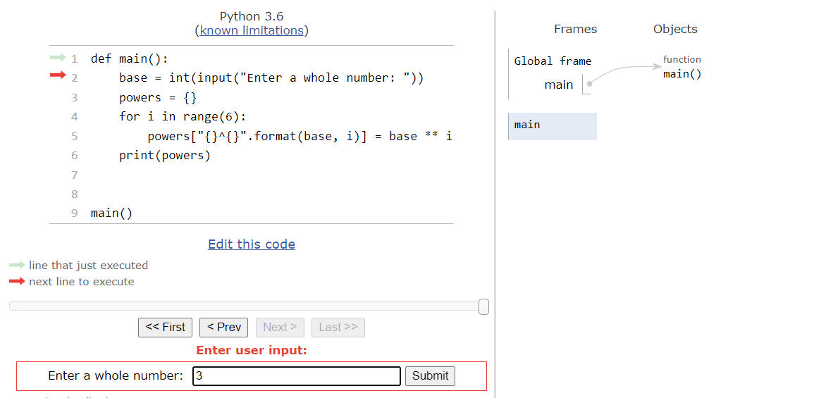
This first line of code asks the user to input a value. For this example, let’s assume the user inputs the string "3". So, we’ll store the integer value $3$ in the base variable as seen here:
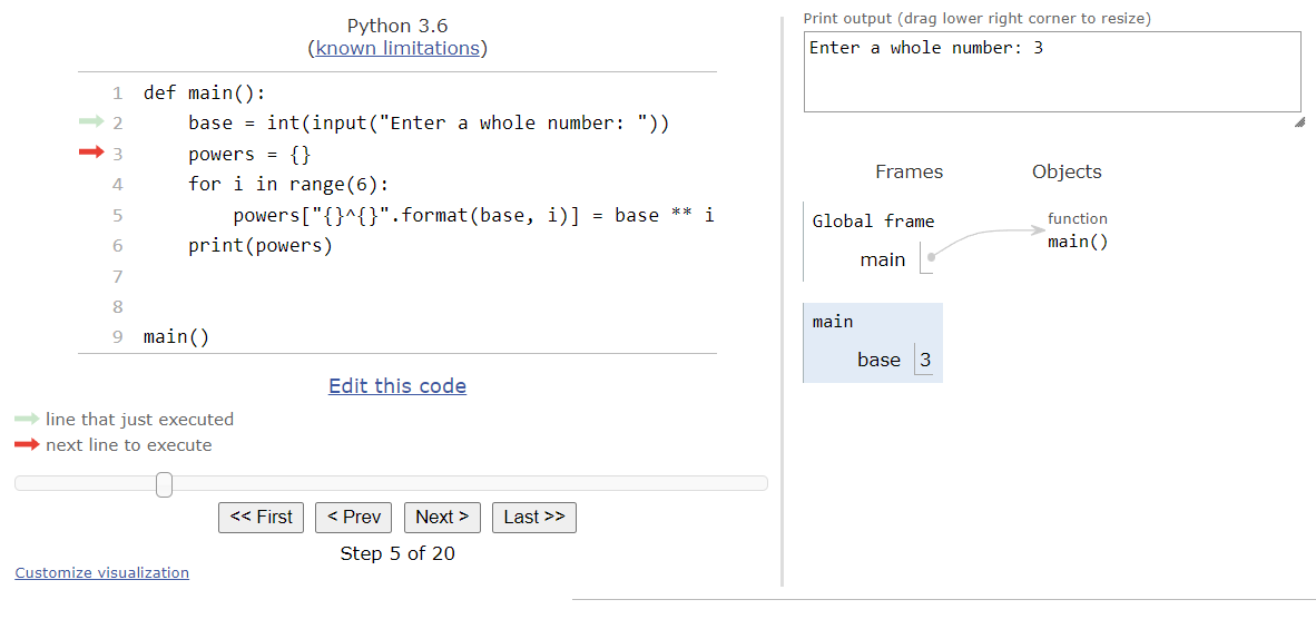
This line will create an empty dictionary in the powers variable. Just like lists in Python, a dictionary is actually stored in the objects area in memory, and the variable is simply a pointer, or reference, to the location in memory where the dictionary will be stored. So, after we execute that line of code, we should see this state:
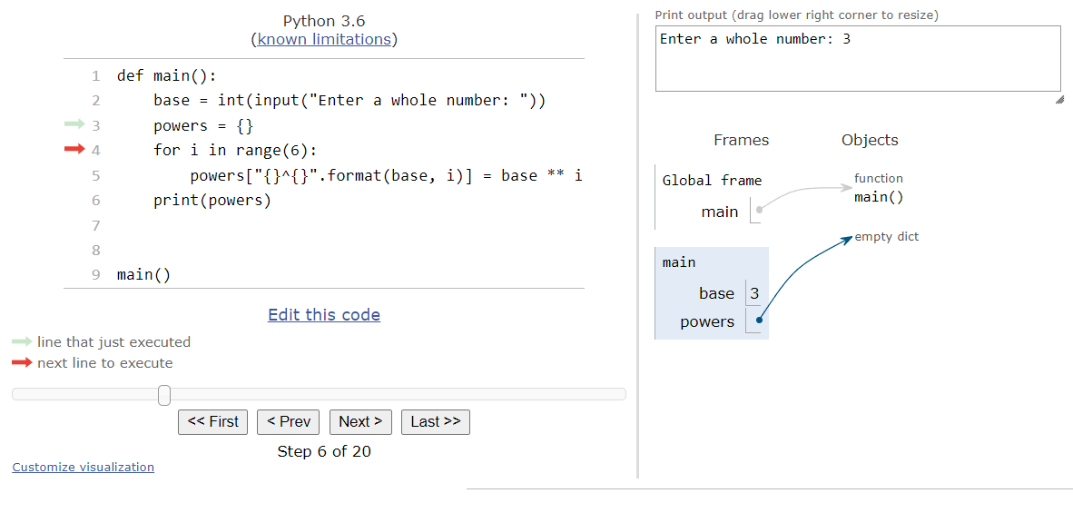
At this point, we reach the for loop. This loop will iterate $6$ times, so we’ll start by storing the first value $0$ in the iterator variable i and then entering the loop:
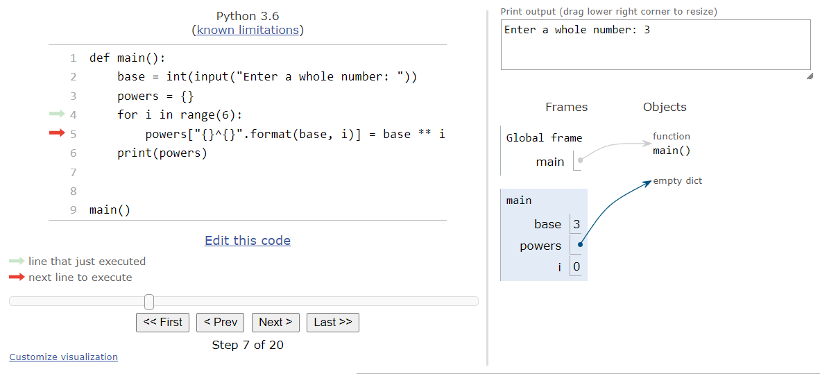
Inside of the loop, we see a single line of code that is pretty complex. This line will actually perform three different operations! First, it will generate a string using the string format() method, which will become the new key that is added to the dictionary. Then, it will compute the value of the base variable raised to the power of i. Finally, it will store that computed value in the dictionary associated with the newly created key. Once all of those steps are complete, we’ll see a new item in the dictionary as shown here:
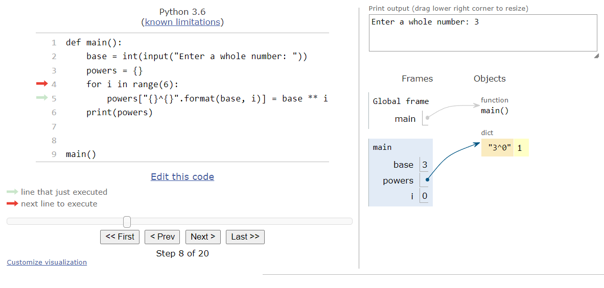
In Python Tutor, we can see the key for the item on the left, and then the associated value on the right. So, it is similar to how a list is represented, but instead of just showing the index, it will show the key and the value.
At this point, our program will loop back to the start of the for loop. Since there are more iterations to complete, we’ll update the iterator variable i to $1$, and then enter the loop again.

Once inside the loop, we’ll add another item to the dictionary, and then loop back to the top.
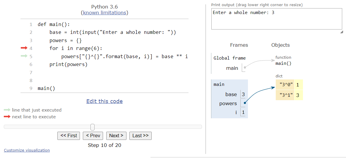
From here, hopefully it is clear what the rest of the program will do. Each time we enter the loop, we’ll generate a new key and value pair to add to the dictionary. So, let’s skip ahead to the end of the loop.
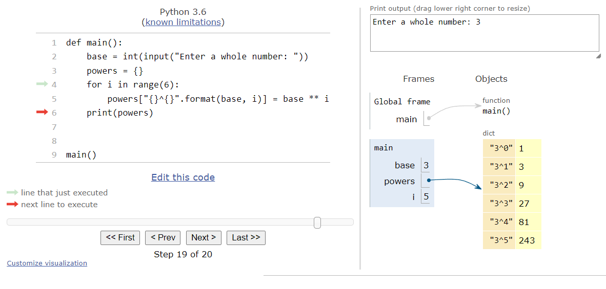
At the end of the program, we’ll print the contents of the dictionary to the terminal. Just like with lists, Python will print dictionaries in a clean and easy to understand format, as shown in the output in Python Tutor:
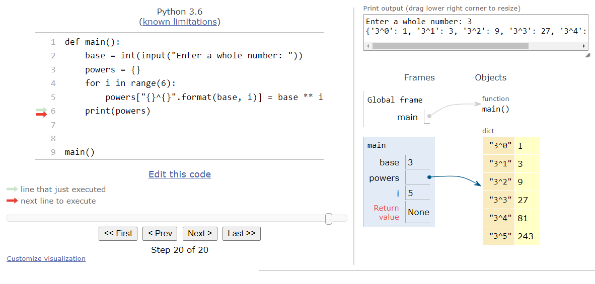
A full animation of this program is included below.
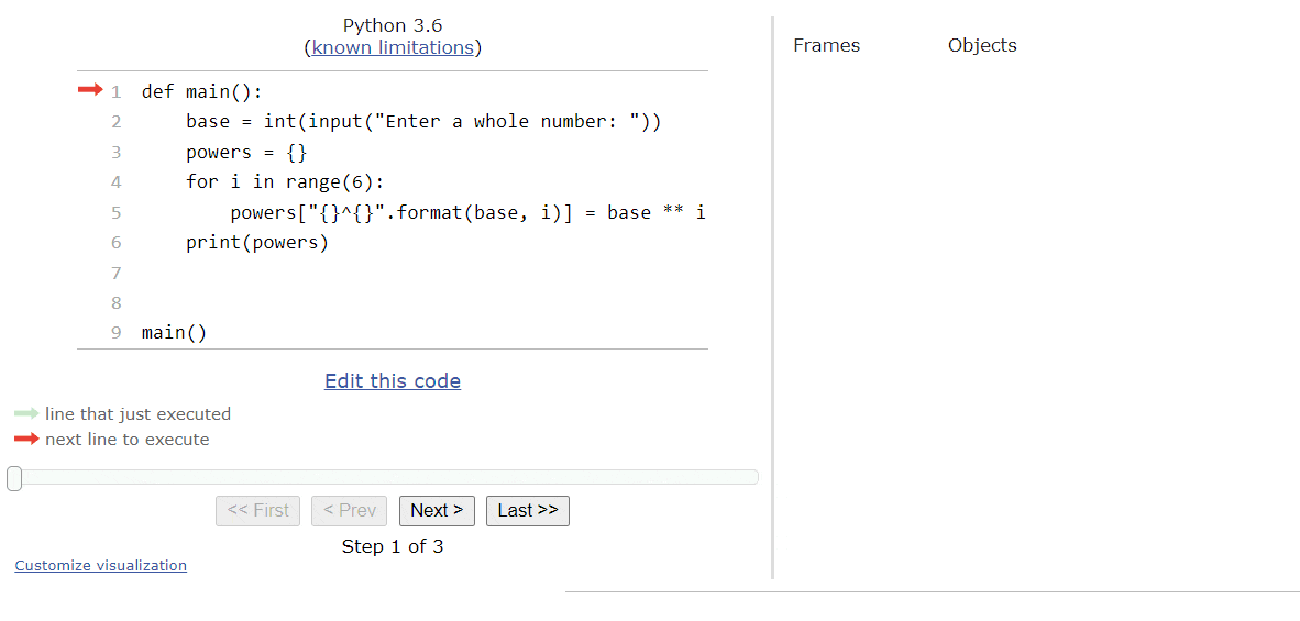
As we can see, dictionaries in Python work very similar to lists. When we create a dictionary, it is stored in the objects area in memory, and we can easily add, access, and even print the contents of a dictionary in our code. Dictionaries are really one of the most flexible data structures available in Python.
Another useful way we can work with dictionaries in Python is by iterating through them. In Python 3.6 and beyond, the items in a dictionary will be presented in the same order that they were added to the dictionary. This isn’t always the case in other languages or older versions of Python
There are two ways we can iterate through a dictionary in Python. Below is an example of the first, and simplest, method:
dict_3 = {
"cat": "mammal",
"lizard": "reptile",
"goldfish": "fish",
"chickadee": "bird"
}
for key in dict_3:
print("{}: {}".format(key, dict_3[key]))In this method, we are iterating through the entire dictionary using a for loop. However, the dictionary will only store the key for each key-value pair in the iterator variable. So, to access the value associated with the key, we can simply place it in square brackets after the dictionary’s variable name.
When we run this program, we should see the following output:
As we can see, it will print each key-value pair in the dictionary, one per line.
The other method we can use when looping through a dictionary allows us to access both the keys and values directly within the loop. Here’s an example of using that method:
dict_3 = {
"cat": "mammal",
"lizard": "reptile",
"goldfish": "fish",
"chickadee": "bird"
}
for key, value in dict_3.items():
print("{}: {}".format(key, value))In this method, instead of iterating through the dictionary itself, we iterate through the items() in the dictionary. When we call the items() function in a dictionary, we are given a list of the key-value pairs that it contains, and each key-value pair is stored as a tuple. From there, we can access each of the elements in the tuple individually using a comma , between two variable names. It is a bit complex, and touches on a few concepts in Python that we won’t cover in this course, but hopefully it makes sense by looking at the code.
When we run this program, we’ll receive the same output as the previous example:
While iterating through dictionaries is not as common as iterating through lists, it is still very important to know that it can be done. Hopefully you’ll find this example useful as you continue to work with dictionaries in Python.
Finally, let’s briefly look at how dictionaries operate when used as parameters to functions in Python. As we can probably guess from the earlier example in Python Tutor, dictionaries also use call by reference, just like lists.
Here’s a short example program in Python that demonstrates the use of dictionaries with functions.
def add_score(scores):
name = input("Enter a name: ")
score = int(input("Enter a score: "))
scores[name] = score
def average_score(scores):
total = 0
for key, value in scores.items():
total = total + value
return total / len(scores)
def main():
scores = {}
for i in range(4):
add_score(scores)
print(average_score(scores))
main()Let’s take a look at this program using Python Tutor to see how it works. As always, you can copy and paste this code into the tutor.py file on Codio, or click this Python Tutor
link in the lab to open it in a web browser.
First, Python Tutor will iterate through the code and record all of the functions in the objects area. Once it reaches the call to the main() function at the bottom, it will jump to the code inside of that function. At that point, we should see this state:
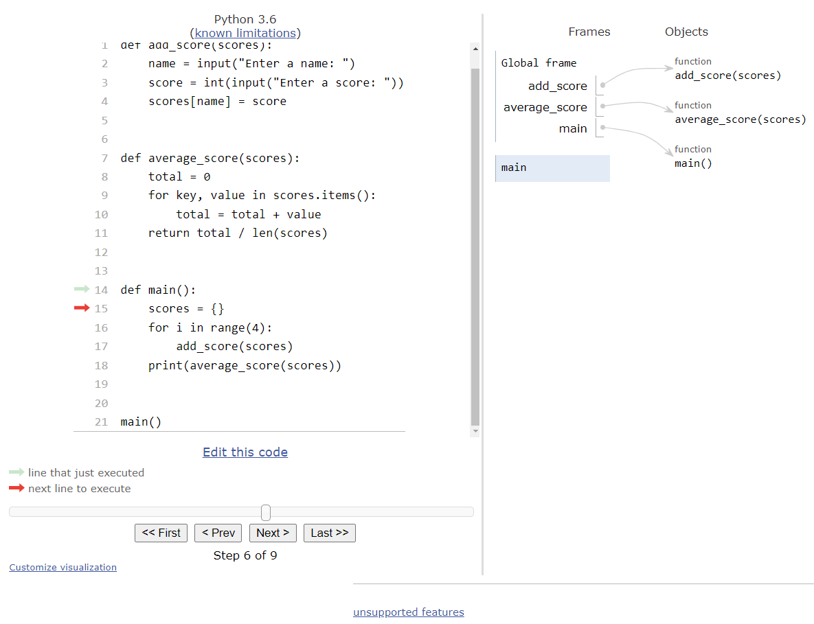
The first thing that this program will do is create an empty dictionary in the scores variable. So, after executing that line of code, we’ll see a new dictionary in the objects area in memory as shown here:
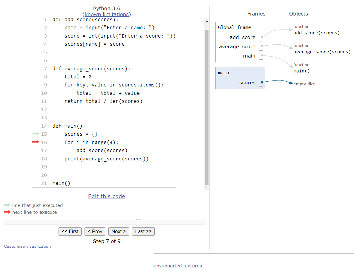
Next, we’ll reach a simple for loop that will iterate $4$ times, so we’ll enter that loop:
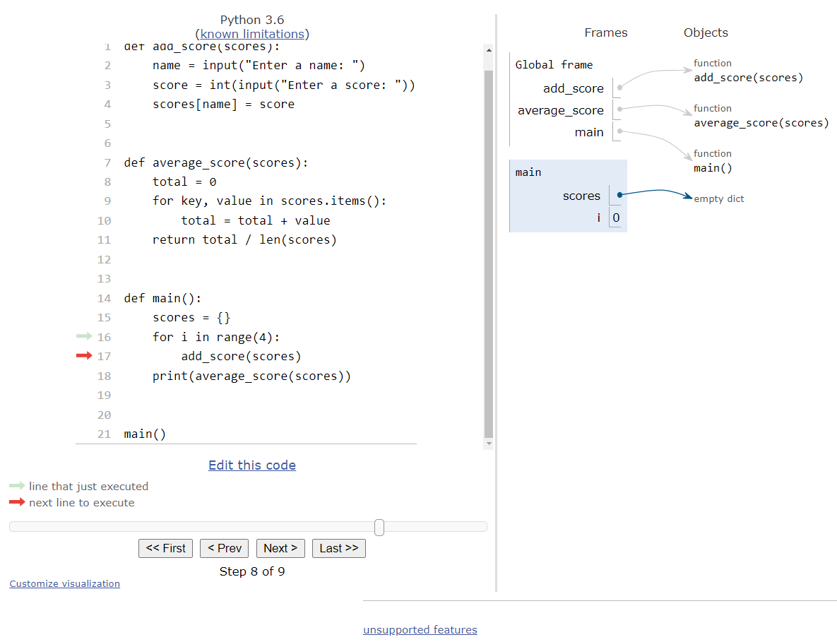
Inside of the loop, we are calling the add_score() function and providing the scores dictionary as an argument. So, when Python Tutor jumps to execute that function’s code, we’ll see it create a new frame for the function and populate that frame with the arguments provided as part of the function call:
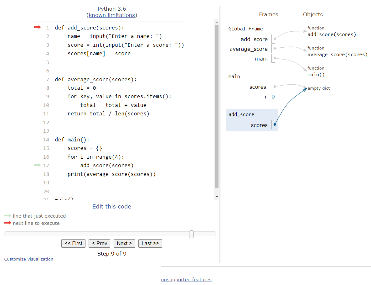
Since dictionaries in Python also use call by reference, we’ll see that the scores parameter in the add_score() function’s frame is just a reference back to the same empty dictionary that was created earlier. The scores variable in the main() function’s frame also points to the same object in memory.
The add_scores() function will prompt the user to input a name and a score. So, if we assume that the user inputs the string "Name" as the name, and "95" as the score, we should see this state in Python Tutor:
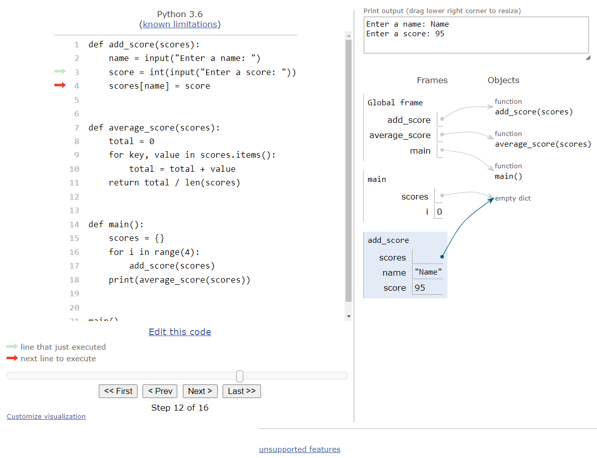
The last line of the function will add a new key-value pair to the dictionary, with the name used as the key and the score as the value. So, when the function is ready to return, we should see this state:
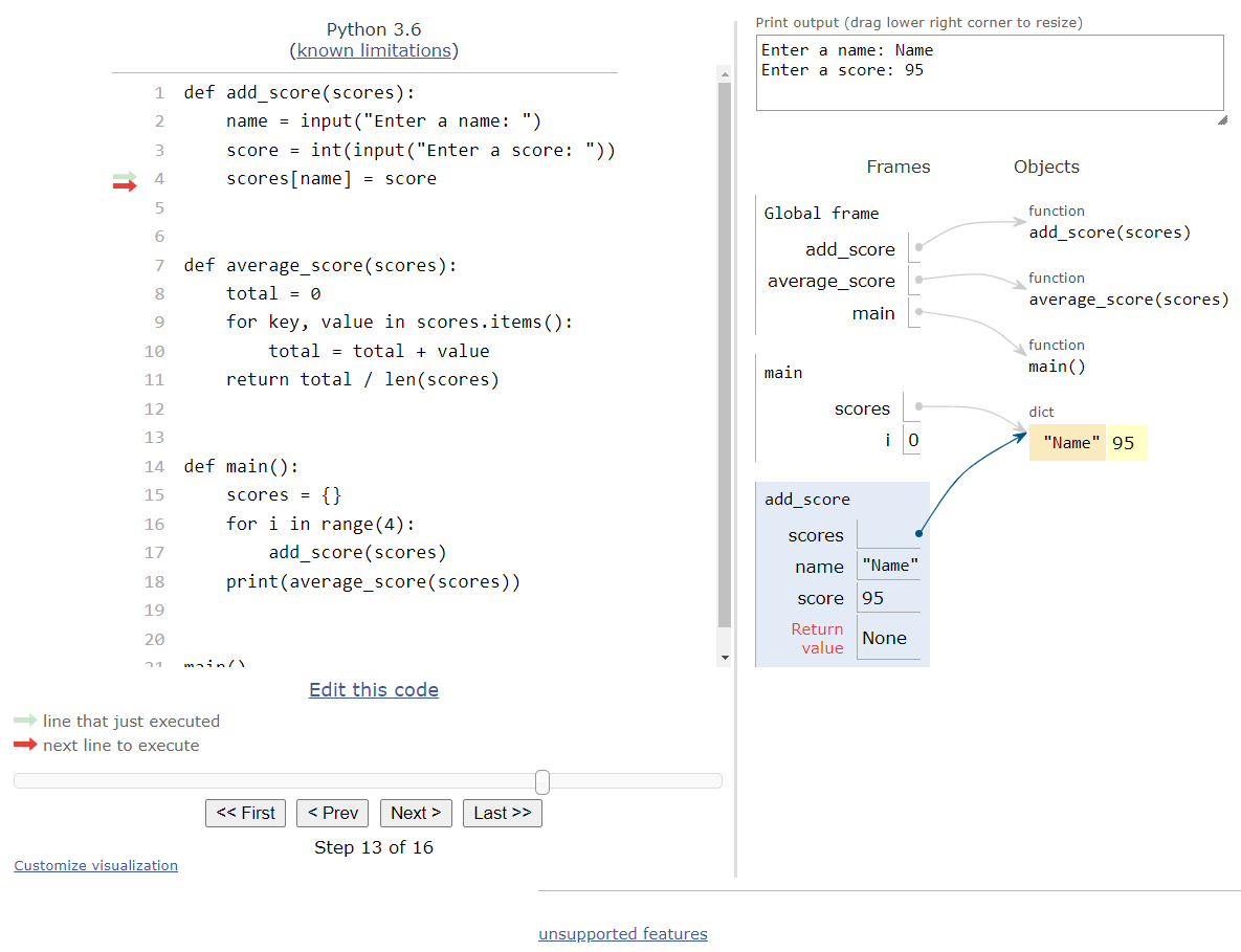
At this point, the control flow will return back to the main function, so our frame for the add_score() function will be removed. Thankfully, we can see that the new item we added to the dictionary is present in the one dictionary object in memory, which is also referenced from the main() function’s frame. So, once we are back in the main() function, we’ll see this state:
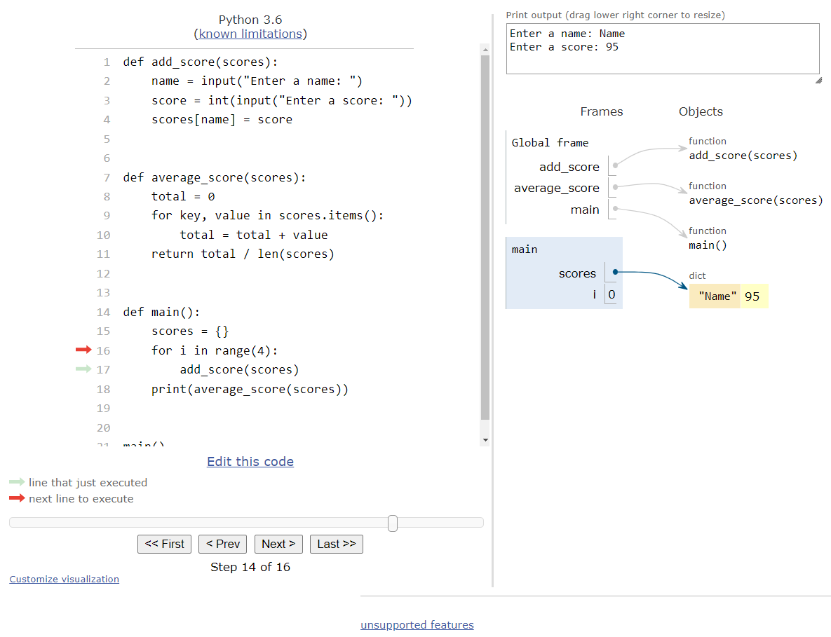
As we can see, dictionaries properly follow call by reference, so if we modify a dictionary that is passed to a function as an argument, we don’t have to return it back if we are just working with the same object.
At this point, the program will repeat that process three more times. We’ll skip ahead a bit to the end of the for loop in the main function, which will be this state:
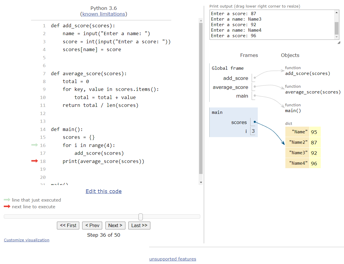
Here, our program will call the average_score() function to get the average of all of the scores in the dictionary. So, we’ll jump up to that function and provide the current dictionary as an argument, as shown here:
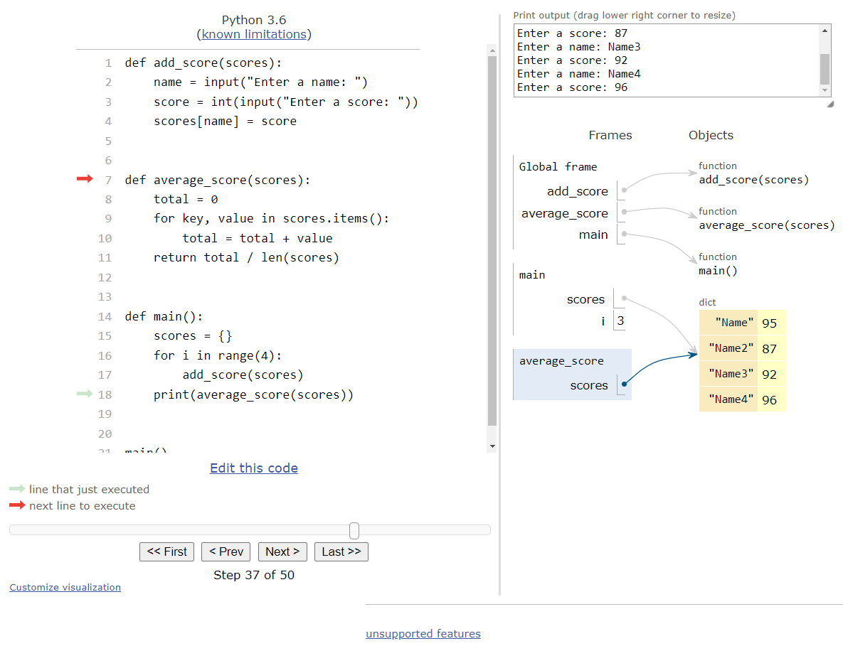
This function is very straightforward. However, let’s skip ahead a bit to when we are inside of the for loop, just to see what that looks like:
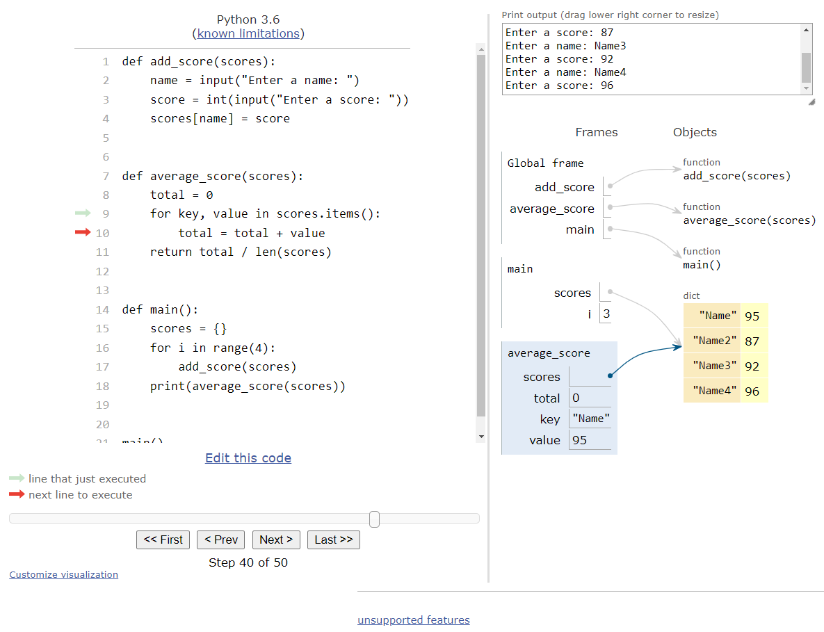
In our code, we are using the items() function of the dictionary to allow us to iterate over a list of the key-value pairs in the dictionary. So, inside of that for loop, we see both a key and a value variable, and they are populated with the first key and value from within our dictionary.
Once we’ve iterated through the entire dictionary, we’ll be at this state:
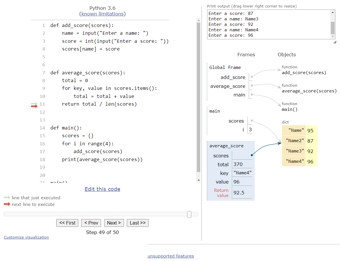
We’re ready to return from the function, and we’ve computed that our return value will be $92.5$, as seen the frame for the average_score() function. Once we are back in the main() function, we’ll simply print that value to the output:
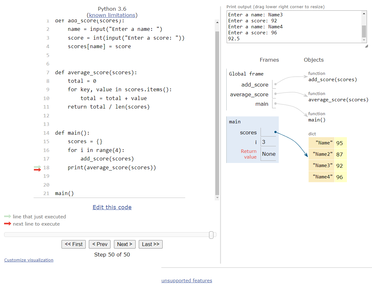
As we’ve seen in this example, working with dictionaries and functions in Python is practically identical to what we saw with lists - both data structures use call by reference when they are passed as arguments to a function. So, as long as we understand how Python is storing the data in memory, we can effectively build programs that operate the way we expect them to.
Finally, let’s go through a complete worked example program that uses dictionaries in Python. Consider the following problem statement:
Write a program that will compute the score of a given word in a game of Scrabble . Assume that there are no special squares present. The program should prompt the user to input a string that only contains letters, and then compute the total score of that string by summing the value assigned to each letter. If the user inputs a string that contains invalid characters, the program should prompt for additional input until a valid word is received.
This is a pretty simple program that can easily make use of a dictionary in Python. So, let’s go through the process of solving it!
As always, we can start our solution by including a main() function and a call to the main() function at the bottom of our code, as shown here:
def main():
main()Next, we’ll probably want to create a function to handle requesting input from the user. So, we’ll add that function to our solution as well, and we’ll call it from within the main() function itself:
def get_input():
def main():
word = get_input()
main()In the get_input() function, we’ll need the while loop structure we’ve already learned to handle input and verify that it is correct, so let’s go ahead and add that:
def get_input():
word = input("Enter a single word: ")
while # word is not valid
print("Error! Invalid Input!")
word = input("Enter a single word: ")
return word
def main():
word = get_input()
main()The only part we have to figure out is how we can determine if a word contains only valid characters. There are many different approaches we could follow, but the simplest is to use the isalpha() function that is part of the Python string data type. This function, along with many others, are described in the Official Python Documentation
.
So, let’s update our code to use that function as the Boolean expression in our while loop:
def get_input():
word = input("Enter a single word: ")
while not word.isalpha():
print("Error! Invalid Input!")
word = input("Enter a single word: ")
return word
def main():
word = get_input()
main()There we go! that covers the get_input() function, which will prompt the user to input a string that only contains letters.
Next, let’s look at writing a function that will accept a single word as a parameter, and then compute the score of that word according to the official Scrabble scoring rules.
We can start with a simple function definition as shown here:
def compute_score(word):First, let’s quickly convert the word we are given to lowercase, just in case the user has included any uppercase letters. Remember, we already know that this word should only contain letters, but it may be a mix of uppercase and lowercase. We can use the lower() function to make this conversion:
def compute_score(word):
word = word.lower()Next, we’ll need to iterate through each letter in the word. Since we can treat a string just like a list, we can use a for loop for this:
def compute_score(word):
word = word.lower()
for letter in word:We’ll also need some way to keep track of the total score, and then return that value at the end of the function. This is a pretty common pattern in programming known as the accumulator pattern. So, let’s add a total variable to our program, starting it at $0$ and then returning it at the end:
def compute_score(word):
word = word.lower()
total = 0
for letter in word:
# add letter's score to total
return totalFinally, we just need some way to convert a letter into a score in Scrabble. Thankfully, we can refer to the Official Scrabble FAQ to find out how many points each letter is worth:
There are many different ways we could build this program, but one simple way would be to assign each letter a value in a dictionary! To make things even easier, we can leave out all of the letters that are worth 1 point, and just include the letters with higher point values. By doing so, if we don’t find our desired letter in the dictionary, we can simply assume that the score must be 1!
So, let’s add that dictionary to our code:
def compute_score(word):
scores = {"d": 2, "g": 2, "b": 3, "c": 3, "m": 3, "p": 3,
"f": 4, "h": 4, "v": 4, "w": 4, "y": 4, "k": 5,
"j": 8, "x": 8, "q": 10, "z": 10}
word = word.lower()
total = 0
for letter in word:
# add letter's score to total
return totalNow that we have this dictionary available in our code, we can use it inside of the for loop to compute the total score of the word by looking up the value of each letter. However, before we can directly access a letter, we first must determine if a given letter is contained in the dictionary. In Python, we can do this using the in keyword. So, we can add an if statement inside of our for loop that is structured as shown here:
def compute_score(word):
scores = {"d": 2, "g": 2, "b": 3, "c": 3, "m": 3, "p": 3,
"f": 4, "h": 4, "v": 4, "w": 4, "y": 4, "k": 5,
"j": 8, "x": 8, "q": 10, "z": 10}
word = word.lower()
total = 0
for letter in word:
if letter in scores:
total = total + scores[letter]
else:
total = total + 1
return totalThe Boolean expression letter in scores will return true if the current letter in our word is present as a key in the dictionary scores. The same syntax also works for determining if an element is present in a list!
We can complete our program by simply printing the score returned by the compute_score() function in our main() function. So, the complete program is shown below:
def get_input():
word = input("Enter a single word: ")
while not word.isalpha():
print("Error! Invalid Input!")
word = input("Enter a single word: ")
return word
def compute_score(word):
scores = {"d": 2, "g": 2, "b": 3, "c": 3, "m": 3, "p": 3,
"f": 4, "h": 4, "v": 4, "w": 4, "y": 4, "k": 5,
"j": 8, "x": 8, "q": 10, "z": 10}
word = word.lower()
total = 0
for letter in word:
if letter in scores:
total = total + scores[letter]
else:
total = total + 1
return total
def main():
word = get_input()
print(compute_score(word))
main()We can confirm our program works correctly by running it and testing a few different inputs, as shown below:
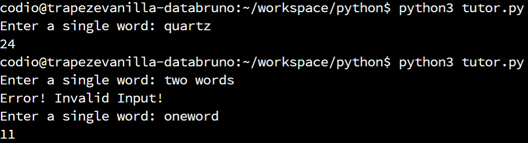
This example shows a great way to use dictionaries in our program - we can assign values to various keys, and then easily look them up in the dictionary as needed. Feel free to run this example in Python Tutor on your own to see how it works, and see if you can come up with your own high-scoring Scrabble words.
In this lab, we introduced several major important topics in Python. Let’s quickly review them.
Dictionaries in Python allow us to store key-value pairs in a single data structure. Keys are used to uniquely identify an associated value.
Dictionaries can be created using curly brackets {}:
dict_1 = {}
dict_2 = {"a": 1, "b": 2, "c": 3}New elements can be added to a dictionary by providing a new key in square brackets:
dict_2 = {"a": 1, "b": 2, "c": 3}
dict_2["d"] = 4Items can also be accessed and updated using square brackets
dict_2 = {"a": 1, "b": 2, "c": 3}
dict_2["c"] = dict_2["a"] + dict_2["b"]Dictionaries can be iterated by just the keys or by the keys and values in a tuple:
dict_3 = {
"cat": "mammal",
"lizard": "reptile",
"goldfish": "fish",
"chickadee": "bird"
}
# keys only
for key in dict_3:
print("{}: {}".format(key, dict_3[key]))
# keys and values
for key, value in dict_3.items():
print("{}: {}".format(key, value))When calling a function that accepts a dictionary as a parameter, the argument is passed using call by reference instead of call by value. The original dictionary can be modified by the function, but it cannot be replaced with a new dictionary unless the reference to that new dictionary is returned from the function.
