CC 410 - Advanced Programming

This is the textbook for CC 410 - Advanced Programming.

Course Description: Advanced programming techniques and projects. Concepts from simulation and modeling, media applications, secure design, information management, parallelism, and networking. Software development methodologies, processes, and design patterns. Practical experience with professional communication and collaboration.

Prerequisites: CC 315

Credits: 4

Subsections of CC 410 - Advanced Programming

Chapter 0

Introduction

Welcome to CC 410!

Subsections of Introduction

Course Introduction

YouTube Video

Resources

Video Script

Hello and welcome to the Computational Core program!

My name is Russ Feldhausen, and I’ll be one of the instructors for this program. My contact information is shown here, and is also listed on the syllabus

[Slide 2]

There are many other instructors and TAs for this program that you may interact with or see in the tutorial videos. They all have been instrumental in the development of this program. Specifically, I’d like to recognize the work of Nathan Bean, the developer of the CIS 400 course on which this course is based.

[Slide 3]

In this course we will primarily use a KSU email group (cc410-help or cc410-help@ksuemailprod.onmicrosoft.com ) to communicate. Email sent to this address is forwarded to all instructors and TAs. Our replies to you will also be shared amongst the instructors and TAs so we all have access to the assistance you have already received. We will respond to you within a business day, so be aware that a question emailed Friday night may not receive an answer before Monday. Please read and adhere to the guidance on Netiquette in the syllabus for all electronic communications.

[Slide 3]

In addition to email and Canvas, we’ll be using the online learning platform Codio for most of the programming tutorials and projects in this program. We’ll also discuss how to use Codio later in this module.

[Slide 5]

The Computational Core program consists of several courses, and each course contains a number of learning modules. In general, there are about 12-15 modules per course. Each module will usually consist of an interactive tutorial using Codio, followed by a quiz through Canvas, and lastly a programming project in Codio. In CC 410, there will also be several guided examples for you to follow and submit. The modules themselves are gated, which means that you much complete each item in the module before continuing. In addition, the modules enforce prerequisite requirements from other modules. For CC 410 you must complete them in order starting with module 0.

You are welcome to work on this course at any time during the week as your schedule allows, provided that you complete each module before the listed due date. There will be roughly one module due each week. Unlike other Computational Core courses, CC 410 does not include many auto-graded assignments. This is primarily due to the open-ended nature of the course. Instead, your code will be reviewed by an instructor or TA and you’ll receive feedback through Canvas and Codio. In some instances, you may be encouraged to redo parts of an assignment for additional credit. We will strive to provide feedback on an assignment within one week of it being submitted.

[Slide 6]

Looking ahead to the rest of this introductory module, you’ll see that there are a few more items to be completed before you can move on. In the next video, I’ll discuss a bit more information about navigating through this course on Canvas and using the Codio learning environment.

[Slide 7]

One thing I highly encourage each of you to do is read the syllabus for this course in its entirety, and let us know if you have any questions. My view is that the syllabus is a contract between me as your teacher and you as a student, defining how each of us should treat each other and what we should expect from each other. We have made a few changes to the standard syllabus template for this program, and those changes are clearly highlighted. Finally, the syllabus itself is subject to change as needed as we adapt this program to meet the needs of its students, and all changes will be clearly communicated to everyone before they take effect.

[Slide 8]

One very important part of the syllabus that every student should read is the late work policy. First off, each module has a due date, and you may work on that module at any time before it is due, provided you have met the prerequisites. As discussed before, you must do all the readings and assignments in a module, preferably in listed order, before moving on, so you cannot jump ahead. A module is considered completed when all items have been completed.

[Slide 9]

For the purposes of grading, we will use the date and time that the confirmation quiz was submitted at the end of each module to determine when the module was completed. This is due to the way that Codio handles grading, as it may resubmit previously graded assignments if an error in the module is corrected, making a previously completed assignment appear to be submitted late.

If a module is completed after the due date, a penalty of 10% of the total points of each assignment will be deducted for each day the assignment is late. Therefore, if an assignment is submitted 3 days late, it will be subject to a 30% penalty of the total number of points possible on that assignment. After 10 days, no points will be awarded for a late submission.

However, even if a module is late, it still must be completed before you can move on to a later module. So, it is very important to avoid getting behind in this course, as it can be very difficult to get back on track. If you ever find that you are struggling to keep up, please don’t be afraid to contact either the instructors or GTAs for assistance. We’d be happy to help you get caught back up quickly.

The grading in this course is very simple. First, 10% of your final grade will depend on the grades you receive from each of the tutorials and quizzes throughout the course. Next, 10% of your grade will come from the interactive examples that precede several projects. The next 40% of your grade will come from the numerous project milestones throughout the course, of which there will be approximately 10. There will also be a couple of “concept quizzes” throughout the semester, which are a bit longer than a normal quiz and will ask you to apply what you’ve learned to a novel situation. Those are worth 15% of your grade. Finally, the last 25% of your grade will come from the final project in the course, which will be discussed in a later video. In this program, the standard “90-80-70-60” grading scale will apply, though I reserve the right to curve grades up to a higher grade level at my discretion. Therefore, you will never be required to get higher than 90% for an A, but you may get an A if you score slightly below 90% if I choose to curve the grades.

[Slide 10]

This is intended to be a completely online, self-paced course. There are no mandatory scheduled course times. All of the content is available online, so you can work whenever and wherever you want. It could be a 3-hour block once a week, or a few minutes here and there between classes. It’s really up to you and your schedule. However, remember that each module may require 12 to 16 or more hours of work to complete, so make sure you have plenty of time available to devote to this course.

In addition, due to the flexible online format of this class, there won’t be any long lecture videos to watch. Instead, each module will consist of a guided tutorial and several short videos, each focused on a particular topic or task. Likewise, there won’t be any textbooks required, since all of the information will be presented in the interactive tutorials through Codio. Finally, since we are using Codio as our learning platform, you won’t have to deal with installing and using a clunky integrated development environment, or IDE, just to learn how to program. Codio helps make learning to program quick and painless by moving everything to the web.

[Slide 11]

What hasn’t changed, though, is the basic concept of a college course. You’ll still be expected to watch or read about 6-9 hours of content to complete each module. In addition to that, each project assignment may require another 6-9 hours of work to complete. If you plan on doing a module each week, that roughly equates to 6 hours of content and 6 hours of homework each week, which is the expected workload from a 3-4 credit hour college course.

From my experience, I can definitely share that the number one reason students struggle in this class is due to poor time management, not the complexity of the material. So, make sure you are planning to dedicate enough time to this course, and strive to start assignments as soon as you receive them so you have lots of time to get help if you get stuck.

[Slide 12]

For this course, the only supplies you’ll need as a student are access to a modern web browser and a broadband internet connection. No other special hardware or software is necessary! However, in this course you will also be able to do some development on your own computer using Visual Studio Code and Ubuntu. We’ll provide some short videos to help you get started if you choose to go that route, but it is not required. Due to the complex nature of this course, we do not recommend using phones, tablets, or Chromebooks if you choose to do development on your own systems.

[Slide 13]

Finally, as you are aware, this course is always subject to change. This is a relatively new program here at K-State, and we’re always working on new and interesting ideas to integrate into the courses. The best advice I have is to look upon this graphic with the words “Don’t Panic” written in large, friendly letters. If you find yourself falling behind, or not understanding seek our help via cc410-help.

[Slide 14]

So, to complete this module, there are a few other things that you’ll need to do. The next step is to watch the video on navigating Canvas and Codio, which will give you a good idea of how to most effectively work through the content in this course.

[Slide 15]

To get to that video, click the “Next” button at the bottom right of this page.

Subsections of Course Introduction

Navigating Canvas & Codio

YouTube Video

Resources

Video Script

This course makes extensive use of several features of Canvas which you may or may not have worked with before. To give you the best experience in this course, this video will briefly describe those features and the best way to access them.

When you first access the course on Canvas, you will be shown this homepage. It contains quick links to the course syllabus and Piazza discussion boards. This is handy if you just need to jump to a particular area.

Let’s walk through the options in the main menu to the left. The first section is Modules, which is where you’ll primarily interact with the course. You’ll notice that I’ve disabled several of the common menu items in this course, such as Files and Assignments. This is to simplify things for you as students, so you remember that all the course content is available in one place.

When you first arrive at the Modules section, you’ll see all of the content in the course laid out in order. If you like, you can minimize the modules you aren’t working on by clicking the arrow to the left of the module name. I’ll do so, leaving the introductory module open.

As you look at each module, you’ll see that it gives quite a bit of information about the course. At the top of each module is an item telling you what parts of the module you must complete to continue. In this case, it says “Complete All Items.” Likewise, the following modules may list a number of prerequisite modules, which you must complete before you can access it.

Within each module is a set of items, which must be completed in listed order. Under each item you’ll see information about what you must do in order to complete that item. For many of them, it will simply say view, which means you must view the item at least once to continue. Others may say contribute, submit, or give a minimum score required to continue. For assignments, it also helpfully gives the number of points available, and the due date.

Let’s click on the first item, Course Introduction, to get started. You’ve already been to this page by this point. Many course pages will consist of an embedded video, followed by links to any resources used or referenced in the video, including the slides and a downloadable version of the video. Finally, a rough video script will be posted on the page for your quick reference.

While I cannot force you to watch each video in its entirety, I highly recommend doing so. The script on the page may not accurately reflect all of the content in the video, nor can it show how to perform some tasks which are purely visual.

When you are ready to move to the next step in a module, click the Next button at the bottom of the page. Canvas will automatically add Next and Previous buttons to each piece of content which is accessed through the Modules section, which makes it very easy to work through the course content. I’ll click through a couple of items here.

At any point, you may click on the Modules link in the menu to the left to return to the Modules section of the site. You’ll notice that I’ve viewed the first few items in the first module, so I can access more items here. This is handy if you want to go back and review the content you’ve already seen, or if you leave and want to resume where you left off. Canvas will put green checkmarks to the right of items you’ve completed.

Continuing down the menu to the left, you’ll find the usual Canvas links to view your grades in the course, as well as a list of fellow students taking the course.

===

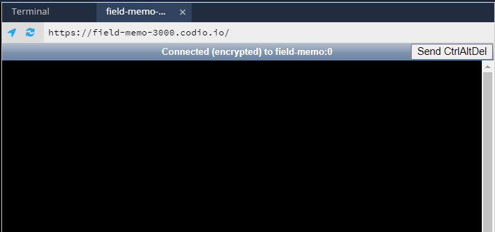
Now, let’s go back to Canvas and load up one of the Codio projects. To load the first Codio projects, click the Next button at the bottom of this page to go to the next part of this module, which is the Codio Introduction tutorial. On that page, there will be a button to click, which opens Codio in a new browser window or tab.

Once Codio loads, it should give you the option to start the Guide for that module. You’ll definitely want to select that option whenever you load a Codio project for the first time.

From there, you can follow the steps in that guide to learn more about the Codio interface. The first page of the guide continues this video. I’ll see you there!

Where to Find Help

YouTube Video

Resources

Video Script

As you work on the materials in this course, you may run into questions or problems and need assistance. This video reviews the various types of help available to you in this course.

First and foremost, anytime you have a questions or need assistance in the Computational Core program, please send an email to the appropriate help group for this course. In this case, it would be cc410-help, or cc410-help@ksuemailprod.onmicrosoft.com . That email goes to the instructors and GTAs, and is your best chance to get a quick response. We’ll respond to your email within one business day.

Beyond email, there are a few resources you should be aware of. First, if you have any issues working with K-State Canvas, K-State IT resources, or any other technology related to the delivery of the course, your first source of help is the K-State IT Helpdesk. They can easily be reached via email at helpdesk@ksu.edu . Beyond them, there are many online resources for using Canvas, all of which are linked in the resources section below the video. As a last resort, you may also want to email the help group, but in most cases we may simply redirect you to the K-State helpdesk for assistance.

Similarly, if you have any issues using the Codio platform, you are welcome to refer to their online documentation. Their support staff offers a quick and easy chat interface where you can ask questions and get feedback within a few minutes.

If you have issues with the technical content of the course, specifically related to completing the tutorials and projects, there are several resources available to you. First and foremost, make sure you consult the vast amount of material available in the course modules, including the links to resources. Usually, most answers you need can be found there.

If you are still stuck or unsure of where to go, the next best thing is to post your question as an email to the help group. As discussed earlier, the instructors and GTAs will do their best to help you as soon as they can.

Of course, as another step you can always exercise your information-gathering skills and use online search tools such as Google to answer your question. While you are not allowed to search online for direct solutions to assignments or projects, you are more than welcome to use Google to access programming resources such as StackOverflow, language documentation, and other tutorials. I can definitely assure you that programmers working in industry are often using Google and other online resources to solve problems, so there is no reason why you shouldn’t start building that skill now.

Next, we have grading and administrative issues. This could include problems or mistakes in the grade you received on a project, missing course resources, or any concerns you have regarding the course and the conduct of myself and your peers. Since this is an online course, you’ll be interacting with us on a variety of online platforms, and sometimes things happen that are inappropriate or offensive. There are lots of resources at K-State to help you with those situations. First and foremost, please email me directly as soon as possible and let me know about your concern, if it is appropriate for me to be involved. If not, or if you’d rather talk with someone other than me about your issue, I encourage you to contact either your academic advisor, the CS department staff, College of Engineering Student Services, or the K-State Office of Student Life. Finally, if you have any concerns that you feel should be reported to K-State, you can do so at https://www.k-state.edu/report/ . That site also has links to a large number of resources at K-State that you can use when you need help.

Finally, if you find any errors or omissions in the course content, or have suggestions for additional resources to include in the course, email the help group. There are some extra credit points available for helping to improve the course, so be on the lookout for anything that you feel could be changed or improved.

So, in summary, reviewing the existing course content should always be your first stop when you have a question or run into a problem, since most issues can be solved there. If you are still stuck, email cc410-help to ask for assistance, and we’ll get back to you within a business day. For issues with Canvas or Codio, you are also welcome to refer directly to the resources for those platforms. For grading questions and errors in the course content or any other issues, please email cc410-help or the instructors directly for assistance.

Our goal in this program is to make sure that you have the resources available to you to be successful. Please don’t be afraid to take advantage of them and ask questions whenever you want.

Subsections of Where to Find Help

How to Learn Programming

YouTube Video

Resources

Video Script

Before we launch into the course itself, I wanted to take a few minutes to share some information with you regarding what we know about how students learn to program. This isn’t just anecdotal evidence from computer science teachers like me, but theories and research from education researchers who study how humans learn new skills and abilities throughout their lives.If I had to summarize all of this information in as few words as possible, I’d simply say “do the work.” Learning to program is difficult, and the only way to really get good at it is through constant practice and learning. However, that greatly oversimplifies the information that I want to share, and I’m hoping that you’ll find some helpful takeaways from this video that you can incorporate into your learning process.

Before I begin, I want go give all the credit to Nathan Bean for developing this information as part of his CIS 400 course. He graciously allowed me to use his hard work here, and I encourage you to check out his original version, which is available at the URL shown on this slide.

The statement “do the work” is a shorter version of a very common quote from educators, which is “the person doing the work is the person doing the learning.” I couldn’t find a solid reference for who said it first, so I’ll just attributed it to various educators throughout time. This really highlights one of the biggest struggles many students run into when learning to program. There are so many guides online, and the answer to many simple problems can be found through a quick Google search. You can just copy and paste the code, and then your program works. However, did you really learn how to write that program and what it does, or just how to find a quick answer? While this may be a useful tactic from time to time, if you rely too much on other people to do your coding, you really won’t learn it yourself. This is just like learning to shoot free throws on a basketball court or beating your best time in a speedrun - you can’t just watch someone do it and expect to do it yourself (believe me, I’ve tried). So, if you aren’t doing the work, you aren’t really learning.

Next, let’s address a major myth in computer science. I’ve heard this many times: “some people are just natural born programmers, and others simply cannot learn to program.” And yes, on the surface, it may appear to be this way. Some students just seem to have a knack for programming, and you may sit and struggle and not really get anywhere. However, there is no innate skill or ability that makes you good at programming.

Instead, let’s reframe what it means to learn programming. At its core, programming is learning to write steps to solve problems in a way that a computer can perform those steps. That’s really what we are doing when we learn programming.

So, we must focus on learning how to write those steps with the proper exactitude and precision so that they make sense, and we must understand how a computer functions to be able to program that computer effectively. So, when you see someone who is good at programming, it’s not because they are good at some esoteric skill that you’ll never have - they just know how to express their steps properly and know enough about how a computer works to make their program do what they want. That’s really it! And, to be honest, after a single semester of learning to program, you’ll have all the skills you need to do both of those things! If you know how to make conditionals, loops, functions, and use simple variables and arrays, that’s really all you need. Everything else that comes after that is just refining those skills to make your programs more powerful and your coding more efficient.

So, how do we learn these skills? Well, there are a couple of important pieces we need to make sure are in the right place first. For starters, we need to have the correct mindset. Many times I’ll see students struggle to learn how to program, and they’ll say things like what you see on this slide. “Its too hard.” “I don’t understand this.” “I give up.” Statements like this are the sign of a “fixed mindset,” and they can be one of the greatest blockers preventing you from really learning to program. Just like learning any other skill, you have to be open to instruction and willing to learn, or else you’ve failed before you even started.

Instead, we want to focus on building a growth mindset. In the TED talk by Carol Dweck that is linked below this video, which I encourage you to watch, she talks about the power of “yet.” We can turn these statements around by simply adding positive power of “yet” - “I don’t understand this yet.” “I love a good challenge.” “I’ll keep trying until I get it.” Going into a programming project with a mindset that is open to growth and change is really an important first steps. When I feel like I’m getting a fixed mindset, I like to think about how difficult it would be to teach a child to tie their shoes if they don’t want to learn. As soon as I realize that, it is pretty easy to recognize that same problem in myself and work to correct it.

So, once we have our growth mindset, how do we actually learn to program? To understand that, let’s dive a bit into the world of educational theory and the work of Jean Piaget. Piaget was a biologist and psychologist who studied how young children acquired new knowledge, and he helped pioneer the concept of Constructivism, one of the most influential philosophies in education. You can read more about Constructivism in the links below this video.

One particular thing that Piaget worked on was a theory of genetic epistemology. Epistemology is the term for the study of human knowledge, so genetic epistemology is the study of the origins, or genesis, of that knowledge. Put more clearly, it’s the study of how humans create new knowledge. This concept was inspired by research done on snails - he was able to prove that two previously distinct species of snails were actually the same by moving snails from one habitat to another and observing how they modified their behaviors and how their shells grew to match the snails in the new habitat. Put clearly, the snails displayed an altered behavior based on their environment. They tried to exist in equilibrium with their environment by adapting their behaviors to fit what they now experienced in the word.

Piaget suspected that something similar happens when humans try to learn something - the brain tries to adapt itself to maintain an equilibrium in its environment, which in this case is the existing knowledge it contains. So, when the brain is exposed to new ideas, it must somehow adjust to account for that new information. Piaget proposed two different mechanisms for how this occurs: assimilation and accommodation. In assimilation, new knowledge can be added to existing structures in the brain. For example, if you are exposed to a new color, such as periwinkle, you can see that it falls somewhere between blue and violet, two colors you already know. So, you can assimilate that new knowledge into the existing knowledge without a major disruption to your mental structure of existing colors. Accommodation, on the other hand, happens when your brain must radically adapt to new information for which no existing structures exist. This can be very difficult, and can lead to a lot of struggle and frustration when trying to get “over the hump” on a new subject. Think about learning algebra or a new language for the first time - you really don’t have anything you can use to help understand this new material, so you just have to keep at it until those new structures are formed in your brain.

Unfortunately, to achieve accommodation, your brain simply has to build brand new structures to store and represent all of this new information, and that process is difficult and takes time. Put another way, it takes significant stimulus, usually in the form of doing homework, struggling with difficult problems and wrestling with the new information to try and understand it all, to create enough disequilibrium in your brain that, coupled with a growth mindset, will allow accommodation to occur. However, when all the pieces are in the right place, and you work hard and have a growth mindset, then…

EUREKA! The structures will form, and you’ll get over that huge hurdle, and things will start falling into place. It may not happen all at once, but it does happen (you’ve probably had it happen to you several times already - think about some eureka moments from your past - were they related to learning a new skill?). Of course, there’s a good chance that your brain might form a few incorrect structures in the process, so you’ll have to overcome those as you continue to learn. I still struggle to spell some words because my brain formed incorrect structures when I was still learning. But, if you continue to work hard and be open to learning, you’ll eventually sort those errors out as well.

Let’s look at one other concept in education, which is called stage theory. Piaget identified four stages that children go through as they learn to reason about the world. Those four stages are shown on this slide. In the sensorimotor stage, the child is just using their senses to interact with the world, without any real understanding of what will happen when they perform an action. This is best represented by babies and toddlers, who touch and taste everything in their surroundings. Next, the preoperational stage is represented in young children as they start to think symbolically about the world, using pictures and words to represent actions and objects. They then progress to the concrete operational stage, where they can begin to think logically and understand how concrete events happen. They can also start to think inductively, building the general principles of the world from their specific experiences. For example, if they observe that cooked spaghetti is better than raw spaghetti, they might reason that other foods like potatoes are better cooked than raw. Finally, the last stage is the formal operational stage. This stage is represented by the ability to work fully with an abstract work, formulating and testing hypotheses to truly understand how the world works and predict how new items will work before experiencing them firsthand.

Many later researchers built upon this model to show that adults learn in much the same way. They also discovered that the stages are not rigid, and you may exhibit behaviors from multiple stages at any given time. This is called the “overlapping waves” model, and is shown here in this diagram. So, as you learn new skills, you may be at the operational stage in some areas, but still at the preoperational stage in other areas. This explains why some concepts may make sense while others don’t for a while - you just have to keep going until it all fits together.

So, how can we apply all of this information to programming? One theory comes from the work of Lister and Teague, who proposed a developmental epistemology of computer programming. Put another way, they applied this theory to computer science education, and gave us a unique way to think about the different stages of learning to program.

At the sensorimotor stage, we’re just getting the basics. So, when given a piece of code and asked to trace what it does, we still make lots of errors and get the answer incorrect. If we want to get a program to work ourselves, it usually involves a lot of trial and error, and many times when it does end up working we don’t even know exactly why it worked that time, but we’re building up a baseline of information that we can use to construct our mental model of how a computer works.

As we progress into the preoperational stage, we become better at tracing code correctly, but we still struggle to understand what the program itself does. We see each line of code as a separate instruction, but not the entire program. A great analogy is reading a recipe that calls for flour, water, salt, and yeast. Will it make bread? Biscuits? Pie crust? We’re not sure yet, but at least we can recognize the ingredients. To solve problems at this stage, we typically will randomly adjust pieces of our code that we don’t quite understand and see what it does, trying to form a better idea of the importance of each line in the code.

Eventually, we’ll get to the concrete operational stage. At this stage, we can construct our own programs, but many times we are simply piecing together parts that we’ve used before and performing some futile patches and bugfixes as we refine the program. We can also work backwards to figure out what a program does from execution results, but we still aren’t very good at deducing the results from the code itself. However, we’re starting to work with abstraction, though we tend to simplify things to a level that we are more comfortable with.

Finally, we’ll reach the formal operational stage. At this stage, we can comfortable read and understand code without executing it, quickly seeing what it does and how it works without fully tracing it ourselves. We can also start to form hypotheses for how to build new programs and code, and reason about whether different approaches would work better or worse than others. This is the goal stage for any programmer! Once you have reached this stage, then you’ll feel totally at home working in code and developing your own programs from scratch.

So, how can we enable ourselves to be the best learners we can be? There is lots of interesting research in that area, best summarized in the book “The New Science of Learning” that is linked below this video. Let’s go through a few of the big concepts.

First, getting ample and regular sleep is important, because it allows your brain to build those knowledge structures we discussed earlier and store the memories from the day in long-term storage. Without enough sleep, your brain is unable to process memories offline and make them ready for retrieval later on, an important step in learning. Also, consuming large amounts of caffeine or alcohol can disrupt your sleep patterns, so keep that in mind before you pour that next cup of coffee or go out partying. You can also take advantage of modern technology to help you track your sleep - most smart watches and smartphones today can help with that!

Likewise, regular exercise is important to both your physical and mental health. When you exercise, especially aerobic exercise that gets your heart rate up, your body releases neurochemicals that help your brain cells communicate. In addition, just getting up and moving around regularly helps keep your body healthy, so take regular breaks, and consider getting a standing desk for some extra benefits.

Research also shows that engaging your senses is an important part in learning. This is why we, as teachers, try to vary our lessons with pictures, videos, activities, and more. It is also the basis of the cognitive apprenticeship style of learning that we use, which you can learn more about in the links below this video. We show you the code we are writing, engaging your sense of vision, while talking about it so you are also listening, and then you are writing your own version, using your sense of touch. You can build upon this by using your senses while you learn by taking notes during a lecture video, building concept maps, and even printing out and writing on your code and these lecture scripts. All of these processes help engage different parts of your brain and make it that much easier to build new knowledge structures.

Looking for patterns is another important way to understand programming. There are many common patterns in computer programs, such as using a for loop to iterate through an array, or an if-else statement to determine if a particular variable is set to a valid value. By recognizing and understanding those patterns, we can more quickly understand new programs that use slightly different versions of the same code. Humans are naturally very good at pattern recognition, and it is one of the reasons why we see the same code structures time and time again - not because they are the only way to accomplish that goal, but because that structure is commonly used across many programs and therefore is easier to understand.

There is quite a bit of research into how memories are formed and how we can adjust our studying habits to take advantage of that. For example, cognitive science shows that the parts of our brain responsible for memory creation are active up to one hour after a learning experience has ended, such as a lecture video or activity. So, instead of jumping to the next task, you may want to take a little while to reflect on what you just did and let it sink in before moving on. Likewise, to build strong memories, it is important to constantly recall the memory or use the skills you’ve learned to strengthen their structures in the brain. This is why teachers like to throw in a few questions from a previous exam or quiz every once in a while - it helps strengthen those structures by forcing you to recall information you’ve learned previously. On the other hand, many students try to “cram” a bunch of information right before an exam, only to forget it soon after because it wasn’t recalled more than once. As you progress further, we’ll continue to come back to concepts you’ve already learned and build upon them, a process called elaboration that helps reinforce what you’ve already learned while building new, related knowledge.

Finally, it is important to remember that we must give our brains the space it needs to focus on the task at hand. Multitasking while learning, such as watching YouTube or Twitch, chatting with friends, or listening to a lecture video while coding can all reduce your brain’s ability to form strong memories and do well. In fact, research shows that individuals who try to multitask tend to make 50% more errors and spend 50% more time on both tasks. So, instead of giving yourself distractions, try to find things that will help you focus better - there are some great playlists online for music without lyrics that can help you focus or code better, and you can easily mute notifications on your phone and on your computer for an hour or so while you work.

So, let’s summarize what we’ve covered here. First, and most importantly, remember that you can learn to program, just like the many students who have done it before you. However, it can be difficult and frustrating at times, and it will take lots of hard work on your part to make it happen. That means that you’ll need to read and write a lot of code before it really starts to make sense. In short, you must do the work to learn to program.

That said, you can help make the process easier by getting good sleep, exercising regularly, and engaging fully with all of the content in the course. That means you’ll need to take your own notes, maybe draw some diagrams, and annotate code you write and code you read to help you understand it. While you are working, try not to multitask so you can focus. If you are given some code to include in your program, don’t copy/paste it - rewrite it, and make sure you completely understand what each line does. Finally, take some time to read code written by others! GitHub is a great place to discover all sorts of code and see how others write code. If you want to write good poetry you have to read lots of good poetry, and the same goes for coding.

With that in mind, I hope you are able to make the best of this course and continue to develop your programming skills. If you are interested in this topic and would like to know more about things you can do to be a better learner, let us know! As you can imagine, teachers like me love to talk about this stuff, so don’t be afraid to ask. Good luck!

Subsections of How to Learn Programming

Spring 2024 Syllabus

CC 410 - Advanced Programming - Spring 2024

Previous Versions

Instructor Contact Information

  • Instructor: Russell Feldhausen (russfeld AT ksu DOT edu)
    I use he/him pronouns. Feel free to share your own pronouns with me, and I’ll do my best to use them!
  • Office: DUE 2213, but I mostly work remotely from Kansas City, MO
  • Phone: (785) 292-3121 (Call/Text)
  • Website: https://russfeld.me
  • Virtual Office Hours: By appointment via Zoom . Schedule a meeting at https://calendly.com/russfeld

Preferred Methods of Communication:

  • Email: Students should email cc410-help (cc410-help@KSUemailProd.onmicrosoft.com ). We will try to respond within one business day.
  • Ed Discussion: For short questions and discussions of course content and assignments, Ed Discussion is preferred since questions can be asked once and answered for all students. Students are encouraged to post questions there and use that space for discussion, and the instructor will strive to answer questions there as well.
  • Phone/Text: Emergencies only! We will do our best to respond as quickly as we can.

Prerequisites

  • CC 315 - Data Structures & Algorithms II

Course Overview

Advanced programming techniques and projects. Concepts from object oriented programming, inheritance and polymorphism. GUI programming and event-driven programming. Software development methodologies, processes, and design patterns. Practical experience with professional communication and collaboration.

Course Description

In this course students gain experience writing programs using a variety of advanced programming techniques. Projects cover a variety of application domains and use a variety of technologies to help students master advanced computer programming concepts.

The goal is not just to write software that compiles without errors, but to develop well-written and maintainable software. This goal demands extra attention to design, documentation, and testing. Additionally, we will explore some of the powerful features of the various languages used, as well as other professional tools like Git.

Major Course Topics

  • Software Development Practices
  • Software Engineering Methodologies
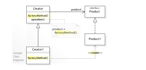
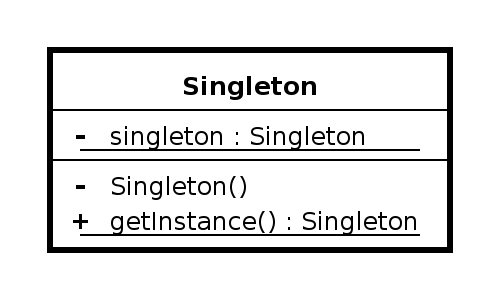
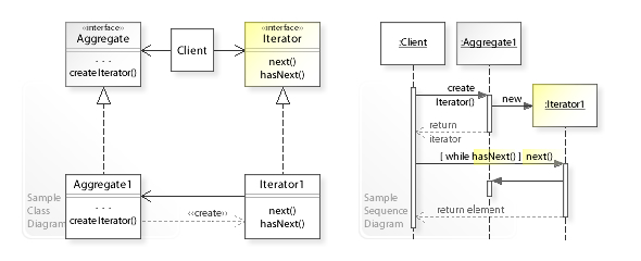
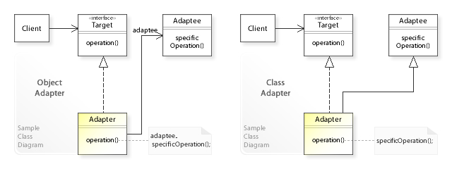
  • Design Patterns and Architectures
  • Computer Security
  • Advanced Object-Oriented Design
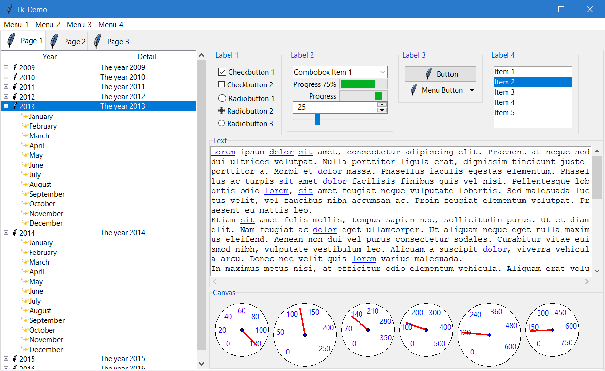
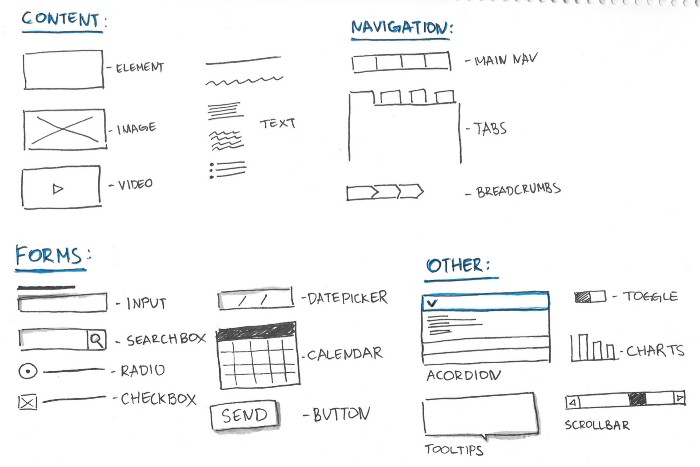
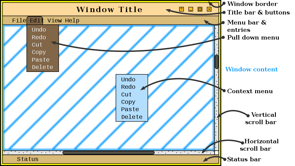
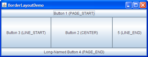
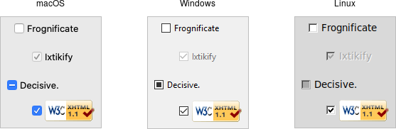
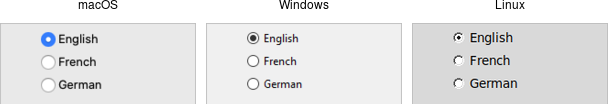
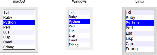
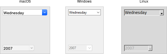
  • GUI Programming
  • Event-Driven Programming
  • Professional Communication and Collaboration

Student Learning Outcomes

After completing this course, a successful student will be able to:

  • Develop code following industry best-practices for code style and documentation
  • Develop and execute unit tests that adequately test code for bugs and errors
  • Make use of tools to determine the code coverage of a set of unit tests
  • Make use of source code management tools to maintain and store a code base
  • Create a class library following the object-oriented paradigm that makes effective use of inheritance and polymorphism where appropriate
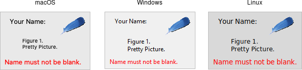
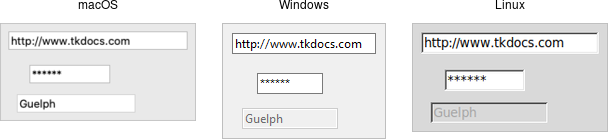
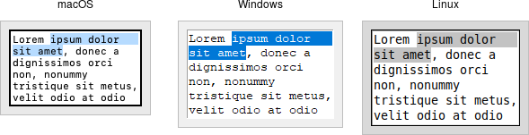
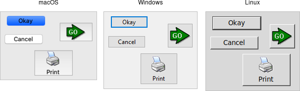
  • Develop a GUI for a given program that uses event-driven programming to respond to GUI events and manipulate underlying data models
  • Apply common software development methodologies, processes and design patterns to create software that performs a desired task or solves a problem
  • Communicate information about their code effectively with various audiences

Course Structure

These courses are being taught 100% online, and each module is self-paced. There may be some bumps in the road as we refine the overall course structure. Students will work at their own pace through a set of modules, with approximately one module being due each week. Material will be provided in the form of recorded videos, online tutorials, links to online resources, and discussion prompts. Each module will include a coding project or assignment, many of which will be graded automatically through Codio. Assignments may also include portions which will be graded manually via Canvas or other tools.

A common axiom in learner-centered teaching is “the person doing the work is the person doing the learning.” What this really means is that students primarily learn through grappling with the concepts and skills of a course while attempting to apply them. Simply seeing a demonstration or hearing a lecture by itself doesn’t do much in terms of learning. This is not to say that they don’t serve an important role - as they set the stage for the learning to come, helping you to recognize the core ideas to focus on as you work. The work itself consists of applying ideas, practicing skills, and putting the concepts into your own words.

The Work

There is no shortcut to becoming a great programmer. Only by doing the work will you develop the skills and knowledge to make you a successful computer scientist. This course is built around that principle, and gives you ample opportunity to do the work, with as much support as we can offer.

Tutorials, Quizzes & Examples: Each module will include many tutorial assignments, quizzes, and examples that will take you step-by-step through using a particular concept or technique. The point is not simply to complete the example, but to practice the technique and coding involved. You will be expected to implement these techniques on your own in the milestone assignment of the module - so this practice helps prepare you for those assignments.

Milestone Programming Assignments: Throughout the semester you will be building a non-trivial software project iteratively; every week a new milestone (a collection of features embodying a new version of a software application) will be due. Each milestone builds upon the prior milestone’s code base, so it is critical that you complete each milestone in a timely manner! This process also reflects the way software development is done in the real world - breaking large projects into more readily achievable milestones helps manage the development process.

Following along that real-world theme, programming assignments in this class will also be graded according to their conformance to coding style, documentation, and testing requirements. Each milestone’s rubric will include points assigned to each of these factors. It is not enough to simply write code that compiles and meets the specification; good code is readable, maintainable, efficient, and secure. The principles and practices of Object-Oriented programming that we will be learning in this course have been developed specifically to help address these concerns.

Concept Quizzes: There will be a couple of concept quizzes throughout the semester to check your understanding of various programming topics. These will allow you to demonstrate your problem-solving skills and your ability to apply what you’ve learned to novel situations.

Final Project: At the end of this course, you will design and develop a final project of your choosing to demonstrate your ability. This project can link back to your interest or other fields, and will serve as a capstone project for the Computational Core program.

Grading

In theory, each student begins the course with an A. As you submit work, you can either maintain your A (for good work) or chip away at it (for less adequate or incomplete work). In practice, each student starts with 0 points in the gradebook and works upward toward a final point total earned out of the possible number of points. In this course, each assignment constitutes a portion of the final grade, as detailed below:

  • 10% - Tutorials & Quizzes
  • 10% - Examples
  • 40% - Programming Project Milestones
  • 15% - Concept Quizzes
  • 25% - Final Project

Up to 5% of the total grade in the class is available as extra credit. See the Extra Credit - Bug Bounty & Extra Credit - Helping Hands assignments for details.

Letter grades will be assigned following the standard scale:

  • 90% - 100% → A
  • 80% - 89.99% → B
  • 70% - 79.99% → C
  • 60% - 69.99% → D
  • 00% - 59.99% → F

Submission, Regrading, and Early Grading Policy

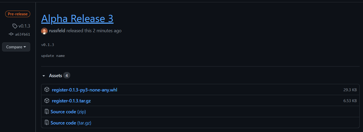
As a rule, submissions in this course will not be graded until after they are due, even if submitted early. Students may resubmit assignments many times before the due date, and only the latest submission will be graded. For assignments submitted via GitHub release tag, only the tagged release that was submitted to Canvas will be graded, even if additional commits have been made. Students must create a new tagged release and resubmit that tag to have it graded for that assignment.

Once an assignment is graded, students are not allowed to resubmit the assignment for regrading or additional credit without special permission from the instructor to do so. In essence, students are expected to ensure their work is complete and meets the requirements before submission, not after feedback is given by the instructor during grading. However, students should use that feedback to improve future assignments and milestones.

For the programming project milestones, it is solely at the discretion of the instructor whether issues noted in the feedback for a milestone will result in grade deductions in a later milestones if they remain unresolved, though the instructor will strive to give students ample time to resolve issues before any additional grade deductions are made.

Likewise, students may ask questions of the instructor while working on the assignment and receive help, but the instructor will not perform a full code review nor give grading-level feedback until after the assignment is submitted and the due date has passed. Again, students are expected to be able to make their own judgments on the quality and completion of an assignment before submission.

That said, a student may email the instructor to request early grading on an assignment before the due date, in order to move ahead more quickly. The instructor’s receipt of that email will effectively mean that the assignment for that student is due immediately, and all limitations above will apply as if the assignment’s due date has now passed.

Collaboration Policy

In this course, all work submitted by a student should be created solely by the student without any outside assistance beyond the instructor and TA/GTAs. Students may seek outside help or tutoring regarding concepts presented in the course, but should not share or receive any answers, source code, program structure, or any other materials related to the course. Learning to debug coding problems is a vital skill, and students should strive to ask good questions and perform their own research instead of just sharing broken source code when asking for assistance.

Late Work

Warning

Read this late work policy very carefully! If you are unsure how to interpret it, please contact the instructors via email. Not understanding the policy does not mean that it won’t apply to you!

Since this course is entirely online, students may work at any time and at their own pace through the modules. However, to keep everyone on track, there will be approximately one module due each week. Each graded item in the module will have a specific due date specified. Any assignment submitted late will have that assignment’s grade reduced by 10% of the total possible points on that project for each day it is late. This penalty will be assessed automatically in the Canvas gradebook. For the purposes of record keeping, a combination of the time of a submission via Canvas and the creation of a release in GitHub will be used to determine if the assignment was submitted on time.

However, even if a module is not submitted on time, it must still be completed before a student is allowed to begin the next module. So, students should take care not to get too far behind, as it may be very difficult to catch up.

Finally, all course work must be submitted on or before the last day of the semester in which the student is enrolled in the course in order for it to be graded on time.

If you have extenuating circumstances, please discuss them with the instructor as soon as they arise so other arrangements can be made. If you find that you are getting behind in the class, you are encouraged to speak to the instructor for options to make up missed work.

Incomplete Policy

Students should strive to complete this course in its entirety before the end of the semester in which they are enrolled. However, since retaking the course would be costly and repetitive for students, we would like to give students a chance to succeed with a little help rather than immediately fail students who are struggling.

If you are unable to complete the course in a timely manner, please contact the instructor to discuss an incomplete grade. Incomplete grades are given solely at the instructor’s discretion. See the official K-State Grading Policy for more information. In general, poor time management alone is not a sufficient reason for an incomplete grade.

Unless otherwise noted in writing on a signed Incomplete Agreement Form , the following stipulations apply to any incomplete grades given in Computational Core courses:

  1. Students may receive at most two incompletes in Computational Core courses throughout their time in the program
  2. Students will be given 6 calendar weeks from the end of the enrolled semester’s finals week to complete the course
  3. Any modules in a future CC course which depend on incomplete work will not be accessible until the previous course is finished
  4. For example, if a student is given an incomplete in CC 210, then all modules in CC 310 will be inaccessible until CC 210 is complete
  5. Students understand that access to instructor and GTA assistance may be limited after the end of an academic semester due to holidays and other obligations
  6. If a student fails to resolve an incomplete grade after 6 weeks, they will be assigned an ‘F’ in the course. In addition, they will be dropped from any other Computational Core courses which require the failed course as a prerequisite or corequisite.

To participate in this course, students must have access to a modern web browser and broadband internet connection. All course materials will be provided via Canvas and Codio. Modules may also contain links to external resources for additional information, such as programming language documentation.

Students will make use of GitHub or GitLab for source code management.

Students may choose to do some development work on their own computer. The recommended software is Visual Studio Code along with access to a system running Ubuntu . For Windows systems, Ubuntu can be installed via the Windows Subsystem for Linux . For Mac systems, Ubuntu can be installed in a virtual machine through VirtualBox .

Subject to Change

The details in this syllabus are not set in stone. Due to the flexible nature of this class, adjustments may need to be made as the semester progresses, though they will be kept to a minimum. If any changes occur, the changes will be posted on the Canvas page for this course and emailed to all students. All changes may also be posted to Canvas.

Standard Syllabus Statements

Info

The statements below are standard syllabus statements from K-State and our program. The latest versions are available online here .

Academic Honesty

Kansas State University has an Honor and Integrity System based on personal integrity, which is presumed to be sufficient assurance that, in academic matters, one’s work is performed honestly and without unauthorized assistance. Undergraduate and graduate students, by registration, acknowledge the jurisdiction of the Honor and Integrity System. The policies and procedures of the Honor and Integrity System apply to all full and part-time students enrolled in undergraduate and graduate courses on-campus, off-campus, and via distance learning. A component vital to the Honor and Integrity System is the inclusion of the Honor Pledge which applies to all assignments, examinations, or other course work undertaken by students. The Honor Pledge is implied, whether or not it is stated: “On my honor, as a student, I have neither given nor received unauthorized aid on this academic work.” A grade of XF can result from a breach of academic honesty. The F indicates failure in the course; the X indicates the reason is an Honor Pledge violation.

For this course, a violation of the Honor Pledge will result in sanctions such as a 0 on the assignment or an XF in the course, depending on severity. Actively seeking unauthorized aid, such as posting lab assignments on sites such as Chegg or StackOverflow, or asking another person to complete your work, even if unsuccessful, will result in an immediate XF in the course.

This course assumes that all your course work will be done by you. Use of AI text and code generators such as ChatGPT and GitHub Copilot in any submission for this course is strictly forbidden unless explicitly allowed by your instructor. Any unauthorized use of these tools without proper attribution is a violation of the K-State Honor Pledge .

We reserve the right to use various platforms that can perform automatic plagiarism detection by tracking changes made to files and comparing submitted projects against other students’ submissions and known solutions. That information may be used to determine if plagiarism has taken place.

Students with Disabilities

At K-State it is important that every student has access to course content and the means to demonstrate course mastery. Students with disabilities may benefit from services including accommodations provided by the Student Access Center. Disabilities can include physical, learning, executive functions, and mental health. You may register at the Student Access Center or to learn more contact:

Students already registered with the Student Access Center please request your Letters of Accommodation early in the semester to provide adequate time to arrange your approved academic accommodations. Once SAC approves your Letter of Accommodation it will be e-mailed to you, and your instructor(s) for this course. Please follow up with your instructor to discuss how best to implement the approved accommodations.

Expectations for Conduct

All student activities in the University, including this course, are governed by the Student Judicial Conduct Code as outlined in the Student Governing Association By Laws , Article V, Section 3, number 2. Students who engage in behavior that disrupts the learning environment may be asked to leave the class.

Mutual Respect and Inclusion in K-State Teaching & Learning Spaces

At K-State, faculty and staff are committed to creating and maintaining an inclusive and supportive learning environment for students from diverse backgrounds and perspectives. K-State courses, labs, and other virtual and physical learning spaces promote equitable opportunity to learn, participate, contribute, and succeed, regardless of age, race, color, ethnicity, nationality, genetic information, ancestry, disability, socioeconomic status, military or veteran status, immigration status, Indigenous identity, gender identity, gender expression, sexuality, religion, culture, as well as other social identities.

Faculty and staff are committed to promoting equity and believe the success of an inclusive learning environment relies on the participation, support, and understanding of all students. Students are encouraged to share their views and lived experiences as they relate to the course or their course experience, while recognizing they are doing so in a learning environment in which all are expected to engage with respect to honor the rights, safety, and dignity of others in keeping with the K-State Principles of Community .

If you feel uncomfortable because of comments or behavior encountered in this class, you may bring it to the attention of your instructor, advisors, and/or mentors. If you have questions about how to proceed with a confidential process to resolve concerns, please contact the Student Ombudsperson Office . Violations of the student code of conduct can be reported using the Code of Conduct Reporting Form . You can also report discrimination, harassment or sexual harassment , if needed.

Netiquette

Info

This is our personal policy and not a required syllabus statement from K-State. It has been adapted from this statement from K-State Global Campus, and theRecurse Center Manual . We have adapted their ideas to fit this course.

Online communication is inherently different than in-person communication. When speaking in person, many times we can take advantage of the context and body language of the person speaking to better understand what the speaker means, not just what is said. This information is not present when communicating online, so we must be much more careful about what we say and how we say it in order to get our meaning across.

Here are a few general rules to help us all communicate online in this course, especially while using tools such as Canvas or Discord:

  • Use a clear and meaningful subject line to announce your topic. Subject lines such as “Question” or “Problem” are not helpful. Subjects such as “Logic Question in Project 5, Part 1 in Java” or “Unexpected Exception when Opening Text File in Python” give plenty of information about your topic.
  • Use only one topic per message. If you have multiple topics, post multiple messages so each one can be discussed independently.
  • Be thorough, concise, and to the point. Ideally, each message should be a page or less.
  • Include exact error messages, code snippets, or screenshots, as well as any previous steps taken to fix the problem. It is much easier to solve a problem when the exact error message or screenshot is provided. If we know what you’ve tried so far, we can get to the root cause of the issue more quickly.
  • Consider carefully what you write before you post it. Once a message is posted, it becomes part of the permanent record of the course and can easily be found by others.
  • If you are lost, don’t know an answer, or don’t understand something, speak up! Email and Canvas both allow you to send a message privately to the instructors, so other students won’t see that you asked a question. Don’t be afraid to ask questions anytime, as you can choose to do so without any fear of being identified by your fellow students.
  • Class discussions are confidential. Do not share information from the course with anyone outside of the course without explicit permission.
  • Do not quote entire message chains; only include the relevant parts. When replying to a previous message, only quote the relevant lines in your response.
  • Do not use all caps. It makes it look like you are shouting. Use appropriate text markup (bold, italics, etc.) to highlight a point if needed.
  • No feigning surprise. If someone asks a question, saying things like “I can’t believe you don’t know that!” are not helpful, and only serve to make that person feel bad.
  • No “well-actually’s.” If someone makes a statement that is not entirely correct, resist the urge to offer a “well, actually…” correction, especially if it is not relevant to the discussion. If you can help solve their problem, feel free to provide correct information, but don’t post a correction just for the sake of being correct.
  • Do not correct someone’s grammar or spelling. Again, it is not helpful, and only serves to make that person feel bad. If there is a genuine mistake that may affect the meaning of the post, please contact the person privately or let the instructors know privately so it can be resolved.
  • Avoid subtle -isms and microaggressions. Avoid comments that could make others feel uncomfortable based on their personal identity. See the syllabus section on Diversity and Inclusion above for more information on this topic. If a comment makes you uncomfortable, please contact the instructor.
  • Avoid sarcasm, flaming, advertisements, lingo, trolling, doxxing, and other bad online habits. They have no place in an academic environment. Tasteful humor is fine, but sarcasm can be misunderstood.

As a participant in course discussions, you should also strive to honor the diversity of your classmates by adhering to the K-State Principles of Community .

SafeZone Ally

I am part of the SafeZone community network of trained K-State faculty/staff/students who are available to listen and support you. As a SafeZone Ally, I can help you connect with resources on campus to address problems you face that interfere with your academic success, particularly issues of sexual violence, hateful acts, or concerns faced by individuals due to sexual orientation/gender identity. My goal is to help you be successful and to maintain a safe and equitable campus.

Discrimination, Harassment, and Sexual Harassment

Kansas State University is committed to maintaining academic, housing, and work environments that are free of discrimination, harassment, and sexual harassment. Instructors support the University’s commitment by creating a safe learning environment during this course, free of conduct that would interfere with your academic opportunities. Instructors also have a duty to report any behavior they become aware of that potentially violates the University’s policy prohibiting discrimination, harassment, and sexual harassment, as outlined by PPM 3010 .

If a student is subjected to discrimination, harassment, or sexual harassment, they are encouraged to make a non-confidential report to the University’s Office for Institutional Equity (OIE) using the online reporting form . Incident disclosure is not required to receive resources at K-State. Reports that include domestic and dating violence, sexual assault, or stalking, should be considered for reporting by the complainant to the Kansas State University Police Department or the Riley County Police Department . Reports made to law enforcement are separate from reports made to OIE. A complainant can choose to report to one or both entities. Confidential support and advocacy can be found with the K-State Center for Advocacy, Response, and Education (CARE) . Confidential mental health services can be found with Lafene Counseling and Psychological Services (CAPS) . Academic support can be found with the Office of Student Life (OSL) . OSL is a non-confidential resource. OIE also provides a comprehensive list of resources on their website. If you have questions about non-confidential and confidential resources, please contact OIE at equity@ksu.edu or (785) 532–6220.

Academic Freedom Statement

Kansas State University is a community of students, faculty, and staff who work together to discover new knowledge, create new ideas, and share the results of their scholarly inquiry with the wider public. Although new ideas or research results may be controversial or challenge established views, the health and growth of any society requires frank intellectual exchange. Academic freedom protects this type of free exchange and is thus essential to any university’s mission.

Moreover, academic freedom supports collaborative work in the pursuit of truth and the dissemination of knowledge in an environment of inquiry, respectful debate, and professionalism. Academic freedom is not limited to the classroom or to scientific and scholarly research, but extends to the life of the university as well as to larger social and political questions. It is the right and responsibility of the university community to engage with such issues.

Campus Safety

Kansas State University is committed to providing a safe teaching and learning environment for student and faculty members. In order to enhance your safety in the unlikely case of a campus emergency make sure that you know where and how to quickly exit your classroom and how to follow any emergency directives. Current Campus Emergency Information is available at the University’s Advisory webpage.

Weapons Policy

Kansas State University prohibits the possession of firearms, explosives, and other weapons on any University campus, with certain limited exceptions, including the lawful concealed carrying of handguns, as provided in the University Weapons Policy .

You are encouraged to take the online weapons policy education module to ensure you understand the requirements of the policy, including the requirements related to concealed carrying of handguns on campus. Students possessing a concealed handgun on campus must be lawfully eligible to carry and either at least 21 years of age or a licensed individual who is 18-21 years of age. All carrying requirements of the policy must be observed in this class, including but not limited to the requirement that a concealed handgun be completely hidden from view, securely held in a holster that meets the specifications of the policy, carried without a chambered round of ammunition, and that any external safety be in the “on” position.

If an individual carries a concealed handgun in a personal carrier such as a backpack, purse, or handbag, the carrier must remain within the individual’s exclusive and uninterrupted control. This includes wearing the carrier with a strap, carrying or holding the carrier, or setting the carrier next to or within the immediate reach of the individual.

During this course, you will be required to engage in activities, such as interactive examples or sharing work on the whiteboard, that may require you to separate from your belongings, and thus you should plan accordingly.

Each individual who lawfully possesses a handgun on campus shall be wholly and solely responsible for carrying, storing and using that handgun in a safe manner and in accordance with the law, Board policy and University policy. All reports of suspected violation of the weapons policy are made to the University Police Department by picking up any Emergency Campus Phone or by calling 785-532-6412.

Student Resources

K-State has many resources to help contribute to student success. These resources include accommodations for academics, paying for college, student life, health and safety, and others. Check out the Student Guide to Help and Resources: One Stop Shop for more information.

Student Academic Creations

Student academic creations are subject to Kansas State University and Kansas Board of Regents Intellectual Property Policies. For courses in which students will be creating intellectual property, the K-State policy can be found at University Handbook, Appendix R: Intellectual Property Policy and Institutional Procedures (part I.E.) . These policies address ownership and use of student academic creations.

Mental Health

Your mental health and good relationships are vital to your overall well-being. Symptoms of mental health issues may include excessive sadness or worry, thoughts of death or self-harm, inability to concentrate, lack of motivation, or substance abuse. Although problems can occur anytime for anyone, you should pay extra attention to your mental health if you are feeling academic or financial stress, discrimination, or have experienced a traumatic event, such as loss of a friend or family member, sexual assault or other physical or emotional abuse.

If you are struggling with these issues, do not wait to seek assistance.

For Kansas State Salina Campus:

For Global Campus/K-State Online:

  • K-State Online students have free access to mental health counseling with My SSP - 24/7 support via chat and phone.
  • The Office of Student Life can direct you to additional resources.

University Excused Absences

K-State has a University Excused Absence policy (Section F62) . Class absence(s) will be handled between the instructor and the student unless there are other university offices involved. For university excused absences, instructors shall provide the student the opportunity to make up missed assignments, activities, and/or attendance specific points that contribute to the course grade, unless they decide to excuse those missed assignments from the student’s course grade. Please see the policy for a complete list of university excused absences and how to obtain one. Students are encouraged to contact their instructor regarding their absences.

© The materials in this online course fall under the protection of all intellectual property, copyright and trademark laws of the U.S. The digital materials included here come with the legal permissions and releases of the copyright holders. These course materials should be used for educational purposes only; the contents should not be distributed electronically or otherwise beyond the confines of this online course. The URLs listed here do not suggest endorsement of either the site owners or the contents found at the sites. Likewise, mentioned brands (products and services) do not suggest endorsement. Students own copyright to what they create.

Subsections of Spring 2024 Syllabus

Plagiarism Policy

YouTube Video

Resources

Video Script

“On my honor, as a student, I have neither given nor received unauthorized aid on this academic work.” - K-State Honor Pledge

Plagiarism is a very serious concern in this course, and something that we do not take lightly. Computer programs and code are especially easy targets for plagiarism due to how easy it is to copy and manipulate code in such a way that it is unrecognizable as the original source but still performs correctly.

At its core, plagiarism is taking someone else’s work and passing it off as your own without giving appropriate credit to the original source. As a student at K-State, you are bound by the K-State Honor Code not to accept any unauthorized aid, and this includes plagiarized code.

When it comes to plagiarism in computer code, there is a fine line between using resources appropriately and copying code. In this program, you should strive to avoid plagiarism issues by doing the following:

  1. Do not search for or use any complete solutions to projects in this course found online or from fellow students.
  2. Small portions of code may be used or adapted from an online source with proper citation. To cite a piece of code, include a code comment section above it that contains the original source URL and a description of why it was used.

In general, copying or adapting small pieces of code to perform auxiliary functions in the assignment is permitted. Copying or adapting code that is the general goal of the assignment should be avoided. For example, if the assignment is to create a bubble sort algorithm, you should write the algorithm from scratch yourself since that is the goal of the assignment. If the assignment is to create a program for displaying data that you feel should be sorted, you may choose to adapt an existing sorting algorithm for your needs (or use one from a library).

If you aren’t sure about whether it is OK to use an online resource or piece of code in this course, please contact the instructors using the course discussion forums or help email address. You will not get in trouble for asking, and it will help you determine what the best course of action is. Plagiarism can really only occur when you submit the assignment for grading, so you are welcome to ask for clarification or a judgement on whether a particular usage is acceptable at any time before you submit the assignment.

Codio has features that will compare your submissions against those of your fellow students. Any submissions with a high degree of similarity may be subjected to additional scrutiny by the instructors to determine if plagiarism has occurred.

In this course, any violation of the K-State Honor Code will result in a 0 on that assignment and a report made to the K-State Honor Council. A second violation will result in an XF in this course, as well as any additional sanctions imposed by the K-State Honor Council.

For more information on the K-State Honor & Integrity system, please visit their website , which is linked in the resources section below this video.

Codio Projects

YouTube Video

Resources

Video Script

At this point, you should have completed the “Hello Real World” example project. This module contains GitHub Classroom assignments and Codio projects for the rest of this course. In this video, I’ll briefly explain what these are for and how they work. As always, if you have any questions or are unsure what to do, contact the instructors via cc410-help for assistance.

Looking at this module, the first item you should see is the Codio Playground. This is a blank Codio project that you can use for just about anything. You can explore Codio’s interface, test new code snippets, and try new development tools. This Codio project starts with exactly the same setup as the two other projects in this course, so you’ll have the same experience here as in the others. Finally, if you ever have issues or want to start over, just contact the instructors and ask them to reset your playground project. Of course, you’ll lose all your content, but it is a great way to try things and make mistakes until you get them right.

The next four items in this module are for the two major programming projects in this course - the restaurant project and the final project. Before we discuss those individually, let’s talk about what they have in common. Both of those projects have a matching assignment in GitHub classroom that you’ll need to accept, just like you did for the Hello Real World project. Once you’ve accepted that assignment, you can clone the assignment’s repository into the associated Codio project and get started coding. Feel free to follow the guide from the Hello Real World project to set up your environment. You can even copy and paste the content from Hello Real World into these projects and use that as a starting point! For these two projects, you’ll be using the same Codio project all semester, which can always be accessed through this module. We’ve placed it toward the top of the module list so it is easy to get to quickly. Once you’ve completed a milestone for a project, you’ll follow the steps you learned in the Hello Real World project to create a release on GitHub, and then submit that URL via Canvas to complete the milestone assignment. The instructors will give you grades and feedback within a couple of days, but you’ll be able to move on and start working on the next milestone immediately. You can always update your release later with a new version if needed. Finally, this course will move pretty quickly, so you can expect to complete around 1 project milestone each week, in addition to the tutorials and examples for that week’s module. Most examples won’t be nearly as big as Hello Real World, but they’ll still require an hour or so of work.

Now, let’s talk about the individual projects. First, we have the restaurant project. In this project, we’ll build a point-of-sale system for a fictional restaurant. This is a guided project, and you’ll follow along with the tutorials and examples to complete each milestone. We’ll show you be basics, and then you’ll continue to build upon that in each milestone. There will be several milestones to complete for this project, and they include building a class library using object-oriented programming concepts, building a useful graphical user interface or GUI, and learning how to access and build your own web APIs to extend the usefulness of the project. So, starting in Module 2, you’ll learn all about building a class library and start working toward the first milestone.

There will also be a final project in this course. This is a self-directed programming project, where you get to choose the project and what it will do. This project will include just a few milestones spread throughout the course, roughly designed to coincide with work you are doing on the restaurant project. For this project, you will be asked to find a topic that fits with your interests. A good place to look would be within your major or concentration, but it could be anything that interests you. At the end of the semester, you’ll develop a presentation and present your work to the class. For students completing the CS certificate or in the integrated CS program, this project will also serve as a capstone project for those programs. Watch the course announcements and later modules for more information about the structure and requirements of the final project.

So, when you are ready to begin a project, where should you start? Here’s a quick rundown of the steps we recommend following. First, accept the assignment via GitHub classroom to create your own private repository for the code. Then, open the associated Codio project from this module, and follow the steps outlined in the Hello Real World example to set up the project. When you are asked to clone the GitHub repository, make sure you use the URL for correct assignment repository that you accepted in an earlier step. Then, once your project is all set up, write your code in Codio and make commits to the Git repository as you go. We highly recommend committing code often, usually many times per day, as it makes it easier to undo mistakes and fix bugs later on. Once you’ve completed work on a project milestone, follow the steps in the Hello Real World example project to create a GitHub release, and then submit the URL for that release to the project milestone assignment on Canvas. You will not submit the Codio project like you did in earlier CC courses - instead, you’ll be able to keep using the same Codio project for the entire semester. You’ll just create and submit additional GitHub releases for later milestones.

Hopefully that all makes sense, but if not feel free to forge ahead and ask questions as you go. At this point, you are ready to skip ahead to Module 2 in Canvas and start there. In that module, you’ll complete a tutorial and example, and then you’ll see the requirements for a project milestone. Once you are there, come back to this module and open up the relevant Codio project to start working on that milestone. Once you’ve completed work on that milestone, create a release in GitHub and submit the URL back in the milestone assignment in the module you are working in to complete it and move on to the next module. Once you’ve done this process a couple of times, it should be pretty easy to follow.

Finally, don’t forget to check the bottom of the Modules list in Canvas to find some additional content that may be useful in this course. We’ve included links to the textbooks for all prior CC courses, as well as a set of helpful Codio tutorials for learning the Linux command line. The first four are especially useful if you’ve not used Linux or the Linux terminal before. We’ll also be adding links to tutorials and helpful information for learning how to use tools like Git and GitHub, as well as some information for setting up your own integrated development environments, or IDEs, on your own computers. While all the work in this course can be done via Codio, you are welcome to use your own tools if you prefer, provided your project meets all the requirements. Basically, if it works in Codio, it should be fine.

Since this is a new course, we’re always looking for feedback. So, as you go through this course and work on the project milestones, please feel free to contact us via the cc410-help email address if you have any comments or suggestions for how we could better organize or explain the information in this course. You could even earn some “bug bounty” extra credit points!

So, feel free to move directly on to Module 2 in Canvas and start there, then come back here to begin working on the projects once you reach the appropriate points in the course. As always, if you have any questions, please let us know. Good luck!

Subsections of Codio Projects

Chapter I

OOP

Building Programs from Classes and Objects!

Subsections of OOP

Chapter 1

Hello Real World

Hello World, but like the pros do it!

Subsections of Hello Real World

Welcome

Welcome to CC 410 - Advanced Programming. This course is designed to be a capstone experience at the end of the Computational Core program, building upon our prior knowledge and experience to help us become a truly effective programmer. In this course, we’ll not only learn new skills and techniques, but we’ll try to pull back the curtain and explain the history of programming and why we do some of the things we do.

Big Ideas

In this course, we’re going to cover a lot of content. However, it can be grouped into a few big ideas in programming:

  • How can we write professional looking code that is easy for others to understand?
  • How can we effectively debug and test our programs to minimize the number of bugs?
  • What is object-oriented programming, really, and why is it so popular?
  • How can we develop programs that have a graphical user interface (GUI)?
  • What is event-driven programming, and how does it relate to the development of GUIs?
  • What are some common design patterns that we can use in our code?
  • How can we interface with applications on the Internet?
  • How do we design and develop our own programs from scratch to solve a particular problem?

We’ll spend some time covering each of these in more detail as we go through the course. In this module, we’ll start working on the first two - writing professional code and minimizing bugs through testing and debugging.

Getting Started

Before we dive too deeply into this topic, let’s take a step back and examine some of the history of programming that lead to our current state of the art that revolves around object-oriented programming. To do that, we’ll need to explore the software crisis and the topic of structured programming.

The Growth of Computing

Content Note

The content on this page was adapted from Nathan Bean’s CIS 400 course at K-State, with the author’s permission. That content is licensed under a Creative Commons BY-NC-SA license.

By this point, you should be familiar enough with the history of computers to be aware of the evolution from the massive room-filling vacuum tube implementations of ENIAC, UNIVAC, and other first-generation computers to transistor-based mainframes like the PDP-1, and the eventual introduction of the microcomputer (desktop computers that are the basis of the modern PC) in the late 1970s. Along with a declining size, each generation of these machines also cost less:

Machine Release Year Cost at Release Adjusted for Inflation
ENIAC 1945 $400,000 $5,288,143
UNIVAC 1951 $159,000 $1,576,527
PDP-1 1963 $120,000 $1,010,968
Commodore PET 1977 $795 $5,282
Apple II (4K RAM model) 1977 $1,298 $8,624
IBM PC 1981 $1,565 $4,438
Commodore 64 1982 $595 $1,589

This increase in affordability was also coupled with an increase in computational power. Consider the ENIAC, which computed at 100,000 cycles per second. In contrast, the relatively inexpensive Commodore 64 ran at 1,000,000 cycles per second, while the more pricey IBM PC ran 4,770,000 cycles per second.

Not surprisingly, governments, corporations, schools, and even individuals purchased computers in larger and larger quantities, and the demand for software to run on these platforms and meet these customers’ needs likewise grew. Moreover, the sophistication expected from this software also grew. Edsger Dijkstra described it in these terms:

The major cause of the software crisis is that the machines have become several orders of magnitude more powerful! To put it quite bluntly: as long as there were no machines, programming was no problem at all; when we had a few weak computers, programming became a mild problem, and now we have gigantic computers, programming has become an equally gigantic problem. – Edsger Dijkstra, The Humble Programmer (EWD340), Communications of the ACM

Coupled with this rising demand for programs was a demand for skilled software developers, as reflected in the following table of graduation rates in programming-centric degrees (the dashed line represents the growth of all bachelor degrees, not just computer-related ones):

Annual Computer-Related Bachelor Degrees Awarded in the US Annual Computer-Related Bachelor Degrees Awarded in the US

Unfortunately, this graduation rate often lagged far behind the demand for skilled graduates, and was marked by several periods of intense growth (the period from 1965 to 1985, 1995-2003, and the current surge beginning around 2010). During these surges, it was not uncommon to see students hired directly into the industry after only a course or two of learning programming (coding boot camps are a modern equivalent of this trend).

All of these trends contributed to what we now call the Software Crisis.

The Software Crisis

Content Note

The content on this page was adapted from Nathan Bean’s CIS 400 course at K-State, with the author’s permission. That content is licensed under a Creative Commons BY-NC-SA license.

YouTube Video

Video Materials

At the 1968 NATO Software Engineering Conference held in Garmisch Germany, the term “Software Crisis” was coined to describe the current state of the software development industry, where common problems included:

  • Projects that ran over-budget
  • Projects that ran over-time
  • Software that made inefficient use of calculations and memory
  • Software was of low quality
  • Software that failed to meet the requirements it was developed to meet
  • Projects that became unmanagable and code difficult to maintain
  • Software that never finished development

The software development industry sought to counter these problems through a variety of efforts:

  • The development of new programming languages with features intended to make it harder for programmers to make errors.
  • The development of Integrated Development Environments (IDEs) with developer-centric tools to aid in the software development process, including syntax highlighting, interactive debuggers, and profiling tools
  • The development of code repository tools like SVN and GIT
  • The development and adoption of code documentation standards
  • The development and adoption of program modeling languages like UML
  • The use of automated testing frameworks and tools to verify expected functionality
  • The adoption of software development practices that adopted ideas from other engineering disciplines

This course will seek to instill many of these ideas and approaches into your programming practice through adopting them in our everyday work. It is important to understand that unless these practices are used, the same problems that defined the software crisis continue to occur!

In fact, some software engineering experts suggest the software crisis isn’t over, pointing to recent failures like the Denver Airport Baggage System in 1995, the Ariane 5 Rocket Explosion in 1996, the German Toll Collect system canceled in 2003, the rocky healthcare.gov launch in 2013, and the massive vulnerabilities known as the Meltdown and Spectre exploits discovered in 2018.

Subsections of The Software Crisis

Language Evolution

Content Note

The content on this page was adapted from Nathan Bean’s CIS 400 course at K-State, with the author’s permission. That content is licensed under a Creative Commons BY-NC-SA license.

YouTube Video

Video Materials

One of the strategies that computer scientists employed to counter the software crisis was the development of new programing languages. These new languages would often 1) adopt new techniques intended to make errors harder to make while programming, and 2) remove problematic features that had existed in earlier languages.

A Fortran Example

Let’s take a look at a working (and in current use) program built using Fortran, one of the most popular programming languages at the onset of the software crisis. This software is the Environmental Policy Integrated Climate (EPIC) Model, created by researchers at Texas A&M:

Environmental Policy Integrated Climate (EPIC) model is a cropping systems model that was developed to estimate soil productivity as affected by erosion as part of the Soil and Water Resources Conservation Act analysis for 1980, which revealed a significant need for improving technology for evaluating the impacts of soil erosion on soil productivity. EPIC simulates approximately eighty crops with one crop growth model using unique parameter values for each crop. It predicts effects of management decisions on soil, water, nutrient and pesticide movements, and their combined impact on soil loss, water quality, and crop yields for areas with homogeneous soils and management. -- EPIC Homepage

You can download the raw source code and the accompanying documentation . Open and unzip the source code, and open a file at random using your favorite code editor. See if you can determine what it does, and how it fits into the overall application.

Try this with a few other files. What do you think of the organization? Would you be comfortable adding a new feature to this program?

New Language Features

You probably found the Fortran code in the example difficult to wrap your mind around - and that’s not surprising, as more recent languages have moved away from many of the practices employed in Fortran. Additionally, our computing environment has dramatically changed since this time.

Symbol Character Limits

One clear example is symbol names for variables and procedures (functions) - notice that in the Fortran code they are typically short and cryptic: RT, HU, IEVI, HUSE, and NFALL, for example. You’ve been told since your first class that variable and function names should express clearly what the variable represents or a function does. Would rainFall, dailyHeatUnits, cropLeafAreaIndexDevelopment, CalculateWaterAndNutrientUse(), CalculateConversionOfStandingDeadCropResidueToFlatResidue() be easier to decipher? (Hint: the documentation contains some of the variable notations in a list starting on page 70, and some in-code documentation of global variables occurs in MAIN_1102.f90.).

Believe it or not, there was an actual reason for short names in these early programs. A six character name would fit into a 36-bit register, allowing for fast dictionary lookups - accordingly, early version of FORTRAN enforced a limit of six characters for variable names1. However, it is easy to replace a symbol name with an automatically generated symbol during compilation, allowing for both fast lookup and human readability at a cost of some extra computation during compilation. This step is built into the compilation process of most current programming languages, allowing for arbitrary-length symbol names with no runtime performance penalty.

Structured Programming Paradigm

Another common change to programming languages was the removal of the GOTO statement, which allowed the program execution to jump to an arbitrary point in the code (much like a choose-your-own adventure book will direct you to jump to a page). The GOTO came to be considered too primitive, and too easy for a programmer to misuse 2.

However, the actual functionality of a GOTO statement remains in higher-order programming languages, abstracted into control-flow structures like conditionals, loops, and switch statements. This is the basis of structured programming , a paradigm adopted by all modern higher-order programming languages. Each of these control-flow structures can be represented by careful use of GOTO statements (and, in fact the resulting assembly code from compiling these languages does just that). The benefit is using structured programming promotes “reliability, correctness, and organizational clarity” by clearly defining the circumstances and effects fo code jumps 3.

Object-Orientation Paradigm

The object-orientation paradigm was similarly developed to make programming large projects easier and less error-prone. We’ll examine just how it seeks to do so in the next few chapters. But before we do, you might want to see how language popularity has fared since the onset of the software crisis, and how new languages have appeared and grown in popularity in this animated chart from Data is Beautiful:

YouTube Video

Interestingly, the four top languages in 2019 (Python, JavaScript, Java, and C#) all adopt the object-oriented paradigm - though the exact details of how they implement it vary dramatically.

The term “Object Orientation” was coined by Alan Kay while he was a graduate student in the late 60s. Alan Kay, Dan Ingalls, Adele Goldberg, and others created the first object-oriented language, Smalltalk , which became a very influential language from which many ideas were borrowed. To Alan, the essential core of object-orientation was three properties a language could possess: 4

  • Encapsulation
  • Message passing
  • Dynamic binding

We’ll take a look at each of these in the next few chapters.


  1. Weishart, Conrad (2010). “How Long Can a Data Name Be?”  ↩︎

  2. Dijkstra, Edgar (1968). “Go To Statement Considered Harmful”  ↩︎

  3. Wirth, Nicklaus (1974). “On the Composition of Well-Structured Programs”  ↩︎

  4. Eric Elliot, “The Forgotten History of Object-Oriented Programming,” Medium, Oct. 31, 2018. ↩︎

Subsections of Language Evolution

Writing Professional Code

YouTube Video

Video Materials

As we saw earlier in this module, the software development industry adopted many new processes and ideas to help combat the issues that arose during the software crisis. One of the major things they focused on was how to write code that is easy to understand, easy to maintain, and works as intended with a minimal amount of bugs. Let’s review a few of the concepts that came from those efforts, which we’ll learn more about throughout this semester.

Object-Oriented Programming

The use of object-oriented programming languages was one major outcome of the software crisis. An object-oriented language allows developers to build code that represents real-world concepts and ideas, making it easier to reason about large software programs. In addition, the concept of encapsulation helped ensure data stored and manipulated by one part of the program wasn’t inadvertently changed by a bug in another part. Finally, through message passing and dynamic binding, we could write more advanced functions that allowed our code to be very modularized, flexible, and highly reusable. We’ll spend the next several modules in this course covering object-oriented programming in much greater detail.

Unit Testing

Another major movement in the software industry was toward the use of automated testing frameworks and the use of unit testing. Unit testing involves writing detailed tests for small units of a program’s source code, often individual functions, that exercise the expected functionality of the code as well as checking for any edge cases or expected errors.

In theory, if the unit tests are properly written and perform all possible operations that the code should perform, than any code passing the tests should be considered complete and ready for use. Of course, coming up with a set of unit tests that can account for all possible scenarios is just as impossible as writing software that doesn’t contain any bugs, but it can be a great step toward writing better software.

A common software development methodology today is test-driven development or TDD. In test-driven development , the unit tests are developed first, based on the software specification, before the source code is ever written. In that way, it is easy to know if the software actually does what the requirements says it should, instead of the test simply being written to match the code that exists. (It is shockingly common for unit tests to be written based on the code it should test, which is equivalent of looking at the answers when doing a word scramble - you’ll find what you expect to find, but won’t actually learn anything useful from it.)

Another useful feature of unit tests is the ability to re-run tests on the program after an update has been developed, which is known as regression testing. If the program previously passed all available unit tests, then failed some of those tests after an update, we know that we introduced some unintended bugs in the code that can be repaired before publishing an update. In that way, we can avoid sending out an update that ends up making things even worse.

Code Coverage

Along with unit testing, another useful technique is calculating the code coverage of a set of tests. Ideally, you’d like to make sure that each and every line of code in the program is executed by at least one test - otherwise, how can you really say that that line does what it should? This is especially difficult in programs that contain multiple conditional statements and loops, or any code that checks for and handles exceptions.

There are various ways to measure code coverage , including this list from Wikipedia:

  • Function coverage - has every function been called?
  • Statement coverage - has every statement been executed?
  • Edge coverage - has every edge in the control flow graph been executed?
  • Branch coverage - has every branch in each control structure been executed?
  • Condition coverage - has every boolean expression been evaluated to both true and false?

There are various different ways to measure code coverage that we’ll discuss later in this course, but for now we’ll just look at statement coverage. Thankfully, there are some great tools for computing the code coverage of a set of unit tests. Our goal is always to get as close to 100% coverage as possible.

Documentation

Another major focus among professional coders is the inclusion of documentation directly in the source code itself. Many languages, such as Java, Python, and C#, include standards for documenting what various pieces of the code are for. This includes each individual source code file, classes, functions, attributes, and more. In many cases, this is done by including specially structured code comments in various places throughout the source code.

To make those comments easier to read and understand, many languages also include tools to automatically create developer documents based on those comments. A prime example of this is the Java API Documentation , which is nearly entirely generated directly from comments in the Java source code. In fact, you can compare the source code for the ArrayList class and the ArrayList Documentation in the Java API to get an idea of how this works.

Static Code Analysis

Finally, there are many tools available today that can perform static code analysis of source code, helping developers find and fix errors without ever even compiling and running the code. Some static code analysis tools are quite powerful, able to find logic errors or completely validate that the software meets a specification. These tools are commonly used in the development of critical software components, such as medical devices and avionics for aircraft, but they are also quite difficult to use.

In this course, we’re going to focus on a simpler form of static code analysis that will help us maintain good coding style. These tools are sometimes commonly referred to as “linters,” named for the old Unix ’lint’ tool that performed this task for code written in the C programming language. Of course, the use of the term “lint” is a reference to the tiny bits of fiber and fuzz that are shed by clothing, with the idea that by removing the “lint” that makes our code messy, we can have code that is cleaner and easier to read and maintain.

In fact, you may have already encountered these tools in your programming experience. Development environments such as the one used by Codio, as well as other integrated development environments (IDEs) such as Visual Studio Code, PyCharm, IntelliJ, and others all include support for static code analysis. Usually it takes the form of helpful error messages that show simple syntax and usage errors.

In this course, we’ll learn how to use some more powerful static code analysis tools to enforce a standard coding style across all of our source code. A [coding style] can be thought of as roughly equivalent to a dialect of a spoken or written language - it deals with common conventions and usage, beyond just the simple definitions and syntax rules of the language itself. By following a standardized style, our code will be easier to read and maintain for any developer who is familiar with that style.

Subsections of Writing Professional Code

Hello Real World

Example Videos

Based on the previous page, it sounds like writing professional code can be quite difficult. There are so many tools and concepts to keep track of, and, in fact, you may end up spending just as much time working with everything else around your code as you do writing the code itself. The benefit of all of this work comes later, when you have to update or maintain the code. If you’ve done a good job writing unit tests, checking for coverage, documenting and styling your code, you’ll end up with fewer bugs overall, and hopefully it will be easier to patch and update the code over the long term that it is in use.

Thankfully, in this course, we’re going to start small in this module with a new project we’re calling “Hello Real World.”

Hello Real World

Most programmers can recall the simple “Hello World” program they wrote when learning to program. For many of us, it is the first program we learned to write, and usually the first thing we write when learning a new language. It is almost a sacred tradition!

We’re going to build upon that in this module by learning to write a “Hello World” program of our own, but one that meets the following requirements:

  1. It must be fully object-oriented, with the code placed within a method that is inside of a class, which is part of a package.
  2. The code must include unit tests that fully verify that the code works properly in all cases.
  3. The unit tests must achieve 100% code coverage of the source code.
  4. The source code must contain full documentation for each file, class, and method, as defined by the language’s standard for in-code documentation.
  5. The source code must pass all checks enforced through static code analysis based on a common coding style for the language.
  6. The entire process should be easily executable at-will from the terminal, while providing opportunities for future full automation.
  7. The resulting code should be stored in a version control software system.

That’s quite a tall order, but this is really how a professional software developer would approach writing good and maintainable code. In some languages, such as Java, a few parts of this process are pretty straightforward - Java is already fully object-oriented by default, and Java uses a common standard for creating in-code documentation. Other languages, such as Python, end up becoming more complex to work with as more requirements are added. For Python developers, a simple “Hello World” program is a single line of code, whereas this set of requirements requires multiple files to properly create a Python package. In addition, the Python language itself does not define a common standard for in-code documentation, so we must rely on external resources to determine what coding style we should follow.

Thankfully, we’ll go through this entire process step by step in the example portion of this module, and you’ll be able to follow along and build your own version of “Hello Real World.”

Subsections of Hello Real World

Summary

Content Note

Portions of the content on this page were adapted from Nathan Bean’s CIS 400 course at K-State, with the author’s permission. That content is licensed under a Creative Commons BY-NC-SA license.

In this chapter, we’ve discussed the environment in which object-orientation emerged. Early computers were limited in their computational power, and languages and programming techniques had to work around these limitations. Similarly, these computers were very expensive, so their purchasers were very concerned about getting the largest possible return on their investment. In the words of Niklaus Wirth:

Tricks were necessary at this time, simply because machines were built with limitations imposed by a technology in its early development stage, and because even problems that would be termed "simple" nowadays could not be handled in a straightforward way. It was the programmers' very task to push computers to their limits by whatever means available.

As computers became more powerful and less expensive, the demand for programs (and therefore programmers) grew faster than universities could train new programmers. Unskilled programmers, unwieldy programming languages, and programming approaches developed to address the problems of older technology led to what became known as the “software crisis” where many projects failed or floundered.

This led to the development of new programming techniques, languages, and paradigms to make the process of programming easier and less error-prone. Among the many new programming paradigms was structured programming paradigm, which introduced control-flow structures into programming languages to help programmers reason about the order of program execution in a clear and consistent manner. Also developed during this time was the object-oriented paradigm, which we will be studying in this course.

Programming Today

Today, many software developers have adopted techniques designed to produce high quality code. These include the use of automated unit testing and test-driven development, as well as standardized use of code comments and linters to maintain good coding style and ample documentation for future developers. In the project for this module, we’ll explore what this looks like by building a simple “Hello World” program that uses all of these techniques.

Review Quiz

Check your understanding of the new content introduced in this chapter below - this quiz is not graded and you can retake it as many times as you want.

Quizdown quiz omitted from print view.
Chapter 2

Object-Oriented Programming

The best programming paradigm, “objectively” speaking!

Subsections of Object-Oriented Programming

Introduction

Content Note

Much of the content in this chapter was adapted from Nathan Bean’s CIS 400 course at K-State, with the author’s permission. That content is licensed under a Creative Commons BY-NC-SA license.

A signature aspect of object-oriented languages is (as you might expect from the name), the existence of objects within the language. In this chapter, we take a deep look at objects, exploring why they were created, what they are at both a theoretical and practical level, and how they are used.

Key Terms

Some key terms to learn in this chapter are:

  • Encapsulation
  • State
  • Class
  • Object
  • Field
  • Attribute
  • Method
  • Property
  • Public
  • Private
  • Static

To begin, we’ll examine the term encapsulation.

Encapsulation

YouTube Video

Video Materials

The first criteria that Alan Kay set for an object-oriented language was encapsulation. In computer science, the term encapsulation refers to organizing code into units, which provide two primary benefits:

  • Providing a mechanism for organizing complex software
  • The ability to control access to encapsulated data and functionality

Think back to the FORTRAN EPIC model we introduced in an earlier module. All of the variables in that program were declared globally, and there were thousands of them. If we open the code today, could we even find where a variable was declared? Initialized? Used? Could we be sure that we found all the spots it was used?

Also, how easily could we determine what part of the system a particular block of code belonged to? If we knew the program involved modeling hydrology (how water moves through the soils), weather, erosion, plant growth, plant residue decomposition, soil chemistry, planting, harvesting, and chemical applications, could we find the code for each of those processes?

Recall from our discussion on the growth of computing that, as computers grew more powerful, we looked to use them in more powerful ways. The EPIC project grew from that desire - if we could model all the aspects influencing how well a crop grows, then we could use that to make better decisions in agriculture. Likewise, if we could model the processes involved in weather, we could help save lives by predicting dangerous storms! A century ago, the only way to know a tornado was coming when you heard its roaring winds approaching your home. Now we have warnings that conditions are favorable to produce one hours in advance! This is all thanks to our ability to use computers to model some very complex systems.

How do we go about writing those complex systems? We probably wouldn’t want to follow the model that the EPIC software gives us. And, thankfully, neither did most software developers at the time - so computer scientists set out to define better ways to write programs. David Parnas formalized some of the best ideas emerging from those efforts in his 1972 paper “On the Criteria To Be Used in Decomposing Systems into Modules”. 1

A data structure, its internal linkings, accessing procedures and modifying procedures are part of a single module.

Here he suggests organizing code into modules that group related variables and the procedures that operate upon them. For the EPIC module, this might mean all the code related to weather modeling would be moved into its own module. That means that if we needed to understand how weather was being modeled, we only had to look at the weather module.

They are not shared by many modules as is conventionally done.

Here he is laying the foundations for the concept we now call scope - the concept that a particular symbol (a variable or function name) is accessible only in certain locations within a program’s code. By limiting access to variables to the scope of a particular module, only code in that module can change the value. That way, we can’t accidentally change a variable declared in the weather module from somewhere else, like the soil chemistry module. This would be a very hard error to find, because if the weather module doesn’t seem to be working, that’s where we would probably spend our time looking for the error.

Programmers of the time referred to this practice as information hiding , as we “hid” parts of the program from other parts of the program. Parnas and his peers pushed for not just hiding the data, but also how the data was manipulated. By hiding these implementation details, they could prevent programmers who were used to the globally accessible variables of early programming languages from looking into our code and using a variable that we might change in the future.

The sequence of instructions necessary to call a given routine and the routine itself are part of the same module.

As the actual implementation of the code is hidden from other parts of the program, a mechanism for sharing controlled access to some part of that module in order to use it needed to be made. An interface, for example, that describes how the other parts of the program might trigger some behavior or access some value.


  1. D. L. Parnas, “On the criteria to be used in decomposing systems into modules” Communications of the ACM, Dec. 1972. ↩︎

Subsections of Encapsulation

Packages

Let’s start by focusing on encapsulation’s benefits to organizing our code by exploring some examples of encapsulation you may already be familiar with.

Packages

The Java and Python libraries are organized into discrete units called packages. The primary purpose of this is to separate code units that potentially use the same name, which causes name collisions where the compiler or interpreter isn’t sure which of the possibilities you mean in your program. This means you can use the same name to refer to two different things in your program, provided they are in different packages. Many other languages refer to these as namespaces.

For example, there are two definitions for a Date class in Java: java.util.Date and java.sql.Date . While they are related, they serve different purposes, and we wouldn’t want to get them confused. If we needed to create an instance of both in our program, we would use their fully-quantified name to help the compiler know which we mean:

Java
java.sql.Date sqlDate = new java.sql.Date(System.currentTimeMillis());
java.util.Date utilDate = new java.util.Date(System.currentTimeMillis());
System.out.println(sqlDate.toString());
System.out.println(utilDate.toString());

Running that code gives this output:

2020-12-30
Wed Dec 30 17:23:50 GMT 2020

So, as we can see, these two classes are functionally different in some important ways.

While Java does not support aliases in imports, we can use an alias in Python to import two classes with the same name using different identifiers. For example, if there are two User classes in different packages, we could import them like this:

Python
from package_one import User as PackageOneUser
from package_two import User as PackageTwoUser

user_1 = PackageOneUser.User()
user_2 = PackageTwoUser.User()

Encapsulating code within a package helps ensure that the types defined within are only accessible with a fully qualified name, or when the using directive is employed. In either case, the intended type is clear, and knowing the package can help other programmers find the type’s definition.

Creating Packages

We can also declare our own packages, allowing us to use packages to organize our own code just as Java and Python have done with their standard libraries. Below are quick examples for how to do this in Java and Python.

Java

To create a class ClassName in a package cc410.package_name, we would include a package line at the top of the file:

package cc410.package_name;

public class ClassName{
    //code here
}

The ClassName.java file would be stored in app/src/main/java/cc410/package_name/. Basically, the package name corresponds to the folders where the source code is stored.

Python

To create a class ClassName in a package cc410.package_name, we would simply place ClassName.py in the src/cc410/package_name directory. We’d also need to include an __init__.py file in that directory to make it a package.

Finally, if we want the cc410 package to act as a meta-package and be executable we would also include an __init__.py and a __main__.py file in the src/cc410 directory as well.

Seeing Double?

In previous textbooks, we created different sections for both Java and Python code, so generally students would only see one or the other.

In this class, we feel that it is important for developers to become familiar with more than one language, as it may help increase understanding. So, nearly all examples in this book will be presented using both Java and Python. We will clearly label each language where needed, but hopefully at this point you are comfortable enough with your chosen language to recognize it clearly.

Type Systems

YouTube Video

Video Materials

Before we go further into some object-oriented concepts, let’s briefly review one important concept in programming - data types and type systems.

Primitive Data Types

Most programming languages include several primitive data types, which are the fundamental units of data that can be stored and represented by that programming language. Here’s a short list of those primitive data types for each language:

Data Java Python
Whole Numbers int (byte, short, long) int
Floating-point Numbers double (float) float
Boolean Values boolean bool
Single Character char str^[A string of length 1]
String of Characters String^[This is not a primitive, but the String class. However, it is so ubiquitous that we’ll include it here.] str

Any data that is stored by our program must fit into one of these data types. That is an important fundamental rule to remember - no matter how complex our code gets, everything is stored in primitive data types. That’s simply all there is.

Complex Data

What if we want to store more complex data, such as information about a person? Well, we could easily create an integer that stores the person’s age, and perhaps a string for the person’s name. Those are still just primitive data types, so we’re good there.

However, as you probably already know, we can group those items together into classes. However, before we can really understand classes and how they relate to encapsulation, we must look at a precursor to classes first. We’ll cover that later in this module.

Type Systems

The way that programming languages handle these data types is known as the type system of the language. Let’s look at two different ways to categorize type systems to see how they differ.

Static Typing vs. Dynamic Typing

In programming, there are two common ways that programming languages deal with data types. The first is called static typing, where each variable has a particular data type associated with it as soon as it is declared, and that variable can only store items of that data type. Because of this, we can use tools like the Java compiler to analyze our code before we ever execute it, making sure that we always are storing the correct type of data in each variable.

Java is a statically typed language. When we create variables in Java, we must assign data types to them, as in this example:

Java
int x = 5;
double y = 5.5;
String name = "CC 410";

Similarly, when we create methods in Java, we must declare the types of all parameters, as well as the return type of the method.

Python, on the other hand, is a dynamically typed language. That means that variables in Python do not have a particular data type assigned to them, and they can store multiple different types of data throughout the course of the program. Here’s an example:

Python
x = 5
x = 5.5
x = "CC 410"

This is a perfectly valid program in Python, and will execute just fine. However, as we’ll soon learn, this could lead to some preventable errors, and we’ll see how to resolve them.

Strong Typing vs. Weak Typing

Programming languages can also be classified based on their use of type systems in one other way. A strongly typed language always knows what data type is stored in a variable at any given time during the program’s execution. In statically typed languages such as Java, this is trivial - if the program compiles, then we know that the only possible data type that could be stored in a variable is the type listed in that variable’s declaration. It’s pretty straightforward.

However, what about Python? Python is dynamically typed, which means that each variable could store multiple different data types during a single program’s execution, and each time the program executes it could be different. However, at any given instant during the execution of the program, the Python interpreter knows exactly what type of data is being stored in each of the variables in the program. We can use methods such as isinstance() to confirm this. So, Python is also a strongly typed language.

So, what is a weakly typed language? A great example is code written in an assembly language. The computer will simply execute whatever is written, and has no way of keeping track of the types of data stored in each variable. Instead, it depends on the compiler or developer to make sure there are no type errors in the assembly code.

Making Python Statically Typed

As we learned in the “Hello Real World” project, we can add type annotations to Python code to convert Python into a statically typed language. Then, we can use tools such as Mypy to make sure there are no type errors in our code, much like the Java compiler does for Java code. So, here’s a rewritten example of Python code that is statically typed:

Python
x: int = 5
y: float = 5.5
name: str = "CC 410"

By adding these type annotations, we can tell Mypy what type of data we expect to be stored in each of these variables, and it can perform the same type checking process that the Java compiler uses. In this class, we’re going to focus on using statically typed Python code as much as we can.

Why This Matters

We’re spending a little time reviewing types and type systems now because it will help us understand the new concepts being introduced in the next few pages. Before the introduction of object-oriented programming, programmers had to use other tools to build more complex data types than the primitives we’ve discussed here.

Subsections of Type Systems

Structs

Many object-oriented languages, such as C++ and C#, include the concept of a struct that form the basis of objects. A struct is an example of a compound data type , a data type composed from other types. This allows us to represent data in more complex ways by combining multiple primitive data types into a new type. This too, is a form of encapsulation, as it allows us to collect several values into a single data structure. Consider the concept of a vector from mathematics - if we wanted to store three-dimensional vectors in a program, we could do so in several ways. Perhaps the easiest would be as an array or list:

double[] vector = {3.0, 4.0, 5.0};
vector: List[float] = [3.0, 4.0, 5.0]

However, other than the variable name, there is no indication to other programmers that this is intended to be a three-element vector. And, if we were to accept it in a function, say a dot product, we’d need to check that the length of both arrays or lists was exactly 3:

public double dotProduct(double[] a, double[] b){
    if(a.length != 3 || b.length != 3){
        throw new IllegalArgumentException();
    }
    return a[0] * b[0] + a[1] * b[1] + a[2] * b[2];
}
def dot_product(a: List[float], b: List[float]) -> float:
    if len(a) != 3 or len(b) != 3:
        raise ValueError()
    return a[0] * b[0] + a[1] * b[1] + a[2] * b[2]

A struct provides a much cleaner option, by allowing us to define a type that is composed of exactly three integers. Java and Python don’t directly support structs, but we can use classes with just variables and a constructor to mimic a struct in those languages:

public class Vector3{
    public double x;
    public double y;
    public double z;
    
    public Vector3(double x, double y, double z){
        this.x = x;
        this.y = y;
        this.z = z;
    }
}
class Vector3:
    
    def __init__(self, x: float, y: float, z: float) -> None:
        self.x = x
        self.y = y
        self.z = z

Then, our dot product method can take two arguments of the Vector3 type:

public double dotProduct(Vector3 a, Vector3 b){
    return a.x * b.x + a.y * b.y + a.z * b.z;
}
def dot_product(a: Vector3, b: Vector3) -> float:
    return a.x * b.x + a.y * b.y + a.z * b.z

There is no longer any concern about having the wrong number of elements in our vectors - it will always be three. We also get the benefit of having unique names for these fields (in this case, x, y, and z).

Thus, a struct allows us to create structure to represent multiple values in one variable, encapsulating the related values into a single data structure. We can then use those data structures as new data types in our program. Variables, and compound data types, together represent the state of a program. We’ll examine this concept in detail next.

Modules

It might seem like the kind of modules that Parnas was describing don’t exist in Java or Python, but they actually do - we just don’t call them “modules”. Consider how you would compute the square root of a number:

Math.sqrt(9.5);
math.sqrt(9.5)

The Math or math class in this example is actually used just like a module! We can’t see the underlying implementation of the sqrt() method, it just provides to us a well-defined interface (i.e. you call it with the symbol sqrt and a value as a parameter). This method and other related math functions are encapsulated within the Math or math class.

We can define our own module-like classes by making them static, i.e. we could group our vector math functions into a static VectorMath class.

import java.lang.Math;

public static class VectorMath(){
    
    public static double dotProduct(Vector3 a, Vector3 b){
        return a.x * b.x + a.y * b.y + a.z * b.z;
    }
    
    public static double magnitude(Vector3 a){
        return Math.sqrt(Math.pow(a.x, 2) + Math.pow(a.y, 2) + Math.pow(a.z, 2));
    }
}

Usage:

Vector3 vect1 = new Vector3(3.0, 4.0, 5.0);
Vector3 vect2 = new Vector3(6.0, 7.0, 8.0);
System.out.println(VectorMath.dotProduct(vect1, vect2));
System.out.println(VectorMath.magnitude(vect1));
import math

class VectorMath:
    
    @staticmethod
    def dot_product(a: Vector3, b: Vector3) -> float:
        return a.x * b.x + a.y * b.y + a.z * b.z
    
    @staticmethod
    def magnitude(a: Vector3) -> float:
        return math.sqrt(a.x ** 2 + a.y ** 2 + a.z ** 2)

Usage:

vect1: Vector3 = Vector3(3.0, 4.0, 5.0)
vect2: Vector3 = Vector3(6.0, 7.0, 8.0)
print(VectorMath.dot_product(vect1, vect2))
print(VectorMath.magnitude(vect2))

State and Behavior

YouTube Video

Video Materials

The data stored in a program at any given moment (in the form of variables, objects, etc.) is the state of the program. Consider a variable:

int a = 5;

The state of the variable a after this line is 5. If we then run:

a = a * 3;

The state is now 15. Consider the Vector3 struct we defined earlier. If we create an instance of that struct in the variable b:

Vector3 b = new Vector3(1.2, 3.7, 5.6);

The state of our variable b is {$1.2, 3.7, 5.6$}. If we change one of b’s fields:

b.x = 6.0;

The state of our variable b is {$6.0, 3.7, 5.6$}.

We can also think about the state of the program, which would be something like:

{$a: 5, b:${$x: 6.0, y: 3.7, z: 5.6$}}

We can therefore think of a program as a state machine. We can in fact, draw our entire program as a state table listing all possible legal states (combinations of variable values) and the transitions between those states. Techniques like this can be used to reason about our programs and even prove them correct!

This way of reasoning about programs is the heart of Automata Theory , a subject you may choose to learn more about if you pursue graduate studies in computer science.

What causes our program to transition between states? If we look at our earlier examples, it is clear that the assignment statement is a strong culprit. Expressions clearly have a role to play, as do control-flow structures, which decide which transformations take place. In fact, we can say that our program code is what drives state changes - the behavior of the program.

Thus, programs are composed of both state (the values stored in memory at a particular moment in time) and behavior (the instructions to change that state).

Now, can you imagine trying to draw the state table for a large program? Something on the order of EPIC?

On the other hand, with encapsulation we can reason about state and behavior on a much smaller scale. Consider this function working with our Vector3 struct:

public static Vector3 scale(Vector3 vec, double scale){
    double x = vec.x * scale;
    double y = vec.y * scale;
    double z = vec.z * scale;
    return new Vector3(x, y, z);
}
@staticmethod
def scale(vec: Vector3, scale: float) -> Vector3:
    x: float = vec.x * scale
    y: float = vec.y * scale
    z: float = vec.z * scale
    return Vector3(x, y, z)

If this method was invoked with a vector {$4.0, 1.0, 3.4$} and a scale $2.0$, our state table would look something like:

step vec.x vec.y vec.z scale x y z return.x return.y return.z
0 4.0 1.0 3.4 2.0 0.0 0.0 0.0 0.0 0.0 0.0
1 4.0 1.0 3.4 2.0 8.0 0.0 0.0 0.0 0.0 0.0
2 4.0 1.0 3.4 2.0 8.0 2.0 0.0 0.0 0.0 0.0
3 4.0 1.0 3.4 2.0 8.0 2.0 6.8 0.0 0.0 0.0
4 4.0 1.0 3.4 2.0 8.0 2.0 6.8 8.0 2.0 6.8

Because the parameters vec and scale, as well as the variables x, y, z, and the unnamed Vector3 we return are all defined only within the scope of the method, we can reason about them and the associated state changes independently of the rest of the program. This greatly simplifies both writing and debugging programs.

Subsections of State and Behavior

Classes and Objects

The module-based encapsulation suggested by Parnas and his contemporaries grouped state and behavior together into smaller, self-contained units. Alan Kay and his co-developers took this concept a step farther. Alan Kay was heavily influenced by ideas from biology, and saw this encapsulation in similar terms to cells.

Typical Animal Cell Typical Animal Cell 1

Biological cells are also encapsulated - the complex structures of the cell and the functions they perform are all within a cell wall. This wall is only bridged in carefully-controlled ways, i.e. cellular pumps that move resources into the cell and waste out. While single-celled organisms do exist, far more complex forms of life are made possible by many similar cells working together.

This idea became embodied in object-orientation in the form of classes and objects. An object is like a specific cell. You can create many, very similar objects that all function identically, but each have their own individual and different state. The class is therefore a definition of that type of object’s structure and behavior. It defines the shape of the object’s state, and how that state can change. But each individual instance of the class (an object) has its own current state.

Let’s re-write our Vector3 struct using this concept.

public class Vector3{
    public double x;
    public double y;
    public double z;
    
    public Vector3(double x, double y, double z){
        this.x = x;
        this.y = y;
        this.z = z;
    }
    
    public double dotProduct(Vector3 other){
        return this.x * other.x + this.y * other.y + this.z * other.z;
    }
    
    public void scale(double scalar){
        this.x *= scalar;
        this.y *= scalar;
        this.z *= scalar;
    }
}
class Vector3:
    
    def __init__(self, x: float, y: float, z: float) -> None:
        self.x = x
        self.y = y
        self.z = z
        
    def dot_product(self, other: Vector3) -> float:
        return self.x * other.x + self.y * other.y + self.z * other.z
    
    def scale(self, scalar: float) -> None:
        self.x *= scalar
        self.y *= scalar
        self.z *= scalar

Here we have defined:

  1. The structure of the object state - three floating point values, x, y, and z
  2. How the object is constructed - the constructor that takes in parameters to set object’s initial state
  3. Instructions for how that object’s state can be changed, i.e. our scale() method

We can create as many objects from this class definition as we might want. Each one will have the same behavior but different state.

Vector3 one = new Vector3(1.0, 1.0, 1.0);
Vector3 up = new Vector3(0.0, 1.0, 0.0);
Vector3 a = new Vector3(5.4, -21.4, 3.11);
one: Vector3 = Vector3(1.0, 1.0, 1.0)
up: Vector3 = Vector3(0.0, 1.0, 0.0)
a: Vector3 = Vector3(5.4, -21.4, 3.11)

Conceptually, what we are doing is not that different from using a compound data type like a struct and a module of functions that work upon that struct. But practically, it means all the code for working with vectors appears in one place. This arguably makes it much easier to find all the pertinent parts of working with vectors, and makes the resulting code better organized and easier to maintain and add features to. This highlights why encapsulation is one of the key concepts in object-oriented programming.

Access Modifiers

YouTube Video

Video Materials

Access Modifiers in Python

Most of the content below will apply to the Java language only. Python does not directly support information hiding through access modifiers, but simulates it by allowing developers to prefix variables with underscores to indicate that they are “protected” and should be left alone. Likewise, prefixing a Python variable or method name with two underscores will make it appear private to the class, but a developer can simply add the class name to the variable or method name in order to access it. So, in places below where we state that an external class “cannot” access a private attribute, keep in mind that in Python it is always possible and “should not” is a better term to use.

Thankfully, the concepts are mostly the same, so this is good information for both Java and Python developers to understand.

Now let’s return to the concept of information hiding , and how it applies in object-oriented languages.

Unanticipated changes in state are a major source of errors in programs. Again, think back to the EPIC source code we looked at earlier. It may have seemed unusual now, but it used a common pattern from the early days of programming, where all the variables the program used were declared in one spot, and were global in scope (i.e. any part of the program could reassign any of those variables).

If we consider the program as a state machine, that means that any part of the program code could change any part of the program’s state. Provided those changes were intended, everything works fine. But if the wrong part of the state was changed, problems would ensue.

For example, if we were to make a typo in the part of the program dealing with water run-off in a field, which ends up assigning a new value to a variable that was supposed to be used for crop growth, we’ve just introduced a very subtle and difficult to find error. When the crop growth modeling functionality fails to work properly, we’ll probably spend serious time and effort looking for a problem in the crop growth portion of the code, but the problem doesn’t lie in that code at all!

Java, along with many other object-oriented languages, use access modifiers to implement data hiding. Consider a class representing a student:

public class Student{
    private String first;
    private String last;
    private int wid;
    
    public Student(String first, String last, int wid){
        this.first = first;
        this.last = last;
        this.wid = wid;
    }
}
class Student:
    
    def __init__(self, first: str, last: str, wid: int) -> None:
        self.__first = first
        self.__last = last
        self.__wid = wid

By using the access modifier private in Java, or prefixing the attributes with two underscores in Python, we have indicated that our fields first, last, and wid cannot be accessed (seen or assigned) outside of this code. For example, if we were to create a specific student:

Student willie = new Student("Willie", "Wildcat", 888888888);
willie: Student = Student("Willie", "Wildcat", 888888888)

We would not be able to change that student’s name. The statement willie.first = "Bob" would fail, because the field first is private. In fact, we cannot even see his name, so trying to print that value would also fail.

If we want to allow a field or method to be accessible outside of the object, we must declare it public in Java, or remove the underscores in Python. While we can declare fields public, this violates the core principles of encapsulation, as any outside code can modify our object’s state in uncontrolled ways. This is definitely not what we want.

Instead, in a true object-oriented approach we would write public accessor methods, a.k.a. getters and setters. These are methods that allow us to see and change field values in a controlled way. Adding accessors to our Student class might look like:

public class Student{
    private String first;
    private String last;
    private int wid;
    
    public Student(String first, String last, int wid){
        this.first = first;
        this.last = last;
        this.wid = wid;
    }
    
    public String getFirst(){
        return this.first;
    }
    
    public void setFirst(String value){
        if(value.length() > 0){
            this.first = value;
        }
    }
    
    public String getLast(){
        return this.last;
    }
    
    public void setLast(String value){
        if(value.length() > 0){
            this.last = value;
        }
    }
    
    public int getWid(){
        return this.wid;
    }
}
class Student:
    
    def __init__(self, first: str, last: str, wid: int) -> None:
        self.__first = first
        self.__last = last
        self.__wid = wid
        
    @property
    def first(self) -> str:
        return self.__first
    @first.setter
    def first(self, value: str) -> None:
        if len(value) > 0:
            self.__first = value
    
    @property
    def last(self) -> str:
        return self.__last
    @last.setter
    def last(self, value: str) -> None:
        if len(value) > 0:
            self.__last = value
            
    @property
    def wid(self) -> int:
        return self.__wid

Notice how the setFirst() and setLast() setters in Java, and the first() and last() setters in Python, check that the provided name has at least one character? We can use setters to make sure that we never allow the object state to be set to something that makes no sense.

Also, notice that the wid field only has a getter. This effectively means once a student’s wid is set by the constructor, it cannot be changed (it’s read only). This allows us to share data without allowing it to be changed outside of the class.

Getters and Setters vs. Properties

Notice that Java uses methods called getFirst and setFirst as getters and setters, while Python uses the @property decorator and methods that share the same name. These properties in Python simplify the use of getters and setters in code.

For example, in Java, if we want to use a getter or setter, we must call them by the function name:

willie.setFirst("William");
System.out.println(willie.getFirst());

Through the use of properties in Python, we can refer to the field directly by name, as if it were a public field, and our getter or setter will be called automatically:

willie.first = "William"
print(willie.first)

Unfortunately, Java does not support the use of properties at this time.

Subsections of Access Modifiers

Objects in Memory

We often talk about the class as a blueprint for an object. This is because classes define what properties and methods an object should have, in the form of a constructor. Consider this class representing a planet:

public class Planet{
    
    private double mass;
    public double getMass(){
        return this.mass;
    }
    
    private double radius;
    public double getRadius(){
        return this.radius;
    }
    
    public Planet(double mass, double radius){
        this.mass = mass;
        this.radius = radius;
    }
}
class Planet

    @property
    def mass(self) -> float:
        return self.__mass
    
    @property
    def radius(self) -> float:
        return self.__radius
    
    def __init__(self, mass: float, radius: float) -> None:
        self.__mass = mass
        self.__radius = radius

It describes a planet as having a mass and a radius, which will be stored as the ratio of this planet’s attribute compared to Earth. We can create a specific planet by invoking its constructor, i.e.:

Planet earth = new Planet(1.0, 1.0);
earth: Planet = Planet(1.0, 1.0)

In this example, earth is an instance of the class Planet. We can create other instances, i.e.

Planet mars = new Planet(0.107, 0.53);
mars: Planet = Planet(0.107, 0.53)

We can even create a Planet instance to represent one of the exoplanets discovered by NASA’s TESS :

Planet hd21749b = new Planet(23.20, 2.836);
hd21749b: Planet = Planet(23.20, 2.836)

Let’s think more deeply about the idea of a class as a blueprint. A blueprint for what, exactly? For one thing, it serves to describe the state of the object, and helps us label that state. If we were to check the radius of our variable mars, we would access the getter for the radius field:

mars.getRadius()
mars.radius

But a class does more than just labeling the properties and fields and providing methods to mutate the state they contain. It also specifies how memory needs to be allocated to hold those values as the program runs.

Looking at our Planet class again, we can see it contains two floating point values. So, when we run the constructor for that class, our computer will know that it needs to allocate enough space in memory for those two values (8 bytes each in Java, and 24 bytes each in Python).

State and memory are clearly related - the current state is what data is stored in memory. It is possible to take that memory’s current state, write it to persistent storage (like the hard drive), and then read it back out at a later point in time and restore the program to exactly the state we left it with. This is actually what your operating system does when you put it into hibernation mode.

The process of writing out the state is known as serialization, and it’s a topic we’ll revisit later.

Static Modifier

You might have wondered how the static modifier plays into objects. Essentially, the static keyword indicates the field or method it modifies exists in only one memory location. I.e. a static field references the same memory location for all objects that possess it.

Consider this simple example class:

public class Simple:
    public static int x;
    public int y;
    
    public Simple(int x, int y){
        this.x = x;
        this.y = y;
    }
}
class Simple:
    
    x: int = 0
        
    def __init__(self, x: int, y: int) -> None:
        Simple.x = x
        self.y = y

Notice that the Java language uses the static keyword for fields, whereas in Python the field is simply defined outside of the constructor, and only attached to the class name and not self.

We can also create a couple of instances:

Simple first = new Simple(10, 12);
Simple second = new Simple(8, 5);
first: Simple = Simple(10, 12)
second: Simple = Simple(8, 5)

Once we’ve created both instances, the value of first.x would be 8 - because first.x and second.x reference the same memory location (a static unchanging location), and second.x was set after first.x. If we changed it again:

first.x = 3

Then both first.x and second.x would have the value 3, as they share the same memory location. first.y would still be 12, and second.y would still be 5.

Another way to think about static is that it means the field or method we are modifying belongs to the class and not the individual object. Hence, each object shares a static variable, because it belongs to their class.

Used on a method, the static keyword in Java or the @staticmethod decorator in Python indicates that the method belongs to the class definition, not the object instance. Hence, we must invoke it from the class, not an object instance: i.e. Math.pow().

Finally, when used with a class in Java, static indicates we can’t create objects from the class - the class definition exists on its own. Hence, the Math m = new Math(); is actually an error, as the Math class is declared static. Python does not directly support the static keyword for classes themselves, but classes which only contain static attributes and methods could be considered static classes.

Message Passing

YouTube Video

Video Materials

The second criteria Alan Kay set for object-oriented languages was message passing . Message passing is a way to request a unit of code engage in a behavior, i.e. changing its state, or sharing some aspect of its state.

Consider the real-world analogue of a letter sent via the postal service. Such a message consists of: an address the message needs to be sent to, a return address, the message itself (the letter), and any data that needs to accompany the letter (the enclosures). A specific letter might be a wedding invitation. The message includes the details of the wedding (the host, the location, the time), an enclosure might be a refrigerator magnet with these details duplicated. The recipient should (per custom) send a response to the host addressed to the return address letting them know if they will be attending.

In an object-oriented language, message passing primarily take the form of methods. Let’s revisit our example Vector3 class from earlier:

public class Vector3{
    public double x;
    public double y;
    public double z;
    
    public Vector3(double x, double y, double z){
        this.x = x;
        this.y = y;
        this.z = z;
    }
    
    public double dotProduct(Vector3 other){
        return this.x * other.x + this.y * other.y + this.z * other.z;
    }
    
    public void scale(double scalar){
        this.x *= scalar;
        this.y *= scalar;
        this.z *= scalar;
    }
}
class Vector3:
    
    def __init__(self, x: float, y: float, z: float) -> None:
        self.x = x
        self.y = y
        self.z = z
        
    def dot_product(self, other: Vector3) -> float:
        return self.x * other.x + self.y * other.y + self.z * other.z
    
    def scale(self, scalar: float) -> None:
        self.x *= scalar
        self.y *= scalar
        self.z *= scalar

We can also create a couple of instances of the class, and use its dot product method:

Vector3 a = new Vector3(1.0, 1.0, 2.0);
Vector3 b = new Vector3(4.0, 2.0, 1.0);
double c = a.dotProduct(b);
a: Vector3 = Vector3(1.0, 1.0, 2.0)
b: Vector3 = Vector3(4.0, 2.0, 1.0)
c: float = a.dot_product(b)

Consider the invocation of a.dotProduct(b) (Java) or a.dot_product(b) (Python) above. The method name, dotProduct or dot_product provides the details of what the message is intended to accomplish (the letter). Invoking it on a specific variable, i.e. a, tells us who the message is being sent to (the recipient address). The return type indicates what we need to send back to the recipient (the invoking code), and the parameters provide any data needed by the class to address the task (the enclosures).

Let’s define a new method for our Vector3 class that emphasizes the role message passing plays in mutating object state:

public void normalize(){
    double magnitude = Math.sqrt(Math.pow(this.x, 2) + Math.pow(this.y, 2) + Math.pow(this.z, 2));
    this.x /= magnitude;
    this.y /= magnitude;
    this.z /= magnitude;
}
def normalize(self) -> None:
    magnitude: float = math.sqrt(self.x ** 2 + self.y ** 2 + self.z ** 2)
    self.x /= magnitude
    self.y /= magnitude
    self.z /= magnitude

We can now invoke the normalize() method on a Vector3 object to mutate its state, shortening the magnitude of the vector to length 1.

Vector3 f = new Vector3(9.0, 3.0, 2.0);
f.normalize();
f: Vector3 = Vector3(9.0, 3.0, 2.0)
f.normalize()

Note how here, f is the object receiving the message normalize. There is no additional data needed, so there are no parameters being passed in. Our earlier dot product method took a second vector as its argument, and used that vector’s values to mutate its state.

Message passing therefore acts like those special molecular pumps and other gate mechanisms of a cell that control what crosses the cell wall. The methods defined on a class determine how outside code can interact with the object. An extra benefit of this approach is that a method becomes an abstraction for the behavior of the code, and the associated state changes it embodies. As a programmer using the method, we don’t need to know the exact implementation of that behavior - just what data we need to provide, and what it should return or how it will alter the program state. This makes it far easier to reason about our program, and also means we can change the internal details of a class (perhaps to make it run faster) without impacting the other aspects of the program.

Function vs. Method

You probably have noticed that in many programming languages we speak of functions, but in Java and other object-oriented languages, we’ll often speak of methods. You might be wondering just what is the difference?

Both are forms of message passing, and share many of the same characteristics. Broadly speaking though, methods are functions defined as part of an object. Therefore, their bodies can access the state of the object. In fact, that’s what the this keyword in Java means - it refers to this object, i.e. the instance of the class that the method is currently executing for. In Python, any class methods include a parameter typically named self that represents the same concept - the instance of the class that the method was called on. For non-object-oriented languages, there is no concept of this (or self as it appears in other languages).

However, many times developers will use the terms function and method interchangeably. Likewise, variables stored in a class may be referred to as both attributes and fields. Sadly, we are not very exacting about how we use our own terms, even though our field requires us to be exacting in other ways. So, we’ll just have to do our best to read the context clues and interpret what is meant. In this book, we’ll try to use these terms as clearly as we can.

Subsections of Message Passing

Summary

In this chapter, we looked at how object-orientation adopted the concept of encapsulation to combine related state and behavior within a single unit of code, known as a class. We further explored how objects are instances of a class created through invoking a constructor method.

We also discussed several different ways of looking at and reasoning about objects - as a state machine, and as structured data stored in memory. We discussed how a method is really a form of message passing that provides an interface to interact with objects safely.

Finally, we explored how all of these concepts are implemented in both the Java and Python programming languages.

Review Quiz

Check your understanding of the new content introduced in this chapter below - this quiz is not graded and you can retake it as many times as you want.

Quizdown quiz omitted from print view.
Chapter 3

Documentation

Writing code, taking notes!

Subsections of Documentation

Introduction

Content Note

Much of the content in this chapter was adapted from Nathan Bean’s CIS 400 course at K-State, with the author’s permission. That content is licensed under a Creative Commons BY-NC-SA license.

One of the strategies for combating the challenges of the software crisis is writing clear documentation to support both the end-users who will use the program, as well as other developers who will update and maintain the code. Today, including high-quality documentation along with your code, both in the form of code comments and other external documentation, is seen as an important practice among software developers, especially those working on large projects with multiple developers.

In this chapter, we’ll learn about these terms:

  • User Documentation
  • Developer Documentation
  • HTML
  • Markdown
  • XML
  • Code Comments
  • Javadoc
  • Python Docstrings
  • Generated Documentation

After this chapter and the associated example project, we should be able to write effective documentation within our code using the correct format for our chosen programming language.

Documentation Types

Documentation refers to the written materials that accompany program code. Documentation plays multiple, and often critical roles. Broadly speaking, we split documentation into two categories based on the intended audience:

  • User Documentation is meant for the end-users of the software
  • Developer Documentation is meant for the developers of the software

As you might expect, the goals for these two styles of documentation are very different. User documentation instructs the user on how to use the software. Developer documentation helps orient the developer so that they can effectively create, maintain, and expand the software.

Historically, documentation was printed separately from the software. This was largely due to the limited memory available on most systems. For example, the EPIC software we discussed had two publications associated with it: a User Manual , which explains how to use it, and Model Documentation which presents the mathematic models that programmers adapted to create the software. There are a few very obvious downsides to printed manuals: they take substantial resources to produce and update, and they are easily misplaced.

User Documentation

As memory became more accessible, it became commonplace to provide digital documentation to the users. For example, with Unix (and Linux) systems, it became commonplace to distribute digital documentation alongside the software it documented. This documentation came to be known as man pages based on the man command (short for manual) that would open the documentation for reading. For example, to learn more about the Linux search tool grep, you would type the following command into a Linux terminal:

man grep 

That would open the documentation distributed with the grep tool. Man pages are written in a specific format; you can read more about it here .

While man pages are a staple of the Unix/Linux operating system, there was no equivalent in the DOS ecosystem (the foundations of Windows) until PowerShell was released in 2007, including the Get-Help tool. You can read more about it here .

However, once software began to be written with graphical user interfaces (GUIs), it became commonplace to incorporate the user documentation directly into the GUI, usually under a “Help” menu. This served a similar purpose to man pages by ensuring user documentation was always available with the software. Of course, one of the core goals of software design is to make the software so intuitive that users don’t need to reference the documentation. It is equally clear that developers often fall short of that mark, as there is a thriving market for books to teach certain software.

Example Software Books Example Software Books 1

Of course, there are also thousands of YouTube channels devoted to teaching users how to use specific programs!

Developer Documentation

Developer documentation underwent a similar transformation. Early developer documentation was often printed and placed in a three-ring binder, as Neal Stephenson describes in his novel Snow Crash: 2

Fisheye has taken what appears to be an instruction manual from the heavy black suitcase. It is a miniature three-ring binder with pages of laser-printed text. The binder is just a cheap unmarked one bought from a stationery store. In these respects, it is perfectly familiar to Him: it bears the earmarks of a high-tech product that is still under development. All technical devices require documentation of a sort, but this stuff can only be written by the techies who are doing the actual product development, and they absolutely hate it, always put the dox question off to the very last minute. Then they type up some material on a word processor, run it off on the laser printer, send the departmental secretary out for a cheap binder, and that's that.

Shortly after the time this novel was written, the Internet became available to the general public, and the tools it spawned would change how software was documented forever. Increasingly, web-based tools are used to create and distribute developer documentation. Wikis, bug trackers, and autodocumentation tools quickly replaced the use of lengthy, and infrequently updated, word processor files.

Documentation Formats

YouTube Video

Video Materials

Developer documentation often faces a challenge not present in other kinds of documents - the need to be able to display snippets of code. Ideally, we want code to be formatted in a way that preserves indentation. We also don’t want code snippets to be subject to spelling and grammar checks, especially auto-correct versions of these algorithms, as they will alter the snippets. Ideally, we might also apply syntax highlighting to these snippets. Accordingly, a number of textual formats have been developed to support writing text with embedded program code, and these are regularly used to present developer documentation. Let’s take a look at several of the most common.

HTML

Since its inception, HTML has been uniquely suited for developer documentation. It requires nothing more than a browser to view - a tool that nearly every computer is equipped with (in fact, most have two or three installed). And the <code> element provides a way of styling code snippets to appear differently from the embedded text, and <pre> can be used to preserve the snippet’s formatting. Thus:

<p>This algorithm reverses the contents of the array, <code>nums</code></p>
<pre><code>for(int i = 0; i < nums.length/2; i++) {
    int tmp = nums[i];
    nums[i] = nums[nums.length - 1 - i];
    nums[nums.length - 1 - i] = tmp;
}
</code></pre>

Will render in a browser as:

This algorithm reverses the contents of the array, nums

for(int i = 0; i < nums.length/2; i++) {
    int tmp = nums[i];
    nums[i] = nums[nums.length - 1 - i];
    nums[nums.length - 1 - i] = tmp;
}

JavaScript and CSS libraries like highlight.js , prism , and others can provide syntax highlighting functionality without much extra work.

Of course, one of the strongest benefits of HTML is the ability to create hyperlinks between pages. This can be invaluable in documenting software, where the documentation about a particular method could include links to documentation about the classes being supplied as parameters, or being returned from the method. This allows developers to quickly navigate and find the information they need as they work with your code.

Markdown

However, there is a significant amount of boilerplate involved in writing a webpage (i.e. each page needs a minimum of elements not specific to the documentation to set up the structure of the page). The extensive use of HTML elements also makes it more time-consuming to write and harder for people to read in its raw form. Markdown is a markup language developed to counter these issues. Markdown is written as plain text, with a few special formatting annotations, which indicate how it should be transformed to HTML. Some of the most common annotations are:

  • Starting a line with hash (#) indicates it should be a <h1> element, two hashes (##) indicates a <h2>, and so on…
  • Wrapping a statement with underscores (_) or asterisks (*) indicates it should be wrapped in a <i> element
  • Wrapping a statement with double underscores (__) or double asterisks (**) indicates it should be wrapped in a <b> element
  • Links can be written as [link text](url), which is transformed to <a href="url">link text</a>
  • Images can be written as ![alt text](url), which is transformed to <img alt="alt text" src="url"/>

Code snippets are indicated with backtick marks (`). Inline code is written surrounded with single backtick marks, i.e. `int a = 1` and in the generated HTML is wrapped in a <code> element. Code blocks are wrapped in triple backtick marks, and in the generated HTML are enclosed in both <pre> and <code> elements. Thus, to generate the above HTML example, we would use:


This algorithm reverses the contents of the array, `nums`
```
for(int i = 0; i < nums.length/2; i++) {
    int tmp = nums[i];
    nums[i] = nums[nums.length - 1 - i];
    nums[nums.length - 1 - i] = tmp;
}
```

Most markdown compilers also support specifying the language (for language-specific syntax highlighting) by following the first three backticks with the language name, i.e.:


```java
String aString = "abc123";
```

Nearly every programming language features at least one open-source library for converting Markdown to HTML. In addition to being faster to write than HTML, and avoiding the necessity to write boilerplate code, Markdown offers some security benefits. Because it generates only a limited set of HTML elements, which specifically excludes some most commonly employed in web-based exploits (like using <script> elements for script injection attacks), it is often safer to allow users to contribute markdown-based content than HTML-based content. Note: this protection is dependent on the settings provided to your HTML generator - most markdown converters can be configured to allow or escape HTML elements in the markdown text.

In fact, both the Codio guides in this course, as well as the website used to store the project milestones, was written using Markdown. Codio includes its own Markdown converter, whereas the website was converted to HTML using the Hugo framework , a static website generator built using the Go programming language .

Additionally, chat servers like RocketChat and Discord support using markdown in posts! Try it out sometime!

GitHub even incorporates a markdown compiler into its repository displays. If your file ends in a .md extension, GitHub will evaluate it as Markdown and display it as HTML when you navigate your repository. If your repository contains a README.md file at the top level of your project, it will also be displayed as the front page of your repository. GitHub uses an expanded list of annotations known as GitHub-flavored markdown that adds support for tables, task item lists, strikethroughs, and others. You can also use Markdown in GitHub pull requests, comments, and more!

README and LICENSE files

It is best practice to include a README.md file at the top level of a project stored as Git repository. This document provides an overview of the project, as well as helpful instructions on how it is to be used and where to go for more information. For open-source projects, you should also include a LICENSE file that contains the terms of the license the software is released under. For example, much of the content in this course is licensed under a Creative Commons Attribution-NonCommercial-ShareAlike 4.0 International License .

XML

Extensible Markup Language (XML) is a close relative of HTML - they share the same ancestor, Standard Generalized Markup Language (SGML). It allows developers to develop their own custom markup languages based on the XML approach, i.e. the use of elements expressed via tags and attributes. XML-based languages are usually used as a data serialization format. For example, this snippet represents a serialized fictional student:

<student>
    <firstName>Willie</firstName>
    <lastName>Wildcat</lastName>
    <wid>8888888</wid>
    <degreeProgram>BCS</degreeProgram>
</student>

While XML is most known for representing data, it can also be used to create documentation, most notably in the Microsoft .NET ecosystem.

Subsections of Documentation Formats

Code Comments

Of course, one of the most important ways that developers can add documentation to their software is through the use of code comments . A code comment is simply extra text added to the source code of a program which is ignored by the compiler or interpreter - it is only visible within the source code itself. Nearly every programming language supports the inclusion of code comments to help describe or explain how the code works, and it is a vital way for developers to make notes, share information, and make sure anyone else reading the code can truly understand what it does.

Writing Useful Comments

Unfortunately, there is not a well established rule for what constitutes a useful code comment, or even how many comments should be included in code. Various developers have proposed ideas such as Literate Programming , which involves writing complete explanations of the program’s logic, all the way down to Self-Documenting Code , which proposes the idea that using properly named variables and well structured code will eliminate the need for any documentation at all, and everything in between. There are numerous articles and books written about how to document code properly that can be found through a simple online search.

For the purposes of this course, we recommend writing useful code comments anytime the code contains something interesting or unique, or something that required a bit of thinking and effort to create or understand. In that way, the next time a developer looks at the code, we can reduce the amount of time that developer spends trying to understand what the code is doing.

In short, we should write comments that help us understand our code better, but we shouldn’t focus on commenting every single line or expression, especially when it is pretty obvious what it does. To help with that, we can use properly named variables that accurately describe the data being manipulated, and use simple expressions that are easy to follow instead of complex ones.

Comment Formats

Each programming language defines its own specification for comments. Here is the basic information for both Java and Python.

// Single line Java comments are prefixed by two slashes.

int x = 5; // Comments can be placed at the end of a line.

/*
 * This is an example of a block comment.
 *
 * It begins with a slash and an asterisk, and ends
 * with an asterisk and a slash.
 *
 * By convention, each line is prefixed with an asterisk
 * that is aligned with the starting asterisk, but this is not
 * strictly required.
 */
 
/**
 * This is an example of a documentation comment.
 *
 * It begins with a slash and a two asterisks, and ends
 * with an asterisk and a slash.
 *
 * By convention, each line is prefixed with an asterisk
 * that is aligned with the starting asterisk, but this is not
 * strictly required.
 *
 * These blocks are processed by Javadoc to create documentation.
 */
# Single line Python comments are prefixed by a hash symbol

x = 5 # comments can be placed at the end of a line

""" Python does not directly support block comments.

However, a bare string literal, surrounded by three double-quotes
can be used to create a longer comment. 

Python refers to these comments as docstrings when used
to document elements such as functions or classes
"""

Formal Code Documentation

In addition to comments within the source code, we can also include formal documentation comments about classes and methods in our code. These comments help describe the functionality of parts of our code, and can be parsed to create generated documentation. On the next two pages, we’ll introduce the documentation standard for both Java and Python. Feel free to only read about the language you are learning, but it might be interesting to see how other languages handle the same idea in different ways.

Javadoc

YouTube Video

Video Materials

The Java software development kit (SDK) includes a tool called Javadoc, which can create documentation based on the documentation comments included in the code. Both the Javadoc Documentation and the Google Style Guide include information about how those documentation comments should be structured and the information each should contain. This page will serve as a quick guide for the most common use cases, but you may wish to refer to the documentation linked above for more specific examples and information. The Checkstyle tool is also a great way to check that the documentation comments are properly structured.

General Structure

A properly structured Javadoc comment includes a few parts:

  1. A summary fragment. This is the first part of the comment, ending with the first period. It should concisely describe the object being commented, but doesn’t have to be a complete sentence.
  2. Additional Paragraphs. Following the summary fragment, additional paragraphs may be included to further describe the object. The paragraphs should start with the <p> tag. However, unlike HTML, notice that there is no matching </p> closing tag required.
  3. Tags. Javadoc supports many tags. Here are the most common tags, listed in the order in which they should appear:
    • @author (classes and interfaces only)
    • @version (classes and interfaces only)
    • @param (methods and constructors only)
    • @return (methods only)
    • @throws
    • @see

When including multiple @author, @param or @throws tags, there are some rules governing the ordering of the tags as well. You can find much more information about the tags and how they can be used in the Javadoc Documentation .

Class Comment

Let’s begin by looking at the Javadoc comment for a class. Here’s an example:

/**
 * Represents a chessboard and moves chess pieces.
 *
 * <p>This class stores a chessboard in a 2D array and includes
 * methods to move various chess pieces across the board. Squares
 * are labelled using algebraic chess notation.
 *
 * @author Russell Feldhausen russfeld@ksu.edu
 * @version 0.1
 */
public class Chessboard {

This comment includes a summary fragment, and additional paragraph, and the two required tags for a class comment, @author and @version. At a minimum, each class we develop should include this information directly above the class declaration.

This comment provides enough information for us to understand what the class is used for and a bit about how it works, even without seeing the code.

Method Comment

Here’s another example Javadoc comment, this time for a method:

/**
 * Moves a knight from one square to another
 *
 * <p>If a knight is present on <code>source</code> and 
 * can make a legal move to <code>destination</code>, the method 
 * will perform the move. 
 *
 * @param source       the source square in algebraic chess notation
 * @param destination  the destination square in algebraic chess notation
 * @return             <code>true</code> if a piece was captured; 
 *                     <code>false</code> otherwise
 * @throws IllegalArgumentException     if a knight is not present on 
 *                                      <code>source</code> or if that knight 
 *                                      cannot move to <code>destination</code>
 */
public boolean moveKnight(String source, String destination) {

Similar to the comment above, this comment includes enough information for us to understand exactly what the method does. It tells us about the parameters it accepts and the format it expects, the return value, and any exceptions that could be thrown by this code. With this comment alone, we could probably write the code for the method itself!

Other Comments

The two examples above cover most places where we would use Javadoc comments in our code. The only other example would be for any public attributes of a class, as in this example:

/** The Student's Wildcat ID */
public int wid;

However, as we discussed in a previous module, if we follow the concepts of encapsulation and information hiding we shouldn’t have any publicly-accessible attributes, only public accessor methods such as getters and setters, which can be documented as methods. So, we probably won’t end up using this much in our own code.

Subsections of Javadoc

Python Docstrings

YouTube Video

Video Materials

Many Python developers have standardized on the use of docstrings as documentation comments. Both PEP 257 and the Google Style Guide include information about how those documentation comments should be structured and the information each should contain. This page will serve as a quick guide for the most common use cases, but you may wish to refer to the documentation linked above for more specific examples and information. The flake8 tool along with the flake8-docstrings plugin is also a great way to check that the documentation comments are properly structured.

General Structure

A properly structured docstring comment includes a few parts:

  1. A summary line. This is the first part of the comment, ending with the first period. It should concisely describe the object being commented, but doesn’t have to be a complete sentence.
  2. Additional Paragraphs. Following the summary fragment, additional paragraphs may be included to further describe the object. The paragraphs should start at the same indentation as the first quotation mark. Paragraphs are separated by blank lines.
  3. Optional Sections. While not explicitly required by the standard, there are several optional sections that could be included as part of a docstring. For this course, we’ll use the following sections:
    • Author (files only)
    • Version (files only)
    • Attributes (classes with public attributes only)
    • Args (methods and constructors only)
    • Returns (methods only)
    • Raises

You can find more information about the structure of docstrings in the Google Style Guide .

File Comment

Let’s begin by looking at the docstring comment for a file. Here’s an example:

"""Implements a simple chessboard.

This file contains a class to represent a chessboard.

Author: Russell Feldhausen russfeld@ksu.edu
Version: 0.1
"""

The file docstring gives information about the contents of the file. For object-oriented programs where each file contains a single class, this can be a bit redundant, but it is useful information nonetheless. For other Python files, this may be the only comment included in the file.

While the Python documentation format does not require listing the author or the version, it is a nice convention from the Javadoc format that we can carry over into our Python docstrings as well.

Class Comment

Next, let’s look at the docstring comment for a class. Here’s an example:

class Chessboard:
    """Represents a chessboard and moves chess pieces.
    
    This class stores a chessboard in a 2D array and includes
    methods to move various chess pieces across the board. Squares
    are labelled using algebraic chess notation.
    """

This comment includes a summary fragment, and an additional paragraph. Since the class doesn’t include any public attributes, we omit that section. Instead, we’ll document the accessor methods, or getters and setters, as part of the Python property that is used to access or modify private attributes.

This comment provides enough information for us to understand what the class is used for and a bit about how it works, even without seeing the code.

Method Comment

Here’s another example docstring comment, this time for a method:

def move_knight(self, source: str, destination: str) -> bool:
    """Moves a knight from one square to another
    
    If a knight is present on source and 
    can make a legal move to destination, the method 
    will perform the move. 
    
    Args:
        source: the source square in algebraic chess notation
        destination: the destination square in algebraic chess notation
        
    Returns:
        True if a piece was captured; False otherwise
 
    Raises:
        ValueError: if a knight is not present on source or 
          if that knight cannot move to destination
    """

Similar to the comment above, this comment includes enough information for us to understand exactly what the method does. It tells us about the parameters it accepts and the format it expects, the return value, and any exceptions that could be thrown by this code. With this comment alone, we could probably write the code for the method itself!

Subsections of Python Docstrings

Generated Documentation

One of the biggest innovations in documenting software was the development of documentation generation tools. These were programs that would read source code files, and combine information parsed from the code itself and information contained in code comments to generate documentation in an easy-to-distribute form (often HTML).

This approach meant that the language of the documentation was embedded within the source code itself, making it far easier to update the documentation as the source code was refactored. Then, every time a release of the software was built, the documentation could be regenerated from the updated comments and source code. This made it far more likely developer documentation would be kept up-to-date.

So, once we have properly documented our code using documentation comments, we can then use tools such as Javadoc for Java or pdoc3 for Python to automatically generate documentation for developers. That documentation contains all of the contents of our documentation comments, and serves as a handy reference for any developers who wish to use our code.

In the Java ecosystem, this is best represented by the Java API itself, which is generated using Javadoc directly from the source code of the Java SDK itself.

For Python, there are many documentation generators available, but we’ve chosen to use pdoc3. An example of its output is the pdoc3 Documentation .

In either case, the use of these tools, combined with up to date documentation comments in our code, means that we can easily generate documentation quickly and easily.

Summary

In this chapter, we examined the need for software documentation aimed at both end-users and developers (user documentation and developer documentation, respectively). We also examined some formats this documentation can be presented in: HTML, Markdown, and XML. We also discussed documentation generation tools, which generate developer documentation from specially-formatted comments in our code files.

We examined the both the Java and Python approach to documentation comments, helping other developers understand our code. For this reason, as well as the ability to produce HTML-based documentation using a documentation generator tool, it is best practice to use documentation comments in all our programs.

Review Quiz

Check your understanding of the new content introduced in this chapter below - this quiz is not graded and you can retake it as many times as you want.

Quizdown quiz omitted from print view.
Chapter 4

Testing

Making sure everything works correctly!

Subsections of Testing

Introduction

Content Note

Much of the content in this chapter was adapted from Nathan Bean’s CIS 400 course at K-State, with the author’s permission. That content is licensed under a Creative Commons BY-NC-SA license.

A critical part of the software development process is ensuring the software works! We mentioned earlier that it is possible to logically prove that software works by constructing a state transition table for the program, but once a program reaches a certain size, this strategy becomes less feasible. Similarly, it is possible to model a program mathematically and construct a theorem that proves it will perform as intended. But in practice, most software is validated through some form of testing. This chapter will discuss the process of testing object-oriented systems.

Key Terms

Some key terms to learn in this chapter are:

  • Informal Testing
  • Formal Testing
  • Test Plan
  • Test Framework
  • Automated Testing
  • Assertions
  • Unit Tests
  • Testing Code Coverage
  • Regression Testing

Key Skills

The key skill to learn in this chapter is how to write unit tests in our chosen language. For Java, we’ll be using JUnit 5 to write our tests, and in Python we’ll use pytest as our test framework. We will also explore using the Hamcrest assertion library for both Java and Python .

Manual Testing

YouTube Video

Video Materials

As you’ve developed programs, you’ve probably run them, supplied input, and observed if what happened was what you wanted. This process is known as informal testing. It’s informal, because you don’t have a set procedure you follow, i.e. what specific inputs to use, and what results to expect. Formal testing adds that structure. In a formal test, you would have a written procedure to follow, which specifies exactly what inputs to supply, and what results should be expected. This written procedure is known as a test plan.

Historically, the test plan was often developed at the same time as the design for the software (but before the actual programming). The programmers would then build the software to match the design, and the completed software and the test plan would be passed onto a testing team that would follow the step-by-step testing procedures laid out in the testing plan. When a test failed, they would make a detailed record of the failure, and the software would be sent back to the programmers to fix.

This model of software development has often been referred to as the “waterfall model” as each task depends on the one before it:

The Waterfall Model of Software Development The Waterfall Model of Software Development 1

Unfortunately, as this model is often implemented, the programmers responsible for writing the software are reassigned to other projects as the software moves into the testing phase. Rather than employ valuable programmers as testers, most companies will hire less expensive workers to carry out the testing. So either a skeleton crew of programmers is left to fix any errors that are found during the tests, or these are passed back to programmers already deeply involved in a new project.

The costs involved in fixing software errors also grow larger the longer the error exists in the software. The table below comes from a NASA report of software error costs throughout the project life cycle:

Comparison of System Cost Factors Excluding Operations Comparison of System Cost Factors Excluding Operations 2

It is clear from the graph and the paper that the cost to fix a software error grows exponentially if the fix is delayed. You probably have instances in your own experience that also speak to this - have you ever had a bug in a program you didn’t realize was there until your project was nearly complete? How hard was it to fix, compared to a error you found and fixed right away?

It was realizations like these, along with growing computing power, that led to the development of automated testing, which we’ll discuss next.


  1. File:Waterfall model.svg. (2020, September 9). Wikimedia Commons, the free media repository. Retrieved 16:48, October 21, 2021 from https://commons.wikimedia.org/w/index.php?title=File:Waterfall_model.svg&oldid=453496509↩︎

  2. Jonette M. Stecklein, Jim Dabney, Brandon Dick, Bill Haskins, Randy Lovell, and Gregory Maroney. “Error Cost Escalation Through the Project Life Cycle” , NASA, June 19, 2014. ↩︎

Subsections of Manual Testing

Automated Testing

Automated testing is the practice of using a program to test another program. Much as a compiler is a program that translates a program from a higher-order language into a lower-level form, a test program executes a test plan against the program being tested. And much like you must supply the program to be compiled, for automated testing you must supply the tests that need to be executed. In many ways, the process of writing automated tests is like writing a manual test plan - you are writing instructions of what to try, and what the results should be. The difference is with a manual test plan, you are writing these instructions for a human. With an automated test plan, you are writing them for a program.

Automated tests are typically categorized as unit, integration, and system tests:

  • Unit tests focus on a single unit of code, and test it in isolation from other parts of the code. In object-oriented programs where code is grouped into objects, these are the units that are tested. Thus, for each class you would have a corresponding file of unit tests.
  • Integration tests focus on the interaction of units working together, and with infrastructure external to the program (i.e. databases, other programs, etc).
  • System tests look at the entire program’s behavior.

The complexity of writing tests scales with each of these categories. Emphasis is usually put on writing unit tests, especially as the classes they test are written. By testing these classes early, errors can be located and fixed quickly.

Unit Tests

In this course, we’ll focus on the creation of unit tests to effectively test the software we create. At a minimum, our goal is to write enough tests to achieve a high level of code coverage of our program being tested. Recall that code coverage is a measure of the amount of code in a program that is executed by a set of unit tests.

In theory, a good set of unit tests should, at a minimum, execute every line of code in the program at least once. Of course, that doesn’t nearly guarantee that the unit tests are sufficient to find all bugs, or even a majority of bugs, but it is a great place to start and make sure that the unit tests are properly testing the entirety of the program.

On the next few pages, we’ll discuss how to write unit tests for programs written in both Java and Python. Feel free to only read about the language you are learning, but it might be interesting to see how other languages handle the same idea in different ways.

Writing JUnit Tests

YouTube Video

Video Materials

Writing tests is in many ways just as challenging and creative an endeavor as writing programs. Tests usually consist of invoking some portion of program code, and then using assertions to determine that the actual results match the expected results. The result of these assertions are typically reported on a per-test basis, which makes it easy to see where your program is not behaving as expected.

Consider a class that is a software control system for a kitchen stove. We won’t write the code for the class itself, because it is important for us to be able to write tests that effectively test the code without even seeing it. It might have properties for four burners, which correspond to what heat output they are currently set to. Let’s assume this is as an integer between 0 (off) and 5 (high). When we first construct this class, we’d probably expect them all to be off! A test to verify that expectation would be:

import static org.junit.jupiter.api.Assertions.assertEquals;
import org.junit.jupiter.api.Test;

public class StoveTest{
    
    @Test
    public void testBurnersShouldBeOffAtInitialization(){
        Stove stove = new Stove();
        assertEquals(0, stove.getBurnerOne(), "Burner is not off after initialization");
        assertEquals(0, stove.getBurnerTwo(), "Burner is not off after initialization");
        assertEquals(0, stove.getBurnerThree(), "Burner is not off after initialization");
        assertEquals(0, stove.getBurnerFour(), "Burner is not off after initialization");
    }
}

Here we’ve written the test using the JUnit 5 test framework, which is one of the most commonly used Java unit testing frameworks today.

Notice that the test is simply a method, defined in a class. This is very common for test frameworks, which tend to be written using the same programming language the programs they test are written in (which makes it easier for one programmer to write both the code unit and the code to test it). Above the test method is a method annotation @Test that tells JUnit to use this method as a unit test. Omitting the @Test annotation allows us to build other helper methods within our test classes as needed. Annotations are a way of supplying metadata within Java code. This metadata can be used by the compiler and other programs to determine how it works with your code. In this case, it indicates to the JUnit test runner that this method is a test.

Inside the method, we create an instance of stove, and then use the assertEquals(actual, expected, message) method to determine that the actual and expected values match. If they do, the assertion is marked as passing, and the test runner will display this pass. If it fails, the test runner will report the failure, along with details to help find and fix the problem (what value was expected, what it actually was, and which test contained the assertion).

Install JUnit 5 Parameters Library

To use the portions listed below, we’ll need to modify our build.gradle file to include the following dependencies:

dependencies {
    // Use JUnit Jupiter API for testing.
    testImplementation 'org.junit.jupiter:junit-jupiter-api:5.6.2', 'org.hamcrest:hamcrest:2.2', 'org.junit.jupiter:junit-jupiter-params'

    // Use JUnit Jupiter Engine for testing.
    testRuntimeOnly 'org.junit.jupiter:junit-jupiter-engine'
    
    // This dependency is used by the application.
    implementation 'com.google.guava:guava:29.0-jre'
}

Notice that we added a junit-jupiter-params library.

The JUnit framework provides for two kinds of tests, Test, which are written as functions that have no parameters, and ParameterizedTest, which do have parameters. The values for these parameters are supplied with another annotation, typically @ValueSource. For example, we might test that when we set a burner to a setting within the valid 0-5 range, it is set to that value:

import static org.junit.jupiter.api.Assertions.assertEquals;
import org.junit.jupiter.api.Test;
import org.junit.jupiter.params.ParameterizedTest;
import org.junit.jupiter.params.provider.ValueSource;

public class StoveTest{
    
    @ParameterizedTest
    @ValueSource(ints = {0, 1, 2, 3, 4, 5})
    public void ShouldBeAbleToSetBurnerOneToValidRange(int setting){
        Stove stove = new Stove();
        stove.setBurnerOne(setting);
        assertEquals(setting, stove.getBurnerOne(), "Burner does not have expected value");
    }
}

The values in the parentheses of the @ValueSource annotation are the values supplied to the parameter list of the parameterized test method. Thus, this test is actually six tests; each test makes sure that one of the settings is working. We could have done all six as separate assignments and assertions within a single test method, but using a parameterized test means that if only one of these settings doesn’t work, we will see that one test fail while the others pass. This level of specificity can be very helpful in finding errors.

So far our tests cover the expected behavior of our stove. But where tests really prove their worth is with the edge cases - those things we as programmers don’t anticipate. For example, what happens if we try setting our range to a setting above 5? Should it simply clamp at 5? Should it not change from its current setting? Or should it shut itself off entirely because its user is clearly a pyromaniac bent on burning down their house? If the specification for our program doesn’t say, it is up to us to decide. Let’s say we expect it to be clamped at 5:

@ParameterizedTest
@ValueSource(ints = {6, 18, 1000000})
public void BurnerOneShouldNotExceedFive(int setting){
    Stove stove = new Stove();
    stove.setBurnerOne(setting);
    assertEquals(5, stove.getBurnerOne(), "Burner does not have expected value");
}

Note that we don’t need to exhaustively test all numbers above 5 - it is sufficient to provide a representative sample, ideally the first value past 5 (6), and a few others. Also, now that we have defined our expected behavior, we should make sure the documentation of our BurnerOne property matches it:

/**
 * Sets the value of Burner One.
 *
 * Should be an integer between 0 (off) and 5 (high)
 * If a value higher than 5 is provided, the burner will be 
 * set to 5 instead.
 *
 * @param value        the value of the burner
 */
public void setBurnerOne(int value){

This way, other programmers (and ourselves, if we visit this code years later) will know what the expected behavior is. We’d also want to test the other edge cases: i.e. when the burner is set to a negative number.

For a complete guide to parameterized tests in JUnit, including how to use enumerations as a value source, refer to the Guide to JUnit 5 Parameterized Tests from Baeldung.

Edge Cases

Recognizing and testing for edge cases is a critical aspect of test writing. But it is also a difficult skill to develop, as we have a tendency to focus on expected values and expected use-cases for our software. But most serious errors occur when values outside these expectations are introduced. Also, remember special values, like Double.POSITIVE_INFINITY, Double.NEGATIVE_INFINITY, and Double.NaN.

Subsections of Writing JUnit Tests

Java Assertions

Like most testing frameworks, the JUnit framework provides a host of specialized assertions. They are all created as static methods within the Assertions class, and many of them are described in the JUnit 5 User Guide .

Boolean Assertions

For example, JUnit provides two boolean assertions:

  • assertTrue(condition) - asserts that the value supplied is true
  • assertFalse(condition) - asserts that the value supplied is false

As with any assertion statements in JUnit, we can also optionally supply a message string as an additional parameter to these assertion statements. That message will be present in the error message when this assertion fails.

Equality Assertions

The workhorse of the JUnit assertion library are the assertEquals() and assertNotEquals() methods. That method is overloaded, with implementations that accept many different data types. These are all listed in the Assertions documentation, but they all follow the same basic form:

  • assertEquals(expected, actual)
  • assertNotEquals(expected, actual)

For floating-point values such as the double data type, you can also specify a delta value, such that the values are considered equal as long as their positive difference is less than delta

  • assertEquals(expected, actual, delta)
  • assertNotEquals(expected, actual, delta)
Floating-Point Arithmetic Error

Why do we need to include a delta value? This is because floating-point values are by their nature imprecise, and can sometimes lead to strange errors. Consider this example from GeeksforGeeks :

public static void main(String[] args) 
{ 
    double a = 0.7; 
    double b = 0.9; 
    double x = a + 0.1; 
    double y = b - 0.1; 

    System.out.println("x = " + x); 
    System.out.println("y = " + y ); 
    System.out.println(x == y); 
}

While we would expect both x and y to store the same value, they are actually slightly different.

Java Floating Point Error Java Floating Point Error

So, we may need to account for this imprecision in our unit tests. We could also rewrite our code to avoid the use of floating point values. For example, many programs that deal with monetary values actually store them as integers based on cents instead of dollars, and simply add the decimal point only when the value is printed.

Array Assertions

JUnit also includes assertions for arrays. These methods are also overloaded to handle many different data types:

  • assertArrayEquals(expected, actual)

This method is really handy when we need to check that the contents of an entire array match the values we expect it to contain.

For lists of strings (List<String> data type), JUnit also includes a special method to confirm that each line matches what is expected.

  • assertLinesMatch(expectedLines, actualLines)

This is very handy for checking that multiple lines of output produced by a program match the expected output.

Reference Assertions

JUnit also includes several helpful assertion methods that allow us to determine if two objects are the same actual object in memory (the same reference), as well as if an object is null:

  • assertNull(actual)
  • assertNotNull(actual)
  • assertSame(expected, actual)
  • assertNotSame(expected, actual)

Catching Exceptions

JUnit also includes a special type of assertion that can be used to catch exceptions. This allows us to assert that a particular piece of code being tested should, or should not, throw an exception.

To do this, JUnit uses a lambda expression, which we haven’t covered yet in this course. We’ll discuss lambdas more in a later chapter. Thankfully, the syntax is very simple. Here’s an example, taken from the JUnit 5 User Guide :

@Test
void exceptionTesting() {
    Exception exception = assertThrows(ArithmeticException.class, () ->
        calculator.divide(1, 0));
    assertEquals("/ by zero", exception.getMessage());
}

The assertThrows(expectedType, executable) method is used to assert that the calculator.divide() method will throw an exception, specifically an ArithmeticException. If that method call does not throw an exception, then the assertion will fail.

The second argument to the assertThrows() method is a lambda expression. In Java, a lambda expression can be thought of as an anonymous function - we are defining a block of code that acts like a function, but we’re not giving it a name. That allows us to pass that block of code as a parameter to another method, where it can be executed. See Anonymous Function on Wikipedia for a deeper explanation. As we mentioned before, we’ll learn more about lambda expressions later in this course.

We can also write code to assert that a method does not throw an exception using the assertDoesNotThrow() assertion:

@Test
void noExceptionTesting() {
    assertDoesNotThrow(() ->
        calculator.multiply(1, 0));
}

Fail

JUnit includes one other assertion that is used to simply fail a test:

  • fail(message)

By including the fail() method in our unit test, we can cause a test to fail immediately. This allows us to build conditional statements to test complex values that are difficult to express in the provided assertion methods, and then fail a test if the conditional expression reaches the wrong branch. Here’s a quick example:

@Test
void testFail() {
    if(calculator.multiply(1, 0) > calculator.multiply(0, 1)){
        fail("Commutative property violated!");
    }
}

Checking Output

One task we may want to be able to perform in our unit tests is capturing output printed by the program. By default, any output that is printed using System.out is immediately sent to the terminal, but we can actually redirect that output without our tests in order to capture it and examine its contents.

We already saw how to do this in the “Hello Real World” project. Here’s that code once again:

@Test 
public void testHelloWorldMain() {
    HelloWorld hw = new HelloWorld();
    final PrintStream systemOut = System.out;
    ByteArrayOutputStream testOut = new ByteArrayOutputStream();
    System.setOut(new PrintStream(testOut));
    hw.main(new String[]{});
    System.setOut(systemOut);
    assertEquals(testOut.toString(), "Hello World\n", "Unexpected Output");
}

In that code, we start by storing a reference to the existing System.out as a java.io.PrintStream named systemOut. This will allow us to undo our changes at the end of the test.

Then, we create a new java.io.ByteArrayOutputStream called testOut to store the output printed to the terminal, and use the System.setOut method to redirect System.out to a new PrintStream based on our testOut stream. So, anything printed using System.out will be sent to that PrintStream and captured in our testOut variable.

Once we’ve done those changes, we can then execute our code, calling any functions and including any assertions that we’d like to check. When we are finished, we can then reset System.out back to the original reference using the System.setOut(systemOut) line.

Then, to check the output we received, we can use testOut.toString() to get the output it captured as a single string. If multiple lines of output were printed, they would be separated by \n character, so we could use String.split() to split that single string into individual lines if needed.

Java Hamcrest

We can also choose to use the Hamcrest assertion library in our code, either instead of the JUnit assertions or in addition to them. Hamcrest includes some very helpful assertions that are not part of JUnit, and also includes version for many languages, including both Java and Python. Most of the autograders in previous Computational Core courses are written with the Hamcrest assertion library!

Basic Assertions

Hamcrest uses a single basic assertion method called assertThat() to perform all assertions. It comes in two basic forms:

  • assertThat(actual, matcher) - asserts that actual passes the matcher.
  • assertThat(message, actual, matcher) - asserts that actual passes the matcher. If not, it will print message as part of the failure.

The real power of Hamcrest lies in the use of Matchers , which are used to determine if the actual value passes a test. If not, then the assertThat method will fail, just like a JUnit assertion.

For example, to test if an actual value returned by a fictional calculator object is equal to an expected value, we could use this statement:

assertThat(calculator.add(1, 3), is(4));

As we can see, reading this statement out loud tells us everything we need to know: “Assert that calculator.add(1, 3) is 4!”

Here are a few of the most commonly used Hamcrest matchers, as listed in the Hamcrest Tutorial . The full list of matchers can be found in the Matchers class in the Hamcrest documentation:

  • is(expected) - a shortcut for equality - an example of syntactic sugar as discussed below.
  • equalTo(expected) - will call the actual.equals(expected) method to test equality
  • isCompatibleType(type) - can be used to check if an object is the correct type, helpful for testing inheritance
  • nullValue() - check if the value is null
  • notNullValue() - check if the value is not null
  • sameInstance(expected) - checks if two objects are the same instance
  • hasEntry(entry), hasKey(key), hasValue(value) - matchers for working with Maps such as HashMaps
  • hasItem(item) - matcher for Collections such as LinkedList
  • hasItemInArray(item) - matcher for arrays
  • closeTo(expected, delta) - matcher for testing floating-point values within a range
  • greaterThan(expected), greaterThanOrEqualTo(expected), lessThan(expected), lessThanOrEqualTo(expected) - numerical matchers
  • equalToIgnoringCase(expected), equalToIgnoringWhiteSpace(expected), containsString(string), endsWith(string), startsWith(string) - string matchers
  • allOf(matcher1, matcher2, ...), anyOf(matcher1, matcher2, ...), not(matcher) - boolean logic operators used to combine multiple matchers

Syntactic Sugar

Hamcrest includes a helpful matcher called is that makes some assertions more easily readable. For example, each of these assertion statements from the Hamcrest Tutorial all test the same thing:

assertThat(theBiscuit, equalTo(myBiscuit)); 
assertThat(theBiscuit, is(equalTo(myBiscuit))); 
assertThat(theBiscuit, is(myBiscuit));

By including the is matcher, we can make our assertions more readable. We call this syntactic sugar since it doesn’t add anything new to our language structure, but it can help make it more readable.

Examples

There are lots of great examples of how to use Hamcrest available on the web. Here are a couple that are worth checking out:

Writing pytest Tests

YouTube Video

Video Materials

Writing tests is in many ways just as challenging and creative an endeavor as writing programs. Tests usually consist of invoking some portion of program code, and then using assertions to determine that the actual results match the expected results. The result of these assertions are typically reported on a per-test basis, which makes it easy to see where your program is not behaving as expected.

Consider a class that is a software control system for a kitchen stove. We won’t write the code for the class itself, because it is important for us to be able to write tests that effectively test the code without even seeing it. It might have properties for four burners, which correspond to what heat output they are currently set to. Let’s assume this is as an integer between 0 (off) and 5 (high). When we first construct this class, we’d probably expect them all to be off! A test to verify that expectation would be:

from src.hello.Stove import Stove

class TestStove:
    
    def test_burners_should_be_off_at_initialization(self):
        stove = Stove()
        assert stove.burner_one == 0, "Burner is not off after initialization"
        assert stove.burner_two == 0, "Burner is not off after initialization"
        assert stove.burner_three == 0, "Burner is not off after initialization"
        assert stove.burner_four == 0, "Burner is not off after initialization"

Here we’ve written the test using the pytest test framework, which is one of the most commonly used Python unit testing frameworks today.

Notice that the test is simply a method, defined in a class. This is very common for test frameworks, which tend to be written using the same programming language the programs they test are written in (which makes it easier for one programmer to write both the code unit and the code to test it). The test method itself is prefixed with test, as well as the file where the test is stored. In addition, the class name also includes the word Test. These naming conventions help pytest find test methods in the code, as described in the pytest Guide . Omitting the test prefix in the method name allows us to build other helper methods within our test classes as needed.

Inside the method, we create an instance of stove, and then use the assert statement to determine that the actual and expected values match. If they do, the assertion is marked as passing, and the test runner will display this pass. If it fails, the test runner will report the failure, along with details to help find and fix the problem (what value was expected, what it actually was, and which test contained the assertion).

The pytest framework provides for two kinds of tests, standard tests, which are written as functions that have no parameters, and parameterized tests, which do have parameters. The values for these parameters are supplied with a special method annotation, typically @pytest.mark.parametrize. For example, we might test that when we set a burner to a setting within the valid 0-5 range, it is set to that value:

from src.hello.Stove import Stove
import pytest

class TestStove:
        
    @pytest.mark.parametrize("value", [0, 1, 2, 3, 4, 5])
    def test_should_be_able_to_set_burner_one_to_valid_range(self, value):
        stove = Stove()
        stove.burner_one = value
        assert stove.burner_one == value, "Burner does not have expected value"
Spelling

Note the creative spelling of the @parametrize annotation! Be careful to not misspell it (by spelling it correctly) in your code.

The values in the parentheses of the @parametrize annotation are the values supplied to the parameter list of the parameterized test method. Thus, this test is actually six tests; each test makes sure that one of the settings is working. We could have done all six as separate assignments and assertions within a single test method, but using a parameterized test means that if only one of these settings doesn’t work, we will see that one test fail while the others pass. This level of specificity can be very helpful in finding errors.

So far our tests cover the expected behavior of our stove. But where tests really prove their worth is with the edge cases - those things we as programmers don’t anticipate. For example, what happens if we try setting our range to a setting above 5? Should it simply clamp at 5? Should it not change from its current setting? Or should it shut itself off entirely because its user is clearly a pyromaniac bent on burning down their house? If the specification for our program doesn’t say, it is up to us to decide. Let’s say we expect it to be clamped at 5:

@pytest.mark.parametrize("value", [6, 18, 1000000])
def test_burner_one_should_not_exceed_five(self, value):
    stove = Stove()
    stove.burner_one = value
    assert stove.burner_one == 5, "Burner does not have expected value"

Note that we don’t need to exhaustively test all numbers above 5 - it is sufficient to provide a representative sample, ideally the first value past 5 (6), and a few others. Also, now that we have defined our expected behavior, we should make sure the documentation of our burner one property matches it:

@property
def burner_one(self) -> int:
   """Sets the value of Burner One.
   
   Should be an integer between 0 (off) and 5 (high)
   If a value higher than 5 is provided, the burner will be 
   set to 5 instead. 
   
   Args:
       value: the value of the burner
   """

This way, other programmers (and ourselves, if we visit this code years later) will know what the expected behavior is. We’d also want to test the other edge cases: i.e. when the burner is set to a negative number.

For a complete guide to parameterized tests in pyunit, refer to the pyunit Guide .

Edge Cases

Recognizing and testing for edge cases is a critical aspect of test writing. But it is also a difficult skill to develop, as we have a tendency to focus on expected values and expected use-cases for our software. But most serious errors occur when values outside these expectations are introduced. Also, remember special values, like float("inf"),, float("-inf"), and float("nan").

Subsections of Writing pytest Tests

Python Assertions

Unlike many testing frameworks, the pytest framework by default only uses the built-in assert statement in Python. It doesn’t include a large number of specialized assertions, and instead relies on the developer to write Boolean logic statements to perform the desired testing. More information can be found in the pytest documentation

The pytest framework can leverage the assertions already present in other Python unit testing libraries such as the built-in unittest library. So, for developers familiar with that approach, those assertions can be used.

For this course, we’ll discuss how to use the built-in assert statement, as well as the Hamcrest assertion library.

Simple Assertions

In general, an assert statement for pytest includes the following structure:

assert <boolean expression>

For example, to test if the variable actual is equal to the variable expected, we would write the following assertion:

assert actual == expected

We can optionally add an error message describing the assertion, as in this example:

assert actual == expected, "The value returned is incorrect"

This allows us to provide additional information along with the failure. However, by including a message in this way, it may reduce the amount of information that pytest gives us when the test fails. So, we may find it easier to omit these messages, or include them as comments in the code near the assertion, instead of as part of the assertion itself.

Let’s look at some examples to see how we can use the assert statement in various ways.

  • Boolean Assertions:
    • assert actual == True
    • assert actual == False
  • Equality Assertions
    • assert acutal == expected
    • assert actual != expected
  • Approximate Floating-Point Values
    • assert actual == pytest.approx(expected)
  • Reference Assertions
    • assert actual is expected - true if both actual and expected are the same object in memory
    • assert actual is None - true if actual is the value None
Floating-Point Arithmetic Error

Why do we need to deal with approximate floating-point values? This is because floating-point values are by their nature imprecise, and can sometimes lead to strange errors. Consider this example from GeeksforGeeks :

a = 0.7
b = 0.9
x = a + 0.1
y = b - 0.1
print(x)
print(y)
print(x == y)

While we would expect both x and y to store the same value, they are actually slightly different.

Python Floating Point Error Python Floating Point Error

So, we may need to account for this imprecision in our unit tests. We could also rewrite our code to avoid the use of floating point values. For example, many programs that deal with monetary values actually store them as integers based on cents instead of dollars, and simply add the decimal point only when the value is printed.

Catching Exceptions

The pytest framework also includes a special method that can be used to catch exceptions. This allows us to assert that a particular piece of code being tested should, or should not, throw an exception.

Here’s an example, taken from the pytest documentation :

def test_zero_division():
    with pytest.raises(ZeroDivisionError):
        calculator.divide(1, 0)

The with pytest.raises(ZeroDivisionError) statement is used to assert that the calculator.divide() method will throw an exception, specifically a ZeroDivisionError. If that method call does not throw an exception, then the assertion will fail. We can include multiple lines of code within the with block as well.

Fail

pytest includes one other assertion that is used to simply fail a test:

  • fail(message)

By including the fail() method in our unit test, we can cause a test to fail immediately, such as when we reach a state that should be unreachable.

Checking Output

One task we may want to be able to perform in our unit tests is capturing output printed by the program. By default, any output that is printed using print() is immediately sent to the terminal, but we can actually redirect that output without our tests in order to capture it and examine its contents.

We already saw how to do this in the “Hello Real World” project. Here’s that code once again (with full type annotations):

from pytest import CaptureFixture
from _pytest.capture import CaptureResult
from typing import Any
from src.hello.HelloWorld import HelloWorld

def test_hello_world(self, capsys: CaptureFixture[Any]) -> None:
    HelloWorld.main(["HelloWorld"])
    captured: CaptureResult[Any] = capsys.readouterr()
    assert captured.out == "Hello World\n", "Unexpected Output"

In that code, we start by adding a parameter named capsys to the test method declaration. capsys is an example of a fixture in pytest. Fixtures allow us to do build more advanced test functions. The capsys fixture is described in the pytest documentation .

So, by including that parameter in our test function, we’ll gain access to all of the features of the capsys fixture. When we execute our code, we can then use capsys.readouterror() to get a CaptureResult object that contains the text that was output by our program. Then, using captured.out, we can check that text and make sure it matches our expectation in an assertion.

Python Hamcrest

We can also choose to use the Hamcrest assertion library in our code, either instead of the pyunit assertions or in addition to them. Hamcrest includes some very helpful assertions that are not part of pyunit, and also includes version for many languages, including both Python and Java. Most of the autograders in previous Computational Core courses are written with the Hamcrest assertion library!

Basic Assertions

Hamcrest uses a single basic assertion method called assert_that() to perform all assertions. It comes in two basic forms:

  • assert_that(actual, matcher) - asserts that actual passes the matcher.
  • assert_that(actual, matcher, message) - asserts that actual passes the matcher. If not, it will print message as part of the failure.

The real power of Hamcrest lies in the use of Matchers , which are used to determine if the actual value passes a test. If not, then the assert_that method will fail, just like a pyunit assertion.

For example, to test if an actual value returned by a fictional calculator object is equal to an expected value, we could use this statement:

assert_that(calculator.add(1, 3), is_(4))

As we can see, reading this statement out loud tells us everything we need to know: “Assert that calculator.add(1, 3) is 4!”

Here are a few of the most commonly used Hamcrest matchers, as listed in the Hamcrest Tutorial . The full list of matchers can be found in the Matcher Library in the Hamcrest documentation:

  • is_(expected) - a shortcut for equality - an example of syntactic sugar as discussed below. Notice the underscore to differentiate it from the Python keyword is
  • equal_to(expected) - will call the actual.equals(expected) method to test equality
  • instance_of(type) - can be used to check if an object is the correct type, helpful for testing inheritance
  • none() - check if the value is None
  • not_none() - check if the value is not None
  • same_instance(expected) - checks if two objects are the same instance
  • has_entry(key, value), has_key(key), has_value(value) - matchers for working with mapping types like dictionaries
  • has_item(item) - matcher for sequence types like lists
  • close_to(expected, delta) - matcher for testing floating-point values within a range
  • greater_than(expected), greater_than_or_equal_to(expected), less_than(expected), less_than_or_equal_to(expected) - numerical matchers
  • equal_to_ignoring_case(expected), equal_to_ignoring_whitespace(expected), cotnains_string(string), ends_with(string), starts_with(string) - string matchers
  • all_of(matcher1, matcher2, ...), any_of(matcher1, matcher2, ...), is_not(matcher) - boolean logic operators used to combine multiple matchers

Syntactic Sugar

Hamcrest includes a helpful matcher called is_() that makes some assertions more easily readable. For example, each of these assertion statements from the Hamcrest Tutorial all test the same thing:

assert_that(theBiscuit, equal_to(myBiscuit))
assert_that(theBiscuit, is_(equal_to(myBiscuit)))
assert_that(theBiscuit, is_(myBiscuit))

By including the is_() matcher, we can make our assertions more readable. We call this syntactic sugar since it doesn’t add anything new to our language structure, but it can help make it more readable.

Running Tests

Once we’ve written our unit tests, we can execute them against our code to see how well it works. Tests are usually run with a test runner, a program that will execute the test code against the code to be tested. The exact mechanism involved depends on the testing framework.

As we discovered in the “Hello Real World” project, both JUnit and pytest have a way to automatically discover all of the tests we’ve created, provided we place them in the correct location and possibly give them the correct name.

Outside of Codio, many integrated development environments, or IDEs, support running unit tests directly through their interface. We won’t cover much of that in this class, but it is handy to know that it can be done graphically as well.

Once the test runner is done executing our tests, we’ll be given information about the tests which failed. We’ve also learned how to create an HTML report that gives us helpful information about our tests and why they failed. So, we can look through that information to determine if our code needs to be updated, or if the test is not testing our code correctly.

Occasionally, you may end up with problems executing your tests. So, as with any development process, it is helpful to work incrementally, and run your tests each time you add or change code. This allows you to catch errors as they happen when the code is fresh in your mind, and it will be that much easier to fix the problem.

It’s also a good idea to run all of your previously passed tests anytime you make a change to your code. This practice is known as regression testing, and can help you identify errors your changes introduce that break what had previously been working code. This is also one of the strongest arguments for writing test code rather than performing ad-hoc testing; automated tests are easy to repeat.

Code Coverage

The term test code coverage refers to how much of your program’s code is executed as your tests run. It is a useful metric for evaluating the depth of your test, if not necessarily the quality. Basically, if your code is not executed in the test framework, it is not tested in any way. If it is executed, then at least some tests are looking at it. So aiming for a high code coverage is a good starting point for writing tests.

While test code coverage is a good starting point for evaluating your tests, it is simply a measure of quantity, not quality. It is easily possible for you to have all of your code covered by tests, but still miss errors. You need to carefully consider the edge cases - those unexpected and unanticipated ways your code might end up being used.

Testing Strategies

Unit testing is a small part of a much larger world of software testing strategies that we can employ in our workflow. On this page, we’ll review some of the more common testing strategies that we may come across.

White Box vs. Black Box Testing

First, it is important to differentiate between two different approaches to testing. The white box testing approach means that the developer writing the test has full access to the source code, and it is used to verify not just the functionality of a program as it might appear externally, but also that the internal workings of the program are correct.

By having access to the source code, you can take advantage of tools that determine code coverage, and develop tests that are specifically designed to test edge cases or paths found in the code itself.

On the other hand, black box testing means that the tester cannot see the source code of the application itself, and can only test it by calling the publicly available methods, sometimes referred to as the application programming interface or API of the software.

For example, consider testing the code in a library that we didn’t develop. We can access the documentation to see what functions it provides and how they should operate, and we can then write tests that verify those functions. This can be helpful to avoid some of the biases that may be introduced by reading the code itself. We could easily look at a line of code and convince ourselves that it is correct, such that we may not adequately test it’s functionality.

However, because we won’t be able to see the code itself, it can be much harder to test edge cases or unique functionality in the code since we cannot inspect it ourselves. So, we’ll have to be a bit more creative and deliberate in developing our test cases.

Integration Testing

Beyond unit testing, many software programs also undergo integration testing, where each individual software component is tested to make sure its interface matches the design specifications, and also that multiple parts of the system work together properly. As programs become larger and larger, it is important to not only test the individual units but the links between those units as well. By creating a well defined interface and performing integration testing, we can ensure that all parts of our program work well together.

Regression Testing

We’ve already discussed this a bit. Regression testing involves running our set of tests after a major change in the software, trying to ensure that we didn’t introduce any new bugs or break any working features, causing the software to regress in quality.

This can be really important if we plan on developing a new version of our program that remains compatible with previous versions. In that case, we may end up developing an entirely new suite of tests for our new version, while still using the previous version’s tests as a form of regression testing to ensure compatibility. As the software matures and new versions are released, maintaining backwards compatibility can be a major challenge.

Acceptance Testing

Once the software is complete, a final phase of testing is the acceptance testing, where the software is tested by the eventual end user to confirm that it meets their needs. Acceptance testing could include phases such as alpha testing and beta testing, where incomplete versions of the software are tested by potential users to identify bugs. This is very common today in video game development.

Test-Driven Development

Finally, one important concept in the world of software development is the test-driven development methodology. In contrast to more traditional software development methodologies where the software is developed and then tested, test-driven development requires that software tests be written first, and then the software itself is written to pass the tests. Through this method, if we adequately write our tests to match the requirements of the software, we can be sure that our software actually does what it should if it passes the tests.

This can be quite tricky, since writing tests can be much more complex than writing the actual software, and in some cases it is important to understand how the software itself will be structured before the tests can be effectively written.

Further Reading

For more information about the world of software testing, check out the Software Testing article on Wikipedia, as well as the many articles linked from that page.

Summary

In this chapter we learned about testing, both manually using test plans and automatically using a testing framework. We saw how the cost of fixing errors rises exponentially with how long they go undiscovered. We discussed how writing automated tests during the programming phase can help uncover these errors earlier, and how regression testing can help us find new errors introduced while adding to our programs.

We learned a bit more about the testing frameworks we have available to us in our chosen programming language and how to use them. And finally, we discussed some more advanced topics related to software testing.

Review Quiz

Check your understanding of the new content introduced in this chapter below - this quiz is not graded and you can retake it as many times as you want.

Quizdown quiz omitted from print view.
Chapter 5

UML

A unified way to model your software’s structure!

Subsections of UML

Introduction

Content Note

Much of the content in this chapter was adapted from Nathan Bean’s CIS 400 course at K-State, with the author’s permission. That content is licensed under a Creative Commons BY-NC-SA license.

As software systems became more complex, it became harder to talk and reason about them. Unified Modeling Language (UML) attempted to correct for this by providing a visual, diagrammatic approach to communicate the structure and function of a program. If a picture is worth a thousand words, a UML diagram might be worth a thousand lines of code.

Key Terms

Some key terms to learn in this chapter are:

  • Unified Modeling Language
  • Class Diagrams
  • Typed Elements
  • Constraints
  • Stereotypes
  • Attributes
  • Operations
  • Association
  • Generalization
  • Realization
  • Composition
  • Aggregation

Key Skills

The key skill to learn in this chapter is how to draw UML class diagrams for programs we are developing.

UML

YouTube Video

Video Materials

UML Logo UML Logo 1

Unified Modeling Language (UML) was introduced to create a standardized way of visualizing a software system design. It was developed by Grady Booch, Ivar Jacobson, and James Rumbah at Rational Software in the mid-nineties. It was adopted as a standard by the Object Management Group in 1997, and also by the International Organization for Standardization (ISO) as an approved ISO standard in 2005.

The UML standard actually provides many different kinds of diagrams for describing a software system - both structure and behavior:

  • Class Diagram A class diagram visualizes the structure of the classes in the software, and the relationships between these classes.
  • Component Diagram A component diagram visualizes how the software system is broken into components, and how communication between those components is achieved.
  • Activity Diagram An activity diagram represents workflows in a step-by-step process for actions. It is used to model data flow in a software system.
  • Use-Case Diagram A use-case diagram identifies the kinds of users a software system will have, and how they work with the software.
  • Sequence Diagram A sequence diagram shows object interactions arranged in chronological sequences.
  • Communication Diagram A communication diagram models the interactions between objects in terms of sequences of messages.

The full UML specification is 754 pages long, so there is a lot of information packed into it. For the purposes of this class, we’re focusing on a single kind of diagram - the class diagram.

Subsections of UML

Boxes

UML class diagrams are largely composed of boxes - basically a rectangular border containing text. UML class diagrams use boxes to represent units of code - i.e. classes, structs, and enumerations. These boxes are broken into compartments. For example, an Enum is broken into two compartments:

A UML Enum representation A UML Enum representation

Stereotypes

UML is intended to be language-agnostic. But we often find ourselves in situations where we want to convey language-specific ideas, and the UML specification leaves room for this with stereotypes. Stereotypes consist of text enclosed in double less than and greater than symbols. In the example above, we indicate the box represents an enumeration with the <<enum>> stereotype. Another commonly used stereotype is the <<interface>> stereotype that is used with interfaces in Java.

Typed Elements

A second basic building block for UML diagrams is a typed element. Typed elements (as you might expect from the name) have a type. Fields and parameters are typed elements, as are method parameters and return values.

The pattern for defining a typed element is:

[visibility] element: type [constraint]

The optional [visibility] indicates the visibility of the element, the element is the name of the typed element, and the type is its type, and the [constraint] is an optional constraint.

Visibility

In UML visibility (based on access modifiers in Java, or the use of underscores in Python) is indicated with symbols, i.e.:

  • + indicates public access.
  • - indicates private access.
  • # indicates protected access, which we will discuss in a later chapter.

Consider, for example, a private size field. In a Java class, we would do the following:

Java
private int size;

Consider, for example, a private size field. In Python, we might have the following assignment in our constructor:

Python
self.__size: int = 0;

In a UML diagram, that field would be expressed as:

- size: int

Constraints

A typed element can include a constraint indicating some restriction for the element. The constraints are contained in a pair of curly braces after the typed element, and follow the pattern:

{element: boolean expression}

For example:

- age: int {age: >= 0}

indicates the private variable age must be greater than or equal to 0.

Classes

YouTube Video

Video Materials

In a UML class diagram, individual classes are represented with a box divided into three compartments, each of which is for displaying specific information:

Class Diagram example Class Diagram example

The first compartment identifies the class - it contains the name of the class. The second compartment holds the attributes of the class (the fields and properties). And the third compartment holds the operations of the class (the methods) of the class.

In the diagram above, we can see the Fruit class modeled on the right side.

Java vs. Python in UML

UML is a very flexible tool, but it can become difficult to create UML diagrams that accurately reflect the differences between programming languages. So, different developers might implement the same UML class diagram in slightly different ways.

For example, in Java we would use a boolean data type to represent a Boolean value, whereas Python uses the bool type. Likewise, Java also includes a class called Boolean that is an object wrapper around a primitive boolean variable, allowing it to be used in various Java collections. Additionally, some other languages do not include a Boolean data type at all, and instead use a small integer with 0 representing true and other values representing false.

In prior CC courses, it was important for the software to exactly match the specification so that our autograders would work. In that case, we provided UML diagrams that were somewhat unique to each programming language. For this course, we will create UML diagrams that are a bit more generalized.

In the descriptions below, we’ll include discussions of ways to properly represent each UML element for each language, but it may allow for some flexibility. In general, as long a similarly experienced developer can follow the UML diagram and/or the source code and correlate the two, we will consider that good enough.

Attributes

The attributes in UML represent the state of an object. For most object-oriented languages, this would correspond to the fields and properties of the class.

We indicate fields in our UML diagram with a typed element. So, to create a private Boolean variable named blended, we would include the following:

- blended: boolean
- blended: bool

For Python, we may also choose to include the underscores in front of the name to show that it should be treated as a private attribute, as implied by the - at the start of the element:

- __blended: bool

However, this can make the UML a bit more difficult to read, so we generally won’t do this in the UML diagrams in this course.

Accessor Methods

Java and Python handle accessor methods differently, and they can be denoted in UML in many different ways.

A general solution would be to include a stereotype after the element, indicating if a public getter or setter should be created for that element. So, to create a getter and a setter for our blended attribute, we could do the following:

- blended: boolean <<get,set>>
- blended: bool <<get,set>>

Of course, each language would handle this a bit differently. In Java, we would create public getBlended() and setBlended(boolean) methods in our class. In Python, we would use the @property and @blended.setter decorators to create a Python property. While all of those are technically methods, they are really meant to implement the functionality of an attribute, so we’ll treat them as part of the attribute in UML.

What if our accessors implement unique functionality, or we want one of them to be protected instead of public? In those cases, we may want to include the explicit accessor methods as operations as described below. However, in general, it is best practice to make our UML as concise as possible, so we generally don’t list accessor methods directly unless there is a good reason to do so.

Operations

The operations in UML represent the behavior of the object, i.e. the methods we can invoke upon it. These are declared using the pattern:

visibility name([parameter list])[:return type]

The [visibility] portion uses the same symbols as typed elements, with the same correspondences. The name is the name of the method, and the [parameter list] is a comma-separated list of typed elements, corresponding to the parameters of the method. The [:return type] indicates the return type for the method. That portion can be omitted if the method doesn’t explicitly return a value (void in Java or None in Python).

Thus, in the example above, the protected method Blend has no parameters and returns a string.

Consider a method that adds together two integers and returns the result. The examples below show how the method’s signature corresponds to its UML element.

public int add(int a, int b){
    return a + b;
}
def add(a: int, b: int) -> int:
    return a + b
UML
+ add(a: int, b: int): int

Static and Abstract

In UML, we indicate a class is static by underlining its name in the first compartment of the class diagram. We can similarly indicate operations and methods are static by underlining the entire line referring to them.

To indicate a class is abstract, we italicize its name. Abstract methods are also indicated by italicizing the entire line referring to them.

We’ll talk more about some of these concepts in a later chapter.

Subsections of Classes

Associations

YouTube Video

Video Materials

Class diagrams also express the associations between classes by drawing lines between the boxes representing them.

UML Association UML Association

There are two basic types of associations we model with UML: has-a and is-a associations. We break these into two further categories, based on the strength of the association, which is either strong or weak. These associations are:

Association Name Association Type Typical Usage
Realization weak is-a Interfaces
Generalization strong is-a Inheritance
Aggregation weak has-a Collections
Composition strong has-a Encapsulation

Is-A Associations

Is-a associations indicate a relationship where one class is a instance of another class. Thus, these associations represent polymorphism, where a class can be treated as another class, i.e. it has both its own, and the associated classes’ types.

Realization (Weak is-a)

Realization refers to making an interface “real” by implementing the methods it defines. An interface is a special type of abstract class that only includes abstract methods. In effect, it is creating an defined list of operations, or an interface (or API), that subclasses must include so that they can all be used in the same way. For Java, this corresponds to a class that implements an interface. The Python language doesn’t have interfaces, but we’ll learn how to create something similar using abstract classes. We call this a is-a relationship, because the class can be treated as being the same data type of the interface class. It is also a weak relationship as the same interface can be implemented by otherwise unrelated classes. In UML, realization is indicated by a dashed arrow in the direction of implementation:

Realization in UML Realization in UML

Generalization

Generalization refers to extracting the shared parts from different classes to make a general base class of what they have in common. For Java and Python, this corresponds to inheritance. We call this a strong is-a relationship, because the class has all the same state and behavior as the base class. In UML, realization is indicated by a solid arrow in the direction of inheritance:

Generalization in UML Generalization in UML

Also notice that we show that Fruit and its blend() method are abstract by italicizing them. The association tells us that the Banana class is a Fruit.

Has-A Associations

Has-a associations indicates that a class holds one or more references to instances of another class. In Java or Python, this corresponds to having a variable or collection with the type of the associated class. This is true for both kinds of has-a associations. The difference between the two is how strong the association is.

Aggregation

Aggregation refers to collecting references to other classes. As the aggregating class has references to the other classes, we call this a has-a relationship. It is considered weak because the aggregated classes are only collected by the aggregating class, and can exist on their own. It is indicated in UML by a solid line from the aggregating class to the one it aggregates, with an open diamond “fletching” on the opposite site of the arrow (the arrowhead is optional).

Aggregation in UML Aggregation in UML

Composition

Composition refers to assembling a class from other classes, “composing” it. As the composed class has references to the other classes, we call this a has-a relationship. However, the composing class typically creates the instances of the classes composing it, and they are likewise destroyed when the composing class is destroyed. For this reason, we call it a strong relationship. It is indicated in UML by a solid line from the composing class to those it is composed of, with a solid diamond “fletching” on the opposite side of the arrow (the arrowhead is optional).

Composition in UML Composition in UML

Aggregation vs. Composition

Aggregation and composition are commonly confused, especially given they both are defined by holding a variable or collection of another class type. Here’s a helpful analogy to explain the difference, based on the diagrams listed above:

Aggregation is like a shopping cart. When you go shopping, you place groceries into the shopping cart, and it holds them as you push it around the store. Thus, a ShoppingCart class might have a List<Grocery> named items, and you would add the items to it. When you reach the checkout, you would then take the items back out. The individual Grocery objects existed before they were aggregated by the ShoppingCart, and also after they were removed from it. The ShoppingCart class just keeps track of them.

In contract, composition is like an organism. Say we create a class representing a Dog. It might be composed of classes like Tongue, Ear, Leg, and Tail. We would probably construct these parts in the Dog class’s constructor, and when we dispose of the Dog object, we wouldn’t expect these component classes to stick around. So, they are inherently a part of the encapsulating class.

Additionally, sometimes the attributes containing these external items may be omitted from the UML diagram of the composing or aggregating class. This is mainly because the existence of those attributes can be inferred by the relationships themselves. However, in this course, we will include the relevant attributes in the encapsulating class, as well as the association arrows, in our UML diagrams

Multiplicity

With aggregation and composition, we may also place numbers on either end of the association, indicating the number of objects involved. We call these numbers the multiplicity of the association.

Composition in UML Composition in UML

For example, the Frog class in the composition example has two instances of front and rear legs, so we indicate that each Frog instance (by a 1 on the Frog side of the association) has exactly two (by the 2 on the leg side of the association) legs. The tongue has a 1 to 1 multiplicity as each frog has one tongue.

Aggregation in UML Aggregation in UML

Multiplicities can also be represented as a range (indicated by the start and end of the range separated by ..). We see this in the ShoppingCart example above, where the count of GroceryItems in the cart ranges from 0 to infinity (infinity is indicated by an asterisk *).

Generalization and realization are always one-to-one multiplicities, so multiplicities are typically omitted for these associations.

Subsections of Associations

Creating UML Diagrams

There are many tools available to help you develop your own UML diagrams. Here are a few that we recommend using for this course.

Diagrams.net

Diagrams.net Interface Diagrams.net Interface

Most of the graphics used in the Computational Core program, including the UML diagrams in this and previous courses, are made using the free Diagrams.net tool.

When creating a new diagram, you can select the UML Diagram template to get started. The interface is really simple and easy to use, with lots of drag-and-drop components you can add to your diagram.

To create multiplicities, you can simply add text boxes to your arrows.

To export a diagram, click the File menu and choose the Export To option. You can create both PNG and SVG files!

Diagrams in Image Files

One great feature of Diagrams.net is the ability to embed the diagram data directly into an image file exported from the application. In that way, we only have to have access to the image in order to open the diagram and update the image.

Try it yourself! Right-click on a UML diagram in this book to download it as an image, and then open the image using the upload option in Diagrams.net. You should be able to edit the diagram!

Visio

Another tool we can use to create UML diagrams is Microsoft Visio. For Kansas State University Computer Science students, this can be downloaded through your Azure Student Portal .

Visio is a vector graphics editor for creating flowcharts and diagrams. it comes preloaded with a UML class diagram template, which can be selected when creating a new file:

Visio Template Visio Template

Class diagrams are built by dragging shapes from the shape toolbox onto the drawing surface. Notice that the shapes include classes, interfaces, enumerations, and all the associations we have discussed. Once in the drawing surface, these can be resized and edited.

Right-clicking on an association will open a context menu, allowing you to turn on multiplicities. These can be edited by double-clicking on them. Unneeded multiplicities can be deleted.

To export a Visio project in PDF or other form, choose the “Export” option from the file menu.

UML Example

Let’s work through an example of creating a UML class diagram based on existing code. This is loosely based off a project from an earlier course, so some of the structure may be familiar.

The Project

This project is a number calculator that makes use of object-oriented concepts such as inheritance, interfaces, and polymorphism to represent different types of numbers using different classes. We’ll also follow the Model-View-Controller (MVC) architectural pattern.

Number Interface

We’ll start by looking at the Number interface, which is the basis of all of the number classes. We’re omitting the method code in these examples, since we are only concerned with the overall structure of the classes themselves.

public interface Number {
    Number add(Number n);
    Number subtract(Number n);
    Number multiply(Number n);
    Number divide(Number n);
}
class Number(metaclass=abc.ABCMeta):

    @classmethod
    def __subclasshook__(cls, subclass: type) -> bool:
        
    @abc.abstractmethod
    def add(self, n: Number) -> Number:

    @abc.abstractmethod
    def subtract(self, n: Number) -> Number:

    @abc.abstractmethod
    def multiply(self, n: Number) -> Number:

    @abc.abstractmethod
    def divide(self, n: Number) -> Number:

In UML, we’d represent this interface using the following box. It includes the <<interface>> stereotype, as well as the listed methods shown in italics since they are all abstract. Finally, each method in an interface is assumed to be public, so we’ll include a plus symbol + in front of each method.

Number Interface Number Interface

Real Number Class

Next is the class for representing real numbers. This class will be a realization of the Number interface, as we can see in the code:

public class RealNumber implements Number {

    private double value;

    public RealNumber(double value){ }

    public Number add(Number n){ }

    public Number subtract(Number n){ }

    public Number multiply(Number n){ }

    public Number divide(Number n){ }

    @Override
    public String toString(){ }

    @Override
    public boolean equals(Object o){ }
}
class RealNumber(Number):

    def __init__(self, value: float) -> None:
        self.__value = value
        
    def add(self, n: Number) -> Number:

    def subtract(self, n: Number) -> Number:

    def multiply(self, n: Number) -> Number:

    def divide(self, n: Number) -> Number:

    def __str__(self) -> str:

    def __eq__(self, o: object) -> bool:

it also includes implementations for a couple of other methods beyond the interface, including a constructor. So, in our UML diagram, we’ll add another box to represent that class, and use the realization association arrow to show the connection between the classes. Remember that the arrow itself points toward the interface or parent class.

RealNumber Class RealNumber Class

Other Number Classes

From here, it’s pretty easy to see how we can use inheritance to create a RationalNumber class and an IntegerNumber class. The only way that they differ from the RealNumber class are the attributes. So, we’ll quickly add those to our UML diagram as well.

All Number Classes All Number Classes

Complex Numbers

At this point, we can add a new class to represent complex numbers . A complex number consists of two parts - a real part and an imaginary part. So, it will both implement the Number interface, but it will also be composed of two RealNumber attributes. Notice that we’re using RealNumber as the attribute instead of the Number interface. This is because we don’t want a complex number to contain a complex number, so we’re being careful about our inheritance. In code, this class would look like this:

public class ComplexNumber implements Number {

    private RealNumber real;
    private RealNumber imaginary;

    public ComplexNumber(RealNumber real, RealNumber imaginary){ }

    public Number add(Number n){ }

    public Number subtract(Number n){ }

    public Number multiply(Number n){ }

    public Number divide(Number n){ }

    @Override
    public String toString(){ }

    @Override
    public boolean equals(Object o){ }
}
class ComplexNumber(Number):

    def __init__(self, real: RealNumber, imaginary: RealNumber) -> None:
        self.__real = real
        self.__imaginary = imaginary
        
    def add(self, n: Number) -> Number:

    def subtract(self, n: Number) -> Number:

    def multiply(self, n: Number) -> Number:

    def divide(self, n: Number) -> Number:

    def __str__(self) -> str:

    def __eq__(self, o: object) -> bool:

In our UML diagram, we’ll add a box for this class. We’ll also add both a realization association to the Number interface, but also a composition association to the RealNumber class, complete with the cardinality of the relationship.

Imaginary Numbers Imaginary Numbers

MVC Components

Once we’ve created all of our number classes, we can quickly create our View and Controller classes as well. They will handle getting input from the user, performing operations, and displaying the results.

public class View {

    public View(){ }

    public void show(Number n){ }

    public String input(){ }

}

public class Controller {

    private List<Number> numbers;
    private View view;

    public Controller(){ }

    public void build(){ }
    
    public void sum(){ }

    public static void main(String[] args){ }
}
class View:

    def __init__(self) -> None:

    def show(self, n: Number) -> None:

    def input(self) -> str:


class Controller:

    def __init__(self) -> None:
        self.__numbers: List[Number] = list()
        self.__view: View = View()
    
    def build(self) -> None:

    def sum(self) -> None:

    @classmethod
    def main(self, args: List[str]) -> None:

In the code, we see that the Controller class contains an attribute for a single View() instance, and also a list of Number instances. So, we’ll end up using a composition association between Controller and View, and an aggregation association between Controller and the Number interface.

Full UML Full UML

This is a small example, but it demonstrates many of the important object-oriented concepts in a single UML diagram:

  • The Number class is an interface and abstract class
  • RealNumber implements the Number class through a realization association
  • RationalNumber and IntegerNumber show direct inheritance through a generalization association
  • ImaginaryNumber contains two RealNumber instances, showing the composition association and a multiplicity of 2.
  • The Controller, View and Number classes make up the various parts of an MVC architecture.
  • The Controller stores a list of Number instances, demonstrating the aggregation association.
  • The Controller also contains a single View instance, which is another composittion association with multiplicity of 1.

Further Reading

UML is a very broad topic to cover in a single module, let alone a single class. For more information on building and reading UML diagrams, refer to these sources:

There are also many textbooks devoted to teaching UML concepts, as well as lots of examples online to learn from. The O’Reilly subscription through the K-State Libraries offers several books to choose from that can be accessed for free through this link :

Summary

In this section, we learned about UML class diagrams, a language-agnostic approach to visualizing the structure of an object-oriented software system. We saw how individual classes are represented by boxes divided into three compartments; the first for the identity of the class, the second for its attributes, and the third for its operators. We learned that italics are used to indicate abstract classes and operators, and underlining static classes, attributes, and operators.

We also saw how associations between classes can be represented by arrows with specific characteristics, and examined four of these in detail: aggregation, composition, generalization, and realization. We also learned how multiplicities can show the number of instances involved in these associations.

Finally, we saw how classes, interfaces, and enumerations are modeled using UML. We saw how the stereotype can be used to indicate language-specific features like properties. We also looked at creating UML class diagrams using Diagrams.net and Microsoft Visio.

Review Quiz

Check your understanding of the new content introduced in this chapter below - this quiz is not graded and you can retake it as many times as you want.

Quizdown quiz omitted from print view.
Chapter 6

Inheritance & Polymorphism

Like superclass, like subclass! Now, with interfaces!

Subsections of Inheritance & Polymorphism

Introduction

Content Note

Much of the content in this chapter was adapted from Nathan Bean’s CIS 400 course at K-State, with the author’s permission. That content is licensed under a Creative Commons BY-NC-SA license.

The term polymorphism means many forms. In computer science, it refers to the ability of a single symbol (i.e. a function or class name) to represent multiple types. Some form of polymorphism can be found in nearly all programming languages.

While encapsulation of state and behavior into objects is the most central theoretical idea of object-oriented languages, polymorphism - specifically in the form of inheritance - is a close second. In this chapter we’ll look at how polymorphism is commonly implemented in object-oriented languages.

Key Terms

Some key terms to learn in this chapter are:

  • Polymorphism
  • Type
  • Type Checking
  • Casting
  • Implicit Casting
  • Explicit Casting
  • Interface
  • Inheritance
  • Superclass
  • Subclass
  • Abstract Classes

Types

YouTube Video

Video Materials

Before we can discuss polymorphism in detail, we must first understand the concept of types. In computer science, a type is a way of categorizing a variable by its storage strategy, i.e., how it is represented in the computer’s memory. It also defines how the value can be treated and what operations can be performed on it.

You’ve already used types extensively in your programming up to this point. Consider the declaration:

int number = 5;
number: int = 5

The variable number is declared to have the type int. In Java, the type included in the declaration tells the Java compiler that the value of the number will be stored using a specific scheme for integer values. For Python, the type is implied by the value itself - since 5 is a whole number, it is treated like an integer. The type annotation int is used by Mypy for type checking, but us ignored by the Python interpreter itself.

Each language stores these values in memory differently, and we won’t worry about those technical differences in this course. What is important to remember is that the variable’s data type tells the computer how to store that value, and also what operations can be performed on that value.

For example, consider the following code:

int x = 5;
int y = 7;
String string = " apples";
System.out.println(x + y); // 12
System.out.prinltn(x + string); // 5 apples
x: int = 5
y: int = 7
string: str = " apples"
print(x + y) # 12
print(x + string) # TypeError

Consider the last two lines of each example - we are using the plus + operator between two different variables. In the first case, the two operands x and y are both integers. So, the computer will know that the plus operator should be treated like addition, and it will add those two integer values together.

In the second case, one operand x is an integer, but the other operand string is a string value. What should happen in that case? As it turns out, each language does this a bit differently. In Java, the plus operator can also be used for concatenation, so the result will be 5 apples. Python, however, will raise a TypeError since it doesn’t know what the plus operator means when applied to a string and an integer.

In either case, our computer is able to use the data type assigned to each variable to determine how it should be treated and what operations it can perform.

User-Defined Types

In addition to built-in types, most programming languages support user-defined types, that is, new types defined by the programmer. For example, we could define an enumerator called Grade:

public enum Grade {
  A,
  B,
  C,
  D,
  F;
}
from enum import Enum


class Grade(Enum):
  A = 1
  B = 2
  C = 3
  D = 4
  F = 5

This defines a new data type Grade. We can then create variables with that type:

Grade courseGrade = Grade.A;
course_grade: Grade = Grade.A

Classes are Types

In an object-oriented programming language, a class also defines a new type! As we discussed in an earlier chapter, a class defines the structure for the state for objects implementing that type. Consider a class named Student as shown in this example:

public class Student {
    
    private int creditPoints;
    private int creditHours;
    private String first;
    private String last;
    
    // accessor methods for first and last omitted

    public Student(String first, String last) {
        this.first = first;
        this.last = last;
    }
    
    /**
     * Gets the student's grade point average.
     */
    public double getGPA() {
        return ((double) creditPoints) / creditHours;
    }
    
    /**
     * Records a final grade for a course taken by this student.
     * 
     * @param grade       the grade earned by the student
     * @param hours       the number of credit hours in the course
     */
    public void addCourseGrade(Grade grade, int hours) {
        this.creditHours += hours;
        switch(grade) {
            case A:
                this.creditPoints += 4 * hours;
                break;
            case B:
                this.creditPoints += 3 * hours;
                break;
            case C:
                this.creditPoints += 2 * hours;
                break;
            case D:
                this.creditPoints += 1 * hours;
                break;
            case F:
                this.creditPoints += 0 * hours;
                break;
        }
    }
}
class Student:

    def __init__(self, first: str, last: str) -> None:
        self.__first: str = first
        self.__last: str = last
        self.__credit_points: int = 0
        self.__credit_hours: int = 0
        
    # properties for first and last omitted
    
    @property
    def gpa(self) -> float:
        """Gets the student's grade point average.
        """
        return self.__credit_points / self.__credit_hours
    
    def add_course_grade(self, grade: Grade, hours: int) -> None:
        """Records a final grade for a course taken by this student.
        
        Args
           grade: the grade earned by the student
           hours: the number of credit hours in the course
        """
        self.__credit_hours += hours
        if grade == Grade.A:
            self.__credit_points += 4 * hours
        elif grade == Grade.B:
            self.__credit_points += 3 * hours
        elif grade == Grade.C:
            self.__credit_points += 2 * hours
        elif grade == Grade.D:
            self.__credit_points += 1 * hours
        elif grade == Grade.F:
            self.__credit_points += 0 * hours

If we want to create a new student, we would create an instance of the class Student which is an object of type Student:

Student willie = new Student("Willie", "Wildcat");
willie: Student = Student("Willie", "Wildcat")

Hence, the type of an object is the class it is an instance of. This is a staple across all object-oriented languages.

Static vs. Dynamic Typed Languages

A final note on types. You may hear languages being referred to as statically or dynamically typed. A statically typed language is one where the type is set by the code itself, either explicitly like Java:

int foo = 5;

or implicitly, where the compiler or interpreter determines the type based on the value, as in this statement from C# using the special var type:

var bar = 6;

In a statically typed language, a variable cannot be assigned a value of a different type, i.e.:

foo = 8.3;

Will fail with an error in Java, as a floating point value is a different type than an integer. However, we can cast the value to a new type (changing how it is represented), i.e.:

int x = (int)8.9;
x: int = int(8.9)

For this to work, the language must know how to perform the cast. The cast may also lose some information - in the above example, the resulting value of x is 8 (the fractional part is discarded).

In contrast, in a dynamically typed language the type of the variable changes when a value of a different type is assigned to it. For example, in Python, this expression is legal:

Python
a = 5
a = "foo"

and the type of a changes from an integer (at the first assignment) to string (at the second assignment).

C#, Java, C, C++, and Kotlin are all statically typed languages, while Python, JavaScript, and Ruby are dynamically typed languages.

Subsections of Types

Interfaces

YouTube Video

Video Materials

If we think back to the concept of message passing in object-oriented languages, it can be useful to think of the collection of public methods available in a class as an interface, i.e., a list of messages you can dispatch to an object created from that class. When you were first learning a language (and probably even now), you find yourself referring to these kinds of lists, usually in the language’s documentation:

Java API

Java API Java API

Python API

Python API Python API

Essentially, programmers use these interfaces to determine what methods can be invoked on an object. In other words, which messages can be passed to the object. This interface is determined by the class definition, specifically what methods it contains.

In dynamically typed programming languages, like Python, JavaScript, and Ruby, if two classes accept the same message, you can treat them interchangeably, i.e. if the Kangaroo class and Car class both define a jump() method, you could populate a list with both, and call the jump() method on each:

jumpables = [new Kangaroo(), new Car(), new Kangaroo()]
for jumper in jumpables:
    jumper.jump()

This is sometimes called duck typing , from the sense that “if it walks like a duck, and quacks like a duck, it might as well be a duck.”

However, for statically typed languages we must explicitly indicate that two types both possess the same message definition, by making the interface explicit. We do this by declaring an interface class, which is a special type of class. For example, an interface for classes that possess a parameter-less jump method might look like this in Java:

interface IJumpable {
    void jump();
}

In some languages, it is common practice to preface Interface names with the character I. The interface declaration defines an interface - the shape of the messages that can be passed to an object implementing the interface - in the form of a method signature. Note that this signature does not include a body, but instead ends in a semicolon (;). An interface simply indicates the message to be sent, not the behavior it will cause! We can specify as many methods in an interface declaration as we want.

Python Interfaces

On a later page, we’ll discuss how to create a similar structure in Python, which defines the methods that must be implemented by any class that inherits from our interface class. For now, we’ll discuss how interfaces are traditionally implemented in most other object-oriented languages such as Java.

Also note that the method signatures in an interface declaration do not have access modifiers. This is because the whole purpose of defining an interface is to signify methods that can be used by other code. In other words, public access is implied by including the method signature in the interface declaration. In addition, because the methods do not have implementations, they are also abstract as well.

This interface can then be implemented by other classes, usually by listing the interfaces as part of the class declaration. In most languages, a class may implement multiple interfaces. When a class implements an interface, it must define public methods with signatures that match those that were specified by the interface(s) it implements. Here’s an example of a couple of classes implementing the IJumpable interface in Java:

public class Kangaroo implements IJumpable {
    public void jump() {
        // implement method to jump over a fence here 
    }
}
public class Car implements IJumpable {
    public void jump() {
        // implement method to jumpstart a car here
    }
    
    public void start() {
        // implement method to normally start a car here
    }
}

We can then treat these two disparate classes as though they shared the same type, defined by the IJumpable interface:

List<IJumpable> jumpables = new LinkedList<>();
jumpables.add(new Kangaroo());
jumpables.add(new Car());
jumpables.add(new Kangaroo());
for(IJumpable jumper : jumpables) {
    jumper.jump();
}

Note that while we are treating the Kangaroo and Car instances as IJumpable instances, we can only invoke the methods defined in the IJumpable interface, even if these objects have other methods. Essentially, the interface represents a new type that can be shared amongst disparate objects in a statically-typed language. The interface definition serves to assure the static type checker that the objects implementing it can be treated as this new type - i.e. the interface provides a mechanism for implementing polymorphism.

We often describe the relationship between the interface and the class that implements it as a is-a relationship, i.e. a Kangaroo is a IJumpable (i.e. a Kangaroo is a thing that can jump). We further distinguish this from a related polymorphic mechanism, inheritance, by the strength of the relationship. We consider interfaces weak is-a connections, as other than the shared interface, a Kangaroo and a Car don’t have much to do with one another.

In Java, like most other object-oriented languages, a class can implement as many interfaces as we want, they just need to be separated by commas, i.e.:

public class Frog implements IJumpable, ICroakable, ICatchFlies {
    // method here
}

On the next few pages, we’ll look at how to implement interfaces more explicitly in both Java and Python. As always, feel free to read the page for the language you are studying, but it might be useful to review the other page as well. Then, we’ll look at inheritance, which represents a strong is-a relationship.

Subsections of Interfaces

Java Interfaces

YouTube Video

Video Materials

The Java programming language includes direct support for the creation of interfaces via the interface keyword. We’ve already seen one example of an interface created in Java, but let’s look at another example and dissect it a bit.

Interface Example

Here is a simple interface for a set of classes that are based on the Collection interface in Java 8:

public interface IMyCollection {
    int size();
    boolean isEmpty();
    boolean add(Object o);
    boolean remove(int i);
    Object get(int i);
    boolean contains(Object o);
}

You may also review the full Collection interface source code from the OpenJDK library.

Here’s another example interface in Java for a Stack:

public interface IMyStack {
    void push(Object o);
    Object pop();
    Object peek();
}

When creating an interface in Java, there are a few things to keep in mind:

  • Instead of the class keyword, we use the interface keyword in our declaration.
  • Interfaces usually only contain methods, but may contain attributes.
  • Any methods are automatically public and abstract. We do not have to include those keywords in the method declaration.
  • Any attributes are automatically public, static, and final. They are generally used for constants.
  • Interfaces cannot contain a constructor, and are not able to be directly instantiated. They are a special case of an abstract class.
  • Interface methods do not include any code. Instead of a set of curly braces {}, they end with a semicolon ;.

Implementing Interfaces

Once we’ve created an interface, we can then create a class that implements that interface. Any class that implements an interface must provide an implementation for all methods defined in the interface.

For example, we can create a MyList class that implements the IMyCollection interface defined above, as shown in this example:

public class MyList implements IMyCollection {
    
    private Object[] list;
    private int size;
    
    public List() {
        this.list = new Object[10];
        this.size = 0;
    }

    public int size() {
        return this.size;
    }
    
    public boolean isEmpty() {
        return this.size == 0;
    }
    
    public boolean add(Object o) {
        if (this.size < 10) {
            this.list[this.size++] = o;
            return true;
        }
        return false;
    }
    
    public boolean remove(int i) {
        if (i < 10) {
            this.list[i] = this.list[9];
            this.list[9] = null;
            size--;
            return true;
        }
        return false;
    }
    
    public Object get(int i) {
        return this.list[i];
    }
    
    public boolean contains(Object o) {
        for (Object obj : this.list) {
            if (obj.equals(o)) {
                return true;
            }
        }
        return false;
    }
}

Notice that we use the implements keyword as part of the class declaration to list the interface that we are implementing in this class. Then, in the class, we include implementations for each method defined in the IMyCollection interface. Those implementations are simple and full of bugs, but they give us a good idea of what an implementation of an interface could look like. We can also include attributes and a constructor, as well as additional methods as needed.

Multiple Inheritance

One of the biggest benefits of using interfaces in Java is the ability to create a class that implements multiple interfaces. This is a special case of inheritance called multiple inheritance. Any class that implements multiple interfaces must provide an implementation for every method defined in each of the interfaces it implements.

For example, we can create a special MyListStack class that implements both the IMyCollection and IMyStack interfaces we defined above:

public class MyListStack implements IMyCollection, IMyStack {

    // include all of the code from the MyList class
    
    public void push(Object o) {
        this.add(o);
    }
    
    public Object pop() {
        Object out = this.list[this.size - 1];
        this.remove(this.size - 1);
        return out;
    }
    
    public Object peek(){
        return this.list[this.size - 1];
    }
}

To implement multiple interfaces, we can simply list them following the implements keyword, separated by a comma.

Interfaces as Types

Finally, recall from the previous page that we can treat any interface as a data type, so we can store classes that implement the same interface together. Here’s an example:

IMyCollection[] collects = new IMyCollection[2];
collects[0] = new MyList();
collects[1] = new MyListStack();
collects[0].add("String");
collects[1].add("Hello");

However, it is important to remember that, even though the second element in the collects array is an instance of the MyListStack class, we cannot access the push and pop methods directly. This is because the collects array is using the IMyCollection data type. So, we only have access to methods that are defined in that interface. Put another way, we’ve told the Java compiler that those objects can only accept those messages.

If we want to treat that item as an instance of the MyListStack class, we can cast it to the correct type.

if (collects[1] instanceof MyListStack) {
    ((MyListStack) collects[1]).push("World");
}

In Java, we can use the instanceof operator to determine if a particular object is an instance of a particular class or data type. If so, we can then cast it by placing the desired data type in parentheses before the variable we’d like to cast. In this example, we see that we can then wrap that in another set of parentheses and then access the methods or attributes of the desired type.

References

Subsections of Java Interfaces

Java Inheritance

In an object-oriented language, inheritance is a mechanism for deriving part of a class definition from another existing class definition. This allows the programmer to “share” code between classes, reducing the amount of code that must be written.

Consider the Student class we created earlier:

public class Student {
    
    private int creditPoints;
    private int creditHours;
    private String first;
    private String last;
    
    // accessor methods for first and last omitted

    public Student(String first, String last) {
        this.first = first;
        this.last = last;
    }
    
    /**
     * Gets the student's grade point average.
     */
    public double getGPA() {
        return ((double) creditPoints) / creditHours;
    }
    
    /**
     * Records a final grade for a course taken by this student.
     * 
     * @param grade       the grade earned by the student
     * @param hours       the number of credit hours in the course
     */
    public void addCourseGrade(Grade grade, int hours) {
        this.creditHours += hours;
        switch(grade) {
            case A:
                this.creditPoints += 4 * hours;
                break;
            case B:
                this.creditPoints += 3 * hours;
                break;
            case C:
                this.creditPoints += 2 * hours;
                break;
            case D:
                this.creditPoints += 1 * hours;
                break;
            case F:
                this.creditPoints += 0 * hours;
                break;
        }
    }
}

This would work well for representing a student. But what if we are representing multiple kinds of students, like undergraduate and graduate students? We’d need separate classes for each, but both would still have names and calculate their GPA the same way. So, it would be handy if we could say “an undergraduate is a student, and has all the properties and methods a student has” and “a graduate student is a student, and has all the properties and methods a student has.” This is exactly what inheritance does for us, and we often describe it as an is-a relationship. We distinguish this from the interface mechanism we looked at earlier by saying it is a strong is-a relationship, as an Undergraduate student is, for all purposes, also a Student.

Let’s define an undergraduate student class:

public class UndergraduateStudent extends Student {
    
    public UndergraduateStudent(String first, String last) {
        super(first, last);
    }

}

In Java, we use the extends keyword to declare that a class is inheriting from another class. So, public class UndergraduateStudent extends Student indicates that UndergraduateStudent inherits from (is a) Student. Thus, it has the attributes first and last that are inherited from Student. Similarly, it inherits the getGPA() and addCourseGrade() methods.

In fact, the only method we need to define in our UndergraduateStudent class is the constructor - and we only need to define this because the base class has a defined constructor taking two parameters, first and last names. This Student constructor must be invoked by the UndergraduateStudent constructor - that’s what the super(first, last) line does - it invokes the Student constructor with the first and last parameters passed into the UndergraduateStudent constructor. In Java, the super() method call must be the first line in the child class’s constructor. It can be omitted if the parent class includes a default (parameter-less) constructor.

Inheritance, State, and Behavior

Let’s define a GraduateStudent class as well. This will look much like an UndergraduateStudent, but all graduates have a bachelor’s degree:

public class GraduateStudent extends Student {

    private String bachelorDegree;
    
    public GraduateStudent(String first, String last, String degree) {
        super(first, last);
        this.bachelorDegree = degree;
    }
    
    public String getBachelorDegree() {
        return this.bachelorDegree;
    }

}

Here we added a property for bachelorDegree. Since the attribute itself is marked as private, it can only be written to by the class, as is done in the constructor. To the outside world, it is treated as read-only through the getter method.

Thus, the GraduateStudent has all the state and behavior encapsulated in Student, plus the additional state of the bachelor’s degree title.

The protected Keyword

What you might not expect is that any fields declared private in the base class are inaccessible in the derived class. Thus, the private fields creditPoints and creditHours cannot be used in a method defined in GraduateStudent. This is again part of the encapsulation and data hiding ideals - we’ve encapsulated and hid those variables within the base class, and any code outside that assembly, even in a derived class, is not allowed to mess with it.

However, we often will want to allow access to such variables in a derived class. Java uses the access modifier protected to allow for this access in derived classes, but not the wider world.

In UML, protected attributes are denoted by a hash symbol # as the visibility of the attribute.

Inheritance and Memory

What happens when we construct an instance of GraduateStudent? First, we invoke the constructor of the GraduateStudent class:

GraduateStudent gradStudent = new GraduateStudent("Willie", "Wildcat", "Computer Science");

This constructor then invokes the constructor of the base class, Student, with the arguments "Willie" and "Wildcat". Thus, we allocate space to hold the state of a student, and populate it with the values set by the constructor. Finally, execution returns to the super class of GraduateStudent, which allocates the additional memory for the reference to the BachelorDegree property. Thus, the memory space of the GraduateStudent contains an instance of the Student, somewhat like nesting dolls.

Because of this, we can treat a GraduateStudent object as a Student object. For example, we can store it in a list of type Student, along with UndergraduateStudent objects:

List<Student> students = new LinkedList<>();
students.Add(gradStudent);
students.Add(new UndergraduateStudent("Dorothy", "Gale"));

Because of their relationship through inheritance, both GraduateStudent class instances and UndergraduateStudent class instances are considered to be of type Student, as well as their supertypes.

Nested Inheritance

We can go as deep as we like with inheritance - each base type can be a superclass of another base type, and has all the state and behavior of all the inherited base classes.

This said, having too many levels of inheritance can make it difficult to reason about an object. In practice, a good guideline is to limit nested inheritance to two or three levels of depth.

Abstract Classes

If we have a base class that only exists to be inherited from (like our Student class in the example), we can mark it as abstract with the abstract keyword. An abstract class cannot be instantiated (that is, we cannot create an instance of it using the new keyword). It can still define fields and methods, but you can’t construct it. If we were to re-write our Student class as an abstract class:

public abstract class Student {
    
    private int creditPoints;
    private int creditHours;
    protected String first;
    protected String last;
    
    // accessor methods for first and last omitted

    public Student(String first, String last) {
        this.first = first;
        this.last = last;
    }
    
    /**
     * Gets the student's grade point average.
     */
    public double getGPA() {
        return ((double) creditPoints) / creditHours;
    }
    
    /**
     * Records a final grade for a course taken by this student.
     * 
     * @param grade       the grade earned by the student
     * @param hours       the number of credit hours in the course
     */
    public void addCourseGrade(Grade grade, int hours) {
        this.creditHours += hours;
        switch(grade) {
            case A:
                this.creditPoints += 4 * hours;
                break;
            case B:
                this.creditPoints += 3 * hours;
                break;
            case C:
                this.creditPoints += 2 * hours;
                break;
            case D:
                this.creditPoints += 1 * hours;
                break;
            case F:
                this.creditPoints += 0 * hours;
                break;
        }
    }
}

Now with Student as an abstract class, attempting to create a Student instance:

Student theWiz = new Student("Wizard", "Oz");

would fail with an exception. However, we can still create instances of the derived classes GraduateStudent and UndergraduateStudent, and treat them as Student instances. It is best practice to make any class that serves only as a base class for derived classes and will never be created directly an abstract class.

Sealed Classes

Some programming languages, such as C#, include a special keyword sealed that can be added to a class declaration. A sealed class is not inheritable, so no other classes can extend it. This further adds security to the programming model by preventing developers from even creating their own version of that class that would be compatible with the original version.

This is currently a proposed feature for Java version 15. The full details of that proposed feature are described in the Java Language Updates from Oracle.

Since we are focusing on learning Java that is compatible with Java 8, we won’t have access to that feature.

Interfaces and Inheritance

A class can use both inheritance and interfaces. In Java, a class can only inherit one base class, and it should always be listed first after the extends keyword. Following that, we can have as many interfaces as we want listed after the implements keyword, all separated from each other and the base class by commas (,):

public class UndergraduateStudent extends Student implements ITeachable, IEmailable {
  // TODO: Implement student class 
}

Python Interfaces

YouTube Video

Video Materials

The Python programming language doesn’t include direct support for interfaces in the same way as other object-oriented programming languages. However, it is possible to construct the same functionality in Python with just a little bit of work. For the full context, check out Implementing in Interface in Python from Real Python. It includes a much deeper discussion of the different aspects of this code and why we use it.

Formal Python Interface

To create an interface in Python, we will create a class that includes several different elements. Let’s look at an example for a MyCollection interface that we could create, which can be used for a wide variety of collection classes like lists, stacks, and queues:

import abc
from typing import List


class IMyCollection(metaclass=abc.ABCMeta):

    @classmethod
    def __subclasshook__(cls, subclass: type) -> bool:
        if cls is IMyCollection:
            attrs: List[str] = ['size', 'empty']
            callables: List[str] = ['add', 'remove', 'get', 'contains']
            ret: bool = True
            for attr in attrs:
                ret = ret and (hasattr(subclass, attr) 
                               and isinstance(getattr(subclass, attr), property))
            for call in callables:
                ret = ret and (hasattr(subclass, call) 
                               and callable(getattr(subclass, call)))
            return ret
        else:
            return NotImplemented
        
    @property
    @abc.abstractmethod
    def size(self) -> int:
        raise NotImplementedError
        
    @property
    @abc.abstractmethod
    def empty(self) -> bool:
        raise NotImplementedError
        
    @abc.abstractmethod
    def add(self, o: object) -> bool:
        raise NotImplementedError
        
    @abc.abstractmethod
    def remove(self, i: int) -> bool:
        raise NotImplementedError
        
    @abc.abstractmethod
    def get(self, i: int) -> object:
        raise NotImplementedError
        
    @abc.abstractmethod
    def contains(self, o: object) -> bool:
        raise NotImplementedError

This code includes quite a few interesting elements. Let’s review each of them:

  • First, we import the abc library, which as you may recall is the library for Abstract Base Classes.
  • We’re also importing the List class from the typing library to assist with some type checking.
  • In the class definition for our IMyCollection class, we are listing the abc.ABCMeta class as the metaclass for this class. This allows Python to perform some analysis on the code itself. You can read more about Python Metaclasses from Real Python.
  • Inside of the class, we are overriding one class method, __subclasshook__. This method is used to determine if a given class properly implements this interface. When we use the Python issubclass method, it will call this method behind the scenes. See below for a discussion of what that method does.
  • Then, each property and method in the interface is implemented as an abstract method using the @abc.abstractmethod decorator. Those methods simply raise a NotImplementedError, which enforces any class implementing this interface to provide implementations for each of these methods. Otherwise, the Python interpreter will raise that error for us.

Subclasshook Method

The __subclasshook__ method in our interface class above performs a task that is normally handled automatically for us in many other programming languages. However, since Python is dynamically typed, we will want to override this method to help us determine if any given object is compatible with this interface. This method uses a couple of metaprogramming methods in Python.

First, we must check and make sure the class that this method is being called on, cls, is our interface class. If not, we’ll need to return NotImplemented so Python will continue to use the normal methods for checking type.^[See https://stackoverflow.com/questions/40764347/python-subclasscheck-subclasshook for details]

Then, we see two lists of strings named attrs and callables. The attrs list is a list of all of the Python properties that should be part of our interface - in this case it should have a size and empty property. The callables list is a list of all the callable methods other than properties. So, our IMyCollection class will include add, remove, get, and contains methods.

Below that, we find two for loops. The first loop will check that the given class, stored in the subclass, contains properties for each item listed in the attrs list. It first uses the hasattr metaprogramming method to determine that the class has an attribute with that name, and then uses the isinstance method along with the getattr method to make sure that attribute is an instance of a Python property.

Similarly, the second for loop does the same process for the methods listed in the callables list. Instead of using isinstance, we use the callable method to make sure that the attribute is a callable method.

This method is a little complex, but it is a good look into how the compiler or interpreter for other object-oriented languages performs the task of making sure a class properly implements an interface. For our use, we can just copy-paste this code into any interface we create, and then update the attrs and callables lists as needed.

A Second Interface

Let’s look at one more formal Python interface, this time for a stack:

import abc
from typing import List


class IMyStack(metaclass=abc.ABCMeta):

    @classmethod
    def __subclasshook__(cls, subclass: type) -> bool:
        if cls is IMyStack:
            attrs: List[str] = []
            callables: List[str] = ['push', 'pop', 'peek']
            ret: bool = True
            for attr in attrs:
                ret = ret and (hasattr(subclass, attr) 
                               and isinstance(getattr(subclass, attr), property))
            for call in callables:
                ret = ret and (hasattr(subclass, call) 
                               and callable(getattr(subclass, call)))
            return ret
        else:
            return NotImplemented
        
    @abc.abstractmethod
    def push(self, o: object) -> None:
        raise NotImplementedError
        
    @abc.abstractmethod
    def pop(self) -> object:
        raise NotImplementedError
        
    @abc.abstractmethod
    def peek(self) -> object:
        raise NotImplementedError

This is a simpler interface which simply defines methods for push, pop, and peek.

Implementing Interfaces

Once we’ve created an interface, we can then create a class that implements that interface. Any class that implements an interface must provide an implementation for all methods defined in the interface.

For example, we can create a MyList class that implements the IMyCollection interface defined above, as shown in this example:

from typing import List


class MyList(IMyCollection):

    def __init__(self) -> None:
        self.__list: List[object] = list()
        self.__size: int = 0
        
    @property
    def size(self) -> int:
        return self.__size
        
    @property
    def empty(self) -> bool:
        return self.__size == 0
        
    def add(self, o: object) -> bool:
        self.__list.append(o)
        self.__size += 1
        return True
        
    def remove(self, i: int) -> bool:
        del self.__list[i]
        return True
    
    def get(self, i: int) -> object:
        return self.__list[i]
    
    def contains(self, o: object) -> object:
        for obj in self.__list:
            if obj == o:
                return True
        return False

Notice that we include the interface class in parentheses as part of the class declaration, which will tell Python the interface that we are implementing in this class. Then, in the class, we include implementations for each method defined in the IMyCollection interface. Those implementations are simple and full of bugs, but they give us a good idea of what an implementation of an interface could look like. We can also include more attributes and a constructor, as well as additional methods as needed.

Multiple Inheritance

Python also allows a class to implement more than one interface. This is a special type of inheritance called multiple inheritance. Any class that implements multiple interfaces must provide an implementation for every method defined in each of the interfaces it implements.

For example, we can create a special MyListStack class that implements both the IMyCollection and IMyStack interfaces we defined above:

from typing import List


class MyListStack(IMyCollection, IMyStack):

    # include all of the code from the MyList class
    
    def push(self, o: object) -> None:
        self.add(o)
        
    def pop(self) -> object:
        out = self.__list[self.__size - 1]
        self.remove(self.__size - 1)
        return out
        
    def peek(self) -> object:
        return self.__list[self.__size - 1]

To implement multiple interfaces, we can simply list them inside of the parentheses as part of the class definition, separated by a comma.

Interfaces as Types

Finally, recall from the previous page that we can treat any interface as a data type, so we can treat classes that implement the same interface in the same way. Here’s an example:

collects: List[IMyCollection] = list()
collects.append(MyList())
collects.append(MyListStack())
collects[0].add("String")
collects[1].add("Hello")

However, it is important to remember that, because the second element in the collects array is an instance of the MyListStack class, we can also access the push and pop methods directly. This is because Python uses dynamic typing and duck typing, so as long as the object supports those methods, we can use them. Put another way, if the object is able to receive those messages, we can pass them to the object.

There are two special methods we can use to determine the type of an object in Python.

if isinstance(collects[1], MyListStack):
    # do something

The isinstance method in Python is used to determine if an object is an instance of a given class.

if issubclass(collects[1], IMyStack):
    # do something

The issubclass method is used to determine if an object is a subclass of a given class. Since we are creating a formal interface in Python and overriding the __subclasshook__ method, this will determine if the object properly includes all required properties and methods defined by the interface.

References

Subsections of Python Interfaces

Python Inheritance

In an object-oriented language, inheritance is a mechanism for deriving part of a class definition from another existing class definition. This allows the programmer to “share” code between classes, reducing the amount of code that must be written.

Consider the Student class we created earlier:

class Student:

    def __init__(self, first: str, last: str) -> None:
        self.__first: str = first
        self.__last: str = last
        self.__credit_points: int = 0
        self.__credit_hours: int = 0
        
    # properties for first and last omitted
    
    @property
    def gpa(self) -> float:
        """Gets the student's grade point average.
        """
        return self.__credit_points / self.__credit_hours
    
    def add_course_grade(self, grade: Grade, hours: int) -> None:
        """Records a final grade for a course taken by this student.
        
        Args
           grade: the grade earned by the student
           hours: the number of credit hours in the course
        """
        self.__credit_hours += hours
        if grade == Grade.A:
            self.__credit_points += 4 * hours
        elif grade == Grade.B:
            self.__credit_points += 3 * hours
        elif grade == Grade.C:
            self.__credit_points += 2 * hours
        elif grade == Grade.D:
            self.__credit_points += 1 * hours
        elif grade == Grade.F:
            self.__credit_points += 0 * hours

This would work well for representing a student. But what if we are representing multiple kinds of students, like undergraduate and graduate students? We’d need separate classes for each, but both would still have names and calculate their GPA the same way. So, it would be handy if we could say “an undergraduate is a student, and has all the properties and methods a student has” and “a graduate student is a student, and has all the properties and methods a student has.” This is exactly what inheritance does for us, and we often describe it as an is-a relationship. We distinguish this from the interface mechanism we looked at earlier by saying it is a strong is-a relationship, as an Undergraduate student is, for all purposes, also a Student.

Let’s define an undergraduate student class:

class UndergraduateStudent(Student):

    def __init__(self, first: str, last: str) -> None:
        super().__init__(first, last)

In Python, we list the classes that a new class is inheriting from in parentheses at the end of the class definition. So, class UndergraduateStudent(Student): indicates that UndergraduateStudent inherits from (is a) Student. Thus, it has the attributes first and last that are inherited from Student, as well as the gpa property. Similarly, it inherits the add_course_grade() method.

In fact, the only method we need to define in our UndergraduateStudent class is the constructor - and we only need to define this because the base class has a defined constructor taking two parameters, first and last names. This Student constructor must be invoked by the UndergraduateStudent constructor - that’s what the super().__init__(first, last) line does - it invokes the Student constructor with the first and last parameters passed into the UndergraduateStudent constructor. In Python, the super() method call is usually the first line in the child class’s constructor, but it doesn’t have to be. It can be omitted if the parent class includes a default (parameter-less) constructor.

Inheritance, State, and Behavior

Let’s define a GraduateStudent class as well. This will look much like an UndergraduateStudent, but all graduates have a bachelor’s degree:

class GraduateStudent(Student):
    
    def __init__(self, first: str, last: str, degree: str) -> None:
        super().__init__(first, last)
        self.__bachelor_degree = degree
        
    @property
    def bachelor_degree(self) -> str:
        return self.__bachelor_degree

Here we added a property for bachelor_degree. Since the attribute itself is meant to be a private attribute (the name begins with two underscores __), it should only be written to by the class, as is done in the constructor. To the outside world, it is treated as read-only through the getter method. Of course, in Python, nothing is truly private, so a determined developer can always access these attributes if desired.

Thus, the GraduateStudent has all the state and behavior encapsulated in Student, plus the additional state of the bachelor’s degree title.

Protected Attributes

What you might not expect is that any fields that are private in the base class are inaccessible in the derived class. This is due to the way that Python performs name mangling of names that begin with two underscores __. Thus, the private fields credit_points and credit_hours cannot be used in a method defined in GraduateStudent. This is again part of the encapsulation and data hiding ideals - we’ve encapsulated and hid those variables within the base class, and any code outside that assembly, even in a derived class, is not allowed to mess with it.

However, we often will want to allow access to such variables in a derived class. In Python, we can use a single underscore _ in front of a variable or method name to indicate that it should be treated like a protected attribute, which is only accessed by the class that defines it and any classes that inherit from that class. However, as with anything else in Python, this attribute will still be accessible to any code within our program, so it is up to developers to respect the naming scheme and not try to access those directly.

In UML, protected attributes are denoted by a hash symbol # as the visibility of the attribute.

Inheritance and Memory

What happens when we construct an instance of GraduateStudent? First, we invoke the constructor of the GraduateStudent class:

grad_student: GraduateStudent = GraduateStudent("Willie", "Wildcat", "Computer Science")

This constructor then invokes the constructor of the base class, Student, with the arguments "Willie" and "Wildcat". Thus, we allocate space to hold the state of a student, and populate it with the values set by the constructor. Finally, execution returns to the super class of GraduateStudent, which allocates the additional memory for the reference to the bachelor_degree property. Thus, the memory space of the GraduateStudent contains an instance of the Student, somewhat like nesting dolls.

Because of this, we can treat a GraduateStudent object as a Student object. For example, we can store it in a list that contains Student instances, along with UndergraduateStudent objects:

students: List[Student] = list()
students.append(grad_student)
students.append(UndergraduateStudent("Dorothy", "Gale"))

Because of their relationship through inheritance, both GraduateStudent class instances and UndergraduateStudent class instances are considered to be of type Student, as well as their supertypes.

Nested Inheritance

We can go as deep as we like with inheritance - each base type can be a superclass of another base type, and has all the state and behavior of all the inherited base classes.

This said, having too many levels of inheritance can make it difficult to reason about an object. In practice, a good guideline is to limit nested inheritance to two or three levels of depth.

Abstract Classes

If we have a base class that only exists to be inherited from (like our Student class in the example), we can mark it as abstract by inheriting from the ABC class. ABC is short for abstract base class. An abstract class cannot be instantiated (that is, we cannot create an instance of it by calling its constructor) unless all of its abstract methods have been overridden. It can still define fields and methods, but you can’t construct it. If we were to re-write our Student class as an abstract class:

from abc import ABC


class Student(ABC):
    
    def __init__(self, first: str, last: str) -> None:
        self.__first: str = first
        self.__last: str = last
        self.__credit_points: int = 0
        self.__credit_hours: int = 0
        
    # properties for first and last omitted
    
    @property
    def gpa(self) -> float:
        """Gets the student's grade point average.
        """
        return self.__credit_points / self.__credit_hours
    
    def add_course_grade(self, grade: Grade, hours: int) -> None:
        """Records a final grade for a course taken by this student.
        
        Args
           grade: the grade earned by the student
           hours: the number of credit hours in the course
        """
        self.__credit_hours += hours
        if grade == Grade.A:
            self.__credit_points += 4 * hours
        elif grade == Grade.B:
            self.__credit_points += 3 * hours
        elif grade == Grade.C:
            self.__credit_points += 2 * hours
        elif grade == Grade.D:
            self.__credit_points += 1 * hours
        elif grade == Grade.F:
            self.__credit_points += 0 * hours

Now with Student as an abstract class, attempting to create a Student instance:

the_wiz: Student = Student("Wizard", "Oz")

would still be allowed since our Student class does not define any abstract methods. However, we can add an abstract method, such as the student_type method shown below.

    @abstractmethod
    def student_type(self) -> str:
        raise NotImplementedError

If that method is placed within our Student class, we could no longer directly instantiate the class since it contains an abstract method. However, we can still create instances of the derived classes GraduateStudent and UndergraduateStudent, and treat them as Student instances, provided that they override the abstract method student_type in their code. It is best practice to make any class that serves only as a base class for derived classes and will never be created directly an abstract class.

Sealed Classes

Some programming languages, such as C#, include a special keyword sealed that can be added to a class declaration. A sealed class is not inheritable, so no other classes can extend it. This further adds security to the programming model by preventing developers from even creating their own version of that class that would be compatible with the original version.

This could theoretically be done in Python through the use of metaprogramming. However, due to the fact that no attributes or methods are truly private in Python, it wouldn’t have the desired effect of preventing other classes from gaining access to protected attributes and methods. So, we won’t cover how to do this here.

Interfaces and Inheritance

A class can use both inheritance and interfaces. In Python, a class can inherit multiple base classes, either as interfaces or as true parent classes. They work the same way - how the class is handled really depends on the code in the class that is being inherited.

class UndergraduateStudent(Student, ITeachable, IEmailable):

For more on multiple inheritance in Python, check out the Multiple Inheritance in Python article from Real Python.

Type Checking & Conversion

You have probably used casting to convert numeric values from one type to another, i.e.:

double a = 5.5;
int b = (int) a;
a: float = 5.5
b: int = int(a)

What you are actually doing when you cast is transforming a value from one type to another. In the first case, you are taking the value of a, which is the floating-point value 5.5, and converting it to the equivalent integer value 5.

Both of these are examples of an explicit cast, since we are explicitly stating the type that we’d like to convert our existing value to.

In some languages, we can also perform an implicit cast. This is where the compiler or interpreter changes the type of our value behind the scenes for us.

int a = 5;
double b = a + 2.5;
a: int = 5
b: float = a + 2.5;

In these examples, the integer value stored in a is implicitly converted to the floating point value 5.0 before it is added to 2.5 to get the final result. This conversion is done automatically for us.

However, as we’ve observed already, each language has some special cases where implicit casting is not allowed. In general, if the implicit cast will result in loss of data, such as when a floating-point value is converted to an integer, we must use an explicit cast instead.

Casting and Inheritance

Casting becomes a bit more involved when we consider inheritance. As you saw in the previous discussion of inheritance, we can treat derived classes as the base class. For example, in Java, the code:

Student willie = new UndergraduateStudent("Willie", "Wildcat");

is actually implicitly casting the UndergraduateStudent object “Willie Wildcat” into a Student class. Because an UndergraduateStudent is a Student, this cast can be implicit. Going the other way requires an explicit cast as there is a chance that the Student we are casting isn’t an UndergraduateStudent, i.e.:

UndergraduateStudent u = (UndergraduateStudent)willie;

If we tried to cast willie into a graduate student:

GraduateStudent g = (GraduateStudent)willie;

The program would throw a ClassCastException when run.

In Python, things are a bit different. Recall that Python is a dynamically typed language. So, when we create an UndergraduateStudent object, the Python interpreter knows that that object has the type UndergraduateStudent. So, we can treat it as an instance of both the Student and UndergraduateStudent class. We don’t have to perform any conversions to do so.

However, if we try to treat it like an instance of the GraduateStudent class, it would fail with an AttributeError.

Checking Types

Both Java and Python include special methods for determining if a particular object is compatible with a certain type.

Student u = new UndergraduateStudent("Willie", "Wildcat");
if (u instanceof UndergraduateStudent) {
    UndergraduateStudent uGrad = (UndergraduateStudent) willie;
    // treat willie as an undergraduate student here
}
u: Student = UndergraduateStudent("Willie", "Wildcat")
if isinstance(u, UndergraduateStudent):
    # treat willie as an undergraduate student here

Java uses the instanceof operator to perform the check, while Python has a built-in isinstance method to perform the same task. Typically these statements are used as part of a conditional statement, allowing us to check if an object is compatible with a given type before we try to use that object in that way.

So, if we have a list of Student objects, we can use this method to determine if those objects are instances of UndergraduateStudent or GraduateStudent. It’s pretty handy!

Message Dispatching

YouTube Video

Video Materials

The term dispatch refers to how a language decides which polymorphic operation (a method or function) a message should trigger.

Consider polymorphic functions in Java, also known as method overloading, where multiple methods use the same name but have different parameters. Here’s an example for calculating the rounded sum of an array of numbers:

Java
public int roundedSum(int[] a){
    int sum = 0;
    for (int i : a) {
        sum += i;
    }
    return sum
}

public int roundedSum(double[] a){
    double sum = 0;
    for (double i : a) {
        sum += i;
    }
    return Math.round(sum);
}

How does the computer know which version to invoke at runtime? It should not be a surprise that it is determined by the arguments - if an integer array is passed, the first is invoked, if a float array is passed, the second.

Python works a bit differently. In Python, method overloading is not allowed, so there cannot be two methods with the same name within a class. To achieve the same effect, optional parameters are used. In addition, because Python is dynamically typed, we could instead write our function to accept values of multiple types:

Python
def rounded_sum(a: List[Union[int, float]]) -> int:
    sum_value: float = 0.0
    for i in a:
        sum_value += i
    return round(sum_value)

As we can see, that function will accept a list of either integer values or floating-point values, and it can properly handle them in either case. In Python, the name of the method is the only thing that is used to determine which piece of code should be executed, not the arguments.

Object-Oriented Polymorphism

However, inheritance can cause some challenges in selecting the appropriate polymorphic form. Consider the following fruit implementations that feature a blend() method:

public class Fruit {

    public String blend() {
        return "A pulpy mess, I guess";
    }
}

public class Banana extends Fruit {

    @Override
    public String blend() {
        return "Yellow mush";
    }
}

public class Strawberry extends Fruit {

    @Override
    public String blend() {
        return "Gooey red sweetness!";
    }
}
class Fruit:
    
    def blend(self) -> str:
        return "A pulpy mess, I guess"

    
class Banana(Fruit):
    
    def blend(self) -> str:
        return "Yellow mush"
    

class Strawberry(Fruit):
    
    def blend(self) -> str:
        return "Gooey red sweetness!"

Let’s add some fruit instances to a list, and invoke their blend() methods:

LinkedList<Fruit> toBlend = new LinkedList<>();
toBlend.add(new Fruit());
toBlend.add(new Banana());
toBlend.add(new Strawberry());
for(Fruit f : toBlend){
    System.out.println(f.blend());
}
to_blend: List[Fruit] = list()
to_blend.append(Fruit())
to_blend.append(Banana())
to_blend.append(Strawberry())
for f in to_blend:
    print(f.blend())

What will be printed? If we look at the declared types, we’d expect each of them to act like a Fruit instance, so in that case the output would be just three lines of A pulpy mess, I guess?

However, that is not correct! This is the powerful aspect of polymorphic method dispatch. In both Java and Python, we don’t look at the declared type of the object, but the actual underlying type of the instance itself. So, if the object was created as a Banana or Strawberry, then it will use the overridden methods from those child classes instead of the parent Fruit class. So, the actual output we’ll get is:

A pulpy mess, I guess
Yellow mush
Gooey red sweetness!

In both Java and Python, we see an example of method overriding. If we include a method of the same name in the child class (and the same set of parameters, in the case of Java), we can override the method that exists in the parent class. In Java, we must use the @Override decorator, but Python doesn’t require anything special.

Abstract vs. Interface

Of course, we can also update this example to either use an abstract class or an interface. There are some pros and cons to either option, but here’s a good rule of thumb to start with:

  • Use inheritance without making the parent class abstract only if it makes sense for the parent class to be instantiated itself. So, it might make sense to have a parent Car class and a subclass SportsCar that are both able to be instantiated.
  • Use inheritance with abstract classes if the parent class should not be instantiated. For example, when modeling the animal kingdom with a parent Canine class and subclasses Dog and Wolf, it might be best if the parent class cannot be instantiated directly.
  • Use interfaces when you want to design a set of methods or behaviors that a class should implement, but which may not otherwise create strong a relationship between the classes. For example, we could create an IUpdatable interface to require several classes to implement a method called update, but the classes themselves might not be related otherwise.

Finally, remember that there are not really any correct answers here - each option comes with trade-offs, and it is up to you as a developer to help determine which is best. Therefore, it is very helpful to have experience with all three approaches so you understand how each one can be used.

Subsections of Message Dispatching

Summary

In this chapter, we explored the concept of types and discussed how variables are specific types that can be explicitly or implicitly declared. We saw how in a statically-typed language (like Java), variables are not allowed to change types, though they can do so in a dynamically-typed language like Python. We also discussed how casting can convert a value stored in a variable into a different type. Implicit casts can happen automatically, but explicit casts must be indicated by the programmer using a cast operator, as the cast could result in loss of precision or the throwing of an exception.

We explored how class declarations and interface declarations create new types. We saw how polymorphic mechanisms like interface implementation and inheritance allow object to be treated as (and cast to) different types. We also introduced a few casting operators, which can be used to cast or test the ability to cast.

Finally, we explored how messages are dispatched when polymorphism is involved. We saw that the method invoked depends on what type the object was created as, not the type it is currently stored within.

Review Quiz

Check your understanding of the new content introduced in this chapter below - this quiz is not graded and you can retake it as many times as you want.

Quizdown quiz omitted from print view.
Chapter 7

Debugging & Logging

Fixing bugs & taking notes!

Subsections of Debugging & Logging

Introduction

We’ve already spent quite a bit of time learning how to write code for our programs. But, what if something goes wrong? How can we fix it?

Unfortunately, it is nearly impossible to write a computer program that doesn’t contain any bugs. In fact, it is a common joke among programmers that the only truly bug-free program you’ll ever write is the classic “Hello World” program! So, we’ll need to have some tools at our disposal that we can use to find and fix the various bugs or errors in our code.

In this chapter, we’ll briefly discuss some of the concepts and techniques that we can use to explore and debug our code. In this chapter, we’ll introduce the following concepts:

  • Print Statement Debugging
  • Call Stack
  • Interactive Debuggers
  • The Codio Debugger
  • Logging

Art of Debugging

YouTube Video

Video Materials

First, let’s briefly discuss the art of debugging. Finding and fixing bugs in a complex piece of software is indeed an art, meaning that it something that takes a great amount of skill that comes with practice. So, how can we get better at this? Here are some tips. Much of this content was inspired by the talk The Art of Debugging by Remy Sharp.

Write Fewer Bugs

This seems pretty obvious, but as we’ve discussed several times in this course, software bugs can be very costly to fix, and the longer they remain in the source code, the harder they can be to fix. So, as a developer, it is important for us to always focus on writing code that is free of any obvious bugs and errors.

If we take the time to think clearly about our code, trace it out on paper or in our head, and maybe even write small little test programs to make sure the code behaves the way we expect it to, we can greatly reduce the amount of simple bugs that get included in our programs. Even simple logic errors such as the classic “off by one” error (where we forget to properly handle the last item in an array) or more complex issues such as floating-point errors can be discovered and dealt with quickly by a programmer who is consciously thinking about how the code will be used and how it might fail.

Unfortunately, if a bug is introduced, we can follow a three step process to find and fix the bug.

1 - Reproduce The Bug

The first step in debugging is figuring out how to consistently reproduce the bug. For example, say a customer complains that our point of sale application crashes once every few days. There could be all sorts of reasons why that might happen, and based on that information, it can be really difficult to tell what is going on.

However, with a bit more digging, we might find out that the customer only sells hot dogs on Fridays, and those are the days that the application crashes. That might give us a clue that something related to hot dogs might be the culprit.

So, we can start working with our program and figuring out exactly what causes the application to crash. Hopefully, we’ll be able to figure out a minimum set of steps or a short piece of sample code that can trigger the exact bug we are looking for. Once we are in a position to effectively reproduce the bug, we can start fixing it.

2 - Find The Bug

At this point, we know how to cause the bug, but we still may not know exactly why the bug is occurring, nor what piece of code is causing it. So, we’ll need to continually reproduce the bug while inspecting our program to determine the root cause. At this point, we can use several tools such as debuggers and stack traces to see exactly what is going on when the program crashes. We can also examine logs of data created by our program.

Finally, one of the simplest but surprisingly powerful methods of isolating a bug is to add some additional debugging code to our program, and then engage in a virtual “binary search” process to determine where the bug is. If the code reaches our debugging code before it crashes, we know that the bug occurs after that point in our program. While it may seem rudimentary, it can be a very powerful technique.

3 - Fix the Bug

Once we have identified the location of bug, we can work on fixing it. At this point, one of the most powerful things we can do is write a unit test that causes the bug. We can use special methods in our unit test to assert that the code should or should not throw an exception, depending on how it should operate.

Then, once we are sure our unit test will cause the bug, we can set about trying to fix it. This could involve some careful coding to either catch the specific case that causes the bug, or we may have to more generally refactor or restructure our code a bit to deal with larger errors.

Once we believe we’ve fixed the bug, we can run our unit test to confirm that it is no longer present in our code. At that point, we may also want to run all of our unit tests as a form of regression testing to make sure that our fix for this bug didn’t introduce any new bugs as well.

If everything looks good, then we can work on deploying the new version of our application, hopefully with at least one fewer bug!

Subsections of Art of Debugging

Inspecting State

YouTube Video

Video Materials

Object in our object-oriented programs can really be thought of as two different parts - the state and behavior of the object. When debugging, we may need to consider both parts of the object to determine what is really going on behind the scenes. So, let’s look at some ways we can explore the state of our program.

The quickest and easiest way to explore the state of our program at any particular point during its execution is to simply add a print statement that prints the value of any variables we are interested in.

Many times we are dealing with objects that we’ve created, and printing them directly may not be very useful. So, it is very important for us to develop useful string representations of our objects that we can use when debugging. In Java, we can override the default toString() method for this. In Python, we have both the __str__() method that is used when printing, as well as the more complex __repr__() method that typically gives more information.

When printing this information, it is helpful to include additional information along with the value of the variable, such as the function and even the line of code where the statement is located:

TestCode:5 - a=5 b=6 c=7

As we’ll see later in this chapter, we can also do this automatically when we use a logger along with our program.

Triggering A Print Statement

Sometimes, we may only want to print our program’s state when a particular situation occurs. In that case, we can simply wrap our print statements in a conditional statement, or if statement, that checks for the desired condition. This helps minimize the amount of data we have to sort through to pinpoint our error.

While this may seem pretty obvious, its important to remember that we can use the same simple tools we use when building a program to debug that program as well.

Forcing State

As a last resort, we may wish to force our program to have a particular state to help us isolate a bug. This is best accomplished through a unit test, since we can call individual functions with the exact values we need.

Later in this chapter, we’ll learn about one more tool we can use to inspect state - a debugger!

Subsections of Inspecting State

Inspecting Behavior

We may also wish to inspect the behavior of our program that could lead to a particular error. Specifically, we may need to know what set of function calls and classes lead to the error itself. In that case, we’ll need a way to see what code was executed before the bug was reached.

Stack Trace

One of the most useful ways to inspect the behavior of our application is to look at the call stack or stack trace of the program when it reaches an exception. The call stack will list all of the functions currently being executed, even including the individual line numbers of the currently executed piece of code.

For example, consider this code:

public class Test {
    
    public void functionA() throws Exception{
        this.functionB();
    }
    
    public void functionB() throws Exception{
        this.functionC();
    }
    
    public void functionC() throws Exception{
        throw new Exception("Test Exception");
    }
    
    public static void main(String[] args) throws Exception{
        Test test = new Test();
        test.functionA();
    }
}
class Test:
    def function_a(self) -> None:
        self.function_b()

    def function_b(self) -> None:
        self.function_c()

    def function_c(self) -> None:
        raise Exception("Test Exception")
    
Test().function_a()

This code includes a chain of three functions, and the innermost function will throw an exception. When we run this code, we’ll get the following error messages:

Exception in thread "main" java.lang.Exception: Test Exception
        at Test.functionC(Test.java:12)
        at Test.functionB(Test.java:8)
        at Test.functionA(Test.java:4)
        at Test.main(Test.java:17)
Traceback (most recent call last):
  File "Test.py", line 11, in <module>
    Test().function_a()
  File "Test.py", line 3, in function_a
    self.function_b()
  File "Test.py", line 6, in function_b
    self.function_c()
  File "Test.py", line 9, in function_c
    raise Exception("Test Exception")
Exception: Test Exception

As we can see, both Java and Python will automatically print a stack trace of the exact functions and lines of code that we executed when we were reaching the error. Recall that this relates to the call stack in memory that is created while this program is executed:

Call Stack Call Stack

As we can see, Java will print the innermost call at the top of the call stack, whereas Python will invert the order and put the innermost call at the end. So, you’ll have to read carefully to make sure you are interpreting the call stack correctly.

What if we want to get a call stack without crashing our program? Both Java and Python support a method for this:

Thread.dumpStack();
traceback.print_stack()

In both instances, we just need to import the appropriate library, and we have a method for examining the complex behaviors of our programs at our fingertips. Of course, as we’ll see in a bit, both debuggers and loggers can be used in conjunction with these methods to get even more information from our program.

Debuggers

YouTube Video

Video Materials

What if we want to have a bit more control over our programs and use a more powerful tool for finding bugs. In that case, we’ll need to use a debugger. A debugger is a special application that allows us to inspect another program while it is running. Using a debugger, we can inspect both the state and behavior of an application, and observe the program directly while it runs. Most debuggers can also be configured to pause a program at a particular line of code, and then execute each following line one at a time to quickly find the source of the error. Both Java and Python come with debuggers that we can use.

Standalone Debuggers

In practice, very few developers use a debugger in a standalone way as described below. Instead, typically the debugger is part of their integrated development environment, or IDE. Using a debugger in an IDE is much simpler than using it via the terminal. At the bottom of this page, we’ll describe how to use the built-in debugger in Codio, which will be a much simpler experience.

Java Debugger

The Java debugger jdb is a core part of the Java Software Development Kit (SDK), and is already installed for us in Codio. To use the Java debugger, we have to perform two steps:

  1. When we execute our Java program, we must provide a special command-line argument to enable debugging. An example would be -agentlib:jdwp=transport=dt_shmem,server=y,suspend=n
  2. Then, once our program is running, we can open the Java debugger in a separate Terminal window using jdb -attach jdbconn

Once we’ve started a Java debugger session, we can use several commands to control the application. The Java Debugger manual from Oracle gives a good overview of how to use the application.

Python Debugger

Python also includes a debugger, called pdb. It can be imported as a library within the code itself, or it can be used as a module when running another script. Similar to the Java debugger, once the debugger is launched, there are many different commands we can use to control the application. The Python Debugger documentation is a great source of information for how to use the Python debugger itself.

Codio Debugger

Of course, as you might guess, using a debugger directly on the terminal is a very complex, time-consuming, and painful process. Thankfully, most modern integrated development environments, or IDEs, include a graphical interface for various debuggers, and Codio is no exception. Codio includes a built-in debugger that is capable of debugging both Java and Python code.

The Codio Documentation is a great place to learn about how to use the Codio debugger and all of the features it provides. In the example project for this module, we’ll also learn how to quickly integrate a debugger into our larger project in Codio.

Once the Codio debugger is launched, you’ll be given a view similar to this one:

Debugging Started Debugging Started 1

On the right, we can see the debugging window that lists the current call stack, any local variables that are visible, as well as watches and breakpoints. A breakpoint is a line of code that we’ve marked in the debugger that causes execution to stop, or break, when it reaches that line. Basically, we are telling the debugger that we’d like to execute the program up to that point. Once the program is paused, we can examine the state and call stack, and decide how we’d like to proceed. There are 5 buttons at the top of the debugger panel, and they are described in the Codio documentation2 as follows:

  • Resume - this tells the debugger to carry on execution without stopping until another breakpoint is encountered.
  • Stop - execution will stop and the debug window will be closed.
  • Step over - the debugger will execute the next line of code and then stop. If the line of code about to be executed is a function, then it will execute the contents of that function but will not stop within it unless the function contains a breakpoint.
  • Step into - the debugger will execute the next line of code and then stop. If the line of code about to be executed is a function, then it will stop on the first line within that function.
  • Step out - the debugger will exit the current function and stop on the next line of the calling function. If the current line is the main entry function of the application then execution will cease but and the debugger will restart automatically.

These five buttons are common to most debuggers, so it is very important to get used to them and how they work. Stepping through your code quickly and efficiently using breakpoints and a debugger is an excellent skill to learn!

Standard Input for Debugging

Unfortunately, one major limitation of the Codio debugger is that it does not allow us to accept input via the terminal while the debugger is running. So, we’ll have to come up with some other way of providing input to our program if we need to debug it.

The easiest way is to write our program to read input from a file where needed. We can then provide the file name as a command-line argument when the program is launched via the debugger. In our code, if a command-line argument is provided, we know we should read from a file. Otherwise, we should just read from the terminal like usual.

We’ve seen how to do this in our code in many of the previous CC courses, so feel free to go back and review some of that code for examples. We’ll also look at how to do this in the example project for this module.

Subsections of Debuggers

Logging

The last major concept we’ll introduce around debugging is the use of a formal logger in our code. A logger allows us to collect debugging information throughout our program in a way that is lightweight, highly configurable, and surprisingly easy to use. Both Java and Python include some standard ways to create a simple log file.

Java Logger

The Java language includes the Logger class that can be used to create a logger within the code. Then, we can define what Level of items we’d like to log, and how we’d like to store it. Typically, it’ll either be stored in a file or just printed to the terminal.

Here’s a very simple example of using a logger in our code:

import java.util.logging.FileHandler;
import java.util.logging.Level;
import java.util.logging.Logger;

public class LogTest {
    
    
    private final static Logger LOGGER = Logger.getLogger(Logger.GLOBAL_LOGGER_NAME);
    
    public static void main(String[] args){
        // Levels INFO, WARNING, and SEVERE will be printed
        LOGGER.setLevel(Level.INFO);
        // Add a file logger
        LOGGER.addHandler(new FileHandler("log.xml"));
        LOGGER.info("This is an info log.");
        LOGGER.warning("This is a warning, but not too bad.");
        LOGGER.severe("This is a severe message, THIS IS BAD!");
    }
}

When this program is executed, we see the following output in the terminal:

Jan 21, 2021 10:14:46 PM LogTest main
INFO: This is an info log.
Jan 21, 2021 10:14:46 PM LogTest main
WARNING: This is a warning, but not too bad.
Jan 21, 2021 10:14:46 PM LogTest main
SEVERE: This is a severe message, THIS IS BAD!

We should also see a new file named log.xml in our current working directory, which contains an XML version of the log information printed to the terminal:

<?xml version="1.0" encoding="UTF-8" standalone="no"?>
<!DOCTYPE log SYSTEM "logger.dtd">
<log>
<record>
  <date>2021-01-21T22:14:46</date>
  <millis>1611267286120</millis>
  <sequence>0</sequence>
  <logger>global</logger>
  <level>INFO</level>
  <class>LogTest</class>
  <method>main</method>
  <thread>1</thread>
  <message>This is an info log.</message>
</record>
<record>
  <date>2021-01-21T22:14:46</date>
  <millis>1611267286139</millis>
  <sequence>1</sequence>
  <logger>global</logger>
  <level>WARNING</level>
  <class>LogTest</class>
  <method>main</method>
  <thread>1</thread>
  <message>This is a warning, but not too bad.</message>
</record>
<record>
  <date>2021-01-21T22:14:46</date>
  <millis>1611267286139</millis>
  <sequence>2</sequence>
  <logger>global</logger>
  <level>SEVERE</level>
  <class>LogTest</class>
  <method>main</method>
  <thread>1</thread>
  <message>This is a severe message, THIS IS BAD!</message>
</record>
</log>

Of course, if we change the level to Level.SEVERE, then only the last message will be printed. We can even turn the log off completely. So, in this way, we can include the logging messages in our code wherever they are needed, and then configure the logger to only print the messages we want, or no messages at all. This is much more flexible than our earlier method of just using print statements, since we don’t have to worry about removing them from our code later on.

Python Logger

The Java language includes the logging library that can be used to create a logger within the code. It includes several common Logging Levels that we can use, and we can easily configure it to log items to the terminal or a file.

Here’s a very simple example of using a logger in our code, adapted from the Logging HOWTO in the Python documentation:

import logging
import sys

class LogTest:
    
    @staticmethod
    def main():
        # get the root logger
        logger = logging.getLogger()
        # set the log level
        logger.setLevel(logging.INFO)
        # add a terminal logger
        stream_handler = logging.StreamHandler(sys.stderr)
        stream_handler.setFormatter(logging.Formatter("%(asctime)s - %(name)s\n%(levelname)s: %(message)s"))
        logger.addHandler(stream_handler)
        # add a file logger
        file_handler = logging.FileHandler("log.txt")
        file_handler.setFormatter(logging.Formatter("%(asctime)s - %(name)s\n%(levelname)s: %(message)s"))
        logger.addHandler(file_handler)
        logger.info("This is an info log.")
        logger.warning("This is a warning, but not too bad.")
        logger.critical("This is a critical message, THIS IS BAD!")
                          
if __name__ == "__main__":
    LogTest.main()

When this program is executed, we see the following output in the terminal:

2021-01-21 22:33:53,224 - root
INFO: This is an info log.
2021-01-21 22:33:53,224 - root
WARNING: This is a warning, but not too bad.
2021-01-21 22:33:53,225 - root
CRITICAL: This is a critical message, THIS IS BAD!

We should also see a new file named log.txt in our current working directory, which contains the same content.

Of course, if we change the level to logging.CRITICAL, then only the last message will be printed. We can even turn the log off completely. So, in this way, we can include the logging messages in our code wherever they are needed, and then configure the logger to only print the messages we want, or no messages at all. This is much more flexible than our earlier method of just using print statements, since we don’t have to worry about removing them from our code later on.

From Print Statements to Log Statements

Now that we know how to create a logger for our program, it should be really simple to convert any existing print statements to logging statements. Then, in the main class of our program, we can simply configure the desired level of logging - we would typically turn it completely off or only allow severe errors to be logged when the application is deployed, but for testing we may want the log to include more information.

This gives us a quick and flexible way to gain information from our code through the use of logging.

Summary

In this chapter, we discussed some steps we can take when debugging our applications. When we find a bug, we should try to figure out how to replicate it first, then focus on isolating the bug, and finally fix the bug. While we do so, we can write additional unit tests to reproduce the bug that will help us confirm that we’ve fixed it, and we can perform some regression testing to make sure we didn’t introduce any new errors.

We discussed ways we can inspect the state and behavior of our application. We learned that we can create a call stack or stack trace from our code, giving us insight into exactly what lines of code are being executed at any given time.

We explored the use of debuggers, and saw that Codio has a built-in debugger that we can use in our projects.

Finally, we learned about the logging capabilities that are present in both Java and Python, and how we can convert our simple print statements to logging statements that can easily be turned on, off, or configured as needed.

Review Quiz

Check your understanding of the new content introduced in this chapter below - this quiz is not graded and you can retake it as many times as you want.

Quizdown quiz omitted from print view.
Chapter 8

Lambda Expressions

Because every function deserves to be a first-class citizen!

Subsections of Lambda Expressions

Introduction

Once of the more interesting features that has been added to most object-oriented languages over time is lambda expressions. Lambda expressions are a unique way to handle functions in our code - basically, we can create a function on the fly, and then pass that function around as a parameter or store it in a variable, just like any other object. In true Von Neumann fashion, we are effectively treating the executable code of our program just like data.

In this chapter, we’ll briefly explore lambda expressions and where they came from. We’ll see some examples of how they are used in both Java and Python, and then we’ll discuss some best practices for when we should, or should not, consider using them in our code.

In this course, we generally won’t need to use lambda expressions in our programs except in a few cases, such as specific types of unit tests in Java. This chapter is meant to simply be informative and let you explore one interesting aspect of programming you may not have worked with up to this point.

Lambda Calculus

YouTube Video

Video Materials

The basis of lambda expressions comes from a special branch of mathematics known as Lambda Calculus . It was first introduced by Alonzo Church, who is often connected with Alan Turing in the early days of theoretical computer science. (You may have heard of the Church-Turing thesis that relates to the computability of functions on a Turing machine.)

Lambda Calculus

Lambda calculus is a formal notation used to describe computation. Recall that most mathematics uses expressions or equations, which express values, but don’t necessarily include the information needed to express the process of computation itself. By having a formal notation for computation, we can study the fundamental aspects of computer science and mathematics in a more rigorous way.

In programming, lambda calculus leads to a particular programming paradigm known as Functional Programming . The programming paradigm we’ve been studying, object-oriented programming is usually combined with the procedural programming paradigm, itself a subset of imperative programming . In imperative programming, we write code that consists of commands that modify the programs state. So, to compute the square of a number, we would create a variable in our state to store the result, and then modify that state by computing the correct value and storing it in that variable. The commands to do this are typically written as procedures (or functions) in procedural programming, so we can reuse those pieces of code throughout our program. Procedural programming typically follows the structured programming paradigm as well, where programs are constructed of smaller structures such as sequences, conditional statements, and iterative statements. Object-oriented programming, as we’ve learned, further refines this process by grouping related state and behaviors (methods which represent functions or procedures in other paradigms) into objects that can be seen as independent pieces of a larger program.

Functional programming is quite different. Instead of creating an imperative list of steps to be taken to modify the state of the program and achieve a result, functional programming involves constructing and applying mathematical functions, which simply translate values from inputs to outputs. Functional programming is a form of declarative programming , where computer programs are built simply by expressing the logic of the computation but not the individual steps or control flow necessary to achieve the desired result. In effect, a declarative programming language is used to state what a program does, but not necessarily how to do it.

Functional Programming Example

Here is an example of the imperative and functional programming paradigms being used to compute the same value. In this case, the program will multiply all even numbers in an array by 10, and then add them up and store the final result in a variable called result. These examples use the JavaScript programming language, which should be somewhat readable to us even though we’ve only studied Java or Python. This example is taken directly from the functional programming article on Wikipedia:

Imperative
const numList = [1, 2, 3, 4, 5, 6, 7, 8, 9, 10];
let result = 0;
for (let i = 0; i < numList.length; i++) {
  if (numList[i] % 2 === 0) {
    result += numList[i] * 10;
  }
}
Functional
const result = [1, 2, 3, 4, 5, 6, 7, 8, 9, 10]
               .filter(n => n % 2 === 0)
               .map(a => a * 10)
               .reduce((a, b) => a + b);

The imperative programming code is very similar to what we would write in Java or Python. We start with our array of numbers, then use a for loop to iterate through the entire array. Inside of the for loop, we determine if the individual number is an even number using the modulo operator. If so, we multiply that number by 10 and add that value to the result variable.

The functional programming code achieves the same result through the use of three higher-order functions . A higher-order function is a function that can accept a function as input - in this case a lambda expression in the form of an anonymous function that converts one or more input parameters into an output value. We’ll dig deeper into lambda expressions later in this chapter, but for now we’ll just observe what they do.

So, our functional program can be broken down into four parts:

  1. We start with our array of numbers from 1 through 10. That is the input we provide to the first function.
  2. On that array, we apply the filter function. This function accepts a lambda expression as an argument. That lambda should take a value from the array, and convert it to a boolean value, which is used to filter the values in the array. In this case, that boolean value will be true if the value n from the array is an even number. The filter function then uses that lambda to return a new array that just contains those values in the original array that return true in the lambda function provided to filter. So, our new array will contain [2, 4, 6, 8, 10].
  3. Then, we apply the map function to that new array returned from filter. The map function also takes a lambda as an argument, and that lambda is used to transform, or map, the values from the array to new values. In this case, it will convert the existing value a to the value a * 10. So, once the map function is complete, the array would contain [20, 40, 60, 80, 100]. Remember that this value isn’t stored as state in the program, per se, but is representing the values that would result from applying these functions to the input array itself.
  4. Finally, we use the reduce function to reduce all of the values in the array to a single resulting value. The result function uses a lambda expression as an argument. That lambda is used to describe how to combine two values from the array, a and b, to a single resulting value. In this case, we want to sum the values in the array, so the lambda will return in a + b as the result. The reduce function will repeatedly use that lambda to reduce two values in the array to a single value until only one value remains. That value will be the result of that function, which will be then represented by the result variable. Notice that it isn’t stored in that variable, since again we don’t have the concept of state. Instead, we are just stating that the variable result now represents the value that is the result of applying these functions to the given input value.

Functional programming can be challenging to understand at first, especially for programmers that come from an imperative programming paradigm. However, it is very powerful, and has some interesting uses. Once of the more common uses of functional programming is the creation of programs that can be proven to work correctly. This is because there is no actual computation performed, so there can be no side effects from those computations. Therefore, as long as the functional statements yield the correct results via a mathematical proof, we know that the program works correctly.

Functional Programming Today

Many programming languages today either support some form of functional programming, or at least support the use of lambda expressions within their code. Some languages, such as Python, JavaScript and Go, support the functional programming paradigm directly. Other languages, such as Java and C#, have introduced the ability to do some functional programming over time.

Other languages, such as Haskell, F#, Erlang, and Lisp are built almost exclusively for functional programming. While they are most used in academia, functional programming is also very commonly used in web back-end development, statistics, data science, and more.

Subsections of Lambda Calculus

Functions as Objects

One of the major concepts from functional programming is that functions are now treated as first-class citizens within a programming language. A first-class citizen is an element of a programming language that can be treated like any other element - it can be stored in a variable, provided as an argument to another function, returned from a function, and even modified by other code.

This can be a very strange concept to reason about - we are used to thinking of state and behavior as two separate parts of an object-oriented program. However, functional programming allows us to store a behavior as state, and then use that behavior as input to other parts of the code.

Lambda Expressions

In both Java and Python, one of the most common ways to create a behavior that can be stored as state is to use a lambda expression. Lambda expressions are sometimes known as anonymous functions since they are effectively functions that are not given a name, though some languages like Python allow us to assign names to lambda expressions as well.

As we saw in the example on the previous page, JavaScript allows us to quickly create lambda expressions that perform a particular task, such as determining if a value meets a given criteria that was used with filter, converting a value to a new value as used with map, or taking two values and reducing them to a single value as used in the reduce function.

In that example, filter, map, and reduce are examples of higher-order functions that accept other functions as input. Those higher-order functions can then use the function provided as input to perform their work. In the case of filter, it uses the provided function to determine if each value in the array should be included in the result or not.

We’ve already seen a couple of examples of lambda expressions, or at least something similar, in our programs:

  • Java - in our unit tests, we saw a lambda expression () -> new GameLogic() used as part of a unit test. That lambda is used to create a new object, and is used by the assertThrows assertion, itself a higher-order function, to determine if the code in the lambda expression results in an exception. In effect, that function executes the lambda and observes the result to determine if the exception is thrown.
  • Python - one major feature of Python is list comprehension, such as square_list = [x**2 for x in range(0, 10)]. While list comprehension isn’t exactly the same as a lambda expression, it is very similar in concept. We are effectively creating a small anonymous function that is used to populate a list. In fact, we could do the same thing with a lambda expression: square_list = list(map(lambda x: x**2, range(0, 10)))

On the next pages, we’ll discuss the specifics of creating and using lambda expressions in both Java and Python. Feel free to read the page for the language you are studying, but it may be very informative to review how both languages handle the same concept.

Java Lambdas

YouTube Video

Video Materials

Java introduced lambda expressions in Java version 8. As we would expect based on the previous pages, it allows us to create anonymous functions that can then be passed as arguments to other functions. Java includes several new types, such as Predicate and Consumer , all contained in the java.util.function package.

Lambda Expression Syntax

In general, a lambda expression in Java consists of the following syntax:

  1. A list of formal parameters in parentheses, separated by commas. You do not have to specify the data type of the parameters. Likewise, if there is a single parameter, the parentheses may also be omitted.
  2. An arrow ->
  3. A body, which may be either a single expression or a block of statements surrounded by curly braces {}

Lambda Expression Example

Let’s look at an example of creating and using a lambda expression in our code. This example comes from Lambda Expressions from the Oracle Java Tutorials:

public class Calculator {
  
    interface IntegerMath {
        int operation(int a, int b);   
    }
  
    public int operateBinary(int a, int b, IntegerMath op) {
        return op.operation(a, b);
    }
 
    public static void main(String... args) {
    
        Calculator myApp = new Calculator();
        IntegerMath addition = (a, b) -> a + b;
        IntegerMath subtraction = (a, b) -> a - b;
        System.out.println("40 + 2 = " +
            myApp.operateBinary(40, 2, addition));
        System.out.println("20 - 10 = " +
            myApp.operateBinary(20, 10, subtraction));    
    }
}

In this simple calculator class, we are defining an internal interface called IntegerMath, which defines one operation between two integers, which also returns an integer. Then, in our Calculator class, we have a function operateBinary that accepts an argument of type IntegerMath.

So, in our main method, we are creating two lambda expressions that use the type IntegerMath. One is a lambda that accepts two values and returns the sum, and the other accepts two values and returns the difference. Java will automatically recognize that those lambda expressions match the operation method defined in the IntegerMath interface. So, when we call the operateBinary method and provide either addition or subtraction as arguments, it will use those lambda expressions to compute the result.

As we can see, we were able to create two functions, via lambda expressions, as first-class citizens in our language by storing them in variables, and then passing those functions as arguments to another method, which can then call the function itself.

Lambda Expressions In Practice

In practice, Java tends to use lambda expressions for tasks such as sorting, filtering, or mapping data in a collection. Lambda Expressions from the Oracle Java Tutorials gives another example that can be used to quickly generate a filter that will print a list of email addresses for people in list who are males between the ages of 18 and 25:

The function that accomplishes this work is shown below:

public static void processPersonsWithFunction(
    List<Person> roster,
    Predicate<Person> tester,
    Function<Person, String> mapper,
    Consumer<String> block) {
    for (Person p : roster) {
        if (tester.test(p)) {
            String data = mapper.apply(p);
            block.accept(data);
        }
    }
}

We can use that function by passing three lambdas, as shown here:

processPersonsWithFunction(
    roster,
    p -> p.getGender() == Person.Sex.MALE
        && p.getAge() >= 18
        && p.getAge() <= 25,
    p -> p.getEmailAddress(),
    email -> System.out.println(email)
);

In this case, roster is a list of Person objects, and we have created three lambda expressions to filter the list to include only the people we want, them map those people to an email address, and finally print those emails to the terminal.

Referencing Java Methods

Finally, while methods in Java aren’t exactly first-class citizens, there is a shorthand that we can use to create lambda expressions that simply call a given method.

For example, the lambda expression:

a -> a.toLowerCase()

simply calls the toLowerCase() method of the String class. So, we could replace that with this method reference :

String::toLowerCase()

In effect, this allows us to reference a function as if it were a first-class citizen, even if we can’t truly store it in a variable like other objects in Java.

There are four different types of method references :

  • Static Method in a Class : ClassName::staticMethodName
  • Instance Method of Particular Object: objectInstance::instanceMethodName
  • Instance Method of Arbitrary Object of Given Type: ClassName::methodName
  • Constructor: ClassName::new

Many parts of the Java API accept method references along with lambda expressions, so this is yet another way we can make use of existing or anonymous functions in our code.

For more information on using lambda expressions and method references in Java, check out the references linked below.

References

Subsections of Java Lambdas

Python Lambdas

YouTube Video

Video Materials

Lambda expressions, typically called lambda functions in most Python documentation, are effectively a syntactic shortcut for defining a function within Python code. This is because normal Python functions are already first-class citizens in the language - we can already pass existing named functions as arguments to other functions! So, lambdas in Python are simply shortcuts we can use to create a new anonymous function where needed, but we can always use normal functions to perform the same task.

Python Functions vs. Lambdas

Python lambda functions are effectively the same as Python functions. For example, we can write an addition function in Python in the following way:

def addition(x, y):
    return x + y

The same concept can be expressed as a lambda function, and we can even store it in a variable:

addition_lambda = lambda x, y: x + y

Those two functions are effectively identical - they produce the same result, and can be treated as variables as well as callable functions.

The basic syntax of a lambda function in Python includes the following:

  1. The keyword lambda
  2. A list of parameters separated by commas, which can be named, positional, keyword, or variable parameters. Basically, any way you can define the parameters for a normal Python function can also be used for a lambda function.
  3. A colon after the parameters:
  4. A single expression that creates the result of the lambda function. Lambdas may not include multiple expressions, or any statements such as return or pass.

In addition, Python lambda functions are not compatible with type annotations. So, when working with object-oriented Python, we will almost always prefer to write our own functions using the normal syntax, which allows us to perform type checking using Mypy.

Python Lambda Example

Here’s a quick example of using both lambda functions and normal class functions as first-class citizens in Python. This example is adapted from a similar example given in Lambda Expressions from the Oracle Java Tutorials:

class Calculator:
    
    @staticmethod
    def addition(x, y):
        return x + y
    
    def operate_binary(self, a, b, operation):
        return operation(a, b)
    
    @staticmethod
    def main():
        calc = Calculator()
        subtraction = lambda x, y: x - y
        print("40 + 2 = {}".format(calc.operate_binary(40, 2, Calculator.addition)))
        print("20 - 10 = {}".format(calc.operate_binary(20, 10, subtraction)))
        print("7 * 6 = {}".format(calc.operate_binary(7, 6, lambda: x, y: x * y)))

if __name__ == "__main__":
    Calculator.main()

In this code, we are defining two different functions that we’ll use later as arguments:

  • addition is a static method within the Calculator class that adds two values together.
  • subtraction is a variable in the main function that is storing a lambda function that will subtract two values.

Then, we’ve created a higher-order function operate_binary in the Calculator class, which accepts two integers as parameters a and b, as well as a callable object in the operation parameter. In effect, the operation parameter is meant to be a function, either a traditional Python function or a lambda function.

In our main function, we call calc.operate_binary in two different ways. On the first line, we provide Calculator.addition as the third argument. Notice that we are not including the parentheses at the end of the function name. In that way, we aren’t calling the function Calculator.addition, but we are referencing it as an attribute within the Calculator class. We can do this because functions are first-class citizens in Python, so we can treat them just like any other variable. Inside the calc.operate_binary function, we see that it calls the function stored in the operation variable by putting parentheses after the name, pass in any arguments as needed.

In the second example, we are passing the subtraction variable, which is a lambda function we created earlier, to the calc.operate_binary higher order function. So, it will be stored in operation and executed there.

Finally, we can create an anonymous lambda function directly within the function call to calc.operate_binary. This is why, typically, most lambda functions in Python are thought of as anonymous functions - we don’t give them a name or store them in a variable, we simply create them as needed when we pass them to higher-order functions.

For more information on using lambda functions in Python, check out the references linked below.

References

Subsections of Python Lambdas

Best Practices

Lambda expressions are a very powerful tool that has been added to many different programming languages, including the ones we are studying in this course. However, there are some caveats that we should be aware of, and some best practices to follow.

Readability

For starters, lambda expressions can affect the readability of code. Even though lambda expressions are included in both Java and Python, and have been for quite a while at this point, many developers still have not learned how to use them. This is mainly due to the fact that lambda expressions are closely related to functional programming, which is a completely different programming paradigm than what most programmers are used to.

In addition, pretty much anything that can be done with a lambda expression can be achieved through strictly procedural code, so there is really nothing to be gained through the use of lambda expressions in terms of functionality or performance.

Instead, the use of lambda expressions in Java and Python really comes down to readability, and for that reason, many developers tend to avoid them. From a certain point of view, lambda expressions don’t really do anything except make the code harder to read for some developers, but possibly easier to read for others.

Scale

If we do choose to use a lambda expression, it is best to keep them as short and concise as possible. In effect, a lambda expression should be thought of as a single operation or expression. In Python, this is required, but Java allows lambda expressions to include multiple statements.

If we need to write more complex code, it is probably best to do so using procedural code and traditional functions instead of lambda expressions.

Summary

In general, while lambda expressions are very powerful and can be used in many different places in our code, in this course we’ll generally avoid their use in places where they are not required. However, as a developer, you are welcome to use your better judgment - if you feel that a piece of code is better expressed as a lambda expression instead of procedural code, you are welcome to do so. When you do, keep in mind that this may make your code more difficult to understand for novice programmers who are not experienced with lambdas, so you may wish to thoroughly document your code to explain how it works.

Summary

In this chapter, we introduced lambda calculus as the basis for the functional programming paradigm. In functional programming, programs are written in a declarative language, expressing the desired result as a composition of functions instead of a procedural set of steps to execute.

In Java and Python, this appears as lambda expressions or lambda functions - small pieces of code that can be used to create anonymous functions. In addition, those functions can be treated as first-class citizens in our language, so we can store them in variables, pass them as arguments, and more.

However, due to the fact that lambda expressions are not well understood by a large number of programmers who do not have experience with functional programming, we’ll generally avoid their use in our code. In most cases, anything that can be done in a lambda expression can also be done using procedural code and functions, and that is much more readable to the average programmer.

Review Quiz

Check your understanding of the new content introduced in this chapter below - this quiz is not graded and you can retake it as many times as you want.

Quizdown quiz omitted from print view.
Chapter 9

Design Patterns

Building more beautiful and repeatable software!

Subsections of Design Patterns

Introduction

Up to this point, we’ve mainly been developing our programs without any underlying patterns between them. Each program is custom-written to fit the particular situation or use case, and beyond using a few standard data structures, the code and structure within each program is mostly unique to that application. In this chapter, we’re going to learn about software design patterns, a very powerful aspect of object-oriented programming and a way that we can write code that is more easily recognized and understood by other developers. By using these patterns, we can see that many unrelated programs can actually share similar code structures and ideas.

Some of the key terms we’ll cover in this chapter:

  • Software Design Patterns
  • The Gang of Four
  • Creational Patterns
    • Builder Pattern
    • Factory Method Pattern
    • Singleton Pattern
  • Structural Patterns
    • Adapter Pattern
  • Behavioral Patterns
    • Iterator Pattern
    • Template Method Pattern

After reviewing this chapter, we should be able to recognize and use several of the most common design patterns in our code.

The Gang of Four

YouTube Video

Video Materials

Design Patterns Cover Design Patterns Cover 1

While the first discussions of patterns in software architecture occurred much earlier, the concept was popularized in 1994 with the publication of Design Patterns: Elements of Reusable Object-Oriented Software by Erich Gamma, Richard Helm, Ralph Johnson, and John Vlissides. Collectively, the four authors of this book have been referred to as the “Gang of Four” or “GoF” within the software development community, so it is common to see references to that name when discussing the particular software design patterns discussed in the book.

In their book, the authors give their thoughts on how to build software following the object-oriented programming paradigm. This includes focusing on the use of interfaces to design how classes should appear to function to an outside observer, while leaving the actual implementation details hidden within the class. Likewise, they favor the use of object composition over inheritance - instead of inheriting functionality from another class, simply store an internal instance of that class and use the public methods it contains.

The entire first chapter of the book is a really great look at one way to view object-oriented programming, and many of the items discussed by the authors have been implemented by software developers as standard practice. In fact, it is still one of the best selling books on software architecture and design, even decades after its release!

Of course, it isn’t without criticism. One major complaint of this particular book is that it was developed to address several things that cannot be easily done in C++, which have been better handled in newer programming languages. In addition, the reliance on reusable software design patterns may feel a bit like making the problem fit the solution instead of building a new solution to fit the problem.

References

Subsections of The Gang of Four

Software Design Patterns

The most important part of the book by the “Gang of Four,” as evidenced by the title, are the 23 software design patterns that are discussed within the book.

A software design pattern is a reusable structure or solution to a common problem or usage within software development. Throughout the course of developing many different programs in the object-oriented paradigm, developers may find that they are reusing similar ideas or code structures within applications with completely different uses, which leads to the idea of formalizing these ideas into reusable structures.

However, it is important to understand that a design pattern is not a finished piece of code that can simply be dropped into a program. Instead, a design pattern is a framework, structure, or template that can be used to achieve a particular result or solve a given problem. It is still up to the developer to actually determine if the design pattern can be used, and how to make it work.

The power of these design patterns lies in their common structure and the familiarity that other developers have with the pattern. For example, when building a program that requires a single global instance of class, there are many ways to do it. One way is the singleton pattern, which we’ll explore later in this chapter. If we choose to use that pattern, we can then tell other developers “this uses the singleton pattern” and, hopefully, they’ll be able to understand how it works as long as they are familiar with the pattern. If they aren’t, then the usefulness of the pattern is greatly reduced. So, it is very helpful for developers to be familiar with commonly-used design patterns, while constantly being on the lookout for new and interesting patterns to learn about and add to their ever growing list of patterns that can be used.

A great analogy is poetry. If we write a simple poem containing 5 lines, where the first, second, and fifth all end in a rhyming word and have the same number of syllables, and the third and fourth also rhyme and have fewer syllables, it could be very difficult to explain that structure to another writer. However, if we just say “I’ve written a limerick ” to another writer, that writer might instantly understand what we mean, just based on their own familiarity with the format. However, if the writer is not familiar with a limerick, then referencing that pattern might not be helpful at all.

Software Design Pattern Categories

In Design Patterns, the “Gang of Four” introduced 23 patterns, which were grouped into three categories:

  • Creational Patterns - these patterns are used to create instances objects, typically by doing so in a programmatic way instead of directly instantiating the object.
    • Abstract Factory Pattern
    • Builder Pattern
    • Factory Method Pattern
    • Prototype Pattern
    • Singleton Pattern
  • Structural Patterns - these patterns are mainly used to structure individual classes or groups of classes using inheritance, interfaces, and composition.
    • Adapter Pattern
    • Bridge Pattern
    • Composite Pattern
    • Decorator Pattern
    • Facade Pattern
    • Flyweight Pattern
    • Proxy Pattern
  • Behavioral Patterns - these patterns determine how objects act and interact, mainly by communicating between objects using message passing.
    • Chain of Responsibility Pattern
    • Command Pattern
    • Interpreter Pattern
    • Iterator Pattern
    • Mediator Pattern
    • Memento Pattern
    • Observer Pattern
    • State Pattern
    • Strategy Pattern
    • Template Method Pattern
    • Visitor Pattern

In addition, many modern references also include a fourth category: Concurrency Patterns, which are specifically related to building programs that run on multiple threads, multiple processes, or even across multiple systems within a supercomputer. We won’t deal with those patterns in this course since they are greatly outside the scope of what we’re going to cover.

Instead, we’re going to primarily focus on three creational patterns: the builder pattern, the factory method pattern, and the singleton pattern. Each one of these is commonly used in many object-oriented programs today, and we’ll be able to make use of each of them in our ongoing course project.

We’ll also look at a few of the structural and behavioral patterns: the iterator pattern, the template method pattern, and the adapter pattern.

Builder Pattern

YouTube Video

Video Materials

The first pattern we’ll look at is the builder pattern. The builder pattern is used to simplify building complex objects, where the class that needs the object shouldn’t have to include all of the code and details for how to construct that object. By decoupling the code for constructing the complex object from the classes that use it, it becomes much simpler to change the representations or usages of the complex object without changing the classes that use it, provided they all adhere to the same general API.

Builder Pattern UML Builder Pattern UML 1

The UML diagram above gives one possible structure for the builder pattern. It includes a Builder interface that other objects can reference, and Builder1 is a class that implements that interface. There could be multiple builders, one for each type of object. The Builder1 class contains all of the code needed to properly construct the ComplexObject class, consisting of ProductA1 and ProductB1. If a different ComplexObject must be created, we can create another class Builder2 that also implements the Builder interface. To the Director class, both Builder1 and Builder2 implement the same interface, so they can be treated as the same type of object.

Example: Deck of Cards

A great example of this would be creating a deck of cards for various card games. There are actually many different types of card decks, depending on the game that is being played:

  • Standard 52 Cards: 2-10, J, Q, K, A in four Suits
  • Standard 52 Cards with Jokers: add one or two Jokers to a Standard 52 Card Deck
  • Pinochle Deck : 9, J, Q, K, 10, A in four suits, two of each; 48 cards total
  • Old Maid : Remove any 1 card from a Standard 52 Card Deck
  • Uno : One 0 and Two each of 1-9, Skip, Draw Two and Reverse in four colors, plus four Wild and four Wild Draw Four; 108 cards total
  • Rook : 1-14 in four colors, plus a Rook (Joker); 57 cards total

As we can see, even though each individual card is similar, constructing a deck for each of these games might be quite the complex process.

Instead, we can use the builder pattern. Let’s look a how this could work.

The Card Class

First, we’ll assume that we have a very simple Card class, consisting of three attributes:

  • SuitOrColor - the suit or color of the card. We’ll use a special color for cards that aren’t associate with a group of other cards
  • NumberOrName - the number or name of the card
  • Rank - the sorting rank of the card (lowest = 1).
public class Card{
    String suitOrColor;
    String numberOrName;
    int rank;
    
    public Card(String suit, String number, int rank) {
        this.suitOrColor = suit;
        this.numberOrName = number;
        this.rank = rank;
    }
}
class Card:
    def __init__(self, suit: str, number: str, rank: int) -> None:
        self._suit_or_color: str = suit
        self._number_or_name: str = number
        self._rank: int = rank

The Deck Class

The Deck class will only consist of an aggregation, or list, of the cards contained in the deck. So, our builder class will return an instance of the Deck object, which contains all of the cards in the deck.

The Deck class could also include generic methods to shuffle, draw, discard, and deal cards. These would work with just about any of the games listed above, regardless of the details of the deck itself.

import java.util.LinkedList;
import java.util.List;

public class Deck{
    List<Card> deck;
    
    public Deck() {
        deck = new LinkedList<>();
    }
    
    void shuffle();
    Card draw();
    void discard(Card card);
    List<List<Card>> deal(int hands, int size);
}
from typing import List


class Deck:
    def __init__(self) -> None:
        self._deck: List[Card] = list()
    
    def shuffle(self) -> None:
    def draw(self) -> Card:
    def discard(self, card: Card) -> None:
    def deal(self, hands: int, size: int) -> List[List[Card]]:

The Builder Interface

Our DeckBuilder interface will be very simple, consisting of a single method: buildDeck(). The type of the class that implements the DeckBuilder interface will determine which type of deck is created. If the decks created by the builder have additional options, we can add additional methods to our DeckBuilder interface to handle those situations.

The Builder Classes

Finally, we can create our builder classes themselves. These classes will handle actually building the different decks required for each game. First, let’s build a standard 52 card deck.

public class Standard52Builder implements DeckBuilder {
    String[] suits = {"Spades", "Hearts", "Diamonds", "Clubs"};

    public Deck buildDeck() {
        Deck deck = new Deck();
        for (String suit : suits) {
            for (int i = 2; i <= 14; i++) {
                if (i == 11) {
                    deck.add(new Card(suit, "Jack", i));
                } else if (i == 12) {
                    deck.add(new Card(suit, "Queen", i));
                } else if (i == 13) {
                    deck.add(new Card(suit, "King", i));
                }else if (i == 14) {
                    deck.add(new Card(suit, "Ace", i));
                } else {
                    deck.add(new Card(suit, "" + i, i));
                }
            }
        }
        return deck;
    }
}
from typing import List


class Standard52Builder(DeckBuilder):
    suits: List[str] = ["Spades", "Hearts", "Diamonds", "Clubs"]
    
    def build_deck(self):
        deck: Deck = Deck()
        for suit in suits:
            for i in range(2, 15):
                if i == 11:
                    deck.append(Card(suit, "Jack", i))
                elif i == 12:
                    deck.append(Card(suit, "Queen", i))
                elif i == 13:
                    deck.append(Card(suit, "King", i))
                elif i == 14:
                    deck.append(Card(suit, "Ace", i))
                else:
                    deck.append(Card(suit, str(i), i))
        return deck

As we can see, the heavy lifting of actually building the deck is offloaded to the builder class. We can easily use this same framework to create additional Builder classes for the other types of decks listed above.

Using the Builder

Finally, once we’ve created all of the builders that we’ll need, we can use them directly in our code anywhere we need them:

public class CardGame{

    public static void main(String[] args) {
        DeckBuilder builder = new Standard52Builder();
        Deck cards = builder.buildDeck();
        // game code goes here
    }

}
from typing import List


class CardGame:

    @staticmethod
    def main(args: List[str]) -> None:
        builder: DeckBuilder = Standard52Builder()
        cards: Deck = builder.build_deck()
        # game code goes here

From here, if we want to use any other decks of cards, all we have to do is switch out the single line for the type of builder we instantiate, and we’ll be good to go! This is the powerful aspect of the builder pattern - we can move all of the complex code for creating objects to a builder class, and then any class that uses it can quickly and easily construct the objects it needs in order to function.

On the next page, we’ll see how we can expand this pattern by including the factory pattern to help simplify things even further.

Subsections of Builder Pattern

Factory Method Pattern

The next pattern we’ll explore is the factory method pattern. The factory method pattern is used to allow us to construct an object of a desired type without actually having to specify that type explicitly in our code. Instead, we just provide the factory with an input specifying the type of object we need, and it will return an instance of that type. By making use of the factory method pattern, classes that require access to these object don’t need to be updated any time an underlying object type is modified. Instead, they can simply reference the parent or interface data types, and the factory handles creating and returning objects of the correct type whenever needed.

factory method pattern UML factory method pattern UML 1

As we can see in the UML diagram for this pattern, it looks very similar to the builder pattern we saw previously. There is a Creator interface, which defines the interface that each factory uses. Then, the concrete Creator1 class is actually used to create the class required.

Let’s continue our deck of cards example from the previous page to include the factory method pattern.

Decks Enum

To simplify this process, we’ll create a quick enumeration of the possible decks available in our system. This makes it easy to expand later and include more decks of cards.

public enum DeckType {
    STANDARD52("Standard 52"),
    STANDARD52ONEJOKER("Standard 52 with One Joker"),
    STANDARD52TWOJOKER("Standard 52 with Two Jokers"),
    PINOCHLE("Pinochle"),
    OLDMAID("Old Maid"),
    UNO("Uno"),
    ROOK("Rook");
}
from enum import Enum


class DeckType(str, Enum):
    STANDARD52 == "Standard 52"
    STANDARD52ONEJOKER == "Standard 52 with One Joker"
    STANDARD52TWOJOKER == "Standard 52 with Two Jokers"
    PINOCHLE == "Pinochle"
    OLDMAID == "Old Maid"
    UNO == "Uno"
    ROOK == "Rook"

Factory Class

Next, we’ll define a simple factory class, which is able to build each type of card deck. We’ll leave out the parent interface for now, since this project will only ever have a single factory object available.

import java.lang.IllegalArgumentException;

public class DeckFactory{

    public Deck getDeck(DeckType deck) {
        if(deck == DeckType.STANDARD52){
            return new Standard52Builder().buildDeck();
        }else if(deck == DeckType.STANDARD52ONEJOKER){
            return new Standard52OneJokerBuilder().buildDeck();
        }else if(deck == DeckType.STANDARD52TWOJOKER){
            return new Standard52TwoJokerBuilder().buildDeck();
        }else if(deck == DeckType.PINOCHLE){
            return new PinochleBuilder().buildDeck();
        }else if(deck == DeckType.OLDMAID){
            return new OldMaidBuilder().buildDeck();
        }else if(deck == DeckType.UNO){
            return new UnoBuilder().buildDeck();
        }else if(deck == DeckType.ROOK){
            return new RookBuilder().buildDeck();
        }else {
            throw new IllegalArgumentException("Unsupported DeckType");
        }
    }
}
class DeckFactory:

    def get_deck(self, deck: DeckType) -> Deck:
        if deck == DeckType.STANDARD52:
            return Standard52Builder().buildDeck()
        elif deck == DeckType.STANDARD52ONEJOKER:
            return Standard52OneJokerBuilder().buildDeck()
        elif deck == DeckType.STANDARD52TWOJOKER:
            return Standard52TwoJokerBuilder().buildDeck()
        elif deck == DeckType.PINOCHLE:
            return Standard52Builder().buildDeck()
        elif deck == DeckType.OLDMAID:
            return OldMaidBuilder().buildDeck()
        elif deck == DeckType.UNO:
            return UnoBuilder().buildDeck()
        elif deck == DeckType.ROOK:
            return RookBuilder().buildDeck()
        else:
            raise ValueError("Unsupported DeckType");

Using the Factory

Now that we’ve created our factory class, we can update our main method to use it instead. In this case, we’ll get the type of deck to be used directly from the user as input:

public class CardGame{

    public static void main(String[] args) {
        // ask user for input and store in `deckType`
        String deckType = "Standard 52";
        Deck cards = DeckFactory().getDeck((DeckType.valueOf(deckType)));
        // game code goes here
    }
}
from typing import List


class CardGame:

    @staticmethod
    def main(args: List[str]) -> None:
        # ask user for input and store in `deck_type`
        deck_type: str = "Standard 52"
        cards: Deck = DeckFactory().get_deck(DeckType(deck_type))
        # game code goes here

This code is actually doing quite a bit in only two lines, so let’s go through it step by step. First, we’re assuming that we are getting user input to determine which deck should be used. This could be done via a GUI, the terminal, or some other means. We’re storing that input in a string, just to demonstrate the power of the factory method pattern. As long as the string matches one of the available deck types in the DeckType enum, it will work. Of course, this may be difficult to do, so our input code might need to verify that the user inputs a valid option.

However, if we have a valid option, we can convert it to the correct enum value, and then pass that as an argument to the getDeck() method of our DeckFactory class. The factory will look at the parameter, construct the correct deck using the appropriate builder class, and then return it back to our application. Pretty handy!

Practical Example: Database Connections

One of the most common places the factory method pattern appears is in the construction of database connections. In theory, we’d like any of our applications to be able to use different types of databases, so many database connection libraries use the factory method pattern to create a database connection. Here’s what that might look like - this code will not actually work, but is representative of what it looks like in practice:

public class DbTest{

    public static void main(String[] args) {
        // connect to Postgres
        DbConnection conn = DbFactory.get("postgres");
        conn.connect("username", "password", "database");
        
        // connect to MySql
        DbConnection conn2 = DbFactory.get("mysql");
        conn2.connect("username", "password", "database");
        
        // connect to Microsoft SQL Server
        DbConnection conn3 = DbFactory.get("mssql");
        conn3.connect("username", "password", "database");
    }
}
class DbTest:

    @staticmethod
    def main(args: List[str]) -> None:
        # connect to Postgres
        conn: DbConnection = DbFactory.get("postgres")
        conn.connect("username", "password", "database")
        
        # connect to MySql
        conn2: DbConnection = DbFactory.get("mysql")
        conn2.connect("username", "password", "database")
        
        # connect to Microsoft SQL Server
        conn3: DbConnection = DbFactory.get("mssql")
        conn3.connect("username", "password", "database")

In each of these examples, we can get the database connection object we need to interface with each type of database by simply providing a string that specifies which type of database we plan to connect to. This makes it quick and easy to switch database types on the fly, and as a developer we don’t have to know any of the underlying details for actually connecting to and interfacing with the database. Overall, this is a great use of the factory method pattern in practice today.

Singleton Pattern

Finally, let’s look at one other common creational pattern: the singleton pattern. The singleton pattern is a simple pattern that allows a program to enforce the limitation that there is only a single instance of a class in use within the entire program. So, when another class needs an instance of this class, instead of instantiating a new one, it will simply get a reference to the single existing object. This allows the entire program to share a single instance of an object, and that instance can be used to coordinate actions across the entire system.

Singleton UML Singleton UML 1

The UML diagram for the singleton pattern is super simple. The class implementing the singleton pattern simply defines a private constructor, making sure that no other class can construct it. Instead, it stores a static reference to a single instance of itself, and includes a get method to access that single instance.

Let’s look at how this could work in our ongoing example.

Singleton Factory

Let’s update our DeckFactory class to use the singleton pattern.

public class DeckFactory{
    // private static single reference
    private static DeckFactory instance = null;
    
    // private constructor
    private DeckFactory(){
        // do nothing
    }
    
    public static DeckFactory getInstance() {
        // only instantiate if it is called at least once
        if DeckFactory.instance == null{
            DeckFactory.instance = new DeckFactory();
        }
        return DeckFactory.instance;
    }

    public Deck getDeck(DeckType deck) {
        // existing code omitted
    }
}

There are actually two different ways to implement this in Python. The first is closer to the implementation seen in Java above and in C++ in the original book.

class DeckFactory:

    # private static single reference
    _instance: DeckFactory = None
    
    # constructor that cannot be called
    def __init__(self) -> None:
        raise RuntimeError("Cannot Construct New Object!")
        
    @classmethod
    def get_instance(cls) -> DeckFactory:
        # only instantiate if it is called at least once
        if cls._instance is None:
            # call `__new__()` directly to bypass __init__
            cls._instance = cls.__new__(cls)
        return cls._instance

    def get_deck(self, deck: DeckType) -> Deck:
        # existing code omitted

A more Pythonic way would be to simply make use of the __new__() method itself to create the singleton and return it anytime the __init__() method is called. In Python, when any class is constructed normally, as in DeckFactory(), the __new__() method is called on the class first to create the instance, and then the __init__() method is called to set the instance’s attributes and perform any other initialization. So, by ensuring that the __new__() method consistently returns the same instance, we can guarantee that only a single instance exists.

class DeckFactory:

    # private static single reference
    _instance: DeckFactory = None

    # new method to construct the instance
    def __new__(cls) -> DeckFactory:
        if cls._instance is None:
            # call `__new__()` on the parent `Object` class
            cls._instance = super().__new__(cls)
        return cls._instance

    def get_deck(self, deck: DeckType) -> Deck:
        # existing code omitted

In this way, any calls to construct a DeckInstance() in the traditional way would just return the same object. Very Pythonic!

See Singleton on the excellent Python Design Patterns website for a discussion of these two implementations.

Using a Singleton

Now we can update our main method code to use our singleton DeckFactory instance instead of creating one when it is needed:

public class CardGame{

    public static void main(String[] args) {
        // ask user for input and store in `deckType`
        String deckType = "Standard 52";
        Deck cards = DeckFactory.getInstance().getDeck((DeckType.valueOf(deckType)));
        // game code goes here
    }
}
from typing import List


class CardGame:

    @staticmethod
    def main(args: List[str]) -> None:
        # ask user for input and store in `deck_type`
        deck_type: str = "Standard 52"
        cards: Deck = DeckFactory.get_instance().get_deck(DeckType(deck_type))
        # Python method described above means the code doesn't change!
        # cards: Deck = DeckFactory().get_deck(DeckType(deck_type))
        # game code goes here

Why would we want to do this? Let’s assume we’re writing software for a multiplayer game server. In that case, we may not want to instantiate a new copy of the DeckFactory class for each player. Instead, using the singleton pattern, we can guarantee that only one instance of the class exists in the entire system.

Likewise, if we need a system to assign unique numbers to objects, such as orders in a restaurant, we can create a singleton class that assigns those numbers across all of the point of sale systems in the entire store. This might be useful in your ongoing class project.

Iterator Pattern

YouTube Video

Video Materials

Let’s review three other commonly used software design patterns. These are either patterns that we’ve seen before, or ones that we might end up using soon in our code.

Iterator Pattern

The first pattern is the iterator pattern. The iterator pattern is a behavioral pattern that is used to traverse through a collection of objects stored in a container. We explored this pattern in several of the data structures introduced in earlier data structures courses such as CC 310 and CC 315, as well as CIS 300.

Iterator Pattern Diagram Iterator Pattern Diagram 1

In it’s simplest form, the iterator pattern simply includes a hasNext() and next() method, though many implementations may also include a way to reset the iterator back to the beginning of the collection.

Classes that use the iterator can use the hasNext() method to determine if there are additional elements in the collection, and then the next() method is used to actually access that element.

In the examples below, we’ll rely on the built-in collection classes in Java and Python to provide their own iterators, but if we must write our own collection class that doesn’t use the built-in ones, we can easily develop our own iterators using documentation found online.

In Java, classes can implement the Iterable interface, which requires them to return an Iterator object. In doing so, these objects can then be used in the Java enhanced for or for each loop.

import java.lang.Iterable;
import java.util.Iterator;
import java.util.List;
import java.util.LinkedList;

public class Deck implements Iterable<Card> {

    List<Card> deck;
    
    public Deck() {
        deck = new LinkedList<>();
    }
    
    @Override
    public Iterator<Card> iterator() {
        return deck.iterator();
    }
    
    public int size() {
        return this.deck.size();
    }
}

Here, we are making use of the fact that the Java collections classes, such as LinkedList, already implement the Iterable interface, so we can just return the iterator from the collection contained in our object. Even though it is not explicitly required by the Iterable interface, it is also a good idea to implement a size() method to return the size of our collection.

With this code in place, we can iterate through the deck just like any other collection:

public class CardGame{

    public static void main(String[] args) {
        String deckType = "Standard 52";
        Deck cards = DeckFactory.getInstance().getDeck((DeckType.valueOf(deckType)));
        
        for(Card card : cards) {
            // do something with each card
        }
    }
}

In Python, we can simply provide implementation for the __iter__() method in a class to return an iterator object, and that iterator object should implement the __next__() method to get the next item, as well as the __iter__() method, which just returns the iterator itself. Python does not define an equivalent to the has_next() method; instead, the __next__() method should raise a StopIteration exception when the end of the collection is reached.

For the purposes of type checking, we can use the Iterator type and the Iterable parent class (which works similar to an interface).

from typing import Iterable, Iterator


class Deck(Iterable[Card]):

    def __init__(self) -> None:
        self._deck: List[Card] = list()
    
    def __iter__(self) -> Iterator[Card]:
        return iter(self._deck)
        
    def __len__(self) -> int:
        return len(self._deck)
        
    def __getitem__(self, position: int) -> Card:
        return self._deck[position]

Here, we are making use of the fact that the built-in Python data types, such as list and dictionary, already implement the __iter__() method, so we can just return the iterator obtained by calling iter() on the collection.

In addition, we’ve also implemented the __len__() and __getitem__() magic methods , or “dunder methods”, that help our class act more like a container. With these, we can use len(cards) to get the number of cards in a Deck instance, and likewise we can access each individual card using array notation, as in cards[0]. There are several other magic methods we may wish to implement, which are described in the link above.

With this code in place, we can iterate through the deck just like any other collection:

from typing import List


class CardGame:

    @staticmethod
    def main(args: List[str]) -> None:
        deck_type: str = "Standard 52"
        cards: Deck = DeckFactory.get_instance().get_deck(DeckType(deck_type))
            
        for card in cards:
            # do something with each card
Reference

See Iterator on Python Design Patterns for more details.

Subsections of Iterator Pattern

Adapter Pattern

YouTube Video

Video Materials

Another pattern is the adapter pattern. The adapter pattern is a structural pattern that is used to make an existing interface fit within a different interface. Just like we might use an adapter when traveling abroad to allow our appliances to plug in to different electrical outlets around the world, the adapter pattern lets us use one interface in place of another, similar interface.

Adapter Pattern Adapter Pattern 1

In the UML diagram above, we see two different approaches to using the adapter pattern. First, we see the object adapter, which simply stores an instance of the object to be adapted, and then translates the incoming method calls (or messages) to match the appropriate ones available in the object it is adapting.

The other approach is the class adapter, which typically works by subclassing or inheriting the class to be adapted, if possible. Then, our code can call the operations on the adapter class, which can then call the appropriate methods in its parent class as needed.

Let’s look at a quick example to see how we can use the adapter pattern in our code.

Example

Let’s assume we have a Pet class that is used to record information about our pets. However, the original class was written to use metric units, and we’d like our program to use the United States customary units system instead. In that case, we could use the adapter pattern to adapt this class for our use.

To make it simple, we’ll assume that our Pet class includes attributes weight, measured in kilograms, as well as age, measured in years. Each of those attributes includes getters and setters in the Pet class.

Object Adapter

First, let’s look at the adapter pattern using the object adapter approach. In this case, our adapter will store an instance of the Pet class as an object, and then use its methods to access methods within the encapsulated object.

import java.lang.Math;

public class PetAdapter{

    private Pet pet;
    
    public PetAdapter() {
        this.pet = new Pet();
    }
    
    public int getWeight() {
        // convert kilograms to pounds
        return Math.round(this.pet.getWeight() * 2.20462);
    }
    
    public void setWeight(int pounds) {
        // convert pounds to kilograms
        this.pet.setWeight(Math.round(pounds * 0.453592));
    }
    
    public int getAge() {
        // no conversion needed
        return this.pet.getAge();
    }
    
    public void setAge(int years) {
        // no conversion needed
        this.pet.setAge(years);
    }

}
class PetAdapter:
    
    def __init__(self) -> None:
        self.__pet = Pet()
        
    @property
    def weight(self) -> int:
        # convert kilograms to pounds
        return round(self.__pet.weight * 2.20462)
    
    @weight.setter
    def weight(self, pounds: int) -> None:
        # convert pounds to kilograms
        self.__pet.weight = round(pounds * 0.453592)
        
    @property
    def age(self) -> int:
        # no conversion needed
        return self.__pet.age
    
    @age.setter
    def age(self, years: int) -> None:
        # no conversion needed
        self.__pet.age = years

As we can see, we can easily write methods in our PetAdapter class that perform the conversions needed and call the appropriate methods in the Pet object contained in the class.

Class Adapter

The other approach we can use is the class adapter approach. Here, we’ll inherit from the Pet class itself, and implement any updated methods.

import java.lang.Math;

public class PetAdapter extends Pet{
    
    public PetAdapter() {
        super();
    }
    
    @Override
    public int getWeight() {
        // convert kilograms to pounds
        return Math.round(super.getWeight() * 2.20462);
    }
    
    @Override
    public void setWeight(int pounds) {
        // convert pounds to kilograms
        super.setWeight(Math.round(pounds * 0.453592));
    }
    
    // Age methods are already inherited and don't need adapted

}
class PetAdapter(Pet):
    
    def __init__(self) -> None:
        super().__init__()
        
    @property
    def weight(self) -> int:
        # convert kilograms to pounds
        return round(super().weight * 2.20462)
    
    @weight.setter
    def weight(self, pounds: int) -> None:
        # convert pounds to kilograms
        super().weight = round(pounds * 0.453592)
        
    # Age methods are already inherited and don't need adapted

In this approach, we override the methods that need adapted in our subclass, but leave the rest of them alone. So, since the age getter and setter can be inherited from the parent Pet class, we don’t need to include them in our adapter class.

Subsections of Adapter Pattern

Template Method Pattern

The last pattern we’ll review in this course is the template method pattern. The template method pattern is a pattern that is used to define the outline or skeleton of a method in an abstract parent class, while leaving the actual details of the implementation to the subclasses that inherit from the parent class. In this way, the parent class can enforce a particular structure or ordering of the steps performed in the method, making sure that any subclass will behave similarly.

In this way, we avoid the problem of the subclass having to include large portions of the code from a method in the parent class when it only needs to change one aspect of the method. If that method is structured as a template method, then the subclass can just override the smaller portion that it needs to change.

Template Method Pattern UML Template Method Pattern UML 1

In the UML diagram above, we see that the parent class contains a method called templateMethod(), which will in part call primitive1() and primitive2() as part of its code. In the subclass, the code for the two primative methods can be overridden, changing how parts of the templateMethod() works, but not the fact that primitive1() will be called before primitive2() within the templateMethod().

Example

Let’s look at a quick example. For this, we’ll go back to our prior example involving decks of cards. The process of preparing for most games is the same, and follows these three steps:

  1. Get the deck.
  2. Prepare the deck, usually by shuffling.
  3. Deal the cards to the players.

Then, each individual game can modify that process a bit based on the rules of the game. So, let’s see what that might look like in code.

import java.util.List;

public abstract class CardGame {

    protected int players;
    protected Deck deck;
    protected List<List<Card>> hands;

    public CardGame(int players) {
        this.players = players;
    }

    public void prepareGame() {
        this.getDeck();
        this.prepareDeck();
        this.dealCards(this.players);
    }
    
    protected abstract void getDeck();
    protected abstract void prepareDeck();
    protected abstract void dealCards(int players);

}
from abc import ABC, abstractmethod
from typing import List, Optional


class CardGame(ABC):
    
    def __init__(self, players: int) -> None:
        self._players = players
        self._deck: Optional[Deck] = None
        self._hands: List[List[Card]] = list()
        
    def prepare_game(self) -> None:
        self._get_deck()
        self._prepare_deck()
        self._deal_cards(self._players)
        
    @abstractmethod
    def _get_deck(self) -> None:
        raise NotImplementedError
        
    @abstractmethod
    def _prepare_deck(self) -> None:
        raise NotImplementedError
    
    @abstractmethod
    def _deal_cards(self, players: int) -> None:
        raise NotImplementedError

First, we create the abstract CardGame class that includes the template method prepareGame(). It calls three abstract methods, getDeck(), prepareDeck(), and dealCards(), which need to be overridden by the subclasses.

Next, let’s explore what this subclass might look like for the game Hearts . That game consists of 4 players, uses a standard 52 card deck, and deals 13 cards to each player.

import java.util.LinkedList;

public class Hearts extends CardGame {

    public Hearts() {
        // hearts always has 4 players.
        super(4);
    }
    
    @Override
    public void getDeck() {
        this.deck = DeckFactory.getInstance().getDeck(DeckType.valueOf("Standard 52"));
    }
    
    @Override
    public void prepareDeck() {
        this.deck.suffle();
    }
    
    @Override
    public void dealCards {
        this.hands = new LinkedList<>();
        for (int i = 0; i < this.players; i++) {
            LinkedList<Card> hand = new LinkedList<>();
            for (int i = 0; i < 13; i++) {
                hand.add(this.deck.draw());
            }
            this.hands.add(hand);
        }
    }
}
from typing import List


class Hearts(CardGame):
    
    def __init__(self):
        # hearts always has 4 players
        super().__init__(4)
        
    def _get_deck(self) -> None:
        self._deck: Deck = DeckFactory.get_instance().get_deck(DeckType("Standard 52"))
        
    def _prepare_deck(self) -> None:
        self._deck.shuffle()
    
    def _deal_cards(self, players: int) -> None:
        self._hands: List[List[Card]] = list()
        for i in range(0, players):
            hand: List[Card] = list()
            for i in range(0, 13):
                hand.append(self._deck.draw())
            self._hands.append(hand)

Here, we can see that we implemented the getDeck() method to get a standard 52 card deck. Then, in the prepareDeck() method, we shuffle the deck, and finally in the dealCards() method we populate the hands attribute with 4 lists of 13 cards each. So, whenever anyone uses this Hearts subclass and calls the prepareGame() method that is defined in the parent CardGame class, it will properly prepare the game for a standard game of Hearts.

To adapt this to another type of game, we can simply create a new subclass of CardGame and update the implementations of the getDeck(), prepareDeck() and dealCards() methods to match.

Summary

In this chapter, we explored several software design patterns introduced by the “Gang of Four” in their 1994 book: Design Patterns: Elements of Reusable Object-Oriented Software. Design patterns are a great way to build our code using reusable, standard structures that can solve a particular problem or perform a particular task. By using structures that are familiar to other developers, it makes it easier for them to understand our code.

Software design patterns are loosely grouped into three categories:

  • Creational Patterns
  • Structural Patterns
  • Behavioral Patterns

We studied 6 different design patterns. The first three were creational patterns:

  • Builder Pattern is useful for building complex objects by offloading the work to a special builder class, letting other classes reference the builder as needed.
  • Factory Method Pattern is used to construct objects based on a given parameter, making it easy to get the object you need without needing to even explicitly know the exact type.
  • Singleton Pattern allows us to make sure only a single instance of a class is present on a system at any given time.

We also studied a structural pattern:

  • Adapter Pattern is helpful when we need to make an existing class’s interface match a different desired interface

Finally, we looked at two behavioral patterns:

  • Iterator Pattern allows us to walk through a collection of items, and makes use of the enhanced for or for each loops present in our language.
  • Template Method Pattern allows us to build the internal structure of a method, but then delegate some of the actual computation to methods that can be overridden by subclasses.

In the future, we can use these patterns in our code to solve specific problems and hopefully make our program’s structure easier for other developers to understand.

Review Quiz

Check your understanding of the new content introduced in this chapter below - this quiz is not graded and you can retake it as many times as you want.

Quizdown quiz omitted from print view.
Chapter 10

Test Doubles

Mimicking and making a “mock"ery of testing!

Subsections of Test Doubles

Introduction

Earlier in this course, we learned about unit testing and how we can write code to help us verify that parts of our program are performing as intended. However, what if the portion of our program we’d like to test depends on other parts working correctly? In that case, any errors in our tests might be due to our code having a bug, but it could also be due to a bug in another part of the program that our code depends on.

So, we need some way to test parts of our code in isolation from the rest of the program. In that way, we can make sure our code is working as intended, even if the parts it depends on to function aren’t working.

Enter test doubles - items such as stubs, fakes and mocks - which are temporary objects we can include in our unit tests to mimic, or “double,” the functionality of another part in our program. In that way, we can write our test as if the other portion is working, regardless of whether it is or not.

In this chapter, we’ll learn about the following key terms and ideas:

  • Test Doubles
  • Stub Methods, or Stubs
  • Fake Objects, or Fakes
  • Mock Objects, or Mocks
  • Arrange, Act, Assert

We’ll also see a brief example for how to create and use some of these items in our chosen programming language. After reviewing this content, we should be able to use some test doubles in our own unit test code.

Need for Test Doubles

YouTube Video

Video Materials

As we build larger and larger applications, we may find that it becomes more and more difficult to see the entire application as a whole. Instead, it helps to think of the application as many different modules, and each module interacts with others based on their publicly available methods, which make up the application programming interface or API of the module.

Ideally, we’d like each module of the program to be independent from the others, with each one having a clear purpose or reason for inclusion in the program. This is a key part of the design principle separation of concerns , which involves breaking larger systems down into distinct sections that address a particular “concern” within the larger system.

Complexity to Categorization Complexity to Categorization 1

So, by categorizing the individual classes in our application based on similarity, we can then start to organize our application into modules of code that are somewhat independent of each other. They still interact through the public APIs of each module, but the internal workings of one module should not be visible to another.

Categorization to Abstraction Categorization to Abstraction 1

Once we start writing unit tests for our code, we can start to abstract away the details of other modules in the system, and focus just on the internal workings of the single unit of code, usually a class or method, that we intend to test.

However, this is difficult when our code has to call methods that are present in another module. How can we test our code and make sure it works, without also having to test that the module it is calling also works correctly and returns a correct value? If we cannot figure out a way to do this, then unit testing our code is not very helpful since it won’t allow us to accurately pinpoint the location of an error.

Test Doubles

This is where the concept of test doubles comes in. Let’s say our code needs to call a method called getArea() that is part of the API of another module, which will calculate the area of a given shape. All our code needs to do is compare the returned value of that method with a few key values, and display a result.

Depending on the shape, calculating the area can be a computationally intensive process, so we probably don’t want to do that many times in our unit tests. In addition, since that method is contained in another module, we definitely don’t want to test that it actually returns the correct answer.

Instead, we just know that the API of that module says that the getArea() method will return a floating-point value that is non-negative. This is a postcondition that is well documented in the API, so as long as that module is working correctly, we know that the getArea() method will return some non-negative floating-point value.

Therefore, instead of calling the getArea() method that is contained in the external module, we can create a stub method that simply returns a non-negative floating-point value. Then, whenever our code calls getArea(), we can intercept that message and direct it instead to our stub method, which quickly returns a valid value that we can use in our tests. We can even modify the stub to return either the exact values we want, or just any random value.

There are many more powerful things we can do with these test doubles, such as:

  • Verify that a particular method is called within our code based on an input condition
  • Produce some fake data that our code can operate on that is not provided via arguments (an “indirect input”)
  • Verify that our code updates data in another module properly (an “indirect output”)
  • Observe how many times our code instantiates a particular type of object.

Test doubles are a crucial part of writing more useful and advanced unit tests, especially as our programs become larger and we wish to test portions of the code that are integrated with other modules.

References

Subsections of Need for Test Doubles

Arrange, Act, Assert

Most of our unit tests have been following a particular pattern, commonly called arrange, act, assert. Let’s quickly review that pattern, as it is very important to understand how it integrates with the use of test doubles later in this chapter.

A simple unit test following the arrange, act, assert pattern consists of three major steps:

  1. Arrange - first, the objects to be tested and any supporting data is created within the test.
  2. Act - secondly, the operation being tested is carried out, usually by calling one or more methods.
  3. Assert - once the operation is complete, we use assertions to verify that the outcome of the operation is correct.

In some instances, we may also include a fourth step, Teardown, which is used to reset the state back to its initial state, if needed. There are times when our arrange step makes some changes to the environment that must be reversed before we can continue.

Let’s go back to a unit test you may have explored in example 3 and see how it fits the arrange, act, assert pattern.

@Test
public void testSevenWrongGuessesShouldLose() {
    // Arrange
    GuessingGame game = new GuessingGame("secret");
    
    // Act
    game.guess('a');
    game.guess('b');
    game.guess('d');
    game.guess('f');
    game.guess('g');
    game.guess('h');
    game.guess('i');
    
    // Assert
    assertTrue(game.isLost());
}
def test_seven_wrong_guesses_should_lose(self):
    # Arrange
    game = GuessingGame("secret")
    
    # Act
    game.guess('a')
    game.guess('b')
    game.guess('d')
    game.guess('f')
    game.guess('g')
    game.guess('h')
    game.guess('i')
    
    # Assert
    assert game.lost

In both of these tests, we start in the arrange portion by instantiating a GuessingGame object, which is the object we will be testing. Then, in the act phase, we call several methods in the GuessingGame object - in this case, we are checking that seven incorrect guesses should cause the game to be lost, so we must make seven incorrect guesses. Finally, in the assert section, we use a simple assertion to make sure the game has been lost.

Behavior-Driven Development

One common alternative to this approach comes from behavior-driven development . In this development process, which is effectively an extension of the test-driven development process we’ve learned about, software specifications are written to match the behaviors that a user might expect to see when the application is running. Such a specification typically follows a given, when, then structure. Here’s a short example of a specification from Wikipedia .

Given a 5 by 5 game
When I toggle the cell at (3, 2)
Then the grid should look like
.....
.....
.....
..X..
.....

The beauty of such a specification is that it can be easily read by a non-technical user, and allows quick and easy discussion with end users and clients regarding how the software should actually function. Once the specification is developed, we can then write unit tests that will use the specification and verify that the program operates as intended. Here’s an example from Wikipedia in Java using the JBehave framework.

private Game game;
private StringRenderer renderer;

@Given("a $width by $height game")
public void theGameIsRunning(int width, int height) {
    game = new Game(width, height);
    renderer = new StringRenderer();
    game.setObserver(renderer);
}
    
@When("I toggle the cell at ($column, $row)")
public void iToggleTheCellAt(int column, int row) {
    game.toggleCellAt(column, row);
}

@Then("the grid should look like $grid")
public void theGridShouldLookLike(String grid) {
    assertThat(renderer.asString(), equalTo(grid));
}

This testing strategy requires a bit more work than the unit testing we’ve covered in this course, but it can be very powerful when put into use.

Stubs

YouTube Video

Video Materials

Inconsistent Naming

Unfortunately, the naming of many of these test doubles, such as stubs, mocks, and fakes, are used either inconsistently or interchangeably within different systems, documentation, and other resources. I’m going to stick to one particular naming scheme, which is best described in the resources linked earlier in this chapter. However, in practice, these terms may be used differently in different areas.

There are three major types of test doubles that we’ll cover in this chapter. The first are stubs, sometimes referred to as stub methods or method stubs. A stub is simply an object that is used to return predefined data when its methods are called, without any internal logic.

Stub Stub 1

For example, if the methods we are testing should sum up the data that results from several calls to a method that is outside of our module, we could create a stub that simply returns the values 1 - 5, and then verify that our method calculates the sum of 15. In this way, we’re verifying that our code works as intended (it sums the values), without really worrying whether the other module returns correct data or not.

The only thing we must be careful with when creating these stubs is that the data they return is plausible for the test we are performing. If the data should be valid, then we should be careful to return values that are the correct type and within the correct range. Likewise, if we want to test any possible error conditions or invalid values, we’ll have to make sure our stub returns the appropriate values as the real object would.

Subsections of Stubs

Fakes

Another commonly used test double is a fake, sometimes referred to as a fake object. A fake is an object that implements the same external interface that the real object would implement - it includes all of the same publicly available methods and attributes. However, the implementations of those methods may take certain shortcuts to mimic pieces of functionality that are not really needed in order to produce valid results. (Many test frameworks use the term mock object for the same concept; however, we’ll use that term on the next page for a slightly different use.)

Fake Fake 1

For example, if we have an object responsible for storing data in a database, we could create a fake version of it that can store data in a hash table instead. It will still be able to store objects and retrieve them, but instead of using a real database with millions of records, it will just store a few items in a hash table that can be reloaded for each unit test.

Likewise, if the object performs a long, complex calculation, a fake version of the object might include precomputed data that can be quickly returned without performing the computation. In that way, the data stored in the object corresponds to the results it provides, without the need to perform any costly computational steps during each unit test.

Mocks

The third type of test double we’ll cover is the mock object, sometimes referred to as a test spy. A mock object is typically used to verify that our code performs the correct actions on other parts of the system. Usually, the mock object will simply listen for any incoming method calls, and then once our action is complete we can verify that the correct methods were called with the correct inputs by examining our mock object.

Mock Mock 1

For example, if the code we are testing is responsible for calling a method in another module to update the GUI for our application, we can replace that GUI with a mock object, run the code, and then verify that the correct method in our mock object was called during the test. Likewise, we can make sure that other methods were not called.

This is another great example of an “indirect output” of our code. However, instead of data being the output, the messages sent as method calls are the data that our code is producing.

As we can see, test doubles are powerful tools we can use to enhance our ability to perform unit tests on our system. On the following pages, we’ll briefly review how to use different test doubles in both Java and Python. As always, feel free to skip to the page for the language you are learning, but both pages may contain helpful information.

Test Doubles in JUnit

YouTube Video

Video Materials

To create test doubles in JUnit, we’ll rely on a separate library called Mockito. Mockito is a framework for creating mock objects in Java that works well with JUnit, and has become one of the most commonly used tools for this task.

Installing Mockito in Gradle

To install Mockito, we just update the testImplementation line in our build.gradle file to include both the mockito-inline library, as well as the mockito-junit-jupiter library that allows Mockito and JUnit to work together seamlessly.

Adding Mockito to a Test Class

There are many different ways to use Mockito with JUnit. One of the easiest ways that works in the latest versions of Mockito and JUnit is to use the @ExtendWith annotation above our test class:

import static org.junit.jupiter.api.Assertions.assertTrue;
import static org.mockito.Mockito.when;

import org.junit.jupiter.api.Test;
import org.junit.jupiter.api.extension.ExtendWith;
import org.mockito.Mock;
import org.mockito.junit.jupiter.MockitoExtension;

@ExtendWith(MockitoExtension.class)
public class UnitTestClass {
    // tests here
}

By including that annotation above our test class declaration, Mockito will automatically perform any setup steps required. In earlier versions of JUnit and Mockito, we would have to do these steps manually, but this process has been greatly simplified recently.

One thing we can do is modify this a bit to set Mockito to use STRICT_STUBS . This tells Mockito to print errors when we create any test doubles that aren’t used, and the ones that are used are created properly. So, instead of using @ExtendWith, we can instead use @MockitoSettings:

import static org.junit.jupiter.api.Assertions.assertTrue;
import static org.mockito.Mockito.when;

import org.junit.jupiter.api.Test;
import org.mockito.Mock;
import org.mockito.junit.jupiter.MockitoSettings;
import org.mockito.quality.Strictness;

@MockitoSettings(strictness = Strictness.STRICT_STUBS)
public class UnitTestClass {
    // tests here
}

Since this is recommended by the Mockito documentation, we’ll go ahead and use it in our code.

Creating Fake Objects

Once we’ve added Mockito to our test class, we can create fake objects using the @Mock annotation above object declarations. This is commonly done on global objects in our test class:

import static org.junit.jupiter.api.Assertions.assertTrue;
import static org.mockito.Mockito.when;

import org.junit.jupiter.api.Test;
import org.mockito.Mock;
import org.mockito.junit.jupiter.MockitoSettings;
import org.mockito.quality.Strictness;

@MockitoSettings(strictness = Strictness.STRICT_STUBS)
public class UnitTestClass {
    
    @Mock
    Person mockPerson;
    @Mock
    Teacher mockTeacher;
    
    // tests here
}

This will create fake objects that mimic the attributes and methods contained in the Person and Teacher class. However, by default, those objects won’t do anything, and most methods will just return the default value for the return type of the method.

Without doing anything else, we can use these fake objects in place of the real ones, as in this test:

import static org.junit.jupiter.api.Assertions.assertTrue;
import static org.mockito.Mockito.when;

import org.junit.jupiter.api.Test;
import org.mockito.Mock;
import org.mockito.junit.jupiter.MockitoSettings;
import org.mockito.quality.Strictness;

@MockitoSettings(strictness = Strictness.STRICT_STUBS)
public class ClassroomTest {
    
    @Mock
    Person mockPerson;
    @Mock
    Teacher mockTeacher;
    
    public void testClassroomHasTeacher() {
        Classroom classroom = new Classroom()
        assertTrue(classroom.hasTeacher() == false);
        
        classroom.addTeacher(mockTeacher);
        assertTrue(classroom.hasTeacher() == true);
    }
}

As we can see, we are able to add the mockTeacher object to our classroom, and it is treated just like any other Teacher object, at least as far as the system is concerned thus far.

However, if we want those fake objects to do something, we have to include method stubs as well.

Adding Stubs

To add a method stub to a fake object, we can use the when method in Mockito. Here’s an example:

import static org.junit.jupiter.api.Assertions.assertTrue;
import static org.mockito.Mockito.when;

import org.junit.jupiter.api.Test;
import org.mockito.Mock;
import org.mockito.junit.jupiter.MockitoSettings;
import org.mockito.quality.Strictness;

@MockitoSettings(strictness = Strictness.STRICT_STUBS)
public class ClassroomTest {
    
    @Mock
    Person mockPerson;
    @Mock
    Teacher mockTeacher;
    
    @Test
    public void testClassroomGetTeacherName() {
        // create a method stub for `getName`
        when(mockTeacher.getName()).thenReturn("Teacher Person");
        
        Classroom classroom = new Classroom();
        classroom.addTeacher(mockTeacher);
        
        // assert that the classroom returns the teacher's name
        assertTrue(classroom.getTeacherName().equals("Teacher Person"));
    }
}

In this example, we are adding a method stub to our mockTeacher object that will return "Teacher Person" whenever the getName() method is called. Then, we are adding that fake Teacher object to the Classroom class that we are testing, and calling the getTeacherName() method. We’re assuming that the getTeacherName() method in the Classroom class calls the getName() method of the Teacher object contained in the class. However, instead of using a real Teacher instance, we’ve provided a fake object that only knows what to do when that one method is called. So, it returns the value we expect, which passes our test!

Faking Static Classes

There is one more complex use case we may run into in our testing - creating a fake version of a class with static methods. This is a relatively new feature in Mockito, but it allows us to test some functionality that is otherwise very difficult to mimic.

import static org.junit.jupiter.api.Assertions.assertThrows;
import static org.junit.jupiter.api.Assertions.assertTrue;
import static org.mockito.Mockito.when;

import java.lang.IllegalArgumentException;
import org.junit.jupiter.api.Test;
import org.mockito.Mock;
import org.mockito.MockedStatic;
import org.mockito.Mockito;
import org.mockito.junit.jupiter.MockitoSettings;
import org.mockito.quality.Strictness;

@MockitoSettings(strictness = Strictness.STRICT_STUBS)
public class ClassroomTest {
    
    @Mock
    Person mockPerson;
    @Mock
    Teacher mockTeacher;
    
    @Test
    public void testTeacherFailsMinimumAgeRequirement() {
        // Create mock static class
        try (MockedStatic<TeacherRules> mockTeacherRules = Mockito.mockStatic(TeacherRules.class)) {
            
            // Create method stub for static class
            mockTeacherRules.when(() -> TeacherRules.getMinAge()).thenReturn(16);
            
            // Create method stub for fake Teacher
            when(mockTeacher.getAge()).thenReturn(15);
            
            // Test functionality
            Classroom classroom = new Classroom();
            assertThrows(IllegalArgumentException.class, () -> classroom.addTeacher(mockTeacher));
        }
    }
}

In this example, we have a TeacherRules class that includes a static method getMinAge() that returns the minimum age allowed for a teacher. To test this, we are creating a fake version of that class using the Mockito.mockStatic() method. We have to do this in a try with resources statement, which makes sure that the fake class does not persist outside of this test.

Once we’ve created the fake class mockTeacherRules, we can add a method stub for the static method. We’ll also add a method stub to return an invalid age on our fake Teacher object. Finally, when we try to add that teacher to a classroom, it should throw an exception since the teacher is not old enough.

This is a very brief introduction to using test doubles made with Mockito, but it should be enough for our use in this class. Feel free to refer to some of the documentation linked below for more examples and information.

References

Subsections of Test Doubles in JUnit

Test Doubles in pytest

YouTube Video

Video Materials

To create test doubles in Python, we’ll rely on the built-in unittest.mock library. It includes lots of quick and easy methods for creating fake objects in Python, and it is compatible with the pytest testing framework that we’re already using.

Adding Mocks to a Test Class

There are many different ways to use the unittest.mock library. One of the easiest ways is to import the patch annotation

from unittest.mock import patch


class TestClassroom:

    # tests here
    

Creating Fake Objects

Once we’ve imported the patch annotation, we can use it to create fake objects for our test methods.

from unittest.mock import patch
from people.Person import Person
from people.Teacher import Teacher
from places.Classroom import Classroom


class TestClassroom:

    @patch('people.Teacher', spec=Teacher)
    @patch('people.Person', spec=Person)
    def test_classroom_has_teacher(self, fake_person, fake_teacher) -> None:
        # test code
    

This will create fake objects fake_person and fake_teacher that mimic the attributes and methods contained in the Person and Teacher classes, respectively. However, by default, those objects won’t do anything, and most methods will not actually work by default.

Notice that the fake objects are added as parameters to our test method, but they are added in reverse order. This is because method annotations are interpreted “inside-out”, so the one at the bottom, closest to the method, is interpreted first. So, in this example, our fake_person will be created first, followed by our fake_teacher.

Without doing anything else, we can use these fake objects in place of the real ones, as in this test:

from unittest.mock import patch
from people.Person import Person
from people.Teacher import Teacher
from places.Classroom import Classroom


class TestClassroom:

    @patch('people.Teacher', spec=Teacher)
    @patch('people.Person', spec=Person)
    def test_classroom_has_teacher(self, fake_person, fake_teacher) -> None:
        classroom: Classroom = Classroom()
        assert classroom.has_teacher == False
        
        classroom.add_teacher(fake_teacher)
        assert classroom.has_teacher == True 

As we can see, we are able to add the fake_teacher object to our classroom, and it is treated just like any other Teacher object, at least as far as the system is concerned thus far.

However, if we want those fake objects to do something, we have to include method stubs as well.

Adding Stubs

To add a method stub to a fake object, we can set the return_value of the method:

from unittest.mock import patch
from people.Person import Person
from people.Teacher import Teacher
from places.Classroom import Classroom


class TestClassroom:

    @patch('people.Teacher', spec=Teacher)
    @patch('people.Person', spec=Person)
    def test_classroom_get_teacher_name(self, fake_person, fake_teacher) -> None:
        # create a method stub for `get_name` method
        fake_teacher.get_name.return_value = "Teacher Person"
        
        classroom: Classroom = Classroom()
        classroom.add_teacher(fake_teacher)
        
        # assert that the classroom returns the teacher's name
        assert classroom.get_teacher_name() == "Teacher Person"

In this example, we are adding a method stub to our fake_teacher object that will return "Teacher Person" whenever the get_name() method is called. Then, we are adding that fake Teacher object to the Classroom class that we are testing, and calling the get_teacher_name() method. We’re assuming that the get_teacher_name() method in the Classroom class calls the get_name() method of the Teacher object contained in the class. However, instead of using a real Teacher instance, we’ve provided a fake object that only knows what to do when that one method is called. So, it returns the value we expect, which passes our test!

Stubbing Properties

If our classes use properties instead of traditional getter and setter methods, we have to create our property stubs in a slightly different way:

from unittest.mock import patch, PropertyMock
from people.Person import Person
from people.Teacher import Teacher
from places.Classroom import Classroom


class TestClassroom:

    @patch('people.Teacher', spec=Teacher)
    @patch('people.Person', spec=Person)
    def test_classroom_get_teacher_name(self, fake_person, fake_teacher) -> None:
        # create a property stub for `get_name` property
        type(fake_teacher).name = PropertyMock(return_value="Teacher Person")
        
        classroom: Classroom = Classroom()
        classroom.add_teacher(fake_teacher)
        
        # assert that the classroom returns the teacher's name
        assert classroom.get_teacher_name() == "Teacher Person"

In this case, we are creating an instance of the PropertyMock class that acts as a fake property for an object. However, because of how fake objects work, we cannot directly attach the PropertyMock instance directly to the fake_teacher object. Instead, we must attach it to the mock type object, which we can access by using the type method. Thankfully, even if we have several fake instances of the same class, these properties will be unique to the fake instance, not to the class they are faking.

Faking Static Classes

There is one more complex use case we may run into in our testing - creating a fake version of a class with static methods.

from unittest.mock import patch, PropertyMock
from people.Person import Person
from people.Teacher import Teacher
from places.Classroom import Classroom
from rules.TeacherRules import TeacherRules
import pytest


class TestClassroom:

    @patch('people.Teacher', spec=Teacher)
    @patch('people.Person', spec=Person)
    def test_teacher_fails_minimum_age_requirement(self, fake_person, fake_teacher) -> None:
        # create a fake version of the static method
        with patch.object(TeacherRules, 'get_minimum_age', return_value=16):
        
            # Add a fake property to the teacher
            type(fake_teacher).age = PropertyMock(return_value=15)
            classroom: Classroom = Classroom()
            
            with pytest.raises(ValueError):
                classroom.add_teacher(fake_teacher)

In this example, we have a TeacherRules class that includes a static method get_minimum_age() that returns the minimum age allowed for a teacher. To test this, we are creating a fake version of that static method using the patch.object method. We have to do this in a with statement, which makes sure that the fake method does not persist outside of this test. In this case, we’ll set that method to return a value of 16.

We’ll also add a method stub to return an invalid age on our fake Teacher object. Finally, when we try to add that teacher to a classroom, it should raise an exception since the teacher is not old enough.

This is a very brief introduction to using test doubles made with the unittest.mock library, but it should be enough for our use in this class. Feel free to refer to some of the documentation linked below for more examples and information.

References

Subsections of Test Doubles in pytest

Dependency Injection

One other important topic to cover in unit tests is dependency injection. In short, dependency injection is a way that we can build our classes so that the objects they depend on can be added to the class from outside. In that way, we can change them as needed in our unit tests as a way to test functionality using test doubles.

Consider the following example:

public class Teacher {

    private Gradebook gradebook;
    private List<Student> studentList;
    
    public Teacher() {
        this.gradebook = new Gradebook("Course Name");
        this.studentList = new List<>();
    }
    
    public void addStudent(Student s) {
        this.studentList.add(s);
    }
    
    public void submitGrades() {
        for (Student s : this.studentList) {
            this.gradebook.gradeStudent(s);
        }
    }
}
class Teacher:

    def __init__(self) -> None:
        self.__gradebook: Gradebook = Gradebook()
        self.__student_list: List[Student] = list()
        
    def add_student(self, s: Student) -> None:
        self.__student_list.append(s)
        
    def submit_grades(self) -> None:
        for s in self.__student_list:
            self.__gradebook.grade_student(s)

In this Teacher class, we see a private Gradebook instance. That instance is not accessible outside the class, so we cannot directly interact with it in our unit tests, at least without violating the security principles of the class it is in. So, if we want to test that the submitGrades() method properly grades every student in the studentList, we would need some way to replace the gradebook attribute with a test double.

This is where dependency injection comes in. Instead of allowing this class to instantiate its own gradebook, we can restructure the code to inject our own gradebook instance. There are several ways we can do this.

Reduce Security of Attributes

Of course, one way we could accomplish this, even without dependency injection, would be to simply reduce the security of these objects. In Java, we could make them either public, which is generally a bad idea for something so secure as a gradebook, or package-private, with no modifier. We’ve used the package-private trick in one of the earlier example videos to access some GUI elements, but in this case we probably want something better.

In Python, we know that any attribute can be accessed externally, so this isn’t as big of a concern. However, since we are using a double-underscore in the name, we’d have to get around the name mangling. We could switch it to a single underscore, which is still marked as internal to the class but would at least be more easily accessible to our tests. However, as with the Java example, there are other ways we could accomplish this.

Constructor Injection

The first method of dependency injection is via the constructor. We could simply pass in a reference to a Gradebook object in the constructor, as in this example:

public Teacher(Gradebook grade) {
    if (grade == null) {
        throw new IllegalArgumentException("Gradebook cannot be null")
    }
    this.gradebook = grade
    this.studentList = new List<>();
}
def __init__(self, grade: Gradebook) -> None:
    if grade is None:
        raise ValueError("Gradebook cannot be None")
    self.__gradebook: Gradebook = grade
    self.__student_list: List[Student] = list()

The benefit of this approach is that we can easily replace an actual Gradebook instance in our unit tests with any test double we’d like, making it every easy to test the submitGrades() method.

Unfortunately, this does require any class that instantiates a Teacher object to also instantiate a Gradebook along with it, making that process more complex. This complexity can be reduced using some design patterns such as the builder pattern or factory method pattern.

Finally, the class that instantiates the Teacher object would also have a reference to the Gradebook that teacher is using, so it could allow a malicious coder to have access to data that should be kept private. However, typically this isn’t a major concern we worry about, since we must always assume that any programmer on this project could access any data stored in a class, as nothing is truly private as we’ve already discussed.

Setter Injection

Alternatively, we can provide a setter method and allow injection via the setter. This could be done either in lieu of building a Gradebook object in the constructor, or in addition to it.

public void setGradebook (Gradebook grade) {
    if (grade == null) {
        throw new IllegalArgumentException("Gradebook cannot be null")
    }
    this.gradebook = grade;
}
def set_gradebook(grade: Gradebook) -> None:
    if grade is None:
        raise ValueError("Gradebook cannot be None")
    self.__gradebook: Gradebook = grade`

You may recognize this approach from several earlier courses in this program - we use this technique for grading some of the data structures and programs by injecting our own data and seeing how your code interacts with it. We typically include debug in the name of these methods, to make it clear that they are only for debugging and should be removed from the final code.

Other Methods

In addition to the three methods listed above, there are some other ways we can accomplish this:

  • Using Inheritance or Interfaces - we can declare methods to inject objects as part of a parent class or an interface.
  • Using the Factory Method pattern - we can replace the static methods in the factory class to return a test double instead of the real object.
  • Several frameworks exist to automate this process in various languages.

Many of these are discussed in greater detail in the dependency injection article on Wikipedia.

Best Practices

In general, we want to build our code in a way that it can easily be tested, and that means providing some way to perform dependency injection that doesn’t interfere with the normal operation of our program.

Here are some quick tips that you may be able to use when you need to implement dependency injection:

  1. Write your class in such a way that it can either function without the dependency being provided (i.e. it instantiates its own by default, and replaces it with the injected one as needed).
  2. Verify that dependencies are properly instantiated when they are injected.
  3. Make the methods that inject dependencies not public, so it is clear that they should only be used internally in testing and within the class or package they are present in.
  4. Use design patterns such as the builder pattern or factory method pattern to simplify creation of these objects, automatically handling injection as needed.

Dependency injection is a very powerful testing technique, but one that must be used carefully to prevent introducing additional bugs and complexity to your application.

Summary

In this chapter, we learned about test doubles and how they can use them in our unit tests to mimic functionality from other parts of our program. In short, there are three different common types of test doubles:

  • stubs - methods that mimic actual methods
  • fakes - objects that mimic actual objects
  • mocks - objects that record operations performed on it

We also explored how we can use these in our code both Java and Python. Finally, we learned about dependency injection and how we can use that technique to place our test doubles directly in our classes. Now, we’ll be able to update the unit tests in our ongoing project to help separate the classes being tested from other classes that it depends on.

Review Quiz

Check your understanding of the new content introduced in this chapter below - this quiz is not graded and you can retake it as many times as you want.

Quizdown quiz omitted from print view.
Chapter II

GUI

Panels and Frames for Interaction, Graphically!

Subsections of GUI

Chapter 11

GUI Basics

Making things visible, graphically!

Subsections of GUI Basics

Introduction

Content Note

Portions of the content in this chapter was adapted from Nathan Bean’s CIS 400 course at K-State, with the author’s permission. That content is licensed under a Creative Commons BY-NC-SA license.

This chapter will introduce concepts related to building a graphical user interface, or GUI (pronounced “gooey”) for our programs. Up to this point, all of our program interaction has been done either through the terminal or via input files. Most non-technical users today, however, are unfamiliar with using the terminal and prefer to interact with programs graphically. So, as developers, we should learn how to build our programs in a way that they are accessible to a wide audience of users.

The next few chapters will give us the background we need to add GUIs to our programs. However, we will focus mostly on the functionality of our interfaces, leaving overall design as an “exercise for the reader” to complete. There are many resources available to learn how to properly style and arrange the controls on our GUIs, and it is simply too much to cover in a course such as this one. In fact, most IDEs, such as NetBeans, Eclipse, and IntelliJ for Java, and PyCharm for Python, all include tools for building GUIs graphically themselves, making it even easier to build GUIs that look the way we imagine them.

Some terms we’ll cover in this chapter:

  • Screen Resolution
  • GUI Frameworks
  • Java Swing
  • Python tkinter
  • UI/UX Design
  • Window
  • Panel
  • Layout Manager
  • Label
  • Text Input
  • Checkbox
  • Radio Button
  • List box
  • Combo box
  • X Window System (X11 or X)
  • Thread

The key skill to learn in this chapter is the basic background and structure of the Java Swing and Python tkinter GUI libraries.

Screens

YouTube Video

Video Materials

Java Swing and Python tkinter are libraries and toolkits for creating Graphical User Interfaces - a user interface that is presented as a combination of interactive graphical and text elements, commonly including buttons, menus, and various flavors of editors and inputs. GUIs represent a major step forward in usability from earlier programs that were interacted with by typing commands into a text-based terminal (the EPIC software we looked at in the beginning of this textbook is an example of this earlier form of user interface).

The availability of GUIs and the tools used for creating them have changed over the years, especially as the display technologies themselves have evolved.

Screen Resolution and Aspect Ratio

No doubt you are used to having a wide variety of screen resolutions available across a plethora of devices. But this was not always the case. Computer monitors once came in very specific, standardized resolutions, and only gradually were these replaced by newer, higher-resolution monitors. The table below summarizes this time, indicating the approximate period each resolution dominated the market.

Standard Size Peak Years
VGA 640x480 1987-1990
SVGA 800x600 1990-2003
XGA 1024x768 2007-2015

Many of these libraries were introduced in the early 2000s, at a time where the most popular screen resolution in the United States was transitioning from SVGA to XGA, and screen resolutions (especially for business computers running Windows) had remained remarkably consistent for long periods. Moreover, these resolutions were all using the 4:3 aspect ratio (the ratio of width to height of the screen). Contrast that with trends since that time:

Screen Resolutions in US from 2009-2020 Screen Resolutions in US from 2009-2020 1

There is no longer a clearly dominating resolution, nor even an aspect ratio! Thus, it has become increasingly important for applications to adapt to different screen resolutions. Altering these values in response to different screen resolution requires significant calculations to resize and reposition the elements, and the code to perform these calculations must be written by the programmer. To deal with this, many graphics libraries added additional features and methods for laying out controls on the screen, automatically positioning them much like a web browser will lay out content on a webpage to fit the screen. With careful design, the need for writing code to position and size elements is eliminated, and the resulting GUIs adapt well to the wide range of available screen sizes.

For more information, check out the History of the Graphical User Interface article on Wikipedia for a deep dive into this topic!

Customizable Styling and Template System

Many modern graphics libraries also leverage controls built around graphical representations provided directly by the hosting operating system. This helped keep applications looking and feeling like the operating system they were deployed on, but limits the customizability of the controls. A commonly attempted feature - placing an image on a button - can become an onerous task within some systems. Attempting to customize controls often required the programmer to take over the rendering work entirely, providing the commands to render the raw shapes of the control directly onto the control’s canvas. Unsurprisingly, an entire secondary market for pre-developed custom controls emerged to help counter this issue.

In addition, many graphics libraries include the ability to “skin” or change the overall look and feel of the entire user interface quickly. We won’t get too far into the design aspects of a good GUI in this course, but students are welcome to play around with the tools they find and see what works best for them.

Subsections of Screens

Frameworks

There are many different graphics frameworks available today. Some are limited to a specific language, such as Java Swing , whereas others are cross platform, such as the tkinter library in Python which is based on the Tk GUI framework . Finally, others are limited to particular operating systems, such as the Windows Presentation Framework . Let’s review the two frameworks we’ll be using: Java Swing and Python tkinter.

Java Swing

Java Swing Java Swing 1

Swing is a graphical user interface toolkit for Java that was originally created in 1996 by Netscape, but it was later integrated into the core of Java in 1997. It was meant to be an upgrade to the existing Abstract Window Toolkit that was used to create graphical programs in Java at the time, though even today we still use some classes from the awt package along with the newer swing components.

One major benefit of Java Swing is the ability to quickly change the “look and feel” of the application using various different components. In addition, it is cross platform, and applications displayed on Windows will look nearly identical to those displayed on Linux or Mac as well.

In addition, developers can easily customize many components of the Java Swing toolkit using inheritance. We simply must extend an existing component in Swing, such as the JFrame container, and we can provide additional functionality directly in that class.

Python tkinter

Tk Tk 2

Python includes a library called tkinter (short for “Tk Interface”), which is a wrapper around the Tk GUI framework . Tk is a cross platform toolkit for building GUIs that was developed in the early 1990s, but is still used today in many different programs. Tk includes a large range of elements, called “widgets,” including buttons, text boxes, and more, that can be used to build interactive GUIs.

In more recent versions of Python, a new “themed Tk” style was introduced, allowing Tk widgets to match the look and feel of programs natively built for the operating system. This helps programs written in Tk “fit in” with other applications running on the same operating system.

Like Java Swing, tkinter allows us to build GUIs by inheriting from the default components such as the Frame widget that can act as a container for other widgets. We can even nest Frame widgets inside other Frame widgets to build more complex layouts.

On the next few pages, we’ll discuss the basic features each of these frameworks has in common, before diving a bit deeper into each one and what makes it unique.

Other Frameworks

There are many other frameworks available for both of these languages, but there are a few specific reasons we chose to focus on Java Swing and Python tkinter.

In Java, the newer JavaFX platform has been available since the mid 2000’s, but unfortunately it is difficult to use Java FX in Codio since we are reliant on the OpenJDK platform instead of the Oracle JDK due to licensing issues and ease of use. In addition, JavaFX is much more oriented toward web applications than other traditional GUI frameworks like Tk. So, to simplify things and keep the two languages in sync, we choose to use the older Java Swing framework.

For Python, recently many Python developers have been using PySimpleGUI as a simpler wrapper for the tkinter library. It also is compatible with other GUI frameworks such as Qt and WxPython, and in many cases is easier to use than tkinter itself. Unfortunately, as of this writing we felt that PySimpleGUI wasn’t quite mature enough for us to include in this curriculum. So, we chose to continue to use the built-in tkinter library in Python for now.

Designing a GUI

YouTube Video

Video Materials

One of the first questions we may consider when adding a GUI to our programs: how do we go about designing a GUI in the first place? There are many ways to go about this, but one of the easiest and most accessible is also the simplest - pen and paper.

GUI Sketching

GUI Sketch GUI Sketch 1

A common technique used when developing a GUI for a program is to simply sketch your design on paper. This allows you to quickly see how the overall program would look, and it can help you figure out how you’d like to lay out your content and elements on the screen.

Once you’ve got a basic idea of what you’d like your GUI to look like, there are a couple of next steps that you can follow to further refine your design:

  1. Label each element on the screen with the type of element that best performs that function. Would it be a button, label, text box, combo box, or something else? We’ll cover some of the available elements that are common to each framework later in this chapter.
  2. Review the layout of the program. Can it be easily divided into section, or perhaps rows and columns? Each GUI framework handles layouts a bit differently, but having a good idea about what you want the layout to look like, and which controls can be resized or moved as needed is a great thing to know.

GUI Mockup

Mockup Mockup

Another type of tool we can use to develop GUI prototypes is a simple drawing tool. Both Microsoft Visio (available through the Azure Student Portal ) and the Diagrams.net drawing app are both well suited to develop GUI prototypes. In fact, they even include some items you can use to mimic what a real GUI would look like. The picture above was created using a few of the built-in mockup designs present in Diagrams.net

Once we have a good idea for what our GUI should look like, we can start building it.

Terminology

Here are a few terms and acronyms that are used in the GUI world that are important to understand.

  • UI - User Interface (Design), typically describing the look and feel of a GUI.
  • UX - User Experience (Design), typically describing how the UI behaves as users interact with it.
  • Accessibility - how well users of various skill levels and abilities can interact with your product.
  • End User - the eventual user of the finished product.

Resources

Here are some helpful resources that discuss GUI design:

  1. UI/UX Sketching Techniques 101 from UX Collective
  2. The Difference Between UX and UI Design - A Beginner’s Guide from Career Foundry
  3. User Interface Design Basics from Usability.gov

Subsections of Designing a GUI

Containers

To begin building our own GUIs, let’s start at the top and work our way down into the details of each individual element that our applications include. At the top of that list is the window.

Window

A window is the top most level of the user interface for most programs. Basically, the GUI for each application is contained within one or more windows, that are then displayed on the screen and managed by the operating system. Each time we open an application, a new window appears that contains the application.

We see windows all the time when we work with modern computer interfaces. The window metaphor is the most dominant interface metaphor in use today, used by nearly all operating systems designed for personal computers.

Window Metaphor Window Metaphor 1

Most windowing systems use a design similar to the one shown above, containing many common elements such as a title bar, menu bar, scroll bars, and more. In fact, look at the web browser you are most likely using to read this content - how many of those elements are present in your browser? Some of them may be there, but others may have been removed or hidden over time.

If you are familiar with web development, you can think of the overall window as the <body> tag in a web page. It is the container that displays all of the content to the user.

Panel

Inside of the window itself is a global container that contains all of the elements of our GUI. We typically call this container a panel, but it can also be called a pane or a frame, depending on the GUI toolkit we are using.

A panel typically doesn’t appear on the GUI itself, but it is simply a container or grouping of other display elements. The panel may use a layout manager to determine how the elements are arranged within its space, or the elements can be placed statically using x-y coordinates.

In web development, we might think of a panel like a <div> tag. The <div> tag itself doesn’t appear on the screen, but it can be used to group similar items together, arrange them within the container, and then the container itself can be placed within a larger container on the screen.

Layout Managers

Many different GUI elements can be placed within a frame. For more complex GUIs, there might be dozens of these elements, and each one will need to be positioned on the screen in such a way that the GUI is usable. In addition, if we want to build our GUI for multiple different window sizes and screen resolutions, we might need a way to automatically adjust the size and position of these elements within the frame to fit our screen. All of that can be very tedious and time consuming to do by hand. So, many GUI toolkits include special software called layout managers to help us with that task. Some tools, such as Tk, also refer to these as geometry managers.

Layout Manager

A layout manager, put simply, is a piece of code that can automatically resize and position elements within a panel in a GUI. Web browsers make extensive use of layout managers to enable resizing of web pages. Try it yourself - see if you can resize this page, and then watch how the web browser and Codio interface adjust to fit the new screen size. How small of a screen can it handle?

Java Swing

As an example, the Java Swing toolkit includes several different layout managers, and each one can be used to achieve different outcomes. The best resource is A Visual Guide to Layout Managers on the Oracle website, as it shows graphically how each layout manager available in Java Swing operates.

Border Layout Border Layout 1

For example, the BorderLayout will attach controls to the borders of the screen, growing and shrinking them as the window is resized.

Grid Layout Grid Layout 1

The GridLayout will arrange controls in a grid of rows and columns.

Python tkinter

The Python tkinter library includes three layout managers, place, pack, and grid.

Place Layout Place Layout 2

The place layout manager can be used to place elements on the screen at specific x-y coordinates.

Pack Layout Pack Layout 2

The pack layout manager is used to fit controls to the screen, expanding them in various directions as needed to fill the available space.

Grid Layout Grid Layout 2

Finally, the grid layout manager works very similar to the GridLayout manager in Java, allowing us to create rows and columns of elements on our screen.

As we develop our GUIs, we’ll be able to choose the layout manager we’d like to use. In the example project for this chapter, we’ll explore how to use these layout managers to create a simple interface that contains a set of buttons and a few other elements.

References

Elements

YouTube Video

Video Materials

Once we’ve created a window, a panel, and selected our layout manager, we can finally start to add elements to our GUI. This page will list some of the common GUI elements that we can choose, and describe how they can be used best in our applications. Where possible, we’ll also link to official documentation and some tutorial resources so we can learn how to use each of these in our programs. Refer to the links for screenshots and examples of how each of these elements can be used in our programs. Examples below are taken from the TkDocs documentation site.

Panel

Frame Frame 1

A panel is the container element in the GUI. It usually doesn’t appear to have any graphical component, though it can be styled as shown in the screenshot above. Other elements are typically added to a panel, which uses a layout manager to determine how the elements are placed within the panel.

Label

Label Label 1

A label is simply a piece of text added to the GUI that is not editable by the user. They are typically used to provide information to the user or “label” other controls, such as text boxes.

Single Line Text Input

Entry Entry 1

These controls are used for a single line of text input, such as a username or password field.

Multiple Line Text Input

Text Text 2

These controls handle multiple lines of text input, such as in a word processing program.

Button

Button Button 1

A button is one of the simplest controls. When a user clicks on a button in our GUI, we can then call a function in our code to perform any action required.

Checkbox

Checkbutton Checkbutton 1

A checkbox, sometimes referred to as a toggle, allows the user to manipulate a boolean value, such as “on” and “off” by clicking it. Checkboxes typically include their own text label, and don’t need to have a separate label added to them.

Radio Button

Radiobutton Radiobutton 1

A radio button is part of a set of buttons that are similar to checkboxes, but only one option can be selected at a time. The name comes from old radios that had a set of buttons that could be used to recall stations, and pressing one button would cause any other button pressed to pop back out, such that only one button could be pressed at a time.

List Box

Listbox Listbox 2

A list box displays a list of options to the user, and then the user can choose one or more options from the list, depending on how it is configured.

Combo Box

Combobox Combobox 1

A combo box, sometimes referred to as a drop-down menu, allows a user to select a single option from a list of options, or possibly enter their own option. It is really a combination of a list box and a text input field in one, hence why it is called a “combo” box.

Subsections of Elements

Accessing GUI in Codio

Before we can learn to write our own GUI programs, we should discuss exactly how to access a graphical program in Codio. Thankfully, there is an easy way to do this, but let’s look at the technology behind the scenes that makes this possible.

X Window System

The X Window System (sometimes referred to as X11 or simply X) is a windowing system that is used on many Linux-based operating systems, including the Ubuntu system that Codio uses in the background. X handles drawing windows on the screen and passing user input back to the application, but that’s about it. Most of the look and feel of the application is handled by the application itself, though different window managers bundled with various operating systems can also provide various themes for applications that are rendered using X.

X Client Server X Client Server 1

One of the very powerful features of X is the ability to display graphical programs on a remote system across the network. In this way, programs can be launched on one system and then viewed remotely on another system, providing a rudimentary remote interface similar to Remote Desktop or VNC tools today.

Codio uses this technology to display a graphical program directly in the Codio interface. So, all we have to do is open the Codio X viewer when we run our application, and it will display the output for us. The details for how to do this are covered in the Codio Documentation

There are a few ways to do this:

  1. At the top of the Codio interface, there is a Preview menu that lists several options (it’s between the Run menu and the Debugger). There may be options already configured in there for Box URL or Viewer - in that case, you can click those options to open the viewer.
  2. If the option is not present in the Preview menu, you can add it by adding "Viewer": "https://{{domain3000}}/" to the .codio file present in the root of the project. Here’s an example of what it might look like:
{
// Configure your Run and Preview buttons here.

// Run button configuration
  // other data here

// Preview button configuration
  "preview": {
        "Viewer": "https://{{domain3000}}/"
  }
}
  1. You can load the viewer in any other browser tab using the url https://box-name-3000.codio.io/, where you replace box-name with the two word domain name. It can be found in the Project menu under Box Info. It also appears on the terminal:

Box Name Box Name

In this case, the box name is field-memo. Once you load the viewer, you should see a window similar to this:

Viewer Viewer

Then, when you launch any program that has a GUI, it will appear in this window.

On the next pages, we’ll discuss a simple “Hello World” style program for both Java Swing and Python tkinter. As always, you are welcome to just read the pages that correspond to your chosen language, but it may be beneficial to see both languages to learn a bit more how each of them work in different ways.

Java Swing

YouTube Video

Video Materials

Now let’s dive into Java Swing and see how to make our very first GUI application in Swing.

Imports

At the top of our applications, we’ll need to import elements from three different packages:

import java.awt.*;
import java.awt.event.*;
import javax.swing.*;

The java.awt package includes all of the classes related to the older Abstract Window Toolkit (AWT) in Java, and the java.swing package includes all newer Java Swing packages. Instead of reinventing the wheel, Java Swing reuses many components from AWT, such as the Dimension class that is used to control the size and position of windows. We also include the java.awt.event package to handle events such as button clicks.

Of course, when using these libraries in our project code, we’ll want to import each class individually in order to satisfy the requirements of the Google Style Guide (See 3.3.1 - No Wildcard Imports). That is left as an activity for later, but the example project in this chapter will show some of the imports required.

Main Window

One of the easiest ways to build a program using Java Swing is to simply inherit from the JFrame class. In that way, our program has access to all of the features of the topmost container in Java Swing, and we can use it just like any other component in the GUI.

Then, within the constructor of that class, we can set our layout manager and add elements to our application. Let’s look at the code of a simple application, and then we’ll go through it piece by piece.

import java.awt.*;
import java.awt.event.*;
import javax.swing.*;

public class MainWindow extends JFrame implements ActionListener {

    /**
     * Constructor to build the GUI and display elements
     */
    public MainWindow() {
        // sets the size of this window
        this.setSize(new Dimension(200, 100));
        
        // tell the program to exit when this window is closed
        this.setDefaultCloseOperation(JFrame.EXIT_ON_CLOSE);
    
        // set the layout manager
        this.setLayout(new GridBagLayout());
        // Create the constraints for the GridBagLayout manager
        GridBagConstraints gbc = new GridBagConstraints();
        
        // set the constraints for the label
        gbc.fill = GridBagConstraints.HORIZONTAL;
        gbc.gridx = 0;
        gbc.gridy = 0;
        
        // add a label
        this.add(new JLabel("Hello World!"), gbc);
        
        // reset the constraints for the button
        gbc.gridx = 0;
        gbc.gridy = 1;
        
        // create a button 
        JButton button = new JButton("Close");
        // set the button's command:
        button.setActionCommand("close");
        // send the clicked event to this object
        button.addActionListener(this);
        // add the button
        this.add(button, gbc);
    }
    
    /**
     * actionPerfomed is called when a user interacts with an element
     * that lists this class as it's action listener
     *
     * @param e the event generated by the action
     */
    @Override
    public void actionPerformed(ActionEvent e) {
        if ("close".equals(e.getActionCommand())) {
            // close button was clicked, so exit the application
            System.exit(0);
        }
    }
    
    /**
     * Main method to start this application
     */
    public static void main(String[] args){
        SwingUtilities.invokeLater(new Runnable() {
            public void run() {
                new MainWindow().setVisible(true);
            }
        });
    }
}

When we compile and run this code, then open the Codio viewer, we should see this window:

Java Hello World Java Hello World

Let’s go through this code and explore what it does. We’ll also cover most of this content in the example project for this chapter.

Inheritance

This application includes two instances of inheritance:

public class MainWindow extends JFrame implements ActionListener {
  • We extend the JFrame class, which acts as our program’s main window.
  • We implement the ActionListener interface, which allows our window to listen and react to events generated by user interactions such as button clicks.

While we don’t need to use inheritance here, it is one of the simplest ways to build our GUI - we can then treat our MainWindow class just like any other JFrame elsewhere in the code. As we’ll see in the example project, this makes it easy for us to create custom controls or entire panels that we can reuse in our code.

Window Setup

Next, we have a few lines of code that help us set up the window for this application and configure the layout manager.

// sets the size of this window
this.setSize(new Dimension(200, 100));

// tell the program to exit when this window is closed
this.setDefaultCloseOperation(JFrame.EXIT_ON_CLOSE);

// set the layout manager
this.setLayout(new GridBagLayout());
// Create the constraints for the GridBagLayout manager
GridBagConstraints gbc = new GridBagConstraints();

First, we set the size of the window to 200 pixels by 100 pixels, using the Dimension class from AWT. Then, we configure the window to exit our application when the window itself is closed. If we don’t do this, then our Java application may continue to run in the background even if the window itself is closed.

Below that, we set our frame’s layout manager to the GridBagLayout layout manager. The Java GridBagLayout allows us to arrange elements in rows and columns, but gives us additional flexibility over the GridLayout manager. In many cases, we’ll want to use GridBagLayout if we are writing the code by hand, as it gives us a good balance between the power of the layout manager and the simplicity of the code. It also works similarly to the grid layout manager in Python tkinter, making it a helpful choice in this class.

Finally, we create an instance of GridBagConstraints , which is used to specify the constraints we wish to apply on an element when we add it to a container that is using the GridBagLayout. In our minimal example, we’ll use it to specify the row (gridx) and column (gridy) of the element, as well as the ability to resize the components horizontally (fill) if the window is stretched, but not vertically.

Adding a Label

Once we’ve set up our JFrame, we can add a few components. The first component is a JLabel .

// set the constraints for the label
gbc.fill = GridBagConstraints.HORIZONTAL;
gbc.gridx = 0;
gbc.gridy = 0;

// add a label
this.add(new JLabel("Hello World!"), gbc);

First, we start by setting the constraints in our instance of GridBagConstraints. The fill option as described above allows this component to stretch horizontally, and we are adding it to the 1st row gridx and first column gridy of our application. Finally, we call the add() method, providing an instance of the JLabel class as the element to add, as well as the GridBagConstraints object to describe to the layout manager how we’d like this control placed in the window.

Adding a Button

Now we can also add a JButton to our window.

// reset the constraints for the button
gbc.gridx = 0;
gbc.gridy = 1;

// create a button 
JButton button = new JButton("Close");
// set the button's command:
button.setActionCommand("close");
// send the clicked event to this object
button.addActionListener(this);
// add the button
this.add(button, gbc);

Here, we first reset the constraints to place the button in the 2nd column gridy of our application. We are reusing our GridBagConstraints object here, but in practice it is often better to create a new instance each time. Otherwise we could introduce bugs that are shared across many elements, making it difficult to debug.

Below, we create an instance of JButton to act as our button, and then set two additional options on that button:

  • setActionCommand() - this allows us to add a custom command to the button, so that when it is clicked we’ll be able to easily determine the source of the event. We’ll see how we can use this below.
  • addActionListener() - by default, when this button is clicked it won’t do anything. So, we need to tell Java which object should be used to listen for clicks from this button. In this case, our MainWindow class is implementing the ActionListener interface, so we use the this keyword to direct those events back to this object.

Finally, we use the add() method to add our button to our JFrame. Our GUI is complete, but we still haven’t defined what action to take when the button is clicked.

Action Performed Method

The ActionListener defines one abstract method, actionPerformed(), which we must override in this class. Whenever a user interacts with an element that has listed this object as it’s action listener, the actionPerformed() method will be called. The parameter to this method is an ActionEvent, which we can use to determine which element was used and react appropriately.

@Override
public void actionPerformed(ActionEvent e) {
    if ("close".equals(e.getActionCommand())) {
        // close button was clicked, so exit the application
        System.exit(0);
    }
}

In this example, we simply check to see if the action command associated with that event is the "close" action we added to our button earlier. If so, we use System.exit(0) to terminate our program. Notice that we simply can’t use return here, since the application will continue to run even after this method is called. Instead, we have to shut down the entire application itself, and the simplest way to do this in Java is to use the System.exit() method. We provide a 0 as a parameter to indicate that our program terminated normally. If we provide a non-zero value, it indicates that our program crashed in some way - we can even use different values to represent different error conditions!

Main Method

Finally, we need a main method to actually launch our application.

public static void main(String[] args){
    SwingUtilities.invokeLater(new Runnable() {
        public void run() {
            new MainWindow().setVisible(true);
        }
    });
}

This method is a bit complex, and it does a lot of things in a short amount of time. Basically, we are creating a new thread in Java using the Runnable interface. We haven’t covered threading and parallel programming yet in this course, so don’t worry if you don’t quite understand at this point. A thread is simply like having another application running at the same time, but within our program itself. By doing so, this allows our GUI to run in a different thread than the rest of our application, so they can run side by side. This prevents the GUI from locking up each time our program has to perform a complex task.

You might notice that this code looks somewhat similar to a Java lambda expression. In fact, instead of just creating an anonymous function, here we are creating an entire anonymous class! You can learn more about how to do this in the Anonymous Classes guide from Oracle.

Inside of the run() method of our Runnable object, we simply create a new instance of MainWindow and then set it to be visible.

More information can be found in the Initial Threads document in the Oracle Java Tutorials.

Subsections of Java Swing

Python tkinter

YouTube Video

Video Materials

Now let’s dive into Python tkinter and see how to make our very first GUI application in Tk.

Imports

At the top of our applications, we’ll need to import the tkinter library:

import tkinter as tk

This allows us to refer to the tkinter library as tk throughout our application.

For some more advanced elements, such as the combo box, we may also need to import the themed Tk (ttk) package as well:

from tkinter import ttk

Main Window

One of the easiest ways to build a program using tkinter is to simply inherit from the tk.Tk class, which usually represents the main window in an application. In that way, our program has access to all of the features of the topmost container in tkinter, and we can use it just like any other component in the GUI.

Then, within the constructor of that class, we can add elements to our GUI using our chosen layout manager. Let’s look at an example program first, and then we’ll review each part in more detail.

import sys
import tkinter as tk
from typing import List


class MainWindow(tk.Tk):

    def __init__(self) -> None:
        """Initializer for GUI."""
        # Initialize the parent class
        tk.Tk.__init__(self)

        # Set the window size
        self.minsize(width=200, height=100)

        # Allow the grid to expand horizontally to fill the space
        self.grid_rowconfigure(0, weight=1)
        self.grid_rowconfigure(1, weight=1)
        self.grid_columnconfigure(0, weight=1)

        # Create a label and add it to the GUI
        self.__label = tk.Label(master=self, text="Hello World!")
        self.__label.grid(row=0, column=0)

        # Create a button and add it to the GUI
        self.__button = tk.Button(master=self, text="Close",
                                  command=lambda:
                                  self.action_performed("close"))
        self.__button.grid(row=1, column=0)

    def action_performed(self, text: str) -> None:
        """Event handler for GUI events.

        Args:
            text: the text of the event
        """
        if text == "close":
            sys.exit(0)

    @staticmethod
    def main(args: List[str]) -> None:
        """Main method."""
        MainWindow().mainloop()


# Main Guard
if __name__ == "__main__":
    MainWindow.main(sys.argv)

When we run this code, then open the Codio viewer, we should see this window:

Python Hello World Python Hello World

Let’s go through this code and explore what it does. We’ll also cover most of this content in the example project for this chapter.

Object-Oriented tkinter

This example uses a very object-oriented format, which is different than many other tutorials you may find online for learning tkinter.

The main reason for this is to show you how to build more complex GUIs by taking advantage of object-oriented programming concepts and inheritance. In addition, this example was written to be very similar to the Java Swing example on the previous page.

Since Python doesn’t really have a standard way to do object-oriented GUIs, we figured it was best to at least try to match the Java standard. In that way, the concepts will carry over between languages very easily.

Inheritance

This application includes one instance of inheritance

class MainWindow(tk.Tk):

In this example, our MainWindow class is inheriting from the built-in Tk class in tkinter, which is the root class that represents the main window.

While we don’t necessarily have to use inheritance here, and in fact many Python guides don’t use it at all, this help us build our GUI in an object-oriented way. In addition, by using inheritance, we can make our own custom version of elements such as buttons and panels that we can use in our larger GUI projects later on.

Window Setup

Next, we have a few lines of code that help us set up the window for this application and configure the layout manager.

# Initialize the parent class
tk.Tk.__init__(self)

# Set the window size
self.minsize(width=200, height=100)

# Allow the grid to expand horizontally to fill the space
self.grid_rowconfigure(0, weight=1)
self.grid_rowconfigure(1, weight=1)
self.grid_columnconfigure(0, weight=1)

First, we have to explicitly call the constructor of the class we are inheriting from so that Python will actually construct it.

Then, we are setting the minimum size of the window using the minsize() method. This will allow us to make the window bigger, but it won’t go any smaller than 200 pixels wide and 100 pixels tall.

Lastly, we are configuring the rows and columns to each have a weight of 1. This is used to adjust how the rows and columns are resized as the application window is resized. In this case, by setting them each to have the same weight, they will occupy the same amount of space within our application. This has the effect of centering each element within the window itself.

Adding a Label

Once we’ve set up our window, we can add a few components. The first component is a Label

# Create a label and add it to the GUI
self.__label = tk.Label(master=self, text="Hello World!")
self.__label.grid(row=0, column=0)

First, we create a new instance of tk.Label and set a few properties:

  • master - the master property defines which container this element is placed in. In this case, we want it to be placed in the main window represented by this object, so we use self.
  • text - this is the text that is contained in the label

Once we’ve created an element, we can place it on our GUI using the grid() method. As expected, the grid() method requires two parameter, the row and column that we’d like to place the element within.

Adding a Button

Now we can also add a Button to our window.

# Create a button and add it to the GUI
self.__button = tk.Button(master=self, text="Close",
                          command=lambda:
                          self.action_performed("close"))
self.__button.grid(row=1, column=0)

Constructing a button is very similar to constructing a label, but in this case we are populating one additional property - command. The command property is meant to be a function that is called when this button is clicked. In this case, we’ve chosen to use a lambda expression to call a function in this class called action_performed. We provide an argument "close" to help identify the button that was clicked.

The major reason we use a lambda expression here is that it allows us to bind other variables and use them in our function call. We’ll see how to do this in the example project for this chapter.

Action Performed Method

To handle any events generated when the user interacts with the GUI, we can configure all of our elements to call the action_performed method. Or, if we so choose, we can create any number of methods to handle different actions - it is entirely up to the developer! The parameter to this method is a string, which we can use to determine which element was used and react appropriately.

def action_performed(self, text: str) -> None:
    """Event handler for GUI events.

    Args:
        text: the text of the event
    """
    if text == "close":
        sys.exit(0)

In this example, we simply check to see if the action command associated with that event is the "close" action we added to our button earlier. If so, we use sys.exit(0) to terminate our program. Notice that we simply can’t use return here, since the application will continue to run even after this method is called. Instead, we have to shut down the entire application itself, and the simplest way to do this in Python is to use the sys.exit() method. We provide a 0 as a parameter to indicate that our program terminated normally. If we provide a non-zero value, it indicates that our program crashed in some way - we can even use different values to represent different error conditions!

Main Method

Finally, we need a main method to actually launch our application.

@staticmethod
def main(args: List[str]) -> None:
    """Main method."""
    MainWindow().mainloop()

This method does two things. First, it creates a new instance of our MainWindow class, which is inheriting from the Tk class that is the base window class in Tk. Then, we are calling the mainloop() method, which actually handles starting a thread that is listening for and reacting to any user interactions with the GUI. We haven’t covered threading and parallel programming yet in this course, so don’t worry if you don’t quite understand at this point. A thread is simply like having another application running at the same time, but within our program itself. By doing so, this allows our GUI to run in a different thread than the rest of our application, so they can run side by side. This prevents the GUI from locking up each time our program has to perform a complex task.

For more information on how this works, consult the Event Loop page in the TkDocs website.

Subsections of Python tkinter

Summary

In this chapter, we reviewed the basics of creating graphical user interfaces, or GUIs, for our programs. We learned about GUI frameworks such as Java Swing and Python tkinter, and how to use them.

We saw that applications are contained within windows, which are managed by the window manager, part of the operating system that our applications are running under. Inside of those windows, we can place controls such as panels, labels, text inputs, and more. To arrange those elements, we can use a layout manager.

We then learned how to create a simple “Hello World” GUI in both Java Swing and Python tkinter, which will serve as the basis for the example project attached to this chapter.

In later parts of this course, we’ll learn how to react to the various events that are generated by our GUI using event-driven programming.

Review Quiz

Check your understanding of the new content introduced in this chapter below - this quiz is not graded and you can retake it as many times as you want.

Quizdown quiz omitted from print view.
Chapter 12

Parallelism

Running multiple threads concurrently!

Subsections of Parallelism

Introduction

Up to this point, we’ve only been dealing with programs that run within a single thread of execution. That means that we can follow a single path through the code, all the way from the start of the program when it calls the main() method all the way to the end. Unfortunately, while this allows us to create many useful programs, we aren’t able to take advantage of the power of modern computers with multi-core processors , which can handle multiple tasks simultaneously.

In addition, if our application needs to perform multiple tasks at once, such as computing a complex value while also handling user interactions with a GUI, we need a way to develop a program that can have multiple simultaneous paths executing at the same time. Without this, our GUI will appear to freeze anytime the application needs to compute something, frustrating our users and making it very slow to use.

In this chapter, we’ll introduce the concept of multithreaded computing , which involves creating a single program that can perform multiple simultaneous tasks within threads, itself a subset of the larger concept of parallel computing that involves running multiple processess simultaneously, sometimes spread across large supercomputers .

Some key terms we’ll cover in this chapter:

  • Thread
  • Process
  • Multithreading
  • Scheduling
  • Parallel
  • Thread safety
  • Shared memory
  • Race Condition

We’ll also explore a short example multithreaded program to see how it works in each of our programming languages.

Processes

YouTube Video

Video Materials

First, let’s review how modern computers actually handle running multiple applications at once, and what that means for our own programs.

Process

HTOP HTOP 1

When a program is executed on a computer, the operating system loads its code into memory and creates a process to handle running that program. A process is simply an instance of a computer program that is running, just like an object is an instance of a class. Some programs, such as a web browser, allow us to create multiple processes of the same program, usually represented by multiple windows or tabs. The image above shows the htop command in Linux, which lists all of the processes running on the system. In Codio, we can use the top command in the Terminal to see the running processes - go ahead and try it!

At some point during your experience working with a computer, you may have been told that a computer can only do one thing at a time, and that it appears to run multiple programs at the same time by quickly switching between them. That’s mostly true, though in actuality there is a bit more nuance to it, which we’ll discuss a bit later. For modern computer with multi-core processors, we can typically have one process running per core.

In practice, an operating system may have tens or even hundreds of processes running at any given time. However, the computer it is running on may only have four or eight processor cores available. So, the operating system includes a scheduler that determines which processes should be executed at any given time, and most operating systems will switch between running processes thousands of times per second, making it appear to a user that all running processes are executing at the same time. This process of swapping between running processes is known as context switching.

Process States Process States 2

The diagram above shows the various states a process can be placed in by the scheduler in the operating system. When the process is able to execute, it is in the running state. When the scheduler is ready to pause it, it is placed into the waiting state. However, when it is trying to load a file or waiting on another task, it is instead in the blocked state until that operation has completed.

When a process is waiting or blocked, the operating system could also decide that it needs to reclaim the memory used by this process. In that case, it can be swapped out of the processor’s cache in place of another process. Of course, all of this happens at the microsecond level in modern processors, so a process can be running, waiting, blocked, swapped out of memory, and swapped back in memory, all within a single second.

So, in the simplest version, each program we want to run is loaded into a process by the operating system, which handles scheduling that process to run on one of the cores of our processor. That’s what we need to know for now, as we introduce the next concept, threads.

Subsections of Processes

Threads

Thread Thread 1

In most modern operating systems, a process can be further divided into threads, which are individual sequences of instructions that the program can follow. A great way to think of a thread is an individual line of code that you can trace through your program, starting at the beginning and going all the way to the end. Up to this point, we’ve only written programs that contain a single thread, so you should only be able to trace a single line of code all the way through the program.

However, it is possible for our program to create multiple threads, and then have them appear to run simultaneously. Of course, as we said before, they may not actually run simultaneously, especially on a computer with only a single processing core. It is all left up to the scheduler in the operating system to determine how these threads are actually scheduled and executed.

Complexity

This description leaves out some of the complexity of how threads and processes work within modern operating systems on modern hardware. In the real world, it is possible for a process to consist of multiple threads, and those threads can be scheduled to run at any time on any processor in any order by the operating system.

In addition, many newer processors support running multiple threads simultaneously on a single core, so threads could be running at the exact same time, maybe even on the same processor core itself.

We won’t worry about any of these details in this course, since much of this is handled for us by our programming language and operating system. However, if you plan to develop truly high-performance applications that use threads, you’ll need to learn how to properly deal with the complexity that comes from using modern computer hardware.

Thankfully, because of this, we can write programs that use multiple threads to perform different tasks at (nearly) the same time. To the user, it appears that our program is doing multiple things at once!

For our use, there are two major reasons why we would want to use multiple threads:

  1. If our program is running on a system that truly has multiple cores, we can split large calculations into multiple threads which can run simultaneously, making the calculation take less time overall.
  2. If our program includes a GUI that the user is interacting with, we can run the GUI in one thread and perform calculations in other threads. In that way, the GUI won’t appear to freeze when a calculation is occurring.

In this chapter, we’re going to learn about both uses, but going forward we’re most concerned about the second use, making our GUI appear to be responsive even while our program is performing other tasks. In a later chapter, we’ll learn about event-driven programming, which relies on splitting a program into multiple threads as well.

Creating Threads

YouTube Video

Video Materials

Now that we’ve learned about threads, let’s discuss how we can work with them in our programs. Writing a multithreaded program can be significantly more difficult than a single threaded program, but with the extra difficulty comes the ability to write programs that are much more flexible and powerful.

Creating a Thread

Creating a thread is very simple in many modern programming languages. Both Java and Python include libraries for dealing with threads, and to create a new thread, each one simply requires some sort of function or method to serve as the starting point for the new thread. In a way, this is just like the main() method that is the starting point of most programs - we’re just defining a new method to serve as the starting point for a new thread.

Once we’ve created the thread, it is given to the operating system for scheduling. Our main thread can continue to work, and the newly created thread will also start to run as well. So, the theoretical model might look something like this:

Thread Model Thread Model

Here, it appears that both threads are running simultaneously. However, as we discussed earlier in this chapter, that isn’t really the case. For example, if the system only has one processor core, and these are the only two threads running on the system, then the threads might be interleaved on that processor like this:

Single Core Single Core

If we expand that to two processor cores, then they might actually run simultaneously, like this:

Dual Core Dual Core

Of course, this is a very simplified view of this process. In practice, there will be many processes and threads that are competing for access across several cores, so the actual model could look something like this:

Threading Model Threading Model

As we can see, the processors are always executing some code, but many times they are executing code in a thread from some other application. Our application’s code will be scheduled by the operating system in between the other threads, but we cannot guarantee when it will be scheduled or for how long. Also, while this diagram makes it appear that each thread will only be scheduled on one processor, in fact the thread could be scheduled on ANY processor that is available. On a modern personal computer today, there may be as many as 16 or 32 individual threads available, sometimes multiple threads per CPU core, in the processor!

So, the big takeaways here:

  1. Our application can create threads, which start by running code in a function specified when the thread is created.
  2. The operating system will schedule our threads across the available cores in the CPU.
  3. We cannot predict or control when the threads will be scheduled to run.
  4. We cannot predict or control how long the threads will run.
  5. We cannot predict or control when the threads will be interrupted by another thread.

Subsections of Creating Threads

Race Conditions

YouTube Video

Video Materials

Unfortunately, the big takeaways we saw on the previous page have very important consequences for our multithreaded programs. One of the most common errors, and also one of the notoriously most difficult errors to debug, is a race condition.

Race Condition

A race condition occurs when two threads in a program are trying to update the same value at the same time. If the operating system decides to interrupt one thread at just the wrong time, then a race condition occurs and the value could be given an incorrect value.

Let’s look at the simplest form of a race condition. Consider the case where we’d like to read a value from a variable, and then add 1 to that value. In code, it might look something like this:

y = data.x
data.x = y + 1

Here, we have some data object stored in memory, which includes an attribute of x. Notice that we are not just adding 1 to the value of x and immediately updating it. Instead, we read the value of x into y, then use y to increase the value of x by 1. This is a very arbitrary example, but it is reflective of code that we might actually use in our applications. For example, we might read the x coordinate position of a sprite in a video game, perform some calculation on that position, and then update the position. It follows a pattern very similar to this.

So, if we run this code in two separate threads, one way the program could execute is shown below:

No Race Condition Threading No Race Condition Threading

In this case, both pieces of code work like we expect. The spawned thread goes first, and reads the value 0 from data.x. Then, it computes the new value 1 and stores that back in data.x. After that, the main thread is scheduled on the other processor, and it reads 1 from data.x, computers the new value 2, and stores it back in place. So far, so good, right?

What if the threads get interrupted during the computation? In that case, the program could instead execute like this:

Race Condition Race Condition

In this case, the spawned thread reads the value 0 from data.x, then stores it in y. Then, it is interrupted on its CPU, while the main thread is scheduled to execute on the other CPU. So, that main thread will also read the value 0 from data.x and store it in y. After that, the spawned thread will run, updating the value in data.x to 1. Finally, the main thread will execute updating the value in data.x to 1 again, even though it was already 1.

So, as we can see, we’ve run the same program, and it has produced two different results, depending on how the threads themselves are scheduled to run on the system. This is the essence of a race condition in our code.

What if both threads are scheduled to run simultaneously on two different processors, as in this example:

Simultaneous Threads Simultaneous Threads

In this case, the main thread is trying to read the value of data.x at the exact same instant that the spawned thread is trying to save that value. In that case, what will the main thread think is stored in data.x? As it turns out, we have no way of predicting what it will read. It could read 0, or 1, or maybe even some intermediate value the CPU uses while it stores the data.

Thankfully, there is a way to deal with this situation, as we’ll learn on the next page.

Subsections of Race Conditions

Thread Synchronization

YouTube Video

Video Materials

To deal with race conditions, we have to somehow synchronize our threads so that only one is able to update the value of a shared variable at once. There are many ways to do this, and they all fit under the banner of thread synchronization.

Locks

The simplest way to do this is via a special programming construct called a lock. A lock can be thought of as a single object in memory that, when a thread has acquired the lock, it can access the shared memory protected by the lock. Once it is done, then it can release the lock, allowing another thread to acquire it.

A great way to think about this passing a ball around a circle of people, but only the person with the ball can speak. So, if you want to speak, you try to acquire the ball. Once you’ve acquired it, you can speak and everyone else must listen. Then, when you are done, you can release the ball and let someone else acquire it.

Of course, if someone decides to hold on to the ball the entire time and not release it, then nobody else is allowed to speak. When that happens, we call that situation deadlock. The same thing can happen with a multithreaded program.

So, let’s update our program to use a lock. In this case, we’ll assume that data includes another attribute lock which contains a lock that is used to control access to data:

data.lock.acquire()
y = data.x
data.x = y + 1
data.lock.release()

Now, let’s look at our two possible situations and see how they change when we include a lock in our code. First, we have the situation where the programs are properly interleaved:

Thread No Race with Lock Thread No Race with Lock

In this case, the spawned thread is able to acquire the lock when needed, perform its computation, and then release the lock before the other thread needs it. So, the lock really didn’t change anything here.

However, in the next case, where they are interleaved, we’ll see a difference:

Thread Race With Lock Thread Race With Lock

Here, the spawned thread immediately acquires the lock and reads the value of data.x into y, but then it is interrupted. At that same time, the main thread wakes up and starts running, and tries to acquire the lock. When this happens, the operating system will block the main thread until the lock has been released. So, instead of waiting, the main thread will be blocked, and the spawned thread will continue to do its work. However, once the spawned thread releases the lock, the operating system will wake up the main thread and allow it to acquire the lock itself. Then, the main thread can perform its computation and update the value in data.x. As we can see, we now get the same value that we had previously. This is good! This means that we’ve come up with a way to defeat the inherent unpredictability in multithreaded programs.

The same holds for the third example on the previous page, when both threads run simultaneously. If both threads try to acquire the lock at the same time, the operating system will determine which thread gets it, and block any other threads trying to access the lock until it is released.

Of course, this introduces another interesting concept - if our threads must share data in this way, then is this any better than just having a single thread? If we look at this example, it seems that the threads can only run sequentially because of the lock, and that is true here. So, to make our multithreaded programs effective, each thread must be able to perform work that is independent of the other threads and any shared memory. Otherwise, the program will be even more inefficient than if we’d just written it as a single thread!

On the next pages, we’ll explore the basics of creating and using threads in both Java and Python. As always, feel free to skip ahead to the language you are learning, but you may wish to review both languages to see how they compare.

Subsections of Thread Synchronization

Java Threads

Java includes several methods for creating threads. The simplest and most flexible is to implement the Runnable interface in a class, and then create a new Thread that uses an instance of the class implementing Runnable as it’s target.

It is also possible to create a class that inherits from the Thread class, which itself implements the Runnable interface. However, this is not recommended unless you need to perform more advanced work within the thread.

Here’s a quick example of threads in Java:

import java.lang.Runnable;
import java.lang.Thread;
import java.lang.InterruptedException;

public class MyThread implements Runnable {

    private String name;

    /**
     * Constructor.
     * 
     * @param name the name of the thread
     */
    public MyThread(String name) {
        this.name = name;
    }
    
    /**
     * Thread method.
     * 
     * <p>This is called when the thread is started.
     */
    @Override
    public void run() {
        for (int i = 0; i < 3; i++) {
            System.out.println(this.name + " : iteration " + i);
            try {
                // tell the OS to wake this thread up after at least 1 second
                Thread.sleep(1000);
            } catch (InterruptedException e) {
                System.out.println(this.name + " was interrupted");
            }
        }
    }
    
    /**
     * Main Method.
     */
    public static void main(String[] args) {
        // create threads
        Thread thread1 = new Thread(new MyThread("Thread 1"));
        Thread thread2 = new Thread(new MyThread("Thread 2"));
        Thread thread3 = new Thread(new MyThread("Thread 3"));
        
        // start threads
        System.out.println("main: starting threads");
        thread1.start();
        thread2.start();
        thread3.start();
        
        // wait until all threads have terminated
        System.out.println("main: joining threads");
        try {
            thread1.join();
            thread2.join();
            thread3.join();
        } catch (InterruptedException e){
            System.out.println("main thread was interrupted");
        }
        System.out.println("main: all threads terminated");
    }
}

Let’s look at this code piece by piece so we fully understand how it works.

Imports

import java.lang.Runnable;
import java.lang.Thread;
import java.lang.InterruptedException;

We import both the Runnable interface and the Thread class, as well as the InterruptedException exception class. We have to wrap a few operations in a try-catch block to make sure that the thread isn’t interrupted by the operating system unexpectedly.

Class Declaration

public class MyThread implements Runnable {

    private String name;

    public MyThread(String name) {
        this.name = name;
    }
    
    // ...
}

The class is very simple. It implements the Runnable interface, which allows to wrap it in a Thread as we’ll see later. Inside of the constructor, we are simply setting a name attribute so we can tell our threads apart.

Run Method

    @Override
    public void run() {
        for (int i = 0; i < 3; i++) {
            System.out.println(this.name + " : iteration " + i);
            try {
                // tell the OS to wake this thread up after at least 1 second
                Thread.sleep(1000);
            } catch (InterruptedException e) {
                System.out.println(this.name + " was interrupted");
            }
        }
    }

The run() method is declared in the Runnable interface, so we must override it in our code. This method is pretty short - it simply iterates 3 times and prints the value of the iteration along with the thread’s name, and then it uses the Thread.sleep(1000) method call. This tells the operating system to put this thread into a waiting state, and to not wake it up until at least 1000 milliseconds (1 second) has elapsed. Of course, we can’t guarantee that the operating system won’t make this thread wait even longer than that, but typically it will happen so fast that we won’t be able to tell the difference.

However, many of the methods in the Thread class can throw an InterruptedException if the thread is interrupted while it is performing this operation. In practice, it happens rarely, but it is always recommended to wrap these operations in a try-catch statement.

Main Method

    public static void main(String[] args) {
        // create threads
        Thread thread1 = new Thread(new MyThread("Thread 1"));
        Thread thread2 = new Thread(new MyThread("Thread 2"));
        Thread thread3 = new Thread(new MyThread("Thread 3"));
        
        // start threads
        System.out.println("main: starting threads");
        thread1.start();
        thread2.start();
        thread3.start();
        
        // wait until all threads have terminated
        System.out.println("main: joining threads");
        try {
            thread1.join();
            thread2.join();
            thread3.join();
        } catch (InterruptedException e){
            System.out.println("main thread was interrupted");
        }
        System.out.println("main: all threads terminated");
    }

Finally, the main() method will create three instances of the Thread class, and provide an instance of our MyThread class, which implements the Runnable interface, as arguments to the constructor. In effect, we are wrapping our runnable class in a thread.

Then, we call the start() method on the thread, which will actually create the thread through the operating system and start it running. Notice that we do not call the run() method directly - that is called for us once the thread is created in the start() method.

Finally, we call the join() method on each thread. The join() method will block this thread until the thread we called it on has terminated. So, by calling the join() method on each of the three threads, we are making sure that they have all finished their work before the main thread continues. Once again, this could throw an InterruptedException, so we’ll use a try-catch statement to handle that.

That’s all there is to this example!

Execution

When we execute this example, we can see many different outputs, depending on how the threads are scheduled with the operating system. Below are a few that were observed when this program was executed during testing.

Java Threads Java Threads

If you look closely at these four lists, no two of them are exactly the same. This is because of how the operating system schedules threads - we cannot predict how it will work, and because of this a multithreaded program could run differently each time it is executed!

Java Synchronization

Next, let’s look at a quick example of a race condition in Java, just so we can see how it could occur in our code.

Poorly Designed Multithreading

First, let’s consider this example:

public class MyData {
    
    public int x;
    
}
import java.lang.Runnable;
import java.lang.Thread;
import java.lang.InterruptedException;

public class MyThread implements Runnable {

    private String name;
    private static MyData data;

    /**
     * Constructor.
     * 
     * @param name the name of the thread
     */
    public MyThread(String name) {
        this.name = name;
    }
    
    /**
     * Thread method.
     * 
     * <p>This is called when the thread is started.
     */
    @Override
    public void run() {
        for (int i = 0; i < 3; i++) {
            int y = data.x;
            // tell the OS it is ok to switch to another thread here
            Thread.yield();
            data.x = y + 1;
            System.out.println(this.name + " : data.x = " + data.x);
        }
    }
    
    /**
     * Main Method.
     */
    public static void main(String[] args) {
        // create data
        data = new MyData();
        
        // create threads
        Thread thread1 = new Thread(new MyThread("Thread 1"));
        Thread thread2 = new Thread(new MyThread("Thread 2"));
        Thread thread3 = new Thread(new MyThread("Thread 3"));
        
        // start threads
        System.out.println("main: starting threads");
        thread1.start();
        thread2.start();
        thread3.start();
        
        // wait until all threads have terminated
        System.out.println("main: joining threads");
        try {
            thread1.join();
            thread2.join();
            thread3.join();
        } catch (InterruptedException e){
            System.out.println("main thread was interrupted");
        }
        System.out.println("main: all threads terminated");
        System.out.println("main: data.x = " + data.x);
    }
}

Explanation

In this example, we are creating a static instance of the MyData class, which can act as a shared memory object for this example. Then, in each of the threads, we are performing this three-step process:

int y = data.x;
// tell the OS it is ok to switch to another thread here
Thread.yield();
data.x = y + 1;

Just as we saw in the earlier example, we are reading the current value stored in data.x into a variable y. Then, we are using the Thread.yield() method to tell the operating system that it is allowed to switch away from this thread at this point. In practice, we typically wouldn’t use this method at all, but it is helpful for testing. In fact, Thread.yield() is effectively the same as calling Thread.sleep(0) - we are telling the operating system to put this thread to sleep, but then immediately add it back to the list of threads to be scheduled on the processor. Finally, we update the value stored in data.x to be one larger than the value we saved earlier.

In effect, this is essentially the Java code needed to reproduce the example we saw earlier in this class.

Execution

So, what happens when we run this code? As it turns out, sometimes we’ll see it get a different result than the one we expect:

Race Condition in Java Race Condition in Java

Uh oh! This is exactly what a race condition looks like in practice. In the screenshot on the right, we see that two threads set the same value into data.x, which means that they were running at the same time.

Java Synchronized Blocks

To fix this, Java includes couple of special methods for dealing with synchronization. First, we can use the synchronized statement, which is simply a wrapper around a block of code that we’d like to be atomic. An atomic block is one that shouldn’t be broken apart and interrupted by other threads accessing the same object. In effect, the synchronized statement will handle acquiring and releasing a lock for us, based on the item used in the statement.

So, in this example, we can update the run() method to use a synchronized statement:

    @Override
    public void run() {
        for (int i = 0; i < 3; i++) {
            synchronized(data) {
                int y = data.x;
                Thread.yield();
                data.x = y + 1;
                System.out.println(this.name + " : data.x = " + data.x);
            }
            Thread.yield();
        }
    }

Here, the synchronized statement creates a lock that is associated with the data object in memory. Only one thread can hold that lock at a time, and by associating it with an object, we can easily keep track of which thread is able to access that object.

Now, when we execute that program, we’ll always get the correct answer!

Synchronized in Java Synchronized in Java

Not Always Random?

In fact, to get the threads interleaved as shown in this screenshot, we had to add additional Thread.sleep() statements to the code! Otherwise, the program always seemed to schedule the threads in the same order on Codio. We cannot guarantee it will always happen like that, but it is an interesting quirk you can observe in multithreaded code. In practice, sometimes race conditions may only happen once in a million operations, making them extremely difficult to debug when they happen.

Python Threads

Python includes several methods for creating threads. The simplest and most flexible is to create a new Thread object using the threading library. When that object is created, we can give it a function to use as a starting point for the thread.

Here’s a quick example of threads in Python:

import threading
import time
import sys


class MyThread:

    def __init__(self, name):
        """Constructor.
        
        Args:
            name: the name of the thread
        """
        self.__name = name

    def run(self):
        """Thread method."""
        for i in range(0, 3):
            print("{} : iteration {}".format(self.__name, i))
            # tell the OS to wake this thread up after at least 1 second
            time.sleep(1)
            
    @staticmethod
    def main(args):
        # create threads
        t1_object = MyThread("Thread 1")
        thread1 = threading.Thread(target=t1_object.run)
        t2_object = MyThread("Thread 2")
        thread2 = threading.Thread(target=t2_object.run)
        t3_object = MyThread("Thread 3")
        thread3 = threading.Thread(target=t3_object.run)
        
        # start threads
        print("main: starting threads")
        thread1.start()
        thread2.start()
        thread3.start()
        
        # wait until all threads have terminated
        print("main: joining threads")
        thread1.join()
        thread2.join()
        thread3.join()
        print("main: all threads terminated")
                  
                  
# main guard
if __name__ == "__main__":
    MyThread.main(sys.argv)

Let’s look at this code piece by piece so we fully understand how it works.

Imports

import threading
import time
import sys

We import both the threading library, which allows us to create threads, as well as the time library to put threads to sleep. We’ll also need the sys library to access command-line arguments, if any are used.

Class Declaration

class MyThread:

    def __init__(self, name):
        self.__name = name

The class is very simple. Inside of the constructor, we are simply setting a name attribute so we can tell our threads apart.

Run Method

    def run(self):
        for i in range(0, 3):
            print("{} : iteration {}".format(self.__name, i))
            # tell the OS to wake this thread up after at least 1 second
            time.sleep(1)

The run() method is the method we’ll use to start our threads. This method is pretty short - it simply iterates 3 times and prints the value of the iteration along with the thread’s name, and then it uses the time.sleep(1) method call. This tells the operating system to put this thread into a waiting state, and to not wake it up until at least 1 second has elapsed. Of course, we can’t guarantee that the operating system won’t make this thread wait even longer than that, but typically it will happen so fast that we won’t be able to tell the difference.

Main Method

    @staticmethod
    def main(args):
        # create threads
        t1_object = MyThread("Thread 1")
        thread1 = threading.Thread(target=t1_object.run)
        t2_object = MyThread("Thread 2")
        thread2 = threading.Thread(target=t2_object.run)
        t3_object = MyThread("Thread 3")
        thread3 = threading.Thread(target=t3_object.run)
        
        # start threads
        print("main: starting threads")
        thread1.start()
        thread2.start()
        thread3.start()
        
        # wait until all threads have terminated
        print("main: joining threads")
        thread1.join()
        thread2.join()
        thread3.join()
        print("main: all threads terminated")

Finally, the main() method will create three instances of the threading.Thread class, and provide an instance of our MyThread class as the target argument to the constructor. In effect, we are wrapping our runnable class in a thread.

Then, we call the start() method on the thread, which will actually create the thread through the operating system and start it running. Notice that we do not call the run() method directly - that is called for us once the thread is created in the start() method.

Finally, we call the join() method on each thread. The join() method will block this thread until the thread we called it on has terminated. So, by calling the join() method on each of the three threads, we are making sure that they have all finished their work before the main thread continues.

That’s all there is to this example!

Execution

When we execute this example, we can see many different outputs, depending on how the threads are scheduled with the operating system. Below are a few that were observed when this program was executed during testing.

Python Threads Python Threads

If you look closely at these four lists, no two of them are exactly the same. This is because of how the operating system schedules threads - we cannot predict how it will work, and because of this a multithreaded program could run differently each time it is executed!

Python Synchronization

Next, let’s look at a quick example of a race condition in Python, just so we can see how it could occur in our code.

Poorly Designed Multithreading

First, let’s consider this example:

import threading
import time
import sys


class MyData:
    
    def __init__(self):
        self.x = 0

class MyThread:
    
    data = MyData()

    def __init__(self, name):
        """Constructor.
        
        Args:
            name: the name of the thread
        """
        self.__name = name

    def run(self):
        """Thread method."""
        for i in range(0, 3):
            y = MyThread.data.x
            # tell the OS it is ok to switch to another thread here
            time.sleep(0)
            MyThread.data.x = y + 1
            print("{} : data.x = {}".format(self.__name, MyThread.data.x))
            
    @staticmethod
    def main(args):
        # create threads
        t1_object = MyThread("Thread 1")
        thread1 = threading.Thread(target=t1_object.run)
        t2_object = MyThread("Thread 2")
        thread2 = threading.Thread(target=t2_object.run)
        t3_object = MyThread("Thread 3")
        thread3 = threading.Thread(target=t3_object.run)
        
        # start threads
        print("main: starting threads")
        thread1.start()
        thread2.start()
        thread3.start()
        
        # wait until all threads have terminated
        print("main: joining threads")
        thread1.join()
        thread2.join()
        thread3.join()
        print("main: all threads terminated")
        print("main: data.x = {}".format(MyThread.data.x))
                  
                  
# main guard
if __name__ == "__main__":
    MyThread.main(sys.argv)

Explanation

In this example, we are creating a static instance of the MyData class, attached directly to the MyThread class and not a particular object, which can act as a shared memory object for this example. Then, in each of the threads, we are performing this three-step process:

y = MyThread.data.x
# tell the OS it is ok to switch to another thread here
time.sleep(0)
MyThread.data.x = y + 1

Just as we saw in the earlier example, we are reading the current value stored in data.x into a variable y. Then, we are using the time.sleep(0) method to tell the operating system to put this thread to sleep, but then immediately add it back to the list of threads to be scheduled on the processor. Finally, we update the value stored in data.x to be one larger than the value we saved earlier.

In effect, this is essentially the Python code needed to reproduce the example we saw earlier in this class.

Execution

So, what happens when we run this code? As it turns out, sometimes we’ll see it get a different result than the one we expect:

Race Condition in Python Race Condition in Python

Uh oh! This is exactly what a race condition looks like in practice. In the screenshot on the right, we see that two threads set the same value into data.x, which means that they were running at the same time.

Python Lock

To fix this, Python includes a lock that we can use as part of a with statement, which is simply a wrapper around a block of code that we’d like to be atomic. An atomic block is one that shouldn’t be broken apart and interrupted by other threads accessing the same object. In effect, using a with statement along with a lock will handle acquiring and releasing the lock for us.

So, in this example, we can update the MyThread class to have a lock:

class MyThread:
    
    data = MyData()
    lock = threading.Lock()

When, we can update the run() method to use a with statement:

    def run(self):
        for i in range(0, 3):
            with MyThread.lock:
                y = MyThread.data.x
                # tell the OS it is ok to switch to another thread here
                time.sleep(0)
                MyThread.data.x = y + 1
                print("{} : data.x = {}".format(self.__name, MyThread.data.x))
            time.sleep(0)

Here, the with statement acquires the lock that is associated with the data object in the MyThread class. Only one thread can hold that lock at a time, and by associating it with an object, we can easily keep track of which thread is able to access that object.

Now, when we execute that program, we’ll always get the correct answer!

Synchronized in Python Synchronized in Python

Not Always Random?

In fact, to get the threads interleaved as shown in this screenshot, we had to add additional time.sleep(0) statements to the code! Otherwise, the program always seemed to schedule the threads in the same order on Codio. We cannot guarantee it will always happen like that, but it is an interesting quirk you can observe in multithreaded code. In practice, sometimes race conditions may only happen once in a million operations, making them extremely difficult to debug when they happen.

Summary

In this chapter, we learned about processes and threads. A process is an instance of an application running on our computer, and it can be broken up into multiple threads of execution.

Creating threads is very simple - in most cases, we just need to define a function that is used as the starting point for the thread. However, in multithreaded programs, dealing with shared memory can be tricky, and if done incorrectly we can run into race conditions which cause our programs to possibly lose data.

To combat this, programming languages and our operating system provide methods for thread synchronization, namely locks that prevent multiple threads from running at the same time.

Then, we saw some quick examples for how to create threads in both Java and Python, and how to handle basic race conditions through the use of locks in each language.

In the next chapter, we’ll introduce event-driven programming, which depends on multiple threads to make our GUI responsive to the user even while our application is doing work in the background.

Review Quiz

Check your understanding of the new content introduced in this chapter below - this quiz is not graded and you can retake it as many times as you want.

Quizdown quiz omitted from print view.
Chapter 13

Event-Driven Programming

Responding to events within our GUIs!

Subsections of Event-Driven Programming

Introduction

So far, we’ve learned to create a GUI and switch between panels in the GUI, but we’ve not really looked at how to make our GUI buttons responsive and perform the actions we want when the user clicks on them. In this chapter, we’ll dive into event-driven programming , which is the programming paradigm we use to construct applications that use GUIs and event handlers.

We’ll see how we can build our application to include multiple threads, making our application appear responsive to the user even if the application is performing calculations in another thread. This will build on the parallelism we learned in a prior chapter.

Some key terms we’ll cover in this chapter:

  • GUI Event
  • Event Handler / Callback / Listener
  • Event Loop
  • Binding Events
  • GUI Focus

After this chapter, we’ll be able to update our applications to respond to user button clicks and other events.

GUI Threads

Up to this point, we’ve only created applications that use a single thread. However, now that we are writing applications that include a GUI, we must start to build applications that use multiple threads to manage its work. Otherwise, if the application is busy working on a particular task while the user clicks a button in the GUI, the GUI won’t respond to the user until our task is complete.

To resolve this, we typically build our GUI applications in a way that the GUI runs in a separate thread from the rest of our application. In that way, the GUI is always responsive to the user, and our application can continue to do whatever it needs in additional threads. Those threads won’t impact the responsiveness of our GUI, at least if they are constructed properly.

Event-Driven Programming

Event Loop Event Loop 1

This leads to a new programming paradigm called event-driven programming . Event-driven programming can be thought of as an alternative to imperative programming , though in practice both paradigms are used within the same program. In imperative programming, the program follows a set sequence of steps to perform an action, directly as defined in the program’s source code. In event-driven programming, the steps a program takes are determined by an external factor that generates events within the system. The program will receive those events, and then use the event received to decide what steps, if any, to perform. Of course, the process of waiting for events, receiving them, and acting upon them, is usually all done through imperative code.

Consider the diagram above. In it, a user interacts with a button in an application, which is an event. That event triggers some piece of code, which is typically called an event handler, to react to that event. The event handler examines the event, and performs the requested action.

Behind the scenes, there is another piece of code, called the event loop, that is actually watching for these events and calling the appropriate event handlers for us.

On the next few pages, we’ll dive into each of these steps in building a responsive GUI using event-driven programming.

Binding Events

YouTube Video

Video Materials

The first step in building a program using event-driven programming is actually creating the events that you’d like to respond to. For a GUI-based program, this is actually handled by the GUI framework itself. It includes a large number of events that are already available for us to use. Instead, we have to bind those events to special functions, called event handlers, within our code. Then, when those events occur, the GUI framework will call the event handler associated with that event.

GUI Events

Most GUI frameworks include a large number of events that we can bind our event handlers to. There are some obvious ones, such as the clicked event for a button, or the value changed event for checkboxes, but there are actually many events that are generated by our GUI that we might not have thought of. Here are just a few events we can typically find in our GUI framework:

  • Mouse Moved - happens whenever the cursor is moved across our window. We can typically find the x and y coordinates of the cursor at any time through this event.
  • Key Pressed - happens whenever a key is depressed on the keyboard. This could also include the buttons on the mouse, though many times they are listed as separate events.
  • Key Released - happens whenever a key is released on the keyboard. By tracking both when keys are pressed and released, we can react differently if they user presses and holds a button like one would when playing a game, vs. individual presses used to type text in a text entry field.
  • Text Changed - happens anytime the text in a text entry field is edited
  • Get Focus / Enter - happens when the user selects a particular element in the GUI. That element is said to be in focus at that point. This is usually helpful when working with forms that have multiple text entry elements.
  • Lose Focus / Leave - happens when the user’s selection moves to a different element in the GUI. The element left is said to have lost focus at that point.
  • Resize - happens whenever the window or an individual GUI element is resized. Many times this event is handled by our layout manager, but we can also bind our own functions to it as well.

Each GUI framework can handle many different events. You can find a list of some of them at the following resources:

Binding to Events

Both Java Swing and Python tkinter include simple ways to bind an event to a function. In fact, we’ve already seen a bit of how to do that in a previous example - we created a few buttons that called a function when clicked! That is a great example of binding the clicked event to a function in our code.

Here’s a more general example in both Java and Python, this time binding the mouse moved event:

Excerpted in part from How to Write a Mouse-Motion Listener from Oracle.

import java.awt.*;
import java.awt.event.*;
import javax.swing.*;

public class MouseDemo extends JFrame implements MouseMotionListener {

    public MouseDemo() {
        this.setMinimumSize(new Dimension(800, 600));
        // ------------------------------
        // This is the **bind** action
        this.addMouseMotionListener(this);
        // ------------------------------
    }
    
    // ----------------------------------------------
    // These functions are the **event handlers**
    // This is when the mouse is moved but not clicked
    public void mouseMoved(MouseEvent e) {
        this.output("Mouse Moved", e);
    }
    
    // This is when the mouse is moved while being clicked
    public void mouseDragged(MouseEvent e) {
        // this.output("Mouse Dragged", e);
    }
    // ----------------------------------------------
    
    private void output(String event, MouseEvent e) {
        System.out.println(event + " : " + e.getX() + "," + e.getY());
    }
    
    public static void main(String[] args) {
        SwingUtilities.invokeLater(new Runnable() {
            public void run() {
                new MouseDemo().setVisible(true);
            }
        });
    }
}
import sys
import tkinter as tk
from typing import List


class MouseDemo(tk.Tk):

    def __init__(self) -> None:
        """Initializer for GUI."""
        tk.Tk.__init__(self)
        self.minsize(width=800, height=600)
        # --------------------------------
        # This is the **bind** action
        self.bind('<Motion>', motion)
        # --------------------------------

    def action_performed(self, event) -> None:
        """Event handler for GUI events."""
        print("Mouse Moved : {},{}".format(event.x, event.y))

    @staticmethod
    def main(args: List[str]) -> None:
        """Main method."""
        MouseDemo().mainloop()


# Main Guard
if __name__ == "__main__":
    MouseDemo.main(sys.argv)

In both of these examples, we see how to bind an event to a function. In Java Swing, we need to add a specific type of “listener” to the object, which is an event handler in Java Swing terminology. We then implement the associated interface, which defines the function(s) we must include to react to those events. In this case, we implement the MouseMotionListener interface.

In Python tkinter, we literally use a method called bind along with the name of the event we’d like to bind and the function we’d like to call. This is much more straightforward, but we don’t have the benefit of a compiler and type checker making sure that our events are bound correctly, nor that we’ll get the correct data out of them. So, we have to be a bit more careful as well.

On the next page, we’ll go a bit deeper into event handlers, the functions that are called when the events occur.

Subsections of Binding Events

Event Handlers

At its core, an event handler is simply a piece of code that is called when a particular event happens within the GUI. The function typically receives additional information about the event, such as the source of the event and any relevant details. In some languages, we also refer to event handlers as callbacks.

Java Listeners

In Java, most events are handled by special interfaces called “listeners” that we can implement within our code. When we bind to an event in Java Swing, we specify an object that is instantiated from a class that implements the appropriate listener for that event. Then, when the event happens, behind the scenes Java will find the associated object and call the correct method defined as part of the interface. Here’s the example from the previous page:

// ----------------------------------------------
// These functions are the **event handlers**
// This is when the mouse is moved but not clicked
public void mouseMoved(MouseEvent e) {
    this.output("Mouse Moved", e);
}

// This is when the mouse is moved while being clicked
public void mouseDragged(MouseEvent e) {
    // this.output("Mouse Dragged", e);
}
// ----------------------------------------------

These two methods are defined in the MouseMotionListener interface. When the event happens, it sends along an instance of the MouseEvent class that contains the information about the event, such as the location of the mouse and any buttons that are pressed.

Python Callbacks

In Python, events are typically sent directly to a function that is sometimes referred to as a “callback” function. So, when we bind to an event in Python tkinter, we simply specify the function that’d like to be called when the event happens. If we want to capture some additional data along with the function, we can do that using a lambda expression, which we saw in the earlier GUI example project.

Here’s the example callback function from the previous page:

def action_performed(self, event) -> None:
    """Event handler for GUI events."""
    print("Mouse Moved : {},{}".format(event.x, event.y))

When the '<Motion>' event occurs, Python will call this function and pass along a second parameter, which we’ve named event in this example. The event object contains the x and y coordinates of the mouse, but may also contain different information based on the event that was generated. Unfortunately, there isn’t a good source of documentation for all of these events and what information they contain, so you may have to do a bit of digging to figure out what you can expect from each type of event.

Event Loop

YouTube Video

Video Materials

Most GUI frameworks, such as Java Swing and tkinter, handle user interactions through the use of a loop, which runs within the GUI thread and listens for events generated by the user.

Event Loop Event Loop 1

When an event is generated by the user, it is first placed in an event queue, which is a queue-based data structure used to keep track of events generated by the user. The events are placed there by a thread in the program, usually part of the GUI framework, that is connected and “listening” for events from the operating system. We use a queue to keep track of events, just in case the user generates events more quickly than our program can handle them.

Then, in the GUI thread of our program, there is a loop of code that is constantly checking if the event queue contains any elements. We typically refer to this code as the event loop. If it does, it will take the first element from the queue and examine it. If that event is bound with a known event handler somewhere in our code, then the event loop will call the event handler, shown in the diagram above as a “callback” function.

Once the event handler has returned, the event loop will take the next event from the queue and act upon it, and it will continue to do so until there are no events left in the queue.

In some GUI frameworks, the event loop is also responsible for updating the GUI on the screen itself, as shown in the diagram above. So, while the event handlers are executing, the GUI screen itself cannot be updated and the application will appear to “freeze.”

So, it is very important for our event handlers to be very short and execute quickly, or else the user might notice that our application is not responsive. If the event requires a large amount of calculation, we may want to create a separate thread to handle that operation. Thankfully, most simple GUI programs will not require this, but it is always something to be aware of in case our application starts running slowly.

On the next two pages, we’ll briefly discuss the event loop for both Java Swing and Python tkinter. As always, you may skip to the language you are learning, but it may be helpful to see how both languages perform a similar task.

Subsections of Event Loop

Swing Event Dispatch Thread

The Java Swing GUI toolkit uses a special thread called the Event Dispatch Thread (abbreviated EDT) to handle events. This thread is where most of the code that interacts with a GUI written in Swing actually runs, leaving the main application thread to do other tasks as needed.

Starting the Thread

In all of our examples so far, we have observed a unique piece of code in the main() method that is used to actually launch our GUI-based programs:

SwingUtilities.invokeLater(new Runnable() {
    public void run() {
        new MouseDemo().setVisible(true);
    }
});

The SwingUtilities.invokeLater() method is used within the application thread to run code within the EDT. So, when we launch our application, the first thing we do is construct a new anonymous class that implements the Runnable interface, which defines an object that can be run as a thread. Inside of that class, we place the to code to construct our GUI and make it visible in the run() method.

In the background, the first time we call SwingUtilities.invokeLater(), Java will see that there is no EDT running and will spawn that thread. Once it is running, then at some time in the future the run() method of our anonymous class will be called, which actually loads the GUI within the EDT.

Handling Events

The other important task performed by the EDT is actually responding to events from the operating system. So, when it isn’t actively running an event handler, the EDT is the thread that is constantly checking the event queue for any new events.

When an event is received, it looks up the event’s associated GUI element, and then checks to see if any listeners are registered with that object for that type of event. If so, then it finds the listener object and calls the appropriate method for that event.

As discussed earlier, we need to make sure our event handlers do not take too long to complete. Otherwise, we’ll end up slowing down the EDT and making it respond more slowly to events. In addition, this will make our entire GUI appear to “lag” for the user, which is definitely something we want to avoid.

References

tkinter Main Loop

In Python tkinter, we have an event loop that runs in the background, handling all of the GUI updates as well as responding to any events in the event queue by calling the appropriate callback function.

Starting the Thread

In all of our examples so far, we have observed a unique piece of code in the main() method that is used to actually launch our GUI-based programs:

MainWindow().mainloop()

The tk.Tk.mainloop() method is used to start the event loop attached to the top-level tk.Tk object in our GUI. This is a blocking function, meaning that it will not return as long as the GUI is running, even when it isn’t visible to the user. So, in effect, any code after this in our main() method that is after this function call will not be executed. Instead, that thread is constantly working to update the GUI on the screen and making sure that events are handled quickly.

Therefore, if we need to create an additional thread for our application, we typically will do so before calling this mainloop() method in our main() method. We can also create new threads from within the event loop thread as needed.

Handling Events

The other important task performed by the event loop is actually responding to events from the operating system. So, when it isn’t actively running a callback, the event loop is the thread that is constantly checking the event queue for any new events.

When an event is received, it looks up the event’s associated GUI element, and then checks to see if any callbacks are registered with that object for that type of event. If so, then it calls the callback function for that event.

As discussed earlier, we need to make sure our event handlers do not take too long to complete. Otherwise, we’ll end up slowing down the event loop and making it respond more slowly to events. In addition, this will make our entire GUI appear to “lag” for the user, which is definitely something we want to avoid.

References

Summary

In this chapter, we learned about event-driven programming and how to configure our GUI-based programs to respond to actions taken by the user.

When the user interacts with our GUI, an event is created by the operating system and placed in the event queue. Then, our program uses an event loop to check the queue for incoming events, and respond to them. When an event is found, our program determines if that event has been bound to a particular event handler, also known as a listener or callback. If so, it calls the appropriate function handle that event.

The event loop is typically run in a separate thread in our program, and we must make sure that any operations performed on that thread are quick enough to prevent any lag in our GUI.

In the example project for this chapter, we’ll explore how to add some event handlers to our GUIs.

Review Quiz

Check your understanding of the new content introduced in this chapter below - this quiz is not graded and you can retake it as many times as you want.

Quizdown quiz omitted from print view.
Chapter 14

External Libraries

Don’t Reinvent the Wheel - Just Use It!

Subsections of External Libraries

Introduction

Developing new software can be a very time consuming task. Thankfully, it is very easy to share the code and resources from previously developed software, making it very simple for large numbers of programmers to collectively work together, sometimes completely indirectly, to solve a new problem.

In this chapter, we’re going to explore software libraries and how we can take advantage of easily reusable pieces of software to make our job as programmers even easier. We’ve already used several of these libraries in our programs, but this is a good chance to step back and take a look at the broader software ecosystem and how it all fits together.

In this chapter, we’ll learn about the following concepts:

  • Software library
  • Software framework
  • Class library
  • Static library
  • Shared library
  • Standard libraries
  • Java JAR files
  • Python wheel files
  • Software licenses
  • Open-source software
  • Proprietary software
  • Repositories

In the following chapter, we’ll learn how to use the tools we’ve already explored in this class, plus a few additional tools, in order to create our own software libraries that we can distribute based on our code. We’ll also explore how to use an external library in our ongoing project, including how to manually install one that isn’t available in a repository.

Software Libraries

YouTube Video

Video Materials

The term software library can actually mean several things. In essence, a software library is a collection of resources that can be used by computer program, either while it is running or while it is being developed. As we’ve learned so far in this course, it makes sense to think of a large software program as a few smaller packages or subsystems that work together. With that view in mind, a software library simply is a subsystem or package that is developed outside of our application. In most cases, it is meant to be reused by many different programs.

In fact, one of the major benefits of writing our software in a modular format is to enable this exact kind of code reuse . A program developed for one task may include code that could easily be repurposed for a similar task. A great example is a system for ordering food online at a restaurant. That same system includes many of the same components that would be required for any other e-commerce website, such as one that sells handmade arts and crafts. So, many portions of that software could be turned into general-purpose libraries that can be reused.

Playing an Ogg Vorbis File Playing an Ogg Vorbis File 1

The diagram above shows an example of what it might look like for an application to use an external library to handle playing an Ogg Vorbis file, which is an audio file format similar to an MP3. It makes no sense for use to “reinvent the wheel” for playing an Ogg Vorbis file, even though the entire format is published online. Instead, we can find a compatible library for the language we are using, such as the libvorbisfile library shown in this diagram, and include that library in our software.

To play the file, we can call the functions in the library’s API that accomplish that task. When we do, we can provide the Ogg Vorbis file as input, and we’ll receive a decoded audio stream that we can send to yet another library that handles playing audio on our system. So, we can see these libraries as just another set of subsystems that our code interacts with in order to achieve its intended goal.

References

Subsections of Software Libraries

Library Types

There are many different types of software libraries available. However, many modern languages such as Java and Python have greatly simplified the task of using these libraries. This is because both Java and Python rely on an underlying program to execute our code (either the Java Runtime Environment, or JRE for Java, or the Python Interpreter for Python), which handles connecting our code to the various libraries available on our system. So as developers we rarely need to worry about the differences in our code.

However, if we develop programs using languages like C or C++ that are designed to be compiled directly to executables that run on the system, these different library types become much more important.

Static Library

A static library is a software library that is statically linked to our executable file when it is compiled. Linking a library involves combining our application’s code with the libraries it uses into a single executable. So, that library’s code is included directly in our application, and we don’t have to include any additional files in order for our application to function. However, that means that we’ll have to recompile our application completely each time we want to update any of the libraries that it uses. In addition, if many applications on a system all use the same library, they’ll all have to include a copy of that library in their executable, sometimes eating up valuable storage space in the process. Originally, all libraries were static libraries, but eventually developers came up with a new, more flexible system.

Shared Library

A shared library is a software library that can be shared among multiple executable files. Instead of being included in the application when it is compiled, the library code can be dynamically linked when the application is executed. So, when we load our program, the operating system can search for any required shared libraries on the system, load them into memory, and link them to our application so we can use them. Users of the Microsoft Windows operating system may be familiar with the DLL file type, which is the “dynamic-link library” format used by that operating system. So, a DLL file is simply a software library that is meant to be dynamically linked to an application when it executes.

The major benefit of this approach is that the library can be installed on a system just once, and then many different applications can make use of it without including that library’s code in their individual executables. In addition, the library can be updated once on a system and the new version will be available for any application that uses it.

Unfortunately, there are several downsides to this approach as well. One major issue is when applications require different versions of the same library in order to function. In that case, the operating system must maintain several versions of the same library, and if done incorrectly this could lead to one application overwriting the library required by another. In addition, this means that the space savings by sharing libraries among applications can be greatly diminished if applications are not able to share the same version of the library. In fact, there are entire articles on Wikipedia dedicated to the issues with dynamically linked libraries, a problem collectively known as Dependency Hell

Class Library

As object-oriented programming became more common, many programming languages started to support class libraries as a way to share code between applications. In this case, a class library is simply a set of classes, usually either provided as source code or a compiled version of the code, which can then be integrated into another application. In this way, the library looks just like any other portion of the software, and can easily be used by developers in their applications.

A great example of a class library are the standard libraries included with many programming languages, including Java and Python. We’ve used these libraries extensively in our code, mainly to support reading to and writing from files, storing data in data structures, and even creating GUIs for our applications. Anytime we import something into our code that we didn’t write ourselves, we’re taking advantage of a class library that was written by another developer.

Going forward, when we refer to a software library in this course, we will usually be referring to a class library as described above.

References

Frameworks

One question that comes up frequently when discussing software libraries is the difference between a library and a framework, as many times the terms are used interchangeably. So, let’s briefly explore the difference between the two and how they interact with each other.

Framework vs. Library Framework vs. Library 1

Software Library

As discussed on the previous page, a library is a reusable software component that has an API that we can make use of in our code. So, our code will call methods in the API to perform the desired actions, and we’ll typically import the library’s code into our own code files.

Structurally, we can think of our code as a wrapper around the library. We’re using the library in our application, so we are in control of what it does.

Software Framework

On the other hand, a framework is a piece of software written to perform a specific task or be used in a specific way. However, the framework includes places where a developer can customize the code to change the actions performed by the framework. Many frameworks can be used without any customization at all, but in most cases the framework will not do anything useful without additional code added by a developer.

Some great examples of a framework are the Python Flask and Java Spring frameworks, which are both designed to create web applications. They provide the overall structure for a web application, including the routing, page templates, receiving requests from a browser and creating a response, and more. Then, the developer can customize the web application by providing code to add individual web pages, API endpoints, and databases to store data. All of the customization to make the application meet the needs of the user is handled by the developer, but the framework itself is responsible for the overall structure and operation of the application.

Put another way, a framework is a wrapper around our code. The framework is in control of what the application does, and it calls our code as needed to create the desired pages and send the correct output back to the user.

A key concept of a software framework is this inversion of control, where the program’s overall structure and operation are determined by the framework itself and not our code. As shown in the diagram above, a framework calls our code, and then our code calls code stored in libraries. That is the easiest way to spot the difference between a framework and a library.

Frameworks also make extensive use of the template method pattern that we learned about in an earlier chapter. Our code will implement parts of the template method, such as a template method for sending a web page to a web browser. We’ll provide one part of the content, and we can override other methods to customize it as needed, but the framework itself will use the template method to actually send the web page to the browser.

In a later chapter in this course, we’ll explore the Python Flask and Java Spring frameworks a bit deeper, and see how we can use them in our ongoing software project in this course to make them available via the internet.

References

Repositories

So far, we’ve learned about what software libraries are, and how they differ from other, similar tools such as software frameworks. However, you are probably wondering: “how do I find these libraries and add them to my application?” Let’s discuss the various places you can learn about software libraries and how to use them in your applications.

Repositories

One of the most common ways to find software libraries to include in your application is to review the libraries available in a repository of libraries for your language. A repository is simply a database of content that you can use, and most languages include a way to automatically find and install libraries that are available in a standard repository. Most of those libraries are provided as packages, which is simply a name for the library and any supporting files or resources all bundled together in a single downloadable file.

For example, in Python we’ve used the pip3 tool to download and install many different tools for Python, such as flake8 and mypy. The pip3 tool downloads packages from a central repository called PyPi (Python Package Index). The PyPi website includes a very robust search tool for finding and learning about the various packages available for Python. In the next chapter, we’ll see how we can package our own applications up and make them ready for submission to PyPi.

In Java, we are using Gradle as our build tool, and it is able to download packages from many different repositories. In most cases, we will be using the Maven Central repository.

Direct Download

In addition to the repositories listed above, many software libraries and packages are available for download directly from the internet, usually from the library developer’s website. For example, many of the Java libraries developed by the Apache Software Foundation can also be downloaded directly from their Distribution Directory . Many Java packages are commonly offered via direct download as well as through repositories, mainly because the popularity of distributing software via a repository is more recent than the development of Java.

For Python, on the other hand, by far the most common method of installing packages is simply via the pip3 command that downloads them directly from PyPi. However, it is possible to download these packages directly from PyPi as a Python Wheel, which we’ll learn about in the next chapter.

In both languages, the ability to download and install these packages directly is important for many reasons. There may be instances where the developer may not have direct access to the Internet, such as in a highly secure computing environment. So, tools such as pip3 and Gradle cannot be used to download the packages.

In fact, many developers working in a secure environment can choose to host their own internal repositories for software packages, making sure that they have access to the packages they need while still being able to control the exact version and contents of those packages.

Build from Source

Finally, many open-source software libraries can be directly built from the source code. The vast majority of open source software today stores their source code in publicly available code repositories such as GitHub , GitLab , or SourceForge . So, a developer can choose to download the source code directly and build the library themselves, or possibly even edit the source code as needed to match a particular use case. In most open-source community, this kind of experimentation and reuse is highly encouraged.

Of course, this can present many hassles as well. Many more advanced software libraries contain thousands of lines of code, and they can be very complex to modify, build, and distribute. Most large scale open-source project has large amounts of automation that handles this process, so doing it ourselves as a single developer can be very daunting. In addition, any time the library is updated we’ll need to manually update our version as well, or else we risk out software becoming obsolete and possibly vulnerable to security issues.

Security

When downloading or installing software libraries, one aspect that should always be considered is the security of your application. There are many instances of open source software libraries containing either security flaws or malicious code, many of which are only discovered months or years after appearing in the application. So, we must always be aware of these risks and how they can impact the overall security of the application we are building.

While there is no way to avoid all security issues, here are some quick things we should keep in mind when reviewing which software libraries to include in our code:

  1. The developer: Is this library developed and maintained by a company, a large group of people, or a single developer? Do I know who develops and maintains this software?
  2. The popularity: Is this package commonly used by other developers? Are there other, more popular libraries that perform a similar function?
  3. The community: Is there a place where known bugs and issues with this software are posted? Is there a place where I can go and ask questions if I need help?
  4. The code: Is the code open source? Can I download and review the code if needed?
  5. The purpose: Is this library going to be used for an important purpose, such as encrypting communications or securing files? If so, it may need more scrutiny than a library used to generate a simple image file.
  6. The license: What license does this software have? Can I legally use the software in my application?

On the next page, we’ll dive a bit deeper into software licenses and the impact that may have on the libraries we can use in our application.

Licenses

YouTube Video

Video Materials

In the world of software, we use the term open-source to refer to any software that has source code that is openly available. This is in contrast to proprietary software, sometimes referred to as closed-source software, which is software with source code that is not publicly available. The software itself may be sold, or even provided for free, but the actual source code is protected by the company.

So, before we can use just any software library we find, we should consider what license it uses and how that impacts our ability to use that library. On this page, we’ll briefly discuss some of the licenses and terminology used in industry today.

I Am Not A Lawyer

The information below is my best attempt to help simplify the vastly complex legal documents that make up a software license. However, this simple information may not be enough to fully understand all of the nuances of how a particular software license impacts your ability to use it or distribute it with your own software.

In general, most software that is licensed under one of the more permissive licenses listed below can be safely used in your application, and many (but not all) of them allow you to distribute that software as part of your application as well.

However, when in doubt, you should always read the documents carefully and seek competent legal advice if you are ever unsure. It is always best to make sure you are properly complying with the license of a piece of software you are using.

Free Software

First, let’s discuss free software. The term “free” has two different meanings, and they are sometimes applied to software interchangeably:

  1. Without cost - as in “free food”
  2. Without restrictions - as in “free speech”

So, when we say software is “free,” it is always important to know which definition of “free” we are using. For example, the Slack messaging application is available for free, meaning no cost, but with some restrictions applied. Google’s Chrome web browser is also free, meaning no cost, and is based on the open source Chromium project, but Chrome itself is not open source since it contains some proprietary software. These free programs are sometimes referred to as “freeware” - meaning that they are available without cost, but still use proprietary source code.

The Linux Kernel is an example of a piece of software that is free and open source, however even it has some restrictions applied to it. Namely, the license of the Linux Kernel requires that any software built using the source code of the kernel (a derivative work ) must also be offered under the same license.

In fact, the Free Software Foundation has developed a set of four “freedoms” that are used to determine if a piece of software can truly be labelled “free”:

  • “Use: Free Software can be used for any purpose and is free of restrictions such as licence expiry or geographic limitations.”
  • “Study: Free Software and its code can be studied by anyone, without non‐disclosure agreements or similar restrictions.”
  • “Share: Free Software can be shared and copied at virtually no cost.”
  • “Improve: Free Software can be modified by anyone, and these improvements can be shared publicly.”1

Software that meets these four criteria sometimes use the term “libre” software, or FOSS (“Free Open Source Software”) to differentiate themselves from the traditional definition of the word “free”.

So, as we can see, the term “free” really isn’t a great way to discuss software licenses. Instead, we’ll focus in on some more specific licenses and what they mean.

Software Licenses

Public Domain

The least restrictive license is the public domain license, meaning that the software can be used by anyone for any purpose, without any restrictions. However, the lack of a license does not mean that the software is in the public domain - quite the opposite in many cases. In the United States, any work, whether published or not, is automatically copyrighted to the original author2 until 70 years after the author’s death. So, to release software into the public domain, a proper license must be attached to the software.

One common public domain license is the Creative Commons CC0 license, with basically waives as many legal rights as possible on any work that the license is applied to. GitHub recommends a similar license called the Unlicense .

Permissive Licenses

Permissive licenses allow few restrictions on the use and distribution of the software.

A permissive license commonly used for software is the MIT License , which grants very little restrictions on the use of the software other than that the license itself should be included in any copies or portions of the software. In addition to granting permission, it also includes a disclaimer stating that the software is offered without any warranty and the authors are not liable for any damages caused by use of the software.

This license is used by a large number of open source projects, and typically is one of the easiest to use.

Some similar licenses are the BSD and Apache licenses.

Copyleft Licenses

The next level of licenses are the copyleft licenses. These licenses typically require that any derivative works also be licensed with the same rights. So, if we include a software library that is using a copyleft license in our software, we cannot then make our software proprietary and sell it, as this would violate the copyleft license of that software library.

The most common copyleft license used in software is the GNU General Public License , or GPL, which is used by the Linux Kernel and many other applications typically included as part of a Linux distribution. This requires that any derivative works of the Linux Kernel also be made available under a copyleft license.

Copyleft and Derivative Works

One major open question with copyleft licenses - if a piece of software uses a library that is licensed with a copyleft license, but doesn’t distribute that library directly as part of its package, is it still considered a derivative work?

This is a hotly debated question with the Wikipedia Article for the GPL laying out many different points of view on the topic. For example, when a library is statically linked to an application, it is inseparable. However, does the same hold if the library is dynamically linked? Likewise, if a piece of software is just using the public API of a library without modifying the library’s source code, is it a derivative work?

These questions make licensing software that uses libraries under a copyleft license very confusing. Because of this, there is also a GNU Lesser General Public License or GLPL that specifically addresses this issue by allowing other software to link to libraries licensed with the LGPL without it being considered a derivative work.

Proprietary Licenses

The last category of software licenses are the unique, proprietary licenses that are attached to software that is not open-source or free. Each one of these licenses can vary widely in the rights given to the users, so we should always read them carefully before using them.

Impact of Licenses

In summary, the licenses of the libraries we use when building our software, as well as any tools or platforms, can all impact the eventual license we can assign to our application if we choose to distribute it. In most cases, we can freely use any open source software for personal use, but as soon as we wish to distribute, or possibly sell, our own software, then we will have to determine what license can be applied to our work. We’ll review that in a later chapter.

Subsections of Licenses

Don't Reinvent the Wheel

The use of software libraries can be complex, as seen in the earlier discussions in this chapter. There are licensing issues to consider, security issues to worry about, and even then we might struggle to find the library that best fits our needs. However, let’s take a step back and review why we should definitely still consider using these libraries wherever possible in our work.

Don’t Reinvent the Wheel

The saying “don’t reinvent the wheel” is a good one to keep in mind when writing new software. In most cases, large parts of any software we wish to write have already been written many times before. So, instead of doing all of the work to recreate that software, we can instead try to find a library or framework that does what we need, and spend our time working on how to make that software fit our needs.

In the article A Padawan Programmer’s Guide to Developing Software Libraries , the authors list a very important lesson as the first lesson any developer should learn when approaching a new project: “Identify a Need for a New Piece of Software.” In essence, whenever we wish to develop something, we should first consider whether it has been done before. If so, it may be worth looking at how we can adapt an existing solution to fit our needs, rather than building a new one from scratch.

A great example of this is building a database-driven website. A naive approach (one taken by this textbook’s author while in college) would be to write all of the code to generate each page by hand, without using any external frameworks or libraries besides the one required to interface with the database. The website would work, but it would be very complex and prone to errors. In addition, maintaining that code could be difficult due to its complexity.

A better solution would be to find a website framework that is able to handle interfacing with the database and generating pages for you, and then customizing those pages to fit our needs.

Likewise, when writing a program to perform statistical analysis or machine learning on some data, we can usually rely on well written, well documented, and typically very efficient libraries to handle the work for us. By doing so, we reduce the risk of our code producing incorrect results due to the algorithm being incorrect (though we could just as easily use the algorithm incorrectly or provide it bad data).

In short, it is always worth taking the time to review the libraries and frameworks available for our programming language. We may find that we can easily combine a few of them together to achieve our desired result.

A Cautionary Tale

Of course, relying on a library developed by someone else does have its pitfalls. For example, what if the original developer suddenly decides to “unpublish” the library, making it unavailable for download in the future? That could cause issues for any developer or application that relies on that library, making them also stop working. As libraries are often built on other libraries, such a cascading effect could have dire consequences.

This very thing happened in 2016, when a developer chose to remove his libraries from npm, a large repository of packages for the JavaScript programming language, due to a dispute with another company. One of those libraries was left-pad , a simple library to help align strings of text by adding spaces to the front of them. However, as it turns out, many larger libraries within the JavaScript ecosystem relied on that library as a dependency. Once of these tools was Babel , a compiler for JavaScript that is commonly used by many developers in the field.

In JavaScript, it is very common to constantly get updated versions of libraries from npm, sometimes daily or weekly, just to make sure the latest updates are applied when publishing a new version of a web application. When the left-pad library suddenly disappeared, many other libraries found themselves unable to update and publish new versions because of the missing dependency. It effectively disrupted the entire JavaScript ecosystem!

Thankfully, the left-pad library was restored soon after, and it has since been deprecated in favor of using a function built-in to JavaScript.

For more information on this event, see this article from Ars Technica.

Update 2022: It happened again! This time the colors and faker libraries were broken by the developer. See this article .

On the next pages, we’ll briefly look at how to work with external libraries in both Java and Python. As always, feel free to review the content for your chosen language, but you are welcome to read both sections if desired.

Java JARs

Java typically uses a special type of file called a JAR file, short for “Java Archive” file, to create a downloadable package that may contain Java source code, compiled class files, and additional data. We can even include compiled Javadoc documentation directly in a JAR file.

Most software libraries for Java are distributed as JAR files, including from the major repositories such as Maven Central . In addition, most websites that offer direct downloading of Java libraries typically use the JAR file format.

A JAR file itself is built using the same format as the ZIP file format. The Java Runtime Environment includes a special command jar that can be used to create a JAR file or extract the contents from an existing JAR file.

Finally, a JAR file can include additional information in a manifest file, giving the details such as the version of the software and the developer. The manifest file can also specify the main class of the application included in the JAR file. If so, then the JAR file can effectively be executed as an application, and many operating systems support double-clicking on a JAR file to run it as a Java program.

Installing a JAR File

There are a couple of ways we can install a JAR file into our applications. In effect, we need to add them to our classpath , which is used by the Java compiler and Java runtime environment to locate the resources it needs to operate.

When using Gradle, this process can be greatly simplified. In the build.gradle file, there are two important sections. First, there is a section for repositories that lists the repositories we can use for downloading and installing packages:

repositories {
    // Use Maven Central for resolving dependencies.
    mavenCentral()
}

As shown here, our project will use Maven Central to resolve and install any packages required.

Below that, there is a section for dependencies that lists the packages required by this project:

dependencies {
    // Use JUnit Jupiter API for testing.
    testImplementation 'org.junit.jupiter:junit-jupiter-api:5.6.2', 'org.hamcrest:hamcrest:2.2', 'org.junit.jupiter:junit-jupiter-params', 'org.mockito:mockito-inline:3.8.0', 'org.mockito:mockito-junit-jupiter:3.8.0'

    // Use JUnit Jupiter Engine for testing.
    testRuntimeOnly 'org.junit.jupiter:junit-jupiter-engine'

    // This dependency is used by the application.
    implementation 'com.google.guava:guava:29.0-jre', files('lib/restaurantregister-v0.1.0.jar')
}

The dependencies section contains three lists of packages

  • testImplementation - packages used for compiling unit tests
  • testRuntimeOnly - packages used for running unit tests
  • implementation - packages required to compile and run the main source of the application

Typically, we’ll install most libraries by adding them to the implementation list. In this example, we can see that our application uses two libraries:

  1. The Google Guava library, which will be installed from the repository listed above.
  2. A custom library called restaurantregister, which was manually downloaded as a JAR file that is now contained in the lib folder of our project’s directory. In this way, we can add any manually downloaded JAR files to our application by simply listing them in the build.gradle file.

References

Java Libraries

The Java programming language has many different libraries available for developers to use. Below is a list of some of the most common and useful libraries, as well as links for more information about each one. As we continue to develop more complex softwares, we may want to look at some of these libraries for additional information. We can also browse the repository at Maven Central for additional libraries we could use.

Java Standard Library

Java Standard Library Java Standard Library 1

First and foremost, the Java Standard Library contains thousands of classes that we can use in our applications for a variety of purposes. So, before looking elsewhere, it is always worth checking to see if the Java Standard Library already includes what we need.

Other Standard Libraries

Beyond the Java Standard Library, there are two other general purpose libraries that are commonly used by Java developers:

  • Apache Commons - a set of useful libraries maintained by the Apache Software Foundation. Many of these can help enhance the functionality of the Java Standard Library. A couple of useful libraries:
  • Google Guava - a set of libraries maintained by Google for their various Java projects. A couple of useful libraries:
    • Graph - a graph data structure for Java
    • Math - additional math operations that are highly optimized

Additional Useful Libraries

Here are a few more libraries that are commonly used by Java developers, some of which we are already using in this course:

  • JUnit - unit testing
  • Mockito - test doubles and mocks for unit tests
  • Log4j - a powerful logging framework
  • Jackson - data processing library for formats such as JSON and XML
  • Hamcrest - an assertions library for unit tests
  • AssertJ - an assertions library for unit tests
  • Spring - a web framework built for Java

Python Wheels

Python typically uses a special type of file called a Wheel to create a downloadable package that contains Python source code and any additional resources or bundled libraries required for the package. Wheel files replaced the older “egg” file format that Python used for distribution.

Most software libraries for Python are distributed as wheel files, including from the major repositories such as PyPi .

A wheel file itself is built using the same format as the ZIP file format. Typically, wheel files themselves are built by the setuptools library, which is not itself part of the core Python language but can be quickly installed as a package using pip3.

Finally, a wheel file can include additional information about the software, giving the details such as the version of the software and the developer.

Installing a Wheel File.

Thankfully, installing a Python wheel file is very simple. Most recent versions of the pip3 tool will handle this automatically via one of two methods.

  1. We can use pip3 install <packagename> to find and download the package from PyPi . Most package entries on PyPi give the exact command needed to install them.
  2. We can install a downloaded wheel file using pip3 install <file>, where <file> is the path and name of a wheel file we downloaded manually.

In either case, pip3 will handle downloading, extracting and installing the Python wheel file on our system so it is ready for us to use in our Python applications.

As we learned in the “Hello Real World” project, we can also list these requirements in a requirements.txt file to have them automatically installed by pip3 when we use the tox command to automate checking and testing our application. In that case, we typically store any manually downloaded wheel files in a folder named lib inside of our package directory, and then we can add entries to tox.ini that look like lib/<filename>.whl to make sure the wheel file is installed properly in the virtual environment as well.

References

Python Libraries

The Python programming language has many different libraries available for developers to use. Below is a list of some of the most common and useful libraries, as well as links for more information about each one. As we continue to develop more complex softwares, we may want to look at some of these libraries for additional information. We can also browse the repository at PyPi for additional libraries we could use.

Python Standard Library

First and foremost, the Python Standard Library contains hundreds of classes that we can use in our applications for a variety of purposes. So, before looking elsewhere, it is always worth checking to see if the Java Standard Library already includes what we need.

Additional Useful Libraries

Here are a few more libraries that are commonly used by Python developers, some of which we are already using in this course:

  • SciPy - mathematics, science, and engineering libraries
    • NumPy - more advanced mathematical library used by many data science and scientific libraries
    • Pandas - data analysis and manipulation library
  • Requests - library for sending and receiving HTTP requests
  • Pytest - unit tests framework
  • Pillow - image manipulation library
  • PyGame - video game development library
  • Django - full stack web framework
  • Flask - micro web framework library for Python

Summary

In this chapter, we learned about software libraries and how we can use them in our applications. We explored the different types of libraries, including static libraries, shared libraries, and class libraries. We discussed the differences between libraries and frameworks and how to tell the difference. We also covered repositories and how to search for and download helpful software packages we can use.

In addition, we discussed the various licenses that may be attached to software libraries we use in our code, and how that may impact our ability to license and distribute our software in the future. We also looked at why it is worth the hassle of finding and downloading these libraries instead of writing the code ourselves.

Finally, we looked at the Java JAR and Python wheel file formats, and how to install those packages into our applications. We also listed some common software packages for both Java and Python that we may want to use ourselves.

In the example project for this chapter, we’ll look at how to download and install a custom package for our class project and how to integrate it into our code.

Review Quiz

Check your understanding of the new content introduced in this chapter below - this quiz is not graded and you can retake it as many times as you want.

Quizdown quiz omitted from print view.
Chapter 15

Creating a Release

Putting Our Applications Out There in the World!

Subsections of Creating a Release

Introduction

At some point, we may decide that the application or library we are developing is ready for release. In that case, there are a few things we can do to help make our application easier to install and use for our potential users.

In this chapter, we’ll briefly discuss some of the steps in that process and the decisions we may need to make along the way. This is not meant to be a full guide to releasing a professional piece of software, but it should help you navigate some of the first steps toward making your application available to a wider audience.

In this chapter, we’ll discuss these topics and terms:

  • Software release
  • Software license
  • Metadata
  • Documentation
  • Building a JAR file (Java)
  • Building a Wheel file (Python)
  • Posting a Release on GitHub
  • Publishing a Release on a Repository

After this chapter, we’ll also have a short example project that goes through these steps, allowing you to create your own software release!

Preparing for Release

YouTube Video

Video Materials

Before we release our software, there are a few steps that we should perform to make sure it is ready for release. Most of these steps are things that we’ve already been doing as part of our development process, but it is always good to review them once again and make sure everything is ready for release.

  1. Unit Testing: where possible, make sure your project includes adequate unit testing. You should aim to achieve a high level of code coverage, but also keep in mind that code coverage is not a substitute for actually making sure your tests properly test the code for errors.
  2. Documentation: add documentation comments to your code, and use them to generate useful documentation for your users. Ideally, the code comments should be detailed enough to allow any other developer to interface with your code if it is a library, or possibly add their own features. You may also need to write a short README.md file giving basic instructions for how to use your application.
  3. Code Style: make sure your code does not contain any style errors. Tools such as checkstyle and flake8 are powerful ways to make sure your code is complete, easy to read, and follows standard coding styles.
  4. Debugging & Logging: review your code and make sure that any debugging statements are either disabled or configured properly. Likewise, you may wish to adjust the amount of logging performed, or disable logging entirely.
  5. Review & Reduce Dependencies: if your application relies on many external dependencies or libraries, you may want to review them and make sure they are strictly required. The fewer dependencies your application has, the easier it is for your users to manage those dependencies. If needed, provide an easy way to acquire dependencies using build tools such as Gradle or pip3, or consider packaging dependencies with your application if the license allows it.
  6. Test on Multiple Platforms: where possible, try to use your application on as many different platforms and versions of the underlying programming language as possible. A common issue is that software works correctly on the developer’s system, only to cause issues when executed on another version or operating system.
  7. Make Hard Coded Variables Configurable: if your application includes any hard-coded variables that would need to be changed by the user, consider making them configurable using a configuration file. A popular option is to use a clone of the dotenv project from the Ruby programming language. Popular options include dotenv-java for Java and python-dotenv for Python.
  8. Remove any Sensitive Information: make sure that your code or configuration files don’t include any sensitive information, such as default passwords, API or SSH keys, or any other information that would not be good to release publicly. If this information has been committed to git, you will want to remove it from the repository’s history as well. Refer to the Removing sensitive data from a repository guide from GitHub for information on how to do this.
  9. Create a Name: before releasing your software, it is very helpful to come up with a uniquely identifiable name, especially if you intend to publish it to a software repository such as Maven Central or PyPi .

Of course, these are just a few of the things we may want to review before deciding our application is ready for publication. It’s always worth taking the time to think about how useful our application will be to our users before taking the next step.

Subsections of Preparing for Release

Choosing a License

The next major step in releasing a piece of software is to choose a license. Adding a license to your software allows you to specify what the software can be used for, who can use it, and how they can make use of it either within their own applications or by possibly distributing and building derivative works.

In the previous chapter, we discussed various software licenses and what they mean when we try to use a library under that license. Now, let’s look at what it means to release our software using those licenses.

I Am Not A Lawyer

The information below is my best attempt to help simplify the vastly complex legal documents that make up a software license. However, this simple information may not be enough to fully understand all of the nuances of how a particular software license impacts other users’ ability to interact with your software, and your liabilities when it comes to that use.

In general, choosing to license your software under one of the more permissive licenses listed below will generally make the application available to all users and protect you from any liability. However, it does not give you any control over how the application may be used by others, including commercial use.

However, when in doubt, you should always read the documents carefully and seek competent legal advice if you are ever unsure. It is always best to make sure you understand the consequences of choosing a particular software license.

Choosing a License

To help choose a software license that fits your project, GitHub helpfully maintains the site choosealicense.com . It helps developers choose an applicable license by asking a few simple questions. We’ll discuss some of those questions below and the various licenses they lead to.

Community License

For starters, if your project is meant to be part of a larger community of projects, consider using the license that is used by other projects in that community. For example, if we are building a library that is meant to be an add-on for an existing application, it makes sense to choose the license that the application is distributed under. In that way, we can guarantee that our project is available to anyone who can use the application it is meant for.

Likewise, if you are working for a company or with a group of developers, they may already have a preferred license for you to use. In those cases, consulting with others in your group is a valuable way to learn what licenses are being used by the group and how your application may fit in.

Public Domain

The first major choice is whether we’d like to place any limitations on how our software is used at all. If the answer is no, then most likely we’ll want to choose one of the public domain licenses available. This is the most open license, which allows anyone the ability to use our application in any way they wish.

GitHub recommends using the Unlicense for this, which effectively will release the software into the public domain and absolve the creator of any liability or warranty concerns related to the software. Similarly, many creative works may also choose to use the Creative Commons CC0 license to release the content into the public comain.

Permissive License

A permissive license is another common choice for software that we’d like to make freely available to users with a minimum set of limitations. Typically, the only limitation we place on software using these licenses is that the original source code itself must be distributed using this license, but derivative works may be licensed under different terms.

By far the most common permissive license for software on GitHub is the MIT License . This license is used by many open-source projects that wish to keep their code as open as possible, while still allowing users to repackage and redistribute the software as part of a larger commercial package.

Copyleft License

A copyleft license is a good choice when we want to make sure that our software remains freely available to users, including any major modifications or derivative works. In general, a copyleft license requires any modifications to our application, or any application that makes major use of our application and source code, to be released under the same license.

The most common choice for a copyleft license is the GNU General Public License (GPL), which is used by many projects related to the Linux operating system. Any software licensed using the GPL includes the limitation that any derivative works are also licensed under the GPL. In this way, a commercial entity couldn’t take our application and repackage it or resell it commercially.

A similar choice is the GNU Lesser General Public License (LGPL), which modifies the GPL to explicitly allow software that only make use of the public interface of our software to be distributed under a different license. Put another way, a commercial application that makes use of our library’s API could still be sold, but our library must be distributed with its license intact. Any derivative works will still require licensing under the LGPL.

Of course, if we choose not to include a license with our software, it will be copyrighted by default, at least in the United States. This means that, even though our source code may be available on the Internet, anyone who chooses to use it could be violating our copyright and subject to legal action. This is further complicated by other agreements such as the GitHub Terms of Service , which allows users on that site to view and “fork” any repository available publicly, regardless of the underlying license or lack thereof.

GitHub provides a good overview of what happens when you choose to publish software without a license. That said, it is highly recommended to either choose an open-source license listed above, or make the code private until we are ready to choose a license.

Case Study

The CC 410 Course Materials

Now that we’ve discussed the various software licenses available, this is a good time to dig deeper into this course and talk about the license attached to various portions of the course. As stated earlier, I am not a lawyer and this is not meant to be a substitute for reading and exploring the licenses yourself, but here is a quick overview of the various licenses used in this course.

  • Course Textbook, Videos, Slides, and Milestones - Much of the textbook content in this course is licensed using the Creative Commons Attribution-NonCommercial-ShareAlike 4.0 International (CC BY-NC-SA 4.0) license. This is similar to a copyleft license and it states that this content may be used and reused freely, but any derivative works must be attributed to the original source, may not be commercially used or sold, and must also be available under a similar license. Basically, we want anyone to be able to use our materials, but we don’t want someone else reselling it as their own, and we want it to always be publicly available, including any enhancements or updates. See the License & Attribution page on our website.
  • Course Quizzes, Exams, Model Solutions, and Project Starters - Any content not explicitly listed above is considered to be copyrighted, and cannot be shared or used outside of this class. Most of this content is stored either in private repositories on GitHub or our internal GitLab server, or is only a part of the course on Canvas or Codio. By enrolling in this course, we are giving you permission to access and use these resources for your own education, but you may not share or distribute them without our permission. See the Copyright Notice on the course syllabus.
  • Publicly Available Software Libraries - There are a few publicly available software libraries created for this course, which can be found on the course’s GitHub Organization . These repositories each include their own license, and mostly use the MIT License . So, you can freely use, reuse, and adapt the code there as you wish.
  • Student Work - In the United States, students maintain the copyright on any work they produce as a student as part of their regular academic career. This means that any code you produce in this course, including in the final project, ongoing course project, and your portions of the example projects are yours to do what you want with. In most cases, the school also maintains the right to modify, mark on, and retain those works (basically, this is what allows me as an instructor to review and grade your work, and also to use your solutions to help improve my own solutions for future students).

The last bullet point above is tricky, because this legally allows you as a student to post your project solutions on GitHub and share them publicly. This is great, as it allows you to use this project as part of your portfolio that you can share with others, and maybe even include it in your resume as you apply for jobs. However, it also means that other students can see your code and possibly submit it as their own, violating the K-State Honor Code . This is made even more difficult because the student sharing a solution could be considered liable in addition to the student who chooses to use it.

While we cannot prevent you from posting these solutions, at least on copyright grounds, here is my recommendation for the best way to protect yourself and others from running into issues:

  1. While in the course, keep your solutions private and do not share them with others. This will protect you from possible K-State Honor Code violations during the course and allow you to complete your work without worrying about other students using it.
  2. Once you’ve completed the course, you may choose to publicly post any materials you hold the copyright to, including your ongoing milestone project and the final project. You may also post the portions of the example projects that you wrote, but the original starter files should not be posted as they are copyrighted at this point.

In this course, we use some tools for detecting plagiarized code, and we also update the projects from time to time to prevent reuse of entire solutions between semesters. In general, a student found to be using a solution that was published online by a previous student will be held liable for violating the K-State Honor Code, but not the student who chose to exercise their rights to publish that solution after the conclusion of the course.

Metadata

Another major step in creating a software release is to add some metadata to your project. The metadata attached to an application typically includes items such as the version, author, and title. Depending on the format, it may also include additional items such as the main website for the application, and a place where bugs or issues may be reported.

The Java JAR file format includes a file named Manifest.txt that can include this information. The Oracle Java Tutorials website includes a page for Setting Package Version Information that describes the various entries that can be added to that file. In addition, some of this metadata may be added to your project when it is published on one of the repositories available for Java, such as Maven Central .

The Python wheel file format uses a special file called setup.cfg that lists all of the metadata that can be included in the project. There are many different items that can be specified in that file, which are all covered in the Core metadata specifications file in the Python documentation.

In either case, before publishing a release of our application, we should take a minute or two and add any required metadata to our project. This will make it easier for other users to find our application, and it helps us clearly specify items such as the version of our application and any dependency requirements.

GitHub Pages

As part of the “Hello Real World” project in this course, we learned how to automatically generate documentation for our application based on the documentation comments included in our code. That documentation can be very valuable for anyone who wishes to use or modify our application, so we want to make it available for everyone.

While it is possible for anyone to download our source code and generate this documentation themselves, many times we want to make this even easier by posting the documentation directly on the Internet. In this way, it is always available for anyone who needs it, without any extra steps.

Thankfully, many code repository websites such as GitHub make this process quick and easy. Let’s explore how to make this content available on GitHub using a feature called GitHub Pages

Preparing our Documents

First, we need to prepare our documents to be published on GitHub pages. Thankfully, this is a quick two-step process.

  1. Generate an updated version of the documentation using either the javadoc or pdoc3 tool.
  2. Copy the associated documentation to a folder named docs in our project.

Specifically, we want to copy the folder containing the index.html file, as well as any files and folders in that directory, to a new directory at the root of our project named docs. In general, this can easily be done with just a couple of commands on the terminal:

# get to the project folder (this may be different)
cd java
# remove existing docs, if any
rm -rf docs
# copy new docs to that folder
cp -r app/build/docs/javadoc/ docs/
# get to the project folder (this may be different)
cd python
# remove existing docs, if any
rm -rf docs
# copy new docs to that folder (this may be different)
cp -r reports/doc/python/ docs/

Once that is done, we should now see a docs folder in our project, and within that folder we should find a file named index.html. We can right-click that file in Codio and choose Preview Static to make sure it is the correct file and that everything is working.

Once we are satisfied, we should commit that docs folder to git, and then push our changes to our GitHub repository.

Enabling GitHub Pages

To enable GitHub pages on our repository, we can follow the instructions on this page to use the newly created docs folder as the publishing source for our website:

  1. In the repository on GitHub, go to the Settings page.
  2. Find the “GitHub Pages” section, and choose the branch to use as the source. Typically, you’ll want to choose the main or master branch.
  3. Next to that, choose the docs folder as your publishing source.
  4. Click the Save button.

Github Pages Github Pages

After a minute or so, you should be able to visit the URL listed there and you should see your documentation on the web! You can see some examples of what this looks like by reviewing the public repositories in the K-State Computational Core organization on GitHub and looking for the documentation links in each README.md file.

On the next pages, we’ll review how to build a Java JAR file and a Python wheel file. As always, feel free to skip to the page for your chosen programming language.

Building Java JAR File

Building a JAR file using Gradle is super simple - it handles almost all of the heavy lifting for us. The basic steps are outlined in the Building Java Libraries Simple guide in the Gradle documentation. Below, we’ll go through the steps we’ll need to follow for most of the applications we’ve created in this course.

Run the Build Task

If we haven’t already, we should first run the Gradle build task. This will automatically create a JAR file for our project, as well as any other required files.

# Change directory to the project directory (this may be different)
cd java
gradle build

Once we’ve done that, we can find our app.jar JAR file in the app/build/libs directory. That’s really all there is to it, but there are a few more things we can add to make it even better.

Create README.md

If we haven’t already done this, now is a great time to create a README.md file in the root directory of our project and include some basic information about our project. Once it is published, we can come back to this file and update it with links to the documentation hosted in GitHub pages.

Create a LICENSE file

In addition, we may wish to add a license to our project at this step, before packaging it. We can use the choosealicense.com website to help find a license. We can also easily add a license to an existing GitHub repository following the Adding a license to a repository guide from GitHub, then using the git pull command to pull that license file into our local copy of the project.

In either case, make sure we have a file in the root of our project named LICENSE before continuing.

Adding Metadata

One major thing we may wish to do in our projects is add some metadata to the project. We can do that by adding various entries to our build.gradle file.

Version

In our build.gradle file, we can define the version of our application by simply adding the following line outside of any other section in that file:

version = 'v0.1.0'

When we set the version, we should see the version number appended to the end of our JAR file. If we are following Semantic Versioning in our project, we’ll need to remember to update this version number in our build.gradle file each time we are ready to create a package for release.

Project Name

We may also wish to set the overall project name. For Gradle, this is in the settings.gradle file, which can be found at the top level of our project. In that document, we should see a setting named rootProject.name, which we can update with our project’s name. For a single project application like the ones we’ve been building, we can set the name of that project as well:

rootProject.name = 'ourprojectname'
include('app')
project(":app").name = 'ourprojectname'

We can also achieve a similar result by simply renaming the app directory in our project to match the name we’d like to use. Either method works well.

Add Name and Version to Manifest

Once we’ve set the project name and version in our various Gradle files, we can configure Gradle to include that information in our JAR file. We also need to add the name of the main class to this information if we want our JAR file to be directly executable. To do this, we simply add the following section to our build.gradle file:

tasks.named('jar') {
    manifest {
        attributes('Implementation-Title': project.name,
                   'Implementation-Version': project.version,
                   'Main-Class': 'ourprojectname.Main')
    }
    archivesBaseName = project.name
}

We should replace ourprojectname.Main with the correct name and path to our main class. If we’ve been using Gradle to run our project, it is probably already in the mainClass attribute of the application section of the file.

Notice that we also can add an archivesBaseName setting here to change the base filename of our project’s JAR file to match our project name. With all of this in place, we should now be able to run the gradle build command and find a JAR file named ourprojectname-v0.1.0.jar in the app/build/libs directory.

We can also check that our MANIFEST file contains the correct information by extracting it:

jar xf lib/build/libs/ourprojectname-v0.1.0.jar META-INF/MANIFEST.MF

Then, we can open the file named MANIFEST.MF can is found in the META-INF directory and confirm that everything is correct:

Manifest-Version: 1.0
Implementation-Title: ourprojectname
Implementation-Version: v0.1.0

Once we’ve verified that our manifest is correct, we can delete the META-INF directory so it isn’t included in our project.

Create a Source and Javadoc JAR

Sometimes, we may want to publish our original source code in a JAR file. That allows developers to easily download and modify our source code, or they can just explore it and see how it works.

Likewise, in addition to posting our generated Javadoc on the Internet using GitHub Pages, we can also create a JAR file that contains our Javadoc documentation. This JAR file can be imported into many Java IDEs, such as Eclipse, NetBeans, and IntelliJ to allow the IDE to automatically show relevant portions of our documentation to developers as they use our library. To do this, we just need to add the following section to our build.gradle file:

java {
    withSourcesJar()
    withJavadocJar()
}

We’ll also need to add sections to configure those JAR files. These are exactly the same as the one created above, but with different task names:

tasks.named('sourcesJar') {
    manifest {
        attributes('Implementation-Title': project.name,
                   'Implementation-Version': project.version)
    }
    archivesBaseName = project.name
}

tasks.named('javadocJar') {
    manifest {
        attributes('Implementation-Title': project.name,
                   'Implementation-Version': project.version)
    }
    archivesBaseName = project.name
}

Now, when we execute our gradle build command, we should see ourprojectname-v0.1.0.jar as well as both ourprojectname-v0.1.0-sources.jar and ourprojectname-v0.1.0-javadoc.jar. So, when we publish our package, we can also publish these JAR files as well.

Automate Creation of Docs and Dist Artifacts

There are a few other changes we can make to our project to make everything quick and easy to assemble. Let’s review them now:

Customize Javadoc

Originally, we configured our project to include the Javadoc from our test files in the Javadoc for our entire project. While that may be useful for us internally as we are developing our code, we may not want to include that in our final Javadoc output. So, we can uncomment those lines in our build.gradle file.

In addition, as we saw on a previous page, we can move our Javadoc output to a folder named docs in our root project folder, and then GitHub Pages can automatically publish that documentation along with our project. Thankfully, we can configure our build.gradle file to automatically output the Javadoc files directly to that folder.

With those updates in place, the javadoc section of our build.gradle file may look something like this:

javadoc {
    // classpath += project.sourceSets.test.compileClasspath
    // source += project.sourceSets.test.allJava
    destinationDir = file("${rootDir}/docs/")
}

Now, when we run the gradle build command, we should see our generated Javadoc documentation appear in the docs folder, right where it needs to be.

Create Dist Folder

We’d also like to make sure our generated JAR files are easy for users to find in our repository. It is a common practice to create a folder named dist in our project directory to contain any distributable packages we create and publish. So, we can easily update our build.gradle file to place any JAR files there. We’ll need to do this in all three of the JAR tasks:

tasks.named('jar') {
    manifest {
        attributes('Implementation-Title': project.name,
                   'Implementation-Version': project.version,
                   'Main-Class': 'ourprojectname.Main')
    }
    archivesBaseName = project.name
    destinationDirectory = file("${rootDir}/dist/")
}

tasks.named('sourcesJar') {
    manifest {
        attributes('Implementation-Title': project.name,
                   'Implementation-Version': project.version)
    }
    archivesBaseName = project.name
    destinationDirectory = file("${rootDir}/dist/")
}

tasks.named('javadocJar') {
    manifest {
        attributes('Implementation-Title': project.name,
                   'Implementation-Version': project.version)
    }
    archivesBaseName = project.name
    destinationDirectory = file("${rootDir}/dist/")
}

As before, we can test this by running gradle build and seeing that our JAR files are now placed in the dist directory in our project.

Summary

So, in summary, we updated our project configuration in the following ways:

  • The settings.gradle file now includes our root project’s name and updates the name of our single project:
rootProject.name = 'ourprojectname'
include('app')
project(":app").name = 'ourprojectname'
  • We updated build.gradle to:
    • Set the version number
    • Remove test file comments from the Javadoc
    • Redirect the Javadoc output to the docs folder
    • Create a JAR file for both the source code and Javadoc
    • Set the metadata in each JAR file
    • Output each JAR file to the dist folder
javadoc {
    // classpath += project.sourceSets.test.compileClasspath
    // source += project.sourceSets.test.allJava
    destinationDir = file("${rootDir}/docs/")
}

version = 'v0.1.0'

java {
    withSourcesJar()
    withJavadocJar()
}

tasks.named('jar') {
    manifest {
        attributes('Implementation-Title': project.name,
                   'Implementation-Version': project.version)
    }
    archivesBaseName = project.name
    destinationDirectory = file("${rootDir}/dist/")
}

tasks.named('sourcesJar') {
    manifest {
        attributes('Implementation-Title': project.name,
                   'Implementation-Version': project.version)
    }
    archivesBaseName = project.name
    destinationDirectory = file("${rootDir}/dist/")
}

tasks.named('javadocJar') {
    manifest {
        attributes('Implementation-Title': project.name,
                   'Implementation-Version': project.version)
    }
    archivesBaseName = project.name
    destinationDirectory = file("${rootDir}/dist/")
}

Finally, we can run gradle build one more time, and then commit our changes to our repository.

Carefully Check Commit

In this commit, we’ll want to carefully check the output of the git status command to make sure we are only committing the files we want to the repository. Ideally, the only changes should be to the build.gradle and settings.gradle files, as well as all the contents of the new dist and docs directories.

Making a New Version

Now, with all of this automation in place, all we have to do to create a new version of our package is update the version number in our build.gradle file, and then run gradle build. It will automatically create a new set of JAR files using the new version, and update our documentation to match.

On the following pages, we’ll discuss the steps for creating a release on GitHub that includes these JAR files for download, and also how to publish these to a repository!

Building Python Wheel

Building a Python wheel file is super simple using the setuptools library - it handles almost all of the heavy lifting for us. The basic steps are outlined in the Packaging Python Projects guide in the Python documentation. Below, we’ll go through the steps we’ll need to follow for most of the applications we’ve created in this course.

Create Pyproject.toml

First, we’ll need to create a file named pyproject.toml in the root our project directory. This file is responsible for defining the exact tools needed to build this package. We’re just going to use the default file provided in the documentation for now:

[build-system]
requires = [
    "setuptools>=42",
    "wheel"
]
build-backend = "setuptools.build_meta"

Create README.md

If we haven’t already done this, now is a great time to create a README.md file in the root directory of our project and include some basic information about our project. Once it is published, we can come back to this file and update it with links to the documentation hosted in GitHub pages.

Create a LICENSE file

In addition, we may wish to add a license to our project at this step, before packaging it. We can use the choosealicense.com website to help find a license. We can also easily add a license to an existing GitHub repository following the Adding a license to a repository guide from GitHub, then using the git pull command to pull that license file into v0.1.0r local copy of the project.

In either case, make sure we have a file in the root of our project named LICENSE before continuing.

Add Typing Files

If our code contains proper typing information that can be used by Mypy, we need to mark that by placing a blank file named py.typed in each package that contains type annotations. So, wherever we see an __init__.py file, we should also add a py.typed file to the same directory.

Configure Metadata

Next, we need to set some metadata for our project. There are a couple of ways to do this, but the simplest is to create a static setup.cfg file that contains all of the information for our project. Once again, we’ll place this file in the root of our project directory.

The Packaging Python Projects tutorial provides a sample file that we can easily adapt for our needs. We’ve made a few changes below to that file to match our project:

[metadata]
name = <ourprojectname>
version = <0.1.0>
author = <Your Name>
author_email = <your_email@example.com>
description = <A description of our project>
long_description = file: README.md
long_description_content_type = text/markdown
url = https://github.com/<username>/<repo>
    Bug Tracker = https://github.com/<username>/<repo>/issues
classifiers =
    Programming Language :: Python :: 3
    License :: OSI Approved :: <MIT License>
    Operating System :: OS Independent

[options]
packages = find:
python_requires = >=3.9
include-package-data = True

[options.package_data]
<ourprojectname> = py.typed

The portions marked with angle brackets <> should be updated to match our project information. The tutorial linked above provides a great explanation of how to configure these items in our project. We can also refer to one of the public repositories for this course for another example.

Finally, we’ve included a couple of items at the bottom that aren’t included in the tutorial to allow our package to be compliant with PEP 561 so that Mypy can make use of the typing information included in our package. This will include the py.typed files we added earlier to our eventual package. See the Mypy Documentation for details.

Adding Test Files

One thing we may want to do is include our test files in the output. To do that, we must simply add a __init__.py file to the test directory and any subdirectories of that folder in our project. The Python build process will automatically find those and include them in our package!

Installing the Build Library

When we are ready to create our package, we must first make sure we have the latest version of the build library on our system. So, we can use the pip3 command to install it:

pip3 install --upgrade build

Create the Package

Once we are ready, we can run the following command from within our project directory to actually create our packages:

python3 -m build

If all goes well, we should see it create a new folder named dist that contains both a .whl file as well as a .tar.gz file that include our project. That command will also produce a long list of output that contains all of the files that are included in our package. We should review that output closely and make sure it includes all of the correct files.

Updating Tox Configuration

If we want to automate this process, there are a few things we can do in our tox.ini file to make this process go a bit smoother:

  • We can add the build package to our requirements.txt file so it will be available when we run tox.
  • Right now, our program uses the top level package name src based on the src directory in our project. If we want, we can change that to any other name we wish. If we do, we’ll need to update it throughout our source code and also in a few places in our tox.ini file. **You may want to do this before publishing a package so it doesn’t use the name src as the base of the package path.
  • When publishing a package, we probably don’t want to include the documentation from our tests in our published documentation. So, instead of a period . at the end of our pdoc command, we can replace it with src or the new name of our top-level package.
  • We can automate moving the documentation generated by pdoc to the docs folder by adding a few commands to our tox.ini file to copy the generated documentation. To do this, we need to add an allowlist_externals entry that lists the commands we’d like to use.
  • Finally, we can add the python3 -m build command at the very end of our commands in tox.ini to automatically update our package each time we successfully run tox.
  • Once we are ready to publish, it is a good practice to remove the ignore_errors line from our tox.ini file. In that way, we’ll only create our package if all of the commands succeed.

Below is an updated tox.ini file showing these changes.

[tox]
envlist = py39
skipsdist = True

[testenv]
deps = -rrequirements.txt
allowlist_externals = rm
                      cp
commands = python3 -m mypy -p src --html-report reports/mypy
           python3 -m coverage run --source src -m pytest --html=reports/pytest/index.html
           python3 -m coverage html -d reports/coverage
           python3 -m flake8 --docstring-convention google --format=html --htmldir=reports/flake
           rm -rvf reports/doc
           python3 -m pdoc --html --force --output-dir reports/doc src
           rm -rvf docs
           cp -rv reports/doc/src docs/
           python3 -m build

With everything in place, we can run our tox command to build our project. If we recently changed our requirements.txt file, we’ll need to run tox -r at least once to install the new requirements. If everything works correctly, it should place our built packages in the dist folder and copy our documentation to the docs folder for us.

Update Git Ignore file

Finally, before we commit these changes, we may wish to update our git configuration to ignore a few new files or folders created by the build process. Here’s the new .gitignore file that we can use:

__pycache__/
.tox
reports/
.coverage
build
*.egg-info/

It now ignores the build and any .egg-info folders.

If everything looks good, we can save and commit our changes to the git repository for this project.

Carefully Check Commit

In this commit, we’ll want to carefully check the output of the git status command to make sure we are only committing the files we want to the repository. Ideally, the only changes should be to the tox.ini and requirements.txt files, the new pyproject.toml and setup.cfg files, as well as all the contents of the new dist and docs directories.

Making a New Version

Now, with all of this automation in place, all we have to do to create a new version of our package is update the version number in our setup.cfg file, and then run tox. It will automatically create a new set of package files using the new version, and update our documentation to match.

On the following pages, we’ll discuss the steps for creating a release on GitHub that includes these package files for download, and also how to publish these to a repository!

GitHub Releases

Finally, we’ve completed creating our package, and we’re ready to publish it. One of the easiest options is to include our package files directly in a GitHub release on GitHub.

In the “Hello Real World” example project, we learned how to create a release on GitHub using a tag. The only thing we’ll do differently this time is upload our packages to the release. Unfortunately, there is no easy way to select them directly from the repository, so we may have to download the package files from the dist directory to our computer first before starting this step.

Release Page Release Page

When creating a release on GitHub, there is a spot at the bottom of the page to upload binaries. So, we can upload the package files from our dist directory right here. In the screenshot, I’ve uploaded both a JAR and a wheel file, but we would just use each of the package files created in our dist folder for the current version of our package.

Once the release is published, we’ll see our package files directly on the page ready for anyone to download and use in their own projects!

Release Downloads Release Downloads

Publication

At long last, we have a package ready to go! The last optional step would be to publish our package to a package repository so others can easily download and use it through their development tools. We won’t directly do that as part of this course, but below are some quick links and basic instructions to follow if you’d like to publish a package to a repository for your language.

Java - Maven Central

Unfortunately, the process of getting a package posted on Maven Central is quite complex. It requires creating the packages as described in this chapter, as well as signing them with a PGP encryption key. Then, we’ll need to create a Project Object Model, or pom file that describes the project and includes some additional metadata. Finally, we’ll need to provide hosting for the actual packages themselves, though much of that can be handled through an open source repository hosted by Sonatype.

While this will make your package easier for other Java developers to discover and use, many smaller developers find this to be overly cumbersome if the project can be easily downloaded as a JAR file.

If you do choose to publish your package to Maven Central, here are some resources to help you get started:

Java Package Naming

Java packages that are published to a central repository such as Maven Central must use a group ID based on a DNS domain name that you own or have control over. If the project is hosted on GitHub, you can use io.github.<username> as your group ID, since GitHub provides you the website <username>.github.io as part of GitHub pages. Otherwise, you may have to perform additional steps to reserve your group ID.

In addition, typically you will then place your code in a Java package that matches your group ID, which is your DNS domain name in reverse order. For example, the library code for this class uses the domain name cc410.cs.ksu.edu, which is a domain that we host at K-State. In the source code for this project, we place all of our code in the Java package edu.ksu.cs.cc410. In that way, we can guarantee that our package name is unique and no one else can use it.

Python - PyPi

Thankfully, for Python this process is very simple. The Packaging Projects tutorial from Python includes the steps to publish a package directly to PyPi:

  1. Register an account at test.pypi.org to test your package.
  2. Create an API Token on test.pypi.org
  3. Install the twine package: pip3 install --upgrade twine
  4. Upload the package to test.pypi.org using twine:
python3 -m twine upload --repository testpypy dist/*

When you run that command, you’ll be prompted for a username and password. If you created an API Token , use __token__ as the username and then enter your token as the password, including the pypi- prefix.

If everything goes correctly, you should now be able to see your package on test.pypi.org . The tutorial linked above includes instructions on how to test it by installing your package from the test PyPi repository.

Once you are satisfied, you can basically perform the same steps on the real PyPi repository. You may need to update your package name in the setup.cfg file to make sure it is unique.

Summary

In this chapter, we learned about the steps we can follow to create packaged released of our applications. We discussed changes we could make to our applications to prepare for a release, as well as the various licenses we can choose to attach to our application.

We also looked at some of the helpful metadata that we may wish to add to our project, and how to deploy our documentation directly to the Internet using GitHub pages.

Finally, we saw how to create a package in both Java and Python, and how to upload those packages to a release on GitHub. We also discussed the basic steps for uploading a package to the repository for our chosen language.

In the example project for this module, we’ll go through some of the steps for creating our own packaged releases and how to upload them to GitHub.

Review Quiz

Check your understanding of the new content introduced in this chapter below - this quiz is not graded and you can retake it as many times as you want.

Quizdown quiz omitted from print view.
Chapter III

Web

Applications for the World Wide Web!

Subsections of Web

Chapter 16

Data-Driven Websites

From desktop GUIs to the World Wide Web!

Subsections of Data-Driven Websites

Introduction

Up to this point, we’ve mainly focused on developing an application that can be executed locally on a computer. To use an application like this, users would have to download it and possibly install it on their system. Likewise, as developers, we’ll have to create a release that they can install, and we may have to make sure that the release is compatible with various different operating systems and computer architectures.

For decades, this was really the state of the art of computer programming. However, starting in the 2000s, things began to drastically change with the rise of Web 2.0 and interactive website. Soon, a whole new type of application, the web application, became commonplace.

Today, outside of video games and a few specialized applications, many computer users primarily interact with web applications instead of applications installed locally on their computer. Some great examples are the various social media sites such as Facebook and YouTube, productivity tools such as Microsoft Office 365 or Google Drive, and even communication platforms such as Slack and Discord.

To make things even more complicated, many of those web applications include versions that you can install and run locally on your computer or smartphone, but in many cases they are simply a lightweight wrapper around the web application. In that way, it appears to be running as a local application, but it is really just a version of the same web application that is stored locally.

In this chapter, we’re going to pivot our focus to building a web application. To do that, we’ll have to introduce many new concepts to lay the foundation for working in the web, so there will be lots of new content and ideas in this chapter.

Some key terms that we’ll cover:

  • Hypertext Markup Language (HTML)
  • HTML Tags
  • Cascading Style Sheets (CSS)
  • CSS Selectors
  • JavaScript (JS)
  • Hypertext Transfer Protocol (HTTP)
  • Static Web Servers, such as Apache, IIS, and nginx
  • Dynamic Web Pages
  • Templates
  • Template Rendering
  • Web Frameworks, such as Spring (Java) and Flask (Python)
  • Web Requests
  • Web Responses
  • Routing
  • Uniform Resource Locator (URL) and Uniform Resource Identifier (URI)

At the end of this chapter, you’ll be able to generate your own data driven web pages using a web framework and its built-in templating engine!

HTML

Content Note

Much of the content in this page was adapted from Nathan Bean’s CIS 400 course at K-State, with the author’s permission. That content is licensed under a Creative Commons BY-NC-SA license.

YouTube Video

Video Materials

The World Wide Web was the brainchild of Sir Tim Berners-Lee . It was conceived as a way to share information across the Internet; in Sir Berners-Lee’s own words describing the idea as he first conceived it:

This project is experimental and of course comes without any warranty whatsoever. However, it could start a revolution in information access.

Clearly that revolution has come to pass. The web has become part of our daily lives.

There were three key technologies that Sir Tim Berners-Lee proposed and developed. These remain the foundations upon which the web runs even today. Two are client-side, and determine how web pages are interpreted by browsers. These are:

  • Hypertext Markup Language
  • Cascading Style Sheets

HTML

Hypertext Markup Language (HTML), is one of the three core technologies of the world wide web, along with Cascading Style Sheets (CSS) and Javascript (JS). Each of these technologies has a specific role to play in delivering a website. HTML defines the structure and contents of the web page. It is a markup language, similar to XML (indeed, HTML is based on the SGML, or Standardized General Markup Language, standard, which XML is also based on).

HTML Elements

The structure of HTML consists of various tags. For example, a button in HTML looks like this:

<button onclick="doSomething">
    Do Something
</button>

HTML elements have and opening and closing tag, and can have additional HTML content nested inside these tags. HTML tags can also be self-closing, as is the case with the line break tag:

<br />

Let’s explore the parts of an HTML element in more detail.

HTML Element Structure HTML Element Structure 1

The Start Tag

The start tag is enclosed in angle brackets (< and >). The angle brackets differentiate the text inside them as being HTML elements, rather than text. This guides the browser to interpret them correctly.

Angle Brackets in HTML

Because angle brackets are interpreted as defining HTML tags, you cannot use those characters to represent greater than and less than signs. Instead, HTML defines escape character sequences to represent these and other special characters. Greater than is &gt;, less than is &lt;. A full list can be found on mdn .

The Tag Name

Immediately after the < is the tag name. In HTML, tag names like button should be expressed in lowercase letters. This is a convention (as most browsers will happily accept any mixture of uppercase and lowercase letters), but is very important when using popular modern web technologies like Razor and React, as these use Camel case tag names to differentiate between HTML and components they inject into the web page.

The Attributes

After the tag name come optional attributes, which are key-value pairs expressed as key="value". Attributes should be separated from each other and the tag name by whitespace characters (any whitespace will do, but traditionally spaces are used). Different elements have different attributes available - and you can read up on what these are by visiting the MDN article about the specific element.

However, several attributes bear special mention:

  • The id attribute is used to assign a unique id to an element, i.e. <button id="that-one-button">. The element can thereafter be referenced by that id in both CSS and JavaScript code. An element ID must be unique in an HTML page, or unexpected behavior may result!

  • The class attribute is also used to assign an identifier used by CSS and JavaScript. However, classes don’t need to be unique; many elements can have the same class. Further, each element can be assigned multiple classes, as a space-delimited string, i.e. <button class="large warning"> assigns both the classes “large” and “warning” to the button.

Also, some web technologies (like Angular) introduce new attributes specific to their framework, taking advantage of the fact that a browser will ignore any attributes it does not recognize.

The Tag Content

The content nested inside the tag can be plain text, or another HTML element (or collection of elements). HTML elements can have multiple child elements. Indentation should be used to keep your code legible by indenting any nested content, i.e.:

<div>
    <h1>A Title</h1>
    <p>This is a paragraph of text that is nested inside the div</p>
    <p>And this is another paragraph of text</p>
</div>

The End Tag

The end tag is also enclosed in angle brackets (< and >). Immediately after the < is a forward slash /, and then the tag name. You do not include attributes in a end tag.

If the element has no content, the end tag can be combined with the start tag in a self-closing tag, i.e. the <input> tag is typically written as self-closing:

<input id="first-name" type="text" placeholder="Your first name" />

Text in HTML

Text in HTML works a bit differently than you might expect. Most notably, all white space is converted into a single space. Thus, the lines:

<blockquote>
    If you can keep your head when all about you   
        Are losing theirs and blaming it on you,   
    If you can trust yourself when all men doubt you,
        But make allowance for their doubting too;   
    If you can wait and not be tired by waiting,
        Or being lied about, don’t deal in lies,
    Or being hated, don’t give way to hating,
        And yet don’t look too good, nor talk too wise:
    <i>-Rudyard Kipling, exerpt from "If"</i>
</blockquote>

Would be rendered:

If you can keep your head when all about you Are losing theirs and blaming it on you, If you can trust yourself when all men doubt you, But make allowance for their doubting too; If you can wait and not be tired by waiting, Or being lied about, don’t deal in lies, Or being hated, don’t give way to hating, And yet don’t look too good, nor talk too wise: -Rudyard Kipling, exerpt from "If"

If, for some reason you need to maintain formatting of the included text, you can use the <pre> element (which indicates the text is preformatted):

<blockquote>
    <pre>
If you can keep your head when all about you   
    Are losing theirs and blaming it on you,   
If you can trust yourself when all men doubt you,
    But make allowance for their doubting too;   
If you can wait and not be tired by waiting,
    Or being lied about, don’t deal in lies,
Or being hated, don’t give way to hating,
    And yet don’t look too good, nor talk too wise:
    </pre>
    <i>-Rudyard Kipling, exerpt from "If"</i>
</blockquote>

Which would be rendered:

If you can keep your head when all about you   
    Are losing theirs and blaming it on you,   
If you can trust yourself when all men doubt you,
    But make allowance for their doubting too;   
If you can wait and not be tired by waiting,
    Or being lied about, don’t deal in lies,
Or being hated, don’t give way to hating,
    And yet don’t look too good, nor talk too wise:
    
-Rudyard Kipling, exerpt from "If"

Note that the <pre> preserves all formatting, so it is necessary not to indent its contents.

Alternatively, you can denote line breaks with <br/>, and non-breaking spaces with &nbsp;:

<blockquote>        
    If you can keep your head when all about you<br/>
    &nbsp;&nbsp;&nbsp;&nbsp;Are losing theirs and blaming it on you,<br/>   
    If you can trust yourself when all men doubt you,<br/>
    &nbsp;&nbsp;&nbsp;&nbsp;But make allowance for their doubting too;<br/>
    If you can wait and not be tired by waiting,<br/>
    &nbsp;&nbsp;&nbsp;&nbsp;Or being lied about, don’t deal in lies,<br/>
    Or being hated, don’t give way to hating,<br/>
    &nbsp;&nbsp;&nbsp;&nbsp;And yet don’t look too good, nor talk too wise:<br/>    
    <i>-Rudyard Kipling, exerpt from "If"</i>
</blockquote>

Which renders:

If you can keep your head when all about you
    Are losing theirs and blaming it on you,
If you can trust yourself when all men doubt you,
    But make allowance for their doubting too;
If you can wait and not be tired by waiting,
    Or being lied about, don’t deal in lies,
Or being hated, don’t give way to hating,
    And yet don’t look too good, nor talk too wise:

-Rudyard Kipling, exerpt from "If"

Additionally, as a program you may want to use the the <code> element in conjunction with the <pre> element to display preformatted code snippets in your pages. There are even some JavaScript libraries available to automatically add syntax colors to your code.

HTML Comments

HTML comments are identical to XML comments (as both inherited from SGML). Comments start with the sequence <!-- and end with the sequence -->, i.e.:

<!-- This is an example of a HTML comment -->

Basic Page Structure

HTML5 (the current HTML standard) pages have an expected structure that you should follow. This is:

<!DOCTYPE html>
<html>
    <head>
        <title><!-- The title of your page goes here --></title>
        <!-- other metadata about your page goes here -->
    </head>
    <body>
        <!-- The contents of your page go here -->
    </body>
</html>

HTML Elements

Rather than include an exhaustive list of HTML elements, I will direct you to the list provided by MDN . However, it is useful to recognize that elements can serve different purposes:

There are more tags than this, but these are the most commonly employed, and the ones you should be familiar with.

Learning More

The MDN HTML Docs are recommended reading for learning more about HTML.

Subsections of HTML

CSS

Content Note

Much of the content in this page was adapted from Nathan Bean’s CIS 400 course at K-State, with the author’s permission. That content is licensed under a Creative Commons BY-NC-SA license.

Cascading Style Sheets (CSS) is the second core web technology of the web. It defines the appearance of web pages by applying stylistic rules to matching HTML elements. CSS is normally declared in a file with the .css extension, separate from the HTML files it is modifying, though it can also be declared within the page using the <style> element, or directly on an element using the style attribute.

CSS Rules

A CSS rule consists of a selector and a definition block, i.e.:

h1
{
    color: red;
    font-weight: bold;
}

CSS Selectors

A CSS selector determines which elements the associated definition block apply to. In the above example, the h1 selector indicates that the style definition supplied applies to all <h1> elements. The selectors can be:

  • By element type, indicated by the name of the element. I.e. the selector p applies to all <p> elements.
  • By the element id, indicated by the id prefixed with a #. I.e. the selector #foo applies to the element <span id="foo">.
  • By the element class, indicated by the class prefixed with a .. I.e. the selector .bar applies to the elements <div class="bar">, <span class="bar none">, and <p class="alert bar warning">.

CSS selectors can also be combined in a number of ways, and psuedo-selectors can be applied under certain circumstances, like the :hover psudo-selector which applies only when the mouse cursor is over the element.

You can read more on MDN’s CSS Selectors Page .

CSS Definition Block

A CSS definition block is bracketed by curly braces and contains a series of key-value pairs in the format key=value;. Each key is a property that defines how an HTML Element should be displayed, and the value needs to be a valid value for that property.

Measurements can be expressed in a number of units, from pixels (px), points (pt), the font size of the parent (em), the font size of the root element (rem), a percentage of the available space (%), or a percentage of the viewport width (vw) or height (vh). See MDN’s CSS values and units for more details.

Other values are specific to the property. For example, the cursor property has possible values help, wait, crosshair, not-allowed, zoom-in, and grab. You should use the MDN documentation for a reference.

Styling Text

One common use for CSS is to change properties about how the text in an element is rendered. This can include changing attributes of the font (font-style, font-weight, font-size, font-family), the color , and the text (text-align, line-break, word-wrap, text-indent, text-justify). These are just a sampling of some of the most commonly used properties.

Styling Elements

A second common use for CSS is to change properties of the element itself. This can include setting dimensions (width , height ), adding margins , borders , and padding .

These values provide additional space around the content of the element, following the CSS Box Model :

CSS Box Model CSS Box Model 1

Providing Layout

The third common use for CSS is to change how elements are laid out on the page. By default HTML elements follow the flow model , where each element appears on the page after the one before it. Some elements are block level elements, which stretch across the entire page (so the next element appears below it), and others are inline and are only as wide as they need to be to hold their contents, so the next element can appear to the right, if there is room.

The float property can make an element float to the left or right of its container, allowing the rest of the page to flow around it.

Or you can swap out the layout model entirely by changing the display property to flex or grid. For learning about these two display models, the CSS-Tricks A Complete Guide to Flexbox and A Complete Guide to Grid are recommended reading. These can provide quite powerful layout tools to the developer.

Learning More

This is just the tip of the iceberg of what is possible with CSS. Using CSS media queries can change the rules applied to elements based on the size of the device it is viewed on, allowing for responsive design. CSS Animation can allow properties to change over time, making stunning visual animations easy to implement. And CSS can also carry out calculations and store values, leading some computer scientists to argue that it is a Turing Complete language.

The MDN Cascading Stylesheets Docs and CSS Tricks are recommended reading to learn more about CSS and its uses.

JavaScript

Content Note

Much of the content in this page was adapted from Nathan Bean’s CIS 400 course at K-State, with the author’s permission. That content is licensed under a Creative Commons BY-NC-SA license.

JavaScript (or ECMAScript, which is the standard JavaScript is derived from), was originally developed for Netscape Navigator by Brendan Eich . The original version was completed in just 10 days. The name “JavaScript” was a marketing move by Netscape as they had just secured the rights to use Java Applets in their browser, and wanted to tie the two languages together. Similarly, they pushed for a Java-like syntax, which Brendan accommodated. However, he also incorporated functional behaviors based on the Scheme language, and drew upon Self ’s implementation of object-orientation. The result is a language that may look familiar to you, but often works in unexpected ways.

JavaScript is a Dynamically Typed Language

Unlike the statically-typed Java language, JavaScript has dynamic types like Python. This means that we always declare variables using the var keyword, i.e.:

var i = 0;
var story = "Jack and Jill went up a hill...";
var pi = 3.14;

The type of the variable is inferred when it is set, and the type can change with a new assignment, i.e.:

var i = 0; // i is an integer
i = "The sky is blue"; // now i is a string
i = true; // now i is a boolean

This would cause an error in C#, but is perfectly legal in JavaScript. Because JavaScript is dynamically typed, it is impossible to determine type errors until the program is run.

In addition to var, variables can be declared with the const keyword (for constants that cannot be re-assigned), or the let keyword (discussed below).

JavaScript Types

While the type of a variable is inferred, JavaScript still supports types. You can determine the type of a variable with the typeof() function. The available types in JavaScript are:

  • integers (declared as numbers without a decimal point)
  • floats (declared as numbers with a decimal point)
  • booleans (the constants true or false)
  • strings (declared using double quotes ("I'm a string"), single quotes 'Me too!', or backticks `I'm a template string ${2 + 3}`) which indicate a template string and can execute and concatenate embedded JavaScript expressions.
  • lists (declared using square brackets, i.e. ["I am", 2, "listy", 4, "u"]), which are a generic catch-all data structure, which can be treated as an array, list, queue, or stack.
  • objects (declared using curly braces or constructed with the new keyword, discussed later)

In JavaScript, there are two keywords that represent a null value, undefined and null. These have a different meaning: undefined refers to values that have not yet been initialized, while null must be explicitly set by the programmer (and thus intentionally meaning nothing).

JavaScript is a Functional Language

As suggested in the description, JavaScript is a functional language incorporating many ideas from Scheme. In JavaScript we declare functions using the function keyword, i.e.:

function add(a, b) {
  return a + b;
}

We can also declare an anonymous function (one without a name):

function (a, b) {
  return a + b;
}

or with the lambda syntax:

(a,b) => {
  return a + b;
}

In JavaScript, functions are first-class objects, which means they can be stored as variables, i.e.:

var add = function(a,b) {
  return a + b;
}

Added to arrays:

var math = [
  add,
  (a,b) => {return a - b;},
  function(a,b) { a * b; },
]

Or passed as function arguments.

JavaScript has Function Scope

Variable scope in JavaScript is bound to functions. Blocks like the body of an if or for loop do not declare a new scope. Thus, this code:

for(var i = 0; i < 3; i++;)
{
  console.log("Counting i=" + i);
}
console.log("Final value of i is: " + i);

Will print:

Counting i=0
Counting i=1
Counting i=2
Final value of i is: 3

Because the i variable is not scoped to the block of the for loop, but rather, the function that contains it.

The keyword let was introduced in ECMAScript version 6 as an alternative for var that enforces block scope. Using let in the example above would result in a reference error being thrown, as i is not defined outside of the for loop block.

JavaScript is Event-Driven

JavaScript was written to run within the browser, and was therefore event-driven from the start. It uses the event loop and queue pattern we saw in C#. For example, we can set an event to occur in the future with setTimeout():

setTimeout(function(){console.log("Hello, future!")}, 2000);

This will cause “Hello, Future!” to be printed 2 seconds (2000 milliseconds) in the future (notice too that we can pass a function to a function).

JavaScript is Object-Oriented

As suggested above, JavaScript is object-oriented, but in a manner more similar to Self than to C#. For example, we can declare objects literally:

var student = {
  first: "Mark",
  last: "Delaney"
}

Or we can write a constructor, which in JavaScript is simply a function we capitalize by convention:

function Student(first, last){
  this.first = first;
  this.last = last;
}

And invoke with the new keyword:

var js = new Student("Jack", "Sprat");

Objects constructed from classes have a prototype, which can be used to attach methods:

Student.prototype.greet = function(){
  console.log(`Hello, my name is ${this.first} ${this.last}`);
}

Thus, js.greet() would print Hello, my name is Jack Sprat;

ECMAScript 6 introduced a more familiar form of class definition:

class Student{
  constructor(first, last) {
    this.first = first;
    this.last = last;
    this.greet = this.greet.bind(this);
  }
  greet(){
    console.log(`Hello, my name is ${this.first} ${this.last}`);
  }
}

However, because JavaScript uses function scope, the this in the method greet would not refer to the student constructed in the constructor, but the greet() method itself. The constructor line this.greet = this.greet.bind(this); fixes that issue by binding the greet() method to the this of the constructor.

The Document Object Model

The Document Object Model (DOM) is a tree-like structure that the browser constructs from parsed HTML to determine size, placement, and appearance of the elements on-screen. In this, it is much like the elements tree we used with Windows Presentation Foundation (which was most likely inspired by the DOM). The DOM is also accessible to JavaScript - in fact, one of the most important uses of JavaScript is to manipulate the DOM.

You can learn more about the DOM from MDN’s Document Object Model documentation entry.

HTTP

Content Note

Much of the content in this page was adapted from Nathan Bean’s CIS 400 course at K-State, with the author’s permission. That content is licensed under a Creative Commons BY-NC-SA license.

YouTube Video

Video Materials

At the heart of the world wide web is the Hypertext Transfer Protocol (HTTP). This is a protocol defining how HTTP servers (which host web pages) interact with HTTP clients (which display web pages).

It starts with a request initiated from the web browser (the client). This request is sent over the Internet using the TCP protocol to a web server. Once the web server receives the request, it must decide the appropriate response - ideally sending the requested resource back to the browser to be displayed. The following diagram displays this typical request-response pattern.

HTTP&rsquo;s request-response pattern HTTP&rsquo;s request-response pattern

This HTTP request-response pattern is at the core of how all web applications communicate. Even those that use websockets begin with an HTTP request.

The HTTP Request

A HTTP Request is just text that follows a specific format and sent from a client to a server. It consists of one or more lines terminated by a CRLF (a carriage return and a line feed character, typically written \r\n in most programming languages).

  1. A request-line describing the request
  2. Additional optional lines containing HTTP headers. These specify details of the request or describe the body of the request
  3. A blank line, which indicates the end of the request headers
  4. An optional body, containing any data belonging of the request, like a file upload or form submission. The exact nature of the body is described by the headers.

The HTTP Response

Similar to an HTTP Request, an HTTP response consists of one or more lines of text, terminated by a CRLF (sequential carriage return and line feed characters):

  1. A status-line indicating the HTTP protocol, the status code, and a textual status
  2. Optional lines containing the Response Headers. These specify the details of the response or describe the response body
  3. A blank line, indicating the end of the response metadata
  4. An optional response body. This will typically be the text of an HTML file, or binary data for an image or other file type, or a block of bytes for streaming data.

Making a Request

With our new understanding of HTTP requests and responses as consisting of streams of text that match a well-defined format, we can try manually making our own requests, using a Linux command line tool netcat.

In Codio, we can open a terminal window and type the following command:

nc google.com 80

The nc portion is the netcat executable - we’re asking Linux to run netcat for us, and providing two command-line arguments, google.com and 80, which are the webserver we want to talk to and the port we want to connect to (port 80 is the default port for HTTP requests).

Now that a connection is established, we can stream our request to Google’s server:

GET / HTTP/1.1

The GET indicates we are making a GET request, i.e. requesting a resource from the server. The / indicates the resource on the server we are requesting (at this point, just the top-level page). Finally, the HTTP/1.1 indicates the version of HTTP we are using.

Note that you need to press the return key twice after the GET line, once to end the line, and the second time to end the HTTP request. Pressing the return key in the terminal enters the CRLF character sequence (Carriage Return & Line Feed) the HTTP protocol uses to separate lines

Once the second return is pressed, a whole bunch of text will appear in the terminal. This is the HTTP Response from Google’s server. We’ll take a look at that next.

Reading the Response

Scroll up to the top of the request, and you should see something like:

HTTP/1.1 200 OK
Date: Wed, 16 Jan 2019 15:39:33 GMT
Expires: -1
Cache-Control: private, max-age=0
Content-Type: text/html; charset=ISO-8859-1
P3P: CP="This is not a P3P policy! See g.co/p3phelp for more info."
Server: gws
X-XSS-Protection: 1; mode=block
X-Frame-Options: SAMEORIGIN
Set-Cookie: 1P_JAR=2019-01-16-15; expires=Fri, 15-Feb-2019 15:39:33 GMT; path=/; domain=.google.com
Set-Cookie: NID=154=XyALfeRzT9rj_55NNa006-Mmszh7T4rIp9Pgr4AVk4zZuQMZIDAj2hWYoYkKU6Etbmjkft5YPW8Fens07MvfxRSw1D9mKZckUiQ--RZJWZyurfJUyRtoJyTfSOMSaniZTtffEBNK7hY2M23GAMyFIRpyQYQtMpCv2D6xHqpKjb4; expires=Thu, 18-Jul-2019 15:39:33 GMT; path=/; domain=.google.com; HttpOnly
Accept-Ranges: none
Vary: Accept-Encoding

<!doctype html>...

The first line indicates that the server responded using the HTTP 1.1 protocol, the status of the response is a 200 code, which corresponds to the human meaning “OK”. In other words, the request worked. The remaining lines are headers describing aspects of the request - the Date, for example, indicates when the request was made, and the path indicates what was requested. Most important of these headers, though is the Content-Type header, which indicates what the body of the response consists of. The content type text/html means the body consists of text, which is formatted as HTML – in other words, a webpage.

Everything after the blank line is the body of the response - in this case, the page content as HTML text. If you scroll far enough through it, you should be able to locate all of the HTML elements in Google’s search page.

That’s really all there is with a HTTP request and response. They’re just streams of data. A webserver just receives a request, processes it, and sends a response.

You can learn a bit more about HTTP and see a similar example in the HTTP lecture from the CIS 527 - Enterprise Systems Administration course.

Subsections of HTTP

Static Web Servers

Content Note

Much of the content in this page was adapted from Nathan Bean’s CIS 400 course at K-State, with the author’s permission. That content is licensed under a Creative Commons BY-NC-SA license.

Now that we’ve learned about all of the core technologies used to create and deliver webpages, let’s take a deeper look at the software that runs on the servers that are responsible for receiving HTTP requests and responding to them. We typically call these programs web servers.

The earliest web servers simply served files held in a directory, and in fact many web servers today are still capable of doing exactly that. For example, K-State Computer Science provides a basic web server that can be used to host a personal web page for any faculty, staff, or students in the department. According to the instructions , all you have to do is place the files in a special folder named public_html on the central cslinux.cs.ksu.edu server, and then they can be accessed at the address http://people.cs.ksu.edu/~[eid]/ where [eid] is your K-State eID.

Apache is one of the oldest and most popular open-source web servers in the world. Microsoft introduced their own web server, Internet Information Services (IIS) around the same time. Unlike Apache, which can be installed on most operating systems, IIS only runs on the Windows Server operating system. More recently, the nginx server has become very popular due to its focus on high performance.

As the web grew in popularity, there was tremendous demand to supplement these static pages with pages created on the fly in response to requests - allowing pages to be customized for a particular user, or displaying the most up-to-date information from a database. In other words, dynamic pages. We’ll take a look at these next.

Dynamic Web Pages

Content Note

Much of the content in this page was adapted from Nathan Bean’s CIS 400 course at K-State, with the author’s permission. That content is licensed under a Creative Commons BY-NC-SA license.

Modern websites are more often full-fledged applications than collections of static files. These applications remain built upon the foundations of the core web technologies of HTML, CSS, and JavaScript. In fact, the client-side application is typically built of exactly these three kinds of files! So how can we create a dynamic web application?

One of the earliest approaches was to write a program to dynamically create the HTML file that was being served. Consider this method:

public String GeneratePage() {
    StringBuilder sb = new StringBuilder();
    sb.append("<!DOCTYPE html>\n");
    sb.append("<html>\n");
    sb.append("<head>\n");
    sb.append("<title>My Dynamic Page</title>\n");
    sb.append("</head>\n");
    sb.append("<body>\n");
    sb.append("<h1>Hello, world!</h1>\n");
    sb.append("<p>Time on the server is ");
    SimpleDateFormat formatter= new SimpleDateFormat("yyyy-MM-dd 'at' HH:mm:ss z");
    Date date = new Date(System.currentTimeMillis());
    sb.append(formatter.format(date) + "\n");
    sb.append("</p>\n");
    sb.append("</body>\n");
    sb.append("</html>\n");
    return sb.toString();
}
def generate_page(self) -> str:
    sb: List[str] = list()
    sb.append("<!DOCTYPE html>")
    sb.append("<html>")
    sb.append("<head>")
    sb.append("<title>My Dynamic Page</title>")
    sb.append("</head>")
    sb.append("<body>")
    sb.append("<h1>Hello, world!</h1>")
    sb.append("<p>Time on the server is ")
    now = datetime.now()
    sb.append(now.strftime("%d/%m/%Y %H:%M:%S"))
    sb.append("</p>")
    sb.append("</body>")
    sb.append("</html>")
    return "\n".join(sb)

It generates the HTML of a page showing the current date and time. Remember too that HTTP responses are simply text, so we can generate a response as a string as well:

public String generateResponse() {
    String page = generatePage();
    StringBuilder sb = new StringBuilder();
    sb.append("HTTP/1.1 200\n");
    sb.append("Content-Type: text/html; charset=utf-8\n");
    sb.append("ContentLength:" + page.length() + "\n");
    sb.append("\n");
    sb.append(page);
    return sb.toString();
}
def generate_response(self) -> str:
    page: str = generate_page()
    sb: List[str] = list()
    sb.append("HTTP/1.1 200");
    sb.append("Content-Type: text/html; charset=utf-8");
    sb.append("ContentLength:" + page.length());
    sb.append("");
    sb.append(page);
    return "\n".join(sb)

The resulting string could then be streamed back to the requesting web browser. This is the basic technique used in all server-side web frameworks: they dynamically assemble the response to a request by assembling strings into an HTML page. Where they differ is what language they use to do so, and how much of the process they’ve abstracted.

For example, this approach was adopted by Microsoft and implemented as Active Server Pages (ASP). By placing files with the .asp extension among those served by an IIS server, C# or Visual Basic code written on that page would be executed, and the resulting string would be served as a file. This would happen on each request - so a request for http://somesite.com/somepage.asp would execute the code in the somepage.asp file, and the resulting text would be served.

You might have looked at the above examples and shuddered. After all, who wants to assemble text like that? And when you assemble HTML using raw string concatenation, you don’t have the benefit of syntax highlighting, code completion, or any of the other modern development tools we’ve grown to rely on. Thankfully, most web development frameworks provide some abstraction around this process, and by and large have adopted some form of template syntax to make the process of writing a page easier.

Template Rendering

Content Note

Much of the content in this page was adapted from Nathan Bean’s CIS 400 course at K-State, with the author’s permission. That content is licensed under a Creative Commons BY-NC-SA license.

It was not long before new technologies sprang up to replace the ad-hoc string concatenation approach to creating dynamic pages. These template approaches allow you to write a page using primarily HTML, but embed snippets of another language to execute and concatenate into the final page. This is very similar to the formatted strings we’ve used in Java and Python, i.e.:

String output = String.format("%s, %d", "Computer", 410)
output: str = "{}, {}".format("Computer, 410)

The example above concatenates the string "Computer" and the number 410 with a comma between them. While the template strings above use either format specifiers like %s or curly braces {} to call out the script snippets, most HTML template libraries initially used some variation of angle brackets + additional characters. As browsers interpret anything within angle brackets (<>) as HTML tags, these would not be rendered if the template was accidentally served as HTML without executing and concatenating scripts. Two early examples are:

  • <?php echo "This is a PHP example" ?>
  • <% Response.Write("This is a classic ASP example) %>

And abbreviated versions:

  • <?= "This is the short form for PHP" ?>
  • <%= "This is the short form for classic ASP" %>

Template rendering proved such a popular and powerful tool that rendering libraries were written for most programming languages, and could be used for more than just HTML files - really any kind of text file can be rendered with a template. Thus, you can find template rendering libraries for JavaScript, Python, Ruby, and pretty much any language you care to (and they aren’t that hard to write either).

Classic PHP, Classic ASP, and ASP.NET web pages all use a single-page model, where the client (the browser) requests a specific file, and as that file is interpreted, the dynamic page is generated. This approach worked well in the early days of the world-wide-web, where web sites were essentially a collection of pages. However, as the web grew increasingly interactive, many web sites grew into full-fledged web applications, or full-blown programs that didn’t lend themselves to a page-based structure. This new need resulted in new technologies to fill the void - web frameworks. We’ll talk about these next.

Web Frameworks

Content Note

Much of the content in this page was adapted from Nathan Bean’s CIS 400 course at K-State, with the author’s permission. That content is licensed under a Creative Commons BY-NC-SA license.

YouTube Video

Video Materials

As web sites became web applications, developers began looking to use ideas and techniques drawn from traditional software development. These included architectural patterns like Model-View-Controller (MVC) and Pipeline that simply were not possible with the server page model. The result was the development of a host of web frameworks across multiple programming languages, including:

  • Ruby on Rails , which uses the Ruby programming language and adopts a MVC architecture
  • Laravel , which uses the PHP programming language and adopts a MVC architecture
  • Django , which uses the Python programming language and adopts a MVC architecture
  • Express , which uses the Node implementation of the JavaScript programming language and adopts the Pipeline architecture
  • Revel , which uses the Go programming language and adopts a Pipeline architecture
  • Cowboy , which uses the erlang programming language and adopts a Pipeline architecture
  • Phoenix , which uses the elixir programming language, and adopts a Pipeline architecture

Spring and Flask

In this course, we’re going to explore a lightweight web framework that was built for our chosen language:

Both of these frameworks are very powerful, but most importantly, they are extremely flexible and allow us to structure our web application in a way that makes sense for our needs.

On the next pages, we’ll dive a bit deeper into how these web frameworks handle web requests and generate appropriate responses for them.

Subsections of Web Frameworks

Request & Response

Earlier in this chapter, we discussed how HTTP is a request-response protocol, as shown in this diagram:

HTTP&rsquo;s request-response pattern HTTP&rsquo;s request-response pattern

We also discussed how we could write a simple dynamic program to generate a response by concatenating strings together. It was definitely not efficient, but it demonstrated that it is possible to dynamically generate a response to a web request.

Web frameworks simplify this process greatly by handling most of the work for us. As developers, all we really need to do is collect the data that should be contained in the response, and create the template used to generate the web page.

Requests & Responses

Let’s look at the diagram below, which shows the process that a MVC-based web framework, such as Spring, might follow:

Model-View-Controller Model-View-Controller 1

First, the application will receive an incoming web request from a client, which will include a path and possibly some additional data. The framework will examine that request, and determine which part of the application should respond to it. This is a process known as routing, which we’ll cover on the next page.

At that point, the framework will delegate the request to a piece of code, usually called a controller, that can respond to it. In most web applications, the controllers are the main portion of the code written by the developer that isn’t part of the framework itself. So, in the controller, we can look at the request as well as the data that comes along with it, and we can collect the data needed to respond to it.

For example, the request might include information about the user that sent the request, as well as a search term used in a search box. So, our code might collect information about that user and the search term, and use it to populate a model that contains all of the data that is requested.

Once we have completed that task, we can return the model back to the framework, as well as specify a particular template that should be used to create the response. So, the next thing the framework will do is find the requested template and render it, substituting data from the model into the template based on the special markers included in the template. In most cases, the template is the other major part of the web application that is written by the developer.

Finally, the rendered template is placed into an HTTP response, and the response is sent back to the client.

Routing

Of course, one major question that we still need to resolve is “how does the web framework look at a web request and determine what code to execute?” To do that, most web frameworks introduce the concept of routing.

In a web framework, a route is usually a mapping from a path to a particular function in a controller.

For example, a simple web framework might match the path /, representing the top level page on the server, to a function called getIndex() in one of the controllers in the web application itself.

So, when an incoming HTTP GET request asks for the page at path /, the web framework will call the code in our getIndex() function, which will usually return a model and a template to render. Then, the framework will render that template using the data in the model, and send that as a response back to the user’s client web browser.

Complex Routes

Routes in our web application can be much more complex than mapping simple paths to functions. For example, the route could specify one function when the path is requested using an HTTP GET request, and an entirely different function when the path is requested using an HTTP POST request, which includes some additional data.

A great example is logging in to a website. If the user sends an HTTP GET request to the /login path, it could call a function named getLoginPage() to render a login page that asks the user for a username and password.

When the user enters that information on the page and clicks the “submit” button, it will send an HTTP POST request to the same /login path, along with the username and password that the user entered. In that case, the web framework can be configured to send that request to a different function, postLogin() that will determine if the username and password match an existing user account. If so, the user will be logged in and the website will send an appropriate response. If not, it can even direct the web framework to render the same login template as before, including an extra message to let the user know that the information submitted was invalid.

Data in Routes

Finally, routes can also include placeholders for data, similar to wildcards. This is most commonly used in RESTful routing, short for “Representation State Transfer,” which we’ll cover in a later chapter.

For example, a web application might be configured with a route that matches the path /title/<id>, where <id> is a placeholder for some data that is provided as part of the path. So, if the user requests the item at path /title/123, the web framework will know that the user is requesting information about the title with the ID of 123.

In fact, if you look closely at many websites today, you’ll see this pattern all over! A great example is IMDb (the “Internet Movie Database”), where the url https://www.imdb.com/title/tt0076759/ takes you to this page about the original Star Wars movie. In that URL, we see the RESTful route /title/tt0076759, where tt0076759 is the identifier for Star Wars.

We can even explore this by changing the identifier a bit and seeing where that takes us. If we increment the identifier by 1, we get https://www.imdb.com/title/tt0076760/, which takes us to the page about the movie Starship Invasions , released in the same year as Star Wars. In fact, by trying several similar identifiers, we can quickly guess that some of the data on IMDb from movies was loaded alphabetically by year of release!

Leaking Data via Routes

While RESTful routes using sequential identifiers such as this one are really useful, they can also cause issues. One common cause of this is attaching sequential identifiers to user uploaded data. In this way, any user who uses the platform can upload a piece of data, and then use the identifier attached to that piece of data to guess the identifier of data from other users. This is referred to as an Insecure Direct Object Reference or IDOR. If the website doesn’t properly limit access to this data, it could result in private data being publicly available.

This was most recently in the news when it was revealed that the data from the Parler social network was downloaded by exploiting this bug, among others. Wired does a good job describing how it happened.

Template Inheritance

One thing you may have also noticed is that many web applications use the same layout across many different pages. Since each page in a web framework requires a different template, it could be very difficult to make sure that each of those pages includes the same information, and updating them would be a major hassle if there were several hundred or thousands of pages in the application.

Thankfully, most web frameworks also include the ability for templates to be composed of other templates. In that way, we can create a hierarchical structure of templates, and even create smaller templates that we can reuse over and over again in our code.

Layout Template

One of the most common ways to accomplish this is through the use of a top-level layout template, which defines the overall layout of the pages used by the web application. This could include specific CSS and JavaScript files, metadata, and even a common header, navigation bar, and footer for each page.

For example, here is a short layout template for the Jinja2 template engine used with Flask in Python, which would be stored in the file layout.html:

<!doctype html>
<html lang="en">
  <head>
    <meta charset="utf-8">
    <title>{% block title %}{% endblock %} - Web Application</title>
  </head>
    
  <body>
      
    <header>
      <nav>
        <a href="/">Homepage</a>
      </nav>
    </header>

    <main>
        {% block content %}{% endblock %}
    </main>

    <footer>
      <div>
        <span>&copy; 2021 Web Application</span>
      </div>
    </footer>

  </body>
</html>

This layout includes a header with a title and some metadata. In addition, the body includes both a header and a footer with some information that should be included on every page in the application. Between those, we see a main section.

In Jinja2, the sections surrounded by curly braces and percent signs {% %} define blocks that can be replaced by other content. So, when we use this layout template, we can replace the title and content block with information specific to that page.

Using a Template

To use this layout template, we can just specify it as part of another template. For example, here is a template for a home page, titled index.html:

{% extends "layout.html" %}

{% block title %}Home Page{% endblock %}

{% block content %}

<p>Hello World!</p>

{% endblock %}

Pretty simple, isn’t it? This template basically defines the content to be placed in the title and content blocks, and at the top it specifies that it will use the template in layout.html as it’s layout template. So, when the template is rendered, we receive the following HTML:

<!doctype html>
<html lang="en">
  <head>
    <meta charset="utf-8">
    <title>Home Page - Web Application</title>
  </head>
    
  <body>
      
    <header>
      <nav>
        <a href="/">Homepage</a>
      </nav>
    </header>

    <main>
        <p>Hello World!</p>
    </main>

    <footer>
      <div>
        <span>&copy; 2021 Web Application</span>
      </div>
    </footer>

  </body>
</html>

This use of template inheritance can be done in most template engines used in web frameworks.

In addition, we can place other templates inside of our page template. We’ll see how to do that in the example project for this chapter.

Summary

In this chapter, we covered the background content for working with web applications. We learned about HTML, CSS and JavaScript, the three core technologies used on the World Wide Web today. We also learned about HTTP, the protocol used to request a website from a web server and then receive a response from that server.

We then explored static web pages, which made up the majority of the World Wide Web in the early days. However, as the web became more commonplace, the need for dynamic web pages increased. Initially, that process was very rudimentary, but eventually many web frameworks were created to simplify that process.

A web framework follows the same request-response model used by HTML. However, it uses the path of the web request, along with any additional data included in the request, to determine what page to render. This is a process called routing.

Finally, we saw how many template engines today support template inheritance, allowing us to define a hierarchical set of templates that make each page in our web application include the same basic information and structure.

With this information in hand, we can start building a web application as part of our semester project.

Review Quiz

Check your understanding of the new content introduced in this chapter below - this quiz is not graded and you can retake it as many times as you want.

Quizdown quiz omitted from print view.
Chapter 17

REST and Forms

HTML Form Data and Sensible URL Schemes!

Subsections of REST and Forms

Introduction

Content Note

Much of the content in this page was adapted from Nathan Bean’s CIS 400 course at K-State, with the author’s permission. That content is licensed under a Creative Commons BY-NC-SA license.

Now that we have explored some ideas about getting data from the web server, let’s turn our attention to sending data to the web server. One of the earliest approaches for doing so is to use a HTML form sent as a HTTP Request, which we’ll take a look at in this chapter.

Key Terms

Some key terms to learn in this chapter are:

  • Form
  • Encoding

HTML Forms

Content Note

Much of the content in this page was adapted from Nathan Bean’s CIS 400 course at K-State, with the author’s permission. That content is licensed under a Creative Commons BY-NC-SA license.

YouTube Video

Video Materials

One of the earliest (and still widely used) mechanisms for transferring data from a browser (client) to the server is a form. The <form> is a specific HTML element that contains input fields and buttons the user can interact with.

The <input> Element

Perhaps the most important - and versatile - of these is the <input> element. By setting its type attribute, we can represent a wide range of possible inputs, as is demonstrated by this table adapted from a similar one on the MDN Web Docs :

Type Description Basic Examples
button A push button with no default behavior displaying the value of the value attribute, empty by default. <input type="button" name="button" value="Button" />
checkbox A check box allowing single values to be selected/deselected. <input type="checkbox" name="checkbox" />
<label for="checkbox" style="display: inline">Checkbox</label>
color A control for specifying a color; opening a color picker when active in supporting browsers. <input type="color" name="color" style="width: 40px; height: 40px;" />
date A control for entering a date (year, month, and day, with no time). Opens a date picker or numeric wheels for year, month, day when active in supporting browsers. <input type="date" name="date"/>
datetime-local A control for entering a date and time, with no time zone. Opens a date picker or numeric wheels for date- and time-components when active in supporting browsers. <input type="datetime-local" name="datetime-local"/>
email A field for editing an email address. Looks like a text input, but has validation parameters and relevant keyboard in supporting browsers and devices with dynamic keyboards. <input type="email" name="email"/>
file A control that lets the user select a file. Use the accept attribute to define the types of files that the control can select. <input type="file" accept="image/*, text/*" name="file"/>
hidden A control that is not displayed but whose value is submitted to the server. There is an example in the next column, but it’s hidden! <input id="hidden_id" name="hidden_id" type="hidden" value="f0e1d2c3b4">
← It’s here!
image A graphical submit button. Displays an image defined by the src attribute. The alt attribute displays if the image src is missing. <input type="image" name="image" style="height: 40px;" src="..." alt="Submit"/>
month A control for entering a month and year, with no time zone. <input type="month" name="month"/>
number A control for entering a number. Displays a spinner and adds default validation when supported. Displays a numeric keypad in some devices with dynamic keypads. <input type="number" name="number"/>
password A single-line text field whose value is obscured. Will alert user if site is not secure. <input type="password" name="password"/>
radio A radio button, allowing a single value to be selected out of multiple choices with the same name value. <input type="radio" name="radio"/>
<label style="display: inline" for="radio">Radio</label>
range A control for entering a number whose exact value is not important. Displays as a range widget defaulting to the middle value. Used in conjunction with min and max to define the range of acceptable values. <input type="range" name="range" min="0" max="25"/>
reset A button that resets the contents of the form to default values. Not recommended. <input type="reset" name="reset"/>
search A single-line text field for entering search strings. Line-breaks are automatically removed from the input value. May include a delete icon in supporting browsers that can be used to clear the field. Displays a search icon instead of enter key on some devices with dynamic keypads. <input type="search" name="search"/>
submit A button that submits the form. <input type="submit" name="submit"/>
tel A control for entering a telephone number. Displays a telephone keypad in some devices with dynamic keypads. <input type="tel" name="tel"/>
text The default value. A single-line text field. Line-breaks are automatically removed from the input value. <input type="text" name="text"/>
time A control for entering a time value with no time zone. <input type="time" name="time"/>
url A field for entering a URL. Looks like a text input, but has validation parameters and relevant keyboard in supporting browsers and devices with dynamic keyboards. <input type="url" name="url"/>
week A control for entering a date consisting of a week-year number and a week number with no time zone. <input type="week" name="week"/>

Regardless of the type, the <input> element also has a name and value property. The name is similar to a variable name, in that it is used to identify the input’s value when we serialize the form (more about that later), and the value is the value the input currently is (this starts as the value you specify in the HTML, but it changes when the user edits it).

The <textarea> Element

The <textarea> element represents a multi-line text input. Similar to terminal programs, this is represented by columns and rows, the numbers of which are set by the cols and rows attributes, respectively. Thus:

<textarea cols=40 rows=5></textarea>

Would look like:

As with inputs, a <textarea> has a name and value attribute.

The <select> Element

The <select> element, along with <option> and <optgroup> make drop-down selection boxes. The <select> takes a name attribute, while each <option> provides a different value. The <options> can further be nested in <optgroup>s with their own labels. The <select> also has a multiple attribute (to allow selecting multiple options), and size which determines how many options should be displayed at once (with scrolling if more are available).

For example:

<select id="dino-select">
    <optgroup label="Theropods">
        <option>Tyrannosaurus</option>
        <option>Velociraptor</option>
        <option>Deinonychus</option>
    </optgroup>
    <optgroup label="Sauropods">
        <option>Diplodocus</option>
        <option>Saltasaurus</option>
        <option>Apatosaurus</option>
    </optgroup>
</select>

Displays as:

The <label> Element

A <label> element represents a caption for an element in the form. It can be tied to a specific input using its for attribute, by setting its value to the id attribute of the associated input. This allows screen readers to identify the label as belonging to the input, and also allows browsers to give focus or activate the input element when the label is clicked.

For example, if you create a checkbox with a label:

<fieldset style="display:flex; align-items:center;">
  <input type="checkbox" id="example"/>
  <label for="example">Is Checked</label>
</fieldset>

Clicking the label will toggle the checkbox!

The <fieldset> Element

The <fieldset> element is used to group related form parts together, which can be captioned with a <legend>. It also has a for attribute which can be set to the id of a form on the page to associate with, so that the fieldset will be serialized with the form (this is not necessary if the fieldset is inside the form). Setting the fieldset’s disabled attribute will also disable all elements inside of it.

For example:

<fieldset>
  <legend>Who is your favorite muppet?</legend>
  <input type="radio" name="muppet" id="kermit">
    <label for="kermit">Kermit</label>
  </input>
  <input type="radio" name="muppet" id="animal">
    <label for="animal">Animal</label>
  </input>
  <input type="radio" name="muppet" id="piggy">
    <label for="piggy">Miss Piggy</label>
  </input>
  <input type="radio" name="muppet" id="gonzo">
    <label for="gonzo">Gonzo</label>
  </input>
</fieldset>

Would render:

Who is your favorite muppet?

The <form> Element

Finally, the <form> element wraps around all the <input>, <textarea>, and <select> elements, and gathers them along with any contained within associated <fieldset>s to submit in a serialized form. This is done when an <input type="submit"> is clicked within the form, when the enter key is pressed and the form has focus, or by calling the submit() method on the form with JavaScript.

There are a couple of special attributes we should know for the <form> element:

  • action - the URL this form should be submitted to. Defaults to the URL the form was served from.
  • enctype - the encoding strategy used, discussed in the next section. Possible values are:
    • application/x-www-form-urlencoded - the default
    • multipart/form-data - must be used to submit files
    • text/plain - useful for debugging
  • method - the HTTP method to submit the form using, most often GET or POST

When the form is submitted, the form is serialized using the enctype, and submitted using the HTTP method to the URL specified by the action attribute. Let’s take a deeper look at this process next.

Subsections of HTML Forms

Form Data

Content Note

Much of the content in this page was adapted from Nathan Bean’s CIS 400 course at K-State, with the author’s permission. That content is licensed under a Creative Commons BY-NC-SA license.

Form data is simply serialized key/value pairs pulled from a form and encoded using one of the three possible encoding strategies. Let’s look at each in turn.

x-www-form-urlencoded

The default encoding method is application/x-www-form-urlencoded, which encodes the form data as a string consisting of key/value pairs. Each pair is joined by a = symbol, and pairs are in turn joined by & symbols. The key and value strings are further encoded using percent encoding (URL encoding) , which replaces special characters with a code beginning with a percent sign (i.e. & is encoded to %26). This prevents misinterpretations of the key and value as additional pairs, etc. Percent encoding is also used to encode URL segments (hence the name URL encoding).

Thus, the form:

<form>
    <input type="text" name="Name" value="Grover"/>
    <select name="Color">
        <option value="Red">Red</option>
        <option selected="true" value="Blue">Blue</option>
        <option value="Green">Green</option>
    </select>
    <input type="number" name="Age" value="36"/>
</form>

Would be encoded as:

Name=Grover&Color=Blue&Age=36

URL-Encoded form data can be submitted with either a GET or POST request. With a GET request, the form data is included in the URL’s query (search) string, i.e. our form above might be sent to:

www.sesamestreet.com/muppets/find?Name=Grover&Color=Blue&Age=36

Which helps explain why the entire serialized form data needs to be URL encoded - it is included as part of the url!

When submitted as a post request, the string of form data is the body of the request.

multipart/form-data

The encoding for multipart/form-data is a bit more involved, as it needs to deal with encoding both regular form values and binary file data. It deals with this challenge by separating each key/value pair by a sequence of bytes known as a boundary, which does not appear in any of the files. This boundary can then be used to split the body back into its constituent parts when parsing. Each part of the body consists of its own head and body sections, with the body of most elements simply their value, while the body of file inputs is the file data encoded in base64. Thus, the form:

<form>
    <input type="text" name="Name" value="Grover"/>
    <select name="Color">
        <option value="Red">Red</option>
        <option selected="true" value="Blue">Blue</option>
        <option value="Green">Green</option>
    </select>
    <input type="number" name="Age" value="36"/>
    <input type="file" name="Image" value="Grover.jpg" />
</form>

Would be encoded into a POST request as:

POST /test HTTP/1.1 
Host: foo.example
Content-Type: multipart/form-data;boundary="boundary" 

--boundary 
Content-Disposition: form-data; name="Name" 

Grover
--boundary 
Content-Disposition: form-data; name="Color" 

Blue
--boundary 
Content-Disposition: form-data; name="Age" 

36
--boundary 
Content-Disposition: form-data; name="Image"; filename="Grover.jpg" 

/9j/4AAQSkZJRgABAQEAYABgAAD/2wBDAAgGBgcGBQgHBwcJCQgKDBQNDAsLDBkSEw8UHRofHh0aHBwgJC4nICIsIxwcKDcpLDAxNDQ0Hyc5PTgyPC4zNDL/2wBDAQkJCQwLDBgNDRgyIRwhMjIyMjIyMjIyMjIyMjIyMjIyMjIyMjIyMjIyMjIyMjIyMjI...
--boundary--

Files can only be submitted using multipart/form-data encoding. If you attempt to use application/x-www-form-urlencoded, only the file name will be submitted as the value. Also, as multipart/form-data is always submitted as the body of the request, it can only be submitted as part of a POST request, never a GET. So a form containing a file input should always specify:

<form enctype="multipart/form-data" method="POST">

text/plain

The HTML 5 specification also includes a new form encoding strategy called text/plain. This strategy is exactly what it sounds like - it provides no encoding for the form data, and is meant to be more human readable, but may not be as reliably formatted for computers to interpret. So, it is not recommended for use in most web applications.

Spring and Form Data

Once we’ve built a website that can send form data using an HTTP POST request to our web application, we need some way to access that information in our controller. Let’s look at how we would accomplish this in Spring.

Spring Path Variables

In a previous example, we saw how we can create a route that includes variables directly in the path itself:

@GetMapping("/greeting/{name}")
public String greetingWithName(@PathVariable String name, Model model) {
    model.addAttribute("name", name);
    return "greeting";
}

In this example, we include the annotation @PathVariable before one of the parameters in our method. Spring will automatically match the name of that parameter to the name of one of the path variables in the route, and fill in the value when it calls the function.

Spring Request Parameters

When dealing with data sent in a POST request via an HTML form, we can use a similar method to add those variables to our method. In this case, we’ll use the @RequestParam annotation, which includes some options we can configure as well:

@PostMapping("/advancedsearch")
public String advancedSearchResults(
        @RequestParam(name = "text", required = true, defaultValue = "") String text,
        @RequestParam(name = "checkbox", defaultValue = "false") boolean checkbox,
        @RequestParam(name = "value", required = true, defaultValue = "-1") double value,
        Model model) {
    model.addAttribute("text", text);
    model.addAttribute("checkbox", checkbox);
    model.addAttribute("value", value);
}

The example above shows three different types of request parameters: String values from text entry fields, boolean values from checkboxes, and numerical values from number input fields. Spring will automatically convert the data to the requested type if possible, making it easy to use.

One thing to note is that the value of a checkbox will only be included along with the form if it is checked. If the checkbox is unchecked, that value will not be present in the form data. So, for boolean values, we don’t want to list them as required but should always include a default value of "false" in case they are not included in the form data.

Filling In Form Data

Spring also includes some handy methods for filling out form data based on the values in the template model. This is really helpful for times when we want to allow a user to submit a form but immediately redirect the user back to the same page with the form already completed, as well as some additional data. In addition, as we’ll see in a later chapter, if we have any form validation issues, we can help the user by making it easy to fix the error without having to restart filling out the form.

<input type="text" name="text" placeholder="Enter text here..." th:value="${text}">
<input type="checkbox" name="checkbox" th:checked="${checkbox}">
<input type="number" name="value" placeholder="Number" step="0.1" min="0" max="10" th:value="${value}">

In our HTML templates, we can use the th:value attribute in our input tags to fill the form input based on the given value. For checkboxes, we can use a special th:checked attribute, which will set the checked attribute on the checkbox if the value is present in the model and set to true.

Flask and Form Data

Once we’ve built a website that can send form data using an HTTP POST request to our web application, we need some way to access that information in our controller. Let’s look at how we would accomplish this in Flask.

Flask Path Variables

In a previous example, we saw how we can create a route that includes variables directly in the path itself:

@route('/greeting/<name>/')
def greeting_with_name(self, name):
    """Display greeting with name."""
    return render_template("greeting.html", name=name)

In this example, we simply include the path variable <name in the route, and a corresponding parameter in our controller function. Flask will automatically match the name of that parameter to the name of one of the path variables in the route, and fill in the value when it calls the function.

Flask Request Parameters

When dealing with data sent in a POST request via an HTML form, Flask uses a slightly different approach. Part of the Flask library is the requests object, which can be used to access information about the request sent to the server. Part of that object is a dict named form, which includes all of the form data. So, we can access the data from an HTML form by accessing the elements in the form dictionary:

@route("/advancedsearch/", methods=['POST'])
def advanced_search_results(self):
    """Search results page."""
    # don't use request.form['text'] - raises exceptions!
    text: str = request.form.get('text', None)
    checkbox: bool = bool(request.form.get('checkbox', False))
    try:
        value: float = float(request.form.get('value', "-1"))
    except ValueError:
        value = -1
    return render_template(
        "advanced_search.html",
        text=text,
        checkbox=checkbox,
        value=value)

The example above shows three different types of request parameters: String values from text entry fields, boolean values from checkboxes, and numerical values from number input fields. Since they are all sent as text, we have to use the various methods in Python to convert them to the data type we need.

However, there are a few important things to note in this code. First, instead of directly accessing the elements in the form dictionary, as in request.form['text'], we are using the get() method as described in the Python documentation . This is because directly accessing the elements will raise an exception if they are not present, which we’ll have to handle. Instead, we can use the get method to access them if they are present. If not, we can provide a second parameter which will be the “default” value used if no value is present. This makes it much easier to handle situations where we can’t guarantee that all values would be present in the form.

Likewise, for some numerical values, we may still need to use a try-except statement to safely convert them, as shown in the example above. We are using a default value of -1 in the case that the value is not provided, but also in the except clause if the value provided cannot be properly converted to a numerical value.

Finally, one thing to note is that the value of a checkbox will only be included along with the form if it is checked. If the checkbox is unchecked, that value will not be present in the form data. So, for boolean values, we should always include a default value of "false" in case they are not included in the form data.

Filling In Form Data

Flask also includes some handy methods for filling out form data based on the values in the template model. This is really helpful for times when we want to allow a user to submit a form but immediately redirect the user back to the same page with the form already completed, as well as some additional data. In addition, as we’ll see in a later chapter, if we have any form validation issues, we can help the user by making it easy to fix the error without having to restart filling out the form.

<input type="text" name="text" placeholder="Enter text here..." value="{{ text }}}">
<input type="checkbox" name="checkbox" {{ "checked" if checkbox else "" }}>
<input type="number" name="value" placeholder="Number" step="0.1" min="0" max="10" value="{{ value }}">

In our HTML templates, we can use the value attribute in our input tags to fill the form input based on the given value. For checkboxes, we can use a short Python ternary if statement, which will set the checked attribute on the checkbox if the value is present in the model and set to true.

RESTful Routes

Content Note

Much of the content in this page was adapted from Nathan Bean’s CIS 400 course at K-State, with the author’s permission. That content is licensed under a Creative Commons BY-NC-SA license.

YouTube Video

Video Materials

Many web applications deal with some kind of resource, i.e. people, widgets, records. Much like in object-orientation we have organized the program around objects, many web applications are organized around resources. And as we have specialized ways to construct, access, and destroy objects, web applications need to create, read, update, and destroy resource records (we call these CRUD operations).

In his 2000 PhD. dissertation, Roy Fielding defined Representational State Transfer (REST ), a way of mapping HTTP routes to the CRUD operations for a specific resource. This practice came to be known as RESTful routing, and has become one common strategy for structuring a web application’s routes. Consider the case where we have an online directory of students. The students would be our resource, and we would define routes to create, read, update and destroy them by a combination of HTTP action and route:

CRUD Operation HTTP Action Route
Create POST /students
Read (all) GET /students
Read (one) GET /students/[ID]
Update PUT or POST /students/[ID]
Destroy DELETE /students/[ID]

Here the [ID] is a unique identifier for the individual student. Note too that we have two routes for reading - one for getting a list of all students, and one for getting the details of an individual student.

REST is a remarkably straightforward implementation of very common functionality, no doubt driving its wide adoption. Many web application frameworks support REST, either explicitly through special code structures or shortcuts, or implicitly through the use of route parameters.

When we use a RESTful route to create or update new resources, we often want to take an additional step - validating the supplied data.

Subsections of RESTful Routes

Validation

Content Note

Much of the content in this page was adapted from Nathan Bean’s CIS 400 course at K-State, with the author’s permission. That content is licensed under a Creative Commons BY-NC-SA license.

Validation refers to the process of making sure the submitted data matches our expectations. Validation can be done client-side or server-side. For example, we can use the built-in HTML form validation properties to enforce rules, like a number that must be positive:

<input type="number" min="0" name="Age" required>

If a user attempts to submit a form containing this input is submitted, and the value is less than 0, the browser will display an error message instead of submitting. In addition, the psuedo-css class :invalid will be applied to the element.

We can also mark inputs as required using the required attribute. The browser will refuse to submit the form until all required inputs are completed. Inputs with a required attribute also receive the :required pseudo-class, allowing you to assign specific styles to them.

You can read more about HTML Form validation on MDN .

Client-side validation is a good idea, because is minimizes invalid requests against our web application. However, we cannot always depend on it, so we also need to implement server-side validation. We can write custom logic for doing this, but many web application frameworks also have built-in support for validation.

Summary

In this chapter we looked at how data is handled in web applications. We saw how forms can be used to submit data to our server, and examined several common encoding strategies. We also saw how we can retrieve this data in our web application by examining the routes or the form data submitted. We also explored the concept of RESTful routes. Finally, we discussed validating submitted values, on both the client and server side of a HTTP request.

You should now be able to handle creating web forms and processing the submitted data.

Web APIs

Not all web applications are built to be viewed in a browser. Many are built to be used by other programs. We call these web applications APIs (Application Programming Interfaces). These also make HTTP or HTTPS requests against our applications, but usually instead of serving HTML, we serve some form of serialized data instead - most commonly XML or JSON.

Review Quiz

Check your understanding of the new content introduced in this chapter below - this quiz is not graded and you can retake it as many times as you want.

Quizdown quiz omitted from print view.
Chapter 18

Web APIs

Making data openly available and easily accessible!

Subsections of Web APIs

Introduction

In this chapter, we’re going to take a higher-level look at Web APIs and their place in the larger ecosystem. Web APIs have become a ubiquitous part of technology today, and it is very likely that most developers will be tasked with either writing their own API or using another API at some point in their career. Therefore, a larger understanding of Web APIs is a very useful skill to build.

We’ll look at some of the other aspects of Web APIs beyond just the RESTful architectural style, including how to handle authentication, documentation, and more.

Some of the key concepts and terms that will be introduced in this chapter are:

  • Web API
  • Simple Object Access Protocol (SOAP)
  • Endpoint
  • XML Schema

Web APIs

YouTube Video

Video Materials

As the name implies, a web API is simply an interface for accessing and modifying resources stored on a web server. So, from a certain point of view, we could think of the basic HTTP itself as a web API. However, traditionally web APIs are meant to be built on top of HTTP itself – HTTP defines how web servers and web clients can communicate in general, but a web API uses additional information in the structure of the request, such parameters included as part of the URL or the body of the request, to specify exactly what resources should be affected and the action to be performed on those resources.

Web APIs are popular because they decouple the resources stored on the server from the client-side application that is designed to only interact with the web API. So, if an organization has some data or resources they’d like to make available, they can create a web API to make those resources available, and then other developers can build tools that interface with that web API to use those resources in some unique way.

Web API Graphic Web API Graphic 1

Example - Communication Platforms

A great example of this can be found by looking at online tools such as Twilio and Discord . Both of these tools are communication platforms – Twilio focuses on communication between a company and its customers and clients, while Discord is more focused on providing a chat and discussion platform for social groups.

What makes these companies similar is that they both provide a very robust web API for interacting with their platforms. In the case of Twilio , the web API is the only way to really use their product, which is primarily targeted at developers themselves. For Discord , they provide the core application for interacting with their platform that is used by most users, but their web API allows developers to make use of their platform in a variety of unique ways. Of course, these are just two examples from a very large number of web APIs available on the internet today, and that number continues to grow.

Twilio - Sending Text Messages

Let’s look at a quick example from the Twilio API Documentation , sending an SMS, or Short Message Service , message to a particular phone number. Many users would commonly refer to these as “text messages.”

First, let’s look at how to send this message using curl - a Linux terminal tool for making raw HTTP requests to web servers and web APIs:

EXCLAMATION_MARK='!'
curl -X POST https://api.twilio.com/2010-04-01/Accounts/<TWILIO_ACCOUNT_SID>/Messages.json \
--data-urlencode "Body=Hi there" \
--data-urlencode "From=+15017122661" \
--data-urlencode "To=+15558675310" \
-u <TWILIO_ACCOUNT_SID>:<TWILIO_AUTH_TOKEN>

Even without knowing exactly how curl works, we should be able to learn quite a bit about how this API works just by examining this command. First, we can guess that it is using an HTTP POST request, based on the -X POST portion of the command. Following that, we see the URL https://api.twilio.com/2010-04-01/Accounts/<TWILIO_ACCOUNT_SID>/Messages.json, which gives us the endpoint for this command. Just like programming APIs include classes and functions that we can call and get return values from through message passing, web APIs have endpoints which we can send requests to and receive responses. In fact, web APIs really reinforce the concept that “message passing” and calling a function are similar.

Below that, we see three lines of data prefixed by --data-urlencode. We can guess that these three lines construct the data that will be sent as the payload of the HTTP POST request. In fact, this data is structured nearly identically to the data that is generated when an HTML form is submitted using a POST request and the application/x-www-form-urlencoded encoding method.

Finally, the last portion -u <TWILIO_ACCOUNT_SID>:<TWILIO_AUTH_TOKEN> provides the user authentication information for this request. The first part before the colon : is the username, and the second part is the password. So, when this information is sent, it will also include a username and password to authenticate the request. That way, Twilio will know exactly which user is sending the request, and it prevents unauthorized users from sending spam text messages through their system.

Finally, notice that many parts of this command are enclosed by angle brackets <>. This simply means that those are meant to be variables, so it is up to the developer to replace those variables with the correct values, either by setting them as shown on the first line, or by some other means.

So, it looks like this curl command is just sending an HTTP POST request to a specific endpoint in the Twilio API. It will include three data elements, as well as some authentication information.

Twilio - Response

When we send that request to Twilio, their documentations says we should expect a response that looks like the following:

{
  "account_sid": "ACXXXXXXXXXXXXXXXXXXXXXXXXXXXXXXXX",
  "api_version": "2010-04-01",
  "body": "Hi there",
  "date_created": "Thu, 30 Jul 2015 20:12:31 +0000",
  "date_sent": "Thu, 30 Jul 2015 20:12:33 +0000",
  "date_updated": "Thu, 30 Jul 2015 20:12:33 +0000",
  "direction": "outbound-api",
  "error_code": null,
  "error_message": null,
  "from": "+14155552345",
  "messaging_service_sid": null,
  "num_media": "0",
  "num_segments": "1",
  "price": null,
  "price_unit": null,
  "sid": "SMXXXXXXXXXXXXXXXXXXXXXXXXXXXXXXXX",
  "status": "sent",
  "subresource_uris": {
    "media": "/2010-04-01/Accounts/ACXXXXXXXXXXXXXXXXXXXXXXXXXXXXXXXX/Messages/SMXXXXXXXXXXXXXXXXXXXXXXXXXXXXXXXX/Media.json"
  },
  "to": "+14155552345",
  "uri": "/2010-04-01/Accounts/ACXXXXXXXXXXXXXXXXXXXXXXXXXXXXXXXX/Messages/SMXXXXXXXXXXXXXXXXXXXXXXXXXXXXXXXX.json"
}

We won’t dig too deeply into this response, but we can easily see that it includes lots of useful information about the request itself. We can see when it was sent, what it contained, any if it caused any errors, all directly from the response. The Twilio API Documentation describes each of these in detail.

Other Programming Languages

With this little bit of information, it is very simple to figure out how to send these requests from nearly any programming language. As long as it can construct a valid HTTP POST request and receive the response, it can be used. Thankfully, Twilio has also developed many helper libraries for different programming languages that greatly simplify this process.

We’ll mostly be looking at these web APIs without digging into how to use them from a specific programming language, but you should understand that it can be easily done in just about any language you choose.

Subsections of Web APIs

REST

Thus far, we’ve mainly discussed the REST architectural style for web APIs, since it has become commonly used on the internet today. However, let’s briefly look at one other architectural style for web APIs and see how it compares to REST.

SOAP SOAP 1

SOAP

The Simple Object Access Protocol , or SOAP, is a standardized protocol for exchanging information between web servers and clients that was first developed in 1998 (a few years before REST was first written about). So, unlike REST, which is simply an architectural style without an underlying standard, SOAP was designed to have a specific standard and implementation.

SOAP was designed to use XML to transfer data between the client and the server, and includes a specific three-part message structure consisting of an envelope, a set of encoding rules, and a way to represent the actual endpoint requests (function calls) and responses. It uses a specific XML Schema to define the structure of those messages.

Wikipedia includes a short example showing how to use SOAP to request the stock price for a stock symbol:

POST /InStock HTTP/1.1
Host: www.example.org
Content-Type: application/soap+xml; charset=utf-8
Content-Length: 299
SOAPAction: "http://www.w3.org/2003/05/soap-envelope"

<?xml version="1.0"?>
<soap:Envelope xmlns:soap="http://www.w3.org/2003/05/soap-envelope" xmlns:m="http://www.example.org">
  <soap:Header>
  </soap:Header>
  <soap:Body>
    <m:GetStockPrice>
      <m:StockName>T</m:StockName>
    </m:GetStockPrice>
  </soap:Body>
</soap:Envelope>

Notice that it includes a SOAPAction header in the HTTP request, as well as lots of XML in the body of the request. The server would respond with a similarly structured message containing the current stock price of the stock.

Comparison to REST

While SOAP does have several advantages, such as defining a standardized protocol that can be used with any web service that properly implements it, it also has several disadvantages. Most notably, the data must be encoded into XML, and the resulting XML must be parsed before it can be used. While XML and JSON are both well structured representations of data, the verbosity of XML compared to JSON makes it slower to send, receive and parse.

Likewise, since SOAP requires additional structure and rules to be added to the HTTP request itself, it makes it more difficult to work with than it seems. Unlike REST, SOAP itself doesn’t specify the structure of the endpoints and how to manage state - each application implementing SOAP may use an entirely different structure for the various endpoints used to access, update, and delete resources. REST, on the other hand, doesn’t specify exactly how it must be done, but it does lead toward a simple, more usable model for interacting with the server.

Because of this, most web APIs today follow a RESTful architectural style built directly upon HTTP, instead of using SOAP, even though SOAP is an officially supported web protocol.

Documenting Web APIs

Web APIs are very useful parts of the internet today, but their usefulness can be limited if they aren’t properly documented. Thankfully, there are many standards available for documenting how to use and interact with RESTful web APIs.

RESTful API Description Languages

Wikipedia has a list of RESTful API Description Lanuages , or DLs, that are meant to provide a formal way for documenting the structure and usage of a web API. This is very similar to the standard format we use for documentation comments in our code - if they are structured correctly, we can use other tools such as javadoc or pdoc to generate additional resources for us, such as developer documentation.

These DLs follow a similar concept - by standardizing the structure of the documentation for the web API, we can build additional tools that use that information for a variety of different uses. For example, it could generate a website containing all of the documentation required to interact with the library, just like we are able to do with our existing source code comments.

However, another great use of these tools would be to build software libraries that can be used to interface directly with the web API itself. The library would include functions that match each API endpoint, including the expected parameters and values. Then, when we call the functions in our code, the library would handle constructing the request, sending it to the API endpoint, and receiving and even parsing the response for us. This would allow us to even quickly develop libraries that can interact with our API in a variety of programming languages.

OpenAPI

One of the most common RESTful API DLs used today is the OpenAPI Specification . It is supported by a large number of both open-source and enterprise tools for constructing the document itself, as well code generators for a variety of languages.

Let’s look at the structure of a single endpoint to see what it looks like in the OpenAPI Specification. This example comes from their Getting Started document.

Path Object Path Object 1

This diagram shows how the OpenAPI Specification follows a hierarchical structure for each API endpoint, called a “path” in OpenAPI, is documented. Each path can have multiple operations defined, such as GET, PUT, POST, DELETE, which easily correspond to various HTTP methods. Each of those operations contains additional information about the data expected in the request and possible HTTP responses that could be returned.

For example, here is a short snippet of an OpenAPI Specification document for a web API for playing the classic Tic Tac Toe game:

openapi: 3.1.0
info:
  title: Tic Tac Toe
  description: |
    This API allows writing down marks on a Tic Tac Toe board
    and requesting the state of the board or of individual squares.    
  version: 1.0.0
paths:
  # Whole board operations
  /board:
    get:
      summary: Get the whole board
      description: Retrieves the current state of the board and the winner.
      responses:
        "200":
          description: "OK"
          content:
            $ref: "#/components/schemas/status"

So, this API contains an endpoint with the URL ending in /board, which can be used to get the whole board. Further in the document, it describes what that status message could contain:

  schemas:
    ...
    status:
      type: object
      properties:
        winner:
          $ref: "#/components/schemas/winner"
        board:
          $ref: "#/components/schemas/board"

So, we know that the status message would contain the winner of the game, if any, as well as the board. Those two objects are described as:

  schemas:
    ...
    board:
      type: array
      maxItems: 3
      minItems: 3
      items:
        type: array
        maxItems: 3
        minItems: 3
        items:
          $ref: "#/components/schemas/mark"
    winner:
      type: string
      enum: [".", "X", "O"]
      description: Winner of the game. `.` means nobody has won yet.
      example: "."

So, the board is just a 3 by 3 array, and the winner message is the character of the winning player.

As we can see, this document clearly describes everything a developer would need to know about the /board enpoint, including how to use it and what type of response would be returned.

The full Tic Tac Toe example is full of additional information about the entire API itself.

Handling Authentication

Another important concept related to web APIs is handing authentication. First, let’s review a bit about what authentication is and why it is important.

Authentication vs. Authorization

In computer security, we commonly use two related terms to describe limits placed on access to a particular resource.

  • Authentication refers to providing information that confirms the user’s identity. This could be through the use of a password or some other secure token that is only known to the user, or through some other means.
  • Authorization refers to determining if the user has access to a particular resource.

So, a user must first be authenticated to determine their identity. Then, the application must determine if that user is authorized to use the resource requested.

In this discussion, we are only concerned with authentication.

HTTP Authentication

One simple form of authentication that can be used for a web API is already built in to HTTP itself. The HTTP standard allows the webserver to ask for authentication credentials when accessing a given URL. So, the client can provide those credentials within the HTTP headers of a request, and the server will confirm that they are correct before providing the response.

This method is simple and easy to use, and we saw it earlier in this chapter already. However, it does have one major caveat - these authentication schemes require placing the secure information directly in the HTTP headers of an HTTP request. Since HTTP is a text-based protocol, anyone who sees that request (such as an internet service provider or a malicious user performing a man in the middle attack ) can obtain the authentication information from it and then use it themselves.

So, HTTP authentication should only be used when combined with another encryption method, such as the use of HTTPS to create a secure connection between the client and the server.

API Keys

Due to the limitations of HTTP authentication, many web APIs, especially RESTful APIs, use an authentication method known as API keys. In this method, a user registers with the provider of the API, and along with their user account is given a special key, called an API key, to identify themselves. This key is usually a very long string of alphanumeric data, and should be protected just like any password.

When making a request to the API, the user should include the API key along with the request. The server will then check that the API is key valid before returning the response.

Unfortunately, as with HTTP authentication, API keys are also included directly in the HTTP request, so they should be combined with encryption such as HTTPS to prevent them from being compromised.

Other Methods

Finally, many APIs today use a variety of other methods for authentication. One popular choice is the OAuth , which is a way for users of a web API to request authentication through a 3rd-party service, and then pass the results of that authentication request to the web API.

Many users on the internet today are familiar with websites that present the option to log in using a different service, such as Facebook or Google, instead of registering an account directly with the site itself. This authentication method similar to OAuth, and sometimes is actually implemented using OAuth, such as OpenID .

Applications that use a web API can follow a similar process. The application first requests authentication via the 3rd-party service by submitting information such as a password or API key, and then it will receive a response. That response is their “ticket” to access other resources. So, when the application sends a request to the web API, it sends along the “ticket” to prove its identity.

Using a Web API

YouTube Video

Video Materials

Finally, now that we’ve covered all of the aspects related to web APIs and how they are implemented, let’s look at a quick example for how we can use a web API to interact with resources stored on the web.

Finding an API

There are many great resources that can be used to locate a particular web API on the internet. Using search engines such as Google is one option, but there have also been many attempts to generate a directory of the most used and most useful web APIs such as the Public APIs project on GitHub.

There are also many scientific and research organizations that make their data available publicly via a web API. One of the most well-known is NASA , which provides several APIs for developers to use. This includes everything from the Astronomy Picture of the Day to information about the current weather conditions on Mars .

For this example, we’ll use the Astronomy Picture of the Day API. It is a very simple API - all we have to do is send a request to https://api.nasa.gov/planetary/apod and provide an API key. For testing, NASA provides the API key DEMO_KEY that can be used up to 30 times per hour and 50 times per day per IP address to test the APIs and explore what types of data they provide. So, we can use that.

Making a Request

To make a request to the API, simply open a Linux terminal, such as the one in Codio, and enter the following command:

curl -X GET https://api.nasa.gov/planetary/apod?api_key=DEMO_KEY

Alternatively, in most web browsers you can simply visit the url https://api.nasa.gov/planetary/apod?api_key=DEMO_KEY to view the response in a browser. Since we are using a GET request, it is really simple to access.

Viewing the Response

If done correctly, the API should send back a response formatted in JSON. The response itself may be just a blob of text, but if we reformat it a bit we can see that it has a simple structure:

{
   "date":"2021-04-19",
   "explanation":"What does the center of our galaxy look like?  In visible light, the Milky Way's center is hidden by clouds of obscuring dust and gas. But in this stunning vista, the Spitzer Space Telescope's infrared cameras, penetrate much of the dust revealing the stars of the crowded galactic center region. A mosaic of many smaller snapshots, the detailed, false-color image shows older, cool stars in bluish hues. Red and brown glowing dust clouds are associated with young, hot stars in stellar nurseries. The very center of the Milky Way has recently been found capable of forming newborn stars. The galactic center lies some 26,700 light-years away, toward the constellation Sagittarius. At that distance, this picture spans about 900 light-years.",
   "hdurl":"https://apod.nasa.gov/apod/image/2104/GalacticCore_SpitzerSchmidt_6143.jpg",
   "media_type":"image",
   "service_version":"v1",
   "title":"The Galactic Center in Infrared",
   "url":"https://apod.nasa.gov/apod/image/2104/GalacticCore_SpitzerSchmidt_960.jpg"
}

As we can see, the API returned the picture for April 19th, 2021, along with the title, URL, and description of the image. So, if we make this request in an application, we can use the JSON response to download the image and display it, along with the title and description. That image is shown below.

Astronomy Picture of the Day Astronomy Picture of the Day 1

It’s really that simple! For more advanced APIs, we may have to include additional information in our request, as seen in the Twilio example earlier in this chapter, but, in general, using a RESTful web API is meant to be a simple and powerful way to interact with resources on the web.

Subsections of Using a Web API

Summary

In this chapter, we covered some more information about web APIs. We discovered how they are structured and how we can interact with them in our applications. We even learned a bit about how they handle documentation and authentication.

Of course, this merely scratches the surface of information related to web APIs. A later course in the Computational Core curriculum, CC 515, covers web application development and goes in-depth about how to build and use web APIs using a RESTful architecture.

For this course, we’ll simply focus on making a small REST API for a portion of our ongoing project. This allows us to learn a bit about how we could construct our own web APIs and make them available for others.

Review Quiz

Check your understanding of the new content introduced in this chapter below - this quiz is not graded and you can retake it as many times as you want.

Quizdown quiz omitted from print view.
Chapter 19

Serialization

Saving today’s data for tomorrow!

Subsections of Serialization

Introduction

Earlier in this course, we learned that an object-oriented program can be thought of as two different parts, the state of the program, and the behavior in the program. In this chapter, we’re going to discuss ways that we can save the program’s state while it is running. By doing so, we can then resume the program at a later time by simply loading that state back into memory.

This is a process generally known as serialization, though other languages may use other terms. Most notably, the process that Python uses is known as pickling in the Python documentation. Other documents may refer to this process as marshalling.

At its core, this is simply the process of taking either the whole or a part of a program’s state and converting it into a format that can be stored and/or transmitted, and then read back into memory to create a semantically identical state of the program.

Thankfully, we don’t have to worry about the behavior of the program, since that is already present in the program’s source code and any associated files that are created by compiling or executing the code. As long as the code hasn’t changed since the state was saved, we’ll be able to completely reconstruct the program, including both state and behavior.

State Review

First, let’s quickly review the state of a program. Recall from an earlier chapter that the state of a program consists of all of the variables and objects stored in memory. So, any time we create a new variable or instantiate a new object in our code, that adds to the overall state of the program.

State Oracle State Oracle 1

In the diagram above, we can visualize an object in object-oriented programming as the state, with a set of variables in the center, and the behaviors around those variables defining how we can use, interact with, and modify that state. For example, we could represent a bicycle’s state and behavior as shown below:

State Oracle 2 State Oracle 2 1

In this diagram, we see that the bicycle is traveling at 18 miles per hour (MPH) and the wheels are rotating at 90 revolutions per minute (RPM). The bicycle itself is in 5th gear.

However, in most programs, the only things we are really concerned with are the objects stored in memory that represent the core data that the program is using. Consider the example of a word processing program, such as Microsoft Word or Google Docs. In this program, we might consider the document itself as the core part of the program’s state that we are really concerned with saving.

Other items in memory, such as the list of recent changes that can be used to “undo” those changes, and the various view settings such as the current page and the “zoom” of the document, are all still part of the state of the program, but we might choose to not serialize that part of the state when saving the document.

In effect, it is an important design decision to make when developing an application - what parts of the state should be serialized as “persistent state”, and which parts are “ephemeral state” that can be easily reconstructed by the user as needed.

Going back to the bicycle example, perhaps we consider the fact that the bicycle is in 5th gear as persistent state that we need to store, but perhaps we don’t need to store the current speed.

Text Formats

YouTube Video

Video Materials

So, now that we understand state, let’s talk about how we can serialize it in a way that is easy to parse and understand. There are really two major options we can choose from: a textual representation of the data, and a binary representation. Let’s look at text formats first.

Text Data Formats

There are many different ways that we can serialize data into a textual format. In fact, we’ve already covered how to read data from and write data to text files many times throughout this curriculum, and it is probably one of first things most programmers learn how to do.

At its core, the concept of serialization to a text file is pretty much the same as writing any data to a text file. We simply must write all the data stored in the program to a text file in an organized way. Then, when we need to load that file back into our program’s state, we can simply read and parse the data, storing it in objects and variables as needed.

Example

So, let’s look at a simple example and explore the various ways that we could store this data in a textual format. Consider a Person object that has a name and age attribute. In addition, that object stores an instance of Pet, which also has a name, a breed and an age attribute.

State Diagram State Diagram

With that structure in mind, there are several different formats we could use to store the data.

Custom Format

For many novice programmers, the first choice might be to simply create a custom text format to store the data. Here is one possible approach:

Person
Name = Willie Wildcat
Age = 42
Pet
Name = Reggie
Age = 4
Breed = Shorkie

This format definitely stores all of the data in the program’s state, and it looks like it can easily be read and parsed back into the program without too much work. However, such a custom text format has several disadvantages:

  1. The code to create this text file and read it back into the program must be custom written for each type of object.
  2. The format doesn’t store any hierarchical structure - how do we know which pet belongs to which person?
  3. What if a person can have multiple pets, or their name includes a newline character?

Of course, all of these concerns can be addressed by adding either additional rules to the structure or additional complexity to the code for reading and writing these files. However, let’s look at some other widely used formats that already address some of these concerns and see how they compare. Many of them also already have pre-written libraries we can use in our code as well.

XML

The Extensible Markup Language , or XML, is a great choice for data serialization. XML uses a format very similar to HTML, and handles all sorts of data structures and formats very easily. Here’s an example of the same state translated into an XML document:

<state>
    <person>
        <name>Willie Wildcat</name>
        <age>42</age>
        <pet>
            <name>Reggie</name>
            <age>4</age>
            <breed>Shorkie</breed>
        </pet>
    </person>
</state>

As we can see, each object and attribute becomes its own tag in XML. We can even place the Pet object directly inside of the Person object, showing the hierarchical structure of the data.

XML also supports the use of a document type definition , or DTD, which provide rules about the structure of the XML document itself. So, using XML along with a DTD will make sure that the document is structured exactly like it should be, and it will be very easy to parse and understand.

In fact, most programming languages include libraries to easily create and parse XML documents, making them a great choice for data serialization. XML is also defined as a standard by the World Wide Web Consortium, or W3C, making it widely used on the internet. Many websites make use of AJAX , short for asynchronous JavaScript and XML, to send and receive data between a web application and a web server.

JSON

Another option that is very popular today is JavaScript Object Notation , or JSON. JSON originally started as a way to easily represent the state of objects in the JavaScript programming language, but it has since been adapted to a variety of different uses. Similar to XML, JSON is widely used on the internet today to share data between web applications and web servers, most notably as part of RESTful APIs.

A JSON representation of the state shown earlier is shown below:

{
    "Person": {
        "Name": "Willie Wildcat",
        "Age": 42,
        "Pet": {
            "Name": "Reggie",
            "Age": 4,
            "Breed": "Shorkie"
        }
    }
}

JSON and XML share many structural similarities, and in many cases it is very straightforward to convert data between XML and JSON representations. However, JSON tends to require less storage space than similar XML data, making it a good choice if storage space is limited or fast data transfer is required. Finally, JSON can be natively parsed by many programming languages such as JavaScript and Python, and libraries exist for most other languages such as Java.

YAML

Another choice that is commonly used is YAML , a recursive acronym for “YAML Ain’t Markup Language.” YAML is very similar to JSON in many ways, and in fact JSON files can be considered valid YAML files themselves.

Here is a YAML representation of the same state:

Person:
  Name: Willie Wildcat
  Age: 42
  Pet:
      Name: Reggie
      Age: 4
      Breed: Shorkie

YAML uses indentation to denote the hierarchical structure of the document, very similar to Python code. As we can see, the structure of a YAML document is very similar to the custom text format we saw earlier.

However, while this YAML document seems very simple, the YAML specification includes many features that are omitted in JSON, such as the ability to include comments in the data. Unfortunately, YAML also suffers from many of the same problems as Python code, such as the difficulty of keeping track of the indentation when manually editing a file, and the fact that truncated files may be interpreted as complete since there are no termination markers.

Subsections of Text Formats

Binary Formats

We already know that all the data stored by a computer is in a binary format. So, it of course makes sense to also look at ways we can store a program’s state using a binary file format.

Binary Files

Many programming languages, including Java and Python, include libraries that can be used to generate binary files containing the state of an object in memory. Each language, and indeed each version of the language, may use a different format for storing the binary data in the file.

In this course, we won’t dig into the actual format of the binary file itself, since that can quickly become very complex. However, we will discuss some of the pros and cons related to using a binary file format for serialization compared to a text format.

Pros

One major advantage to the binary file format is that they are typically smaller in size than a comparable textual representation. This depends a bit on the language itself, but in general the binary structure doesn’t need to store the name of each object and attribute in the file, just values they contain.

Likewise, reading and writing binary files is often very efficient, since the data doesn’t have to be parsed to and from strings, which is an especially costly process for numeric data.

Finally, since the binary files are generally not readable or editable by humans, they could prevent a user from intentionally or accidentally editing the data. Of course, this should not be thought of as any sort of a security mechanism, since any technically adept user could easily reverse-engineer the file format.

Cons

A major downside of using binary files to store state is the fact that those files are only readable by the programming language they were created by, and in many cases they are locked to a particular version of the language. In some instances, even small changes to the source code of an object itself may invalidate any previously stored state when stored in a binary format.

Compare this to a textual format such as JSON, which can be easily read by any programming language. In fact, many times the JSON produced by a web server is created by a language other than JavaScript, and then the JavaScript running in the web application can easily parse and use it, no matter which language originally constructed it.

Another major downside is the fact that the files cannot be easily read or edited by a human. In some instances, the ability to manually edit a text file, such as a configuration file for a large application, is a very handy skill. We’ve already looked at several different configuration files for the applications we’ve built in this course, and the ability to edit them quickly helps us make major changes to the structure of our application.

Summary

The choice of textual or binary files for storing state is a tricky one. There are many reasons to choose either type, and it really comes down to how the data will be used. Many applications recently have moved from a proprietary, binary format to a more open format. For example, Microsoft Office documents are now stored in an XML format (docx, xlsx, pptx), making it easy for other tools to read and edit those documents. On the other hand, many computer games still prefer to store state and assets in binary, both to make them load quickly but also to prevent users from easily cheating by modifying the files.

On the next few pages, we’ll quickly look at how to generate and read some of these file formats in both Java and Python. As always, feel free to read the page for the language you are studying, but each page might contain useful information.

Java Serialization

There are many different methods for serializing data in Java. We’ll quickly look at three of them.

XML via JAXB

Java includes a special API known as the Java Architecture for XML Binding , or JAXB, for mapping Java objects to XML.

To use it, we can add a few annotations to our objects:

import javax.xml.bind.annotation.*;

@XmlRootElement
public class Person {

    // other code omitted
    
}

In the simplest form, we simply add the @XmlRootElement annotation above the class to denote that it can be treated as a root element. If the class contains any lists or other collections, there are a few annotations that are needed for those element as well. The Pet class is similar.

With these annotations in place, reading and writing the XML file is very simple:

import java.io.*;
import javax.xml.bind.*;

public class SaveXml {
    
    public static void main(String[] args) throws Exception {
        
        Person person = new Person("Willie Wildcat", 42, new Pet("Reggie", 4, "Shorkie"));
        System.out.println("Saving person:");
        System.out.println(person);
        
        File file = new File("person.xml");
        
        JAXBContext jaxbContext = JAXBContext.newInstance(Person.class);
        Marshaller jaxbMarshaller = jaxbContext.createMarshaller();
        jaxbMarshaller.setProperty(Marshaller.JAXB_FORMATTED_OUTPUT, true);
        jaxbMarshaller.marshal(person, file);
        
    }
}

To write an XML file, we create a JAXBContext based on the Person class, and then create a Marshaller that actually handles converting the Java data to XML. We can then simply write it’s output to a file.

import java.io.*;
import javax.xml.bind.*;

public class LoadXml {
    
    public static void main(String[] args) throws Exception {
        
        File file = new File("person.xml");
        
        JAXBContext jaxbContext = JAXBContext.newInstance(Person.class);
        Unmarshaller jaxbUnmarshaller = jaxbContext.createUnmarshaller();
        Person person = (Person) jaxbUnmarshaller.unmarshal(file);
        
        System.out.println("Loading person:");
        System.out.println(person);
        
    }
}

Reading an XML file is very similar. The only major difference is that we use an Unmarshaller in place of the Marshaller.

For more information on using JAXB, refer to these resources. The full source code can be found on GitHub :

JSON via Jackson

To handle JSON data in Java, we can use the Jackson library. It can be installed in Gradle by adding a few items to build.gradle:

// Required to match Jackson versions in Spring
ext['jackson.version'] = '2.12.2'

dependencies {
    // other sections omitted
    
    implementation 'com.fasterxml.jackson.core:jackson-databind:2.12.2'
}

Then, the process for saving and loading JSON data is very similar to working with XML:

import java.io.*;
import com.fasterxml.jackson.databind.ObjectMapper;

public class SaveJson {
    
    public static void main(String[] args) throws Exception {
        
        Person person = new Person("Willie Wildcat", 42, new Pet("Reggie", 4, "Shorkie"));
        System.out.println("Saving person:");
        System.out.println(person);
        
        File file = new File("person.json");
        
        ObjectMapper mapper = new ObjectMapper();
        mapper.writeValue(file, person);
        
    }
}
import java.io.*;
import com.fasterxml.jackson.core.type.TypeReference;
import com.fasterxml.jackson.databind.ObjectMapper;

public class LoadJson {
    
    public static void main(String[] args) throws Exception {
        
        File file = new File("person.json");
        
        ObjectMapper mapper = new ObjectMapper();
        Person person = mapper.readValue(file, new TypeReference<Person>(){});       
        
        System.out.println("Loading person:");
        System.out.println(person);
        
    }
}

In both cases, we simply create an ObjectMapper class from Jackson, and then use it to read and write the JSON data. It’s that simple.

For more information on using Jackson, refer to these resources. The full source code can be found on GitHub :

Binary Using Java Serialization

Java also includes a built-in mechanism for serialization. All that is really required is to implement the Serializable interface on any objects to be serialized.

import java.io.*;

public class Person implements Serializable {

    // other code omitted
    
}

The Pet class is similarly updated. Once that is done, we can use the built-in ObjectInputStream and ObjectOutputStream to read and write objects just like we do any other data types in Java.

import java.io.*;

public class SaveBinary {
    
    public static void main(String[] args) throws Exception {
        
        Person person = new Person("Willie Wildcat", 42, new Pet("Reggie", 4, "Shorkie"));
        System.out.println("Saving person:");
        System.out.println(person);
        
        File file = new File("person.ser");
        
        ObjectOutputStream out = new ObjectOutputStream(new FileOutputStream(file));
        out.writeObject(person);
        
    }
}
import java.io.*;

public class LoadBinary {
    
    public static void main(String[] args) throws Exception {
        
        File file = new File("person.ser");
        
        ObjectInputStream in = new ObjectInputStream(new FileInputStream(file));
        Person person = (Person) in.readObject();
        
        System.out.println("Loading person:");
        System.out.println(person);
        
    }
}

By convention, we use the .ser file extension for serialized data from Java.

For more information on Java serialization, refer to these resources. The full source code can be found on GitHub :

Python Serialization

There are many different methods for serializing data in Python. We’ll quickly look at three of them.

XML

Python includes the ElementTree library for processing XML. Unfortunately, due to the way that Python handles objects, we have to write some of the processing ourselves. There are some external libraries that will automatically explore Python objects and build the XML based on its attributes.

To write an XML file in Python, we can use code similar to this:

import xml.etree.ElementTree as ET


person = Person("Willie Wildcat", 42, Pet("Reggie", 4, "Shorkie"))
print("Saving person:")
print(person)

person_elem = ET.Element("person")
ET.SubElement(person_elem, "name").text = person.name
ET.SubElement(person_elem, "age").text = str(person.age)
pet_elem = ET.SubElement(person_elem, "pet")
ET.SubElement(pet_elem, "name").text = person.pet.name
ET.SubElement(pet_elem, "age").text = str(person.pet.age)
ET.SubElement(pet_elem, "breed").text = person.pet.breed

with open("person.xml", "w") as file:
    file.write(ET.tostring(person_elem, encoding="unicode"))

To construct an XML document, we simply must construct each element and set the parent element, tag, and data of each element, as shown in the example above.

import xml.etree.ElementTree as ET


xml_tree = ET.parse("person.xml")
person_elem = xml_tree.getroot()

for child in person_elem:
    if child.tag == "name":
        name = child.text
    if child.tag == "age":
        age = child.text
    if child.tag == "pet":
        for subchild in child:
            if subchild.tag == "name":
                pet_name = subchild.text
            if subchild.tag == "age":
                pet_age = subchild.text
            if subchild.tag == "breed":
                pet_breed =subchild.text

person = Person(name, age, Pet(pet_name, pet_age, pet_breed))

print("Loading person:")
print(person)

Then, to parse that data, we can simply iterate through the tree structure and find each tag, loading the text data into a variable and using those variables to reconstruct our objects.

For more information on using UML, refer to these resources. The full source code can be found on GitHub :

JSON

To handle JSON data in Python, we can use the json library.

Then, the process for saving and loading JSON data is very similar to working with XML:

import json


person = Person("Willie Wildcat", 42, Pet("Reggie", 4, "Shorkie"))
print("Saving person:")
print(person)

person_dict = dict()
person_dict['name'] = person.name
person_dict['age'] = person.age
person_dict['pet'] = dict()
person_dict['pet']['name'] = person.pet.name
person_dict['pet']['age'] = person.pet.age
person_dict['pet']['breed'] = person.pet.breed

with open("person.json", "w") as file:
    json.dump(person_dict, file)

For JSON, it is easiest to construct a dictionary containing the structure and data to be serialized. This could easily be done as a method within the class itself, but this example shows it outside the class just to demonstrate how it works.

To read the serialized data, we can do the reverse:

import json


with open("person.json") as file:
    person_dict = json.load(file)

person = Person(
    person_dict['name'],
    person_dict['age'],
    Pet(
        person_dict['pet']['name'],
        person_dict['pet']['age'],
        person_dict['pet']['breed']))

print("Loading person:")
print(person)

For more information on using JSON in Python, refer to these resources. The full source code can be found on GitHub :

Binary using Pickle

Python also includes a built-in mechanism for serialization. All that is required is the Pickle library.

person = Person("Willie Wildcat", 42, Pet("Reggie", 4, "Shorkie"))
print("Saving person:")
print(person)

with open("person.p", "wb") as file:
    pickle.dump(person, file)
with open("person.p", "rb") as file:
    person = pickle.load(file)

print("Loading person:")
print(person)

All we have to do is open the file in a binary format by adding b to the open command.

For more information on Java serialization, refer to these resources. The full source code can be found on GitHub :

Items to Exclude

Another important concept to keep in mind when serializing data is that there are some items that don’t serialize very well, and others that can be omitted. Let’s review a few of those now.

Operating System Objects

One example of things that don’t serialize well are objects provided by the operating system itself. This includes things such as open files, input and output streams, and threads. In each case, these objects rely on data provided by the operating system, making it difficult to serialize the object directly.

Instead, we can externally save the state, such as the current position we are reading from in the file, or the current object the thread is manipulating, and then use that to recreate the object later on.

Dependent Data

The other type of data that you may not wish to serialize is data that is dependent on other data. For example, a program might contain multiple copies of the same class, or have a class where one attribute is computed from other attributes. In order to save space, you may choose to only serialize the data that is required to reconstruct the rest, and perform the reconstruction when loading the data from the file. This will save storage space, but may cost additional computation time. So, we must evaluate the tradeoff and determine which option fits our use case the best.

Databases

Finally, we really cannot talk about data serialization without briefly mentioning what might be the penultimate example of serialization - databases.

Database Database 1

Database

A database is a specialized piece of software that is designed to store and retrieve large amounts of data. For many applications, especially web applications, a database is the primary method for storing data long-term, and takes the place of any data serialization to a file.

While most database systems are thought of as stand-alone applications that we connect to from our application, there are also smaller databases that can be stored and accessed from a single file, such as SQLite , which is supported directly in Python

Many databases can also store text or binary values directly, so it is possible to use the serialization methods we’ve already discussed to transform objects in memory and store them in a database.

Finally, there are many object-relational mapping , or ORM, tools available that will easily map data from a database into objects that can be used in an object-oriented manner. These can help bridge the gap between the data structures most commonly used in a database and the object-oriented data structures we are familiar with.

We won’t work with databases in this class, as that is well outside of the scope of what we can cover quickly. There are later courses in the Computational Core program that cover both databases and web development in much greater detail. We simply felt that it was worth mentioning the fact that, in practice, a large amount of data serialization is actually done with databases instead of files on a file system.

Summary

In this chapter, we learned about how to serialize the state of our applications into a file for storage, and then how to read that state back into memory.

We explored different formats we can use, including JSON, XML, and a binary format. Each of those comes with various pros and cons, so we have to choose wisely.

Then, we saw some examples of how to work with each format in our chosen programming language. In each case, it isn’t too difficult to do.

Finally, we discussed some of the things we might not want to serialize, and the fact that, in practice, we might want to use a database instead of a text file for storing large amounts of data, especially in a web application.

Thankfully, we’ll be able to put this skill to use as we wrap up our semester project.

Review Quiz

Check your understanding of the new content introduced in this chapter below - this quiz is not graded and you can retake it as many times as you want.

Quizdown quiz omitted from print view.
Chapter 20

Extras

Everything that didn’t fit anywhere else!

Subsections of Extras

Introduction

We’ve covered lots of new topics in this course, but there are always important ideas that get left out or don’t fit anywhere else. So, in this final chapter of the book, we’ll look at some one-off topics and concepts that we feel are important to cover in this course. For many students, this course serves as a capstone programming course, and we want to make sure you are well prepared as a programmer in the future.

Each page in this chapter covers a different topic, with links to additional resources and reading material where possible. More information will continually be added to this chapter as new topics are considered, so if you have a topic in mind that hasn’t been already covered in this course, please contact your course instructor and share your idea. It might just end up in an future version of this book.

Generics in Java

One major topic in the Java programming language that we’ve made use of but haven’t really explained is the use of generic types. A generic type is a class or interface that can accept a parameter for the type of object that it stores. A great example is the LinkedList class that we are very familiar with. When working with a class that supports generic types, we provide the type parameter in angle brackets <> as in this example:

LinkedList<Person> personList = new LinkedList<>();

So, as we know, this LinkedList object will only allow us to store objects compatible with the Person type. If we try to add anything else to that list, the compiler will raise an error before we even can execute our code. Likewise, when we access an element in the list, it will automatically be given to us as a Person object, without any casting required.

Person person = new Person("Willie", 42);
personList.add(person);

Person personOut = personList.get(0);  // no cast required!

Integer intObject = new Integer(5);
personList.add(intObject);             // COMPILER ERROR!

Compare that with a non-generic version of a List class, such as the one you probably created as part of a data structures course:

public class MyArrayList {

    private Object[] array;
    private int size;
    
    public MyArrayList() {
        this.array = new Object[10];
        this.size = 0;
    }
    
    public Object get(int i) {
        return this.array[i];
    }
    
    public void add(Object obj) {
        this.array[size++] = obj;
    }

}

If we wish to use the simple class above, we can instantiate it using this code:

MyArrayList myPersonList = new MyArrayList();

This class stores objects using the top-level Object class. So, it can store every possible type of object, but it doesn’t have any way of enforcing types at all. Consider the same code example:

Person person = new Person("Willie", 42);
myPersonList.add(person);           // Person is a subtype of Object

Person personOut = myPersonList.get(0);         // COMPILER ERROR!
Person personOut = (Person) personList.get(0);  // requires a cast

Integer intObject = new Integer(5);
myPersonList.add(intObject);        // Integer is a subtype of Object

Person secondOut = (Person) personList.get(1);  // EXCEPTION! 
                                    // Integer cannot be cast as a Person

Here, we see that we can add any object to the list, and the compiler will allow it. However, when we access those items, we’ll have to cast them back to the type we need to use, and if we make a mistake, we’ll encounter an exception. So, this is definitely not ideal.

Solution 1 - Custom Classes

Of course, one easy solution would be to rewrite our MyArrayList class to accept only Person objects instead of the base Object type. This isn’t that difficult to do.

public class MyPersonList {

    private Person[] array;
    private int size;
    
    public MyPersonList() {
        this.array = new Person[10];
        this.size = 0;
    }
    
    public Person get(int i) {
        return this.array[i];
    }
    
    public void add(Person obj) {
        this.array[size++] = obj;
    }
}

In effect, we can just replace the Object type in the code with the Person type, and it works just fine. If we want to create a list to store a different type, we can just duplicate this class, update a few types, and we are good to go, right?

Hopefully by now we are well trained enough in object-oriented programming that our intuition is telling us that there must be a simpler way to do this. This seems to violate the Don’t Repeat Yourself (DRY) principle, since we are creating a bunch of classes that do the same thing with slightly different types. Thankfully, there is a great solution for this in Java.

Solution 2 - Generic Types

To create a class that uses a generic type, we simply can replace each instance of the type with a variable. So, in our class itself, we can update it to handle generic types as shown in this example:

public class MyGenericList<T> {

    private T[] array;
    private int size;
    
        public MyGenericList() {
        this.array = new T[10];
        this.size = 0;
    }
    
    public T get(int i) {
        return this.array[i];
    }
    
    public void add(T obj) {
        this.array[size++] = obj;
    }
}

It’s really that simple. We add a generic parameter list to our class declaration, <T> in this example, and then replace all instances of the type with that parameter. Traditionally, we use T for the generic type variable, and most generic classes use single uppercase letters to represent type variables, making it clear which variables are types and which ones are other variables.

Then, when we wish to use this class, we can treat it just like any other generic class:

MyGenericList<Person> genericList = new MyGenericList<>();

Person person = new Person("Willie", 42);
genericList.add(person);

Person personOut = genericList.get(0);  // no cast required!

Integer intObject = new Integer(5);
genericList.add(intObject);             // COMPILER ERROR!

With that code, we’ve definitely followed the Don’t Repeat Yourself (DRY) principle, since there will only be one instance of the class in our code, and it can now support any generic type we choose.

Resources

Generics in Python

One major topic in the Python programming language that we’ve made use of but haven’t really explained is the use of generic types. A generic type is a class or interface that can accept a parameter for the type of object that it stores. A great example is the List class that we are very familiar with. When providing type hints for a list class, we can provide the type that should be stored in the class in square brackets []:

person_list: List[Person] = list()

So, as we know, this List object will only allow us to store objects compatible with the Person type. If we try to add anything else to that list, the type checker will raise an error. Of course, since we are working in a dynamically-typed language, there is nothing that will prevent us from doing so in practice, but using a type checker such as Mypy will help us find these errors in our code. Likewise, when we access an element in the list, it will automatically be given to us as a Person object, without any casting or type inference required.

person: Person = Person("Willie", 42)
person_list.append(person)

person_out: Person = person_list[0]  # no cast or type check required

person_list.append("Test")                # TYPE CHECK ERROR!

Compare that with a non-generic version of a List class, such as the one you probably created as part of a data structures course:

from typing import List


class MyArrayList:

    def __init__(self) -> None:
        self.__array: List[Object] = list()
        
    def append(self, obj: Object) -> None:
        self.__array.append(obj)
        
    def get(self, i: int) -> Object:
        self.__array[i]

If we wish to use the simple class above, we can instantiate it using this code:

my_person_list: MyArrayList = MyArrayList()

This class stores objects using the top-level Object class. So, it can store every possible type of object, but it doesn’t have any way of enforcing types at all. Consider the same code example:

person: Person = Person("Willie", 42)
my_person_list.append(person)  # Person is a subtype of Object

person_out: Person = my_person_list[0]       # TYPE CHECK ERROR
if isinstance(my_person_list[0], Person):    # requires a type cast
    person_out: Person = my_person_list[0]

my_person_list.append("Test")       # str is a subtype of Object

second_out: Person = my_person_list[1]       # TYPE CHECK ERROR
                                    # It will be a string, but type checker
                                    # can't tell what type it should be

Here, we see that we can add any object to the list, and the type checker will allow it. However, when we access those items, we’ll have to cast them back to the type we need to use, and if we make a mistake, we might run into issues. So, this is definitely not ideal.

Solution 1 - Custom Classes

Of course, one easy solution would be to rewrite our MyArrayList class to accept only Person objects instead of the base Object type. This isn’t that difficult to do.

from typing import List


class MyPersonList:

    def __init__(self) -> None:
        self.__array: List[Person] = list()
        
    def append(self, obj: Person) -> None:
        self.__array.append(obj)
        
    def get(self, i: int) -> Person:
        self.__array[i]

In effect, we can just replace the Object type in the code with the Person type, and it works just fine. If we want to create a list to store a different type, we can just duplicate this class, update a few types, and we are good to go, right?

Hopefully by now we are well trained enough in object-oriented programming that our intuition is telling us that there must be a simpler way to do this. This seems to violate the Don’t Repeat Yourself (DRY) principle, since we are creating a bunch of classes that do the same thing with slightly different types. Thankfully, there is a great solution for this in Python.

Solution 2 - Generic Types

To create a class that uses a generic type, we simply can replace each instance of the type with a variable. So, in our class itself, we can update it to handle generic types as shown in this example:

from typing import List, TypeVar, Generic


T = TypeVar('T')

class MyGenericList(Generic[T]):

    def __init__(self) -> None:
        self.__array: List[T] = list()
        
    def append(self, obj: T) -> None:
        self.__array.append(obj)
        
    def get(self, i: int) -> T:
        self.__array[i]

It’s really that simple. We first create a TypeVar to represent our generic type. Traditionally, we use T for the generic type variable, and most generic classes use single uppercase letters to represent type variables, making it clear which variables are types and which ones are other variables. Then, we subclass the Generic[T] base class to show that this is a generic class, and then replace all instances of the type with that parameter.

Then, when we wish to use this class, we can treat it just like any other generic class:

generic_list: MyGenericList[Person] =  MyGenericList()

person: Person = Person("Willie", 42)
generic_list.append(person) 

person_out: Person = generic_list[0]         # Properly Type Checked

my_person_list.append("Test")                # TYPE CHECK ERROR

With that code, we’ve definitely followed the Don’t Repeat Yourself (DRY) principle, since there will only be one instance of the class in our code, and it can now support any generic type we choose.

References

Software Development Life Cycles

One major topic that this course doesn’t cover is software engineering . Software engineering is all about applying practices from the field of engineering to the development of software. So, while it also includes things such as program architecture, programming paradigms, and design patterns, which we do cover in this course, software engineering also includes many other topics related to the process of developing, operating, testing, and maintaining software.

One of the major topics in software engineering is the Software Development Life Cycle , sometimes abbreviated as SDLC or referred to as the Software Development Process . This is all about how we actually design and build software, going from the initial idea, all the way through design, development, testing, maintenance, updates, and more. There are entire courses and books dedicated to this topic, and it is an area of constant study and improvement for software developers of all skill levels.

On this page, we’ll give a brief overview of the major concepts and how they all fit together.

Steps

Software Development Life Cycle Steps Software Development Life Cycle Steps 1 Right-click and open image in new tab for larger version

The software development life cycle consists of many steps, and each of the methodologies discussed below may use a slightly different list of steps, adding or omitting them as needed. However, they generally fit into a few major groupings:

Requirements

The first step is generally to determine the requirements of the piece of software. At this step, a developer might ask questions about who the software is for, what it should do, how it will store and access data, and what type of hardware it will be running on. All of these questions help build the list of requirements for the software. Throughout most of your academic career, this is usually provided to you as the description of the programming project. It clearly states what the finished product should do and how it should work.

Design

Once the requirements are determined, developers will start working on the overall design of the application. This usually involves creating some UML diagrams to help describe the structure of the application itself, and it may also include discussions of external libraries to be used, software design patterns to apply, and more. Again, this is usually given to you as part of the assignment description, though in this class you were tasked to develop your own software design as part of your final project.

Development

This step is the obvious one - it involves actually developing the software! In this step, developers refer back to the design documents and original requirements list to make sure the code being developed meets those needs. In your academic career, this is the step that most classes, up to this point, have focused on teaching you. As a programmer in a large organization, or working on your own personal project, this is really the core step of the process that you’ll work with. However, throughout your career you may find yourself branching out a bit and working more on gathering requirements and designing software that others will help you build.

Testing

Once the software is developed, it needs to be tested. In this course, we introduced unit testing, which makes up the bulk of software testing. As we discussed before, this could also include items such as regression tests, integration tests, and more. In fact, the test-driven development paradigm turns this around by requiring tests to be developed before the software itself, effectively combining both the testing and development steps into a single step.

Deployment & Maintenance

When the software is ready to be released, the last step in its life cycle is to be deployed to the end-users. However, once they have access to the software, they are bound to find bugs to be fixed. So, many software projects also must include some maintenance steps here to fix bugs and provide updates to the program even after it is released.

References

Methodologies

Another core concept of software engineering are the software development methodologies, which are different ways of moving through the steps of the software development life cycle listed above. Each methodology follows its own unique pattern through those steps, and may add additional constraints or processes as needed. There are many different methodologies in use today, but let’s look at a few of the more common ones that you might come across.

Waterfall

Waterfall Model Waterfall Model 2

The Waterfall Model is a software development methodology that basically works through the software development lifecycle one step at a time. So, in the waterfall model, developers cannot start working on code until both the requirements and design steps are fully complete. And, at any time, if the developers realize that the design is not feasible, development must be paused while the design is reconsidered.

The waterfall model is seen as a more traditional model, since it has its roots in the early days of software development in the 1950s and 1960s. Many large corporations and government projects still follow this model today. However, there are many drawbacks to this model, such as the fact that it can be very rigid and inflexible, especially as the requirements and design of a software project may change over time.

Iterative and Incremental Development

Iterative and Incremental Development Model Iterative and Incremental Development Model 3

The Iterative and Incremental Development model builds upon the waterfall model by using the same basic steps, but repeated over and over again. Instead of developing the project all at once, this model focuses on building a small part of the project first, and then slowly adding to it (incremental). That process is repeated multiple times (iterative), until the full project is complete. Through this model, it is much easier to build small prototypes of the software, get feedback, and continually adapt the design and requirements as more information is acquired.

This model has been used successfully in a variety of contexts, including as part of the Mercury and Space Shuttle programs at NASA.4

Spiral Model

Spiral Model Spiral Model 5

Closely related to the iterative and incremental development model, the Spiral Model also focuses on a repeated set of steps that start with a small concept and prototype, working outwards toward a final project. In a spiral model, however, developers and teams analyze the “risk” that comes with any change to the software or new concept to be added, and aims to minimize that risk as much as possible. For example, if the team decides to add a new feature to a project, but they are worried that it may not be well received by users, they may decide to only spend a little bit of time working on that feature before getting feedback from the users. If it is well received, the next cycle may devote more time to that feature. If the users don’t like it, they will have saved themselves lots of wasted time by not spending too much time on it in the first place.

Agile Software Development

Agile Software Development is one of the newer and most popular software development methodologies today. Agile software development actually comes in many forms, but they all focus on rapid prototyping, continual improvement, and quickly responding to changes in requirements and design. It all started with the publication of the Manifesto for Agile Software Development , which contains the statements:

… we have come to value: Individuals and interactions over processes and tools Working software over comprehensive documentation Customer collaboration over contract negotiation Responding to change over following a plan

Therefore, most implementations of the agile software development methodology involve very short development cycles, commonly measured by days or even hours instead of weeks or months. In addition, there is a large focus on automation at all levels, such as continuous integration and automated unit testing, and many developers are encouraged to use standard structures and techniques such as software design patterns and clean code to make their code easy to understand and maintain.

There are lots of great resources for learning more about agile software development on line, including many free courses. For developers considering working in the industry, we highly recommend learning more about agile due to its popularity in all levels of the industry today.

Requirements Elicitation

On the previous page, we discussed the software development life cycle. One of the most important, and often overlooked, steps in those processes is requirements elicitation . Requirements elicitation is all about determining what the users or customers want from a piece of software that is being developed. While this might sound simple, it can actually be one of the most difficult steps in the whole process. In addition, since it is generally the first step in any new software development task, getting this step right can make everything work smoothly, whereas even a small problem at this step can cause the entire project to fail.

The Difficulty

One of the major issues with gathering requirements is that many times the users or customers themselves are not well trained in technology or programming themselves, and therefore they don’t have a good idea of what is possible, impossible, or even impractical, when developing a new piece of software. Likewise, they may not be able to fully articulate exactly what they want from a new piece of software, or they might ask for something that they think is achievable without discussing the actual problem they’d like to solve.

This problem is well summed up by the following XKCD comic:

XKCD 1425: Tasks XKCD 1425: Tasks 1

Here, we see a user asking for two things that seem similar - when the user takes a picture using a mobile application, can we determine where it was taken and what is in the picture? Sounds simple, right?

However, to a programmer, those two questions are actually asking for vastly different things. On the one hand, most phones today support GPS, so the mobile app can simply capture the user’s current GPS coordinates when the picture is taken, and then check to see if those GPS coordinates lie within a defined national part boundary. So, this can be easily done with just a little bit of work.

On the other hand, how can we determine if there is a bird in a picture? This is a computer vision problem, and is definitely still an unsolved problem as of 2021. There are some very advanced algorithms available today that can perform facial recognition on people, but they require massive amounts of data for training and testing, and even then they aren’t perfect. Our ability to recognize other objects is even more limited, but it is slowly getting better. Projects such as Google Lens demonstrate what can be done currently in this field. So, expecting a mobile app to perform this task is not really feasible at the current time, but perhaps in the future it could be done.

Approaches

There are many ways to approach the process of gathering requirements for a project. This could involve brainstorming ideas, holding focus groups, collecting surveys and user feedback, producing prototypes and allowing users to interact with them, and more. Once again, the topic of requirements elicitation is large enough for an entire course in itself.

So, if you do find yourself in a position where you need to gather requirements from users or customers, it is worth doing a bit of reading to discover the various approaches and methods that you may be able to put to use. Below are a few resources you may find helpful.

Resources

Security

Another major concept to be aware of as a programmer is security. Computer systems today store large amounts of sensitive data, and hackers are always trying to access data and resources they should not have access to. Many times, their ability to access that data is due to a mistake or oversight on the part of a programmer, sometimes made months or even years prior. It could even have been due to some completely new situation that wasn’t at all a concern when the program was originally written.

Therefore, programmers should also have a basic understanding of some of the concerns related to computer security and how they can do their best to avoid them.

Defensive Programming

A major area of study is Defensive Programming . In effect, defensive programming involves writing programs that will behave in expected ways, even if it receives unexpected or malicious inputs from the user. By learning to write programs in a defensive way, developers can limit the number of vulnerabilities a program has, while easily detecting or preventing malicious input from actually causing a problem.

Secure Coding

In some programming languages, such as C and C++, the memory for storing data is handled directly by the user, and misuse of this can lead to all sorts of vulnerabilities in the code. We won’t cover those here, but if you do decide to learn to program in those languages, it is definitely recommended to also build a strong understanding of how to properly manage memory and avoid these problems. This is known as secure coding

Thankfully, both Java and Python generally handle memory for us, and are much less susceptible to these issues. That doesn’t mean that they are immune, and there are situations where a developer can inadvertently expose data, but generally it is difficult to do so.

Handling Errors

As we already learned throughout this course, we can write code to carefully handle errors as they arise. For example, if the input to this function should be a string that must be at least 1 character and no longer than 10 characters, we could do something like this in our code:

public void getString(String input) {
    if (input == null) {
        throw new NullPointerException();
    }
    if (input.length < 1 || input.length > 10) {
        throw new IllegalArgumentException();
    }
    // more code here
}
def get_string(self, input: str) -> None:
    if input is None or not isinstance(input, str):
        raise TypeError()
    if len(input) < 1 or len(input) > 10:
        raise ValueError()
    # more code here

In both of these examples, we carefully check the input variable to make sure that it is properly instantiated and that it meets the criteria we expect, before ever actually using it in our code. We are raising exceptions here, but we could also include some logging code to track these errors. In addition, we should write unit tests that test each of these checks and make sure they are working properly, and these tests will help us make sure we don’t accidentally remove this code in a later version.

Fail Safe

Another important concept in security is writing programs and designing systems that will fail in a safe manner. This can be especially important for software that controls parts of our physical environment, such as medical device software.

For example, if we are writing software that is used to lock a safe, what should happen when the software fails to recognize the input? Should it allow the door to be opened? In this case, probably not, since we want the items in the safe to be protected even if the software fails.

On the other hand, if the software is used to lock the doors on a car, it should probably be programmed to unlock the doors in certain situations, such as when an accident occurs. In that case, it could be more important to allow emergency responders to open the door than protecting the occupants of the car.

There are many more techniques and concepts related to security and defensive programming. See the resources listed below for more information.

References

Résumés & Certifications

Now that you have some programming knowledge and skill, you might consider looking for a job that makes use of those skills. So, let’s take a look at some related information that might be useful to you in that path.

Technical Résumés

A résumé for a technical career field such as programming can be quite a bit different from résumés in other fields. This is mainly because a technical résumé should cover more than just work experience, including projects, programming skills, technical knowledge, and more. While there are many guides online for building a technical résumé, here are a few things that you might want to consider including:

Programming Projects

Either as part of your work experience, a separate section, or sometimes both, you’ll want to talk about any programming projects you have worked on, even in your own time. For example, you could definitely include the restaurant project from this semester as a guided project, as well as your final project as an example of your own independent work. When discussing your projects, be clear about what programming language and technologies you used to build the project, as well as your contribution if you were working as part of a team. This gives the reader a clear understanding of the types of projects you’ve worked on, the languages and technologies you are likely to be familiar with, and your level of contribution to the project itself.

Technical Skills

This résumé section is somewhat unique to programmers, but it is one of the most important sections to include. In this section, you’ll want to list all of the programming languages, technologies, frameworks, platforms, and more than you are familiar with. This can sometimes read like a “buzzword-compliant” list of items, but for a recruiter it can hold valuable information. Many times, an organization is looking for a programmer with experience or familiarity with a particular set of languages and technologies, and if you can quickly show that you’ve worked with them, you’ll become a top contender for the job.

For example, consider all of the tools you’ve worked with just in this course. Here’s a short list of things that you could list on your résumé, depending on what you used in this course:

General
  • Git and GitHub
  • Object-Oriented Programming
  • Hamcrest
  • Singleton, Iterator, Factory Method Design Patterns
  • RESTful Architecture
Java
  • Java 8
  • JUnit 5
  • Gradle
  • javadoc
  • Jacoco
  • Mockito
  • Checkstyle (Google Style Guide for Java)
  • Java Swing UI
  • Spring Web Framework & Thymeleaf
Python
  • Python 3.10
  • tox
  • Mypy and Python Type Annotations
  • PyTest
  • coverage
  • flake8 (Google Style Guide for Python)
  • pdoc3
  • tkinter UI
  • unittest.mock library
  • Flask, Flask-classful, Flask-WTF

Of course, you may know some of these more than others, and it is definitely recommended to be honest about your level of skill with each of these, but you already have quite an impressive list of skills and technologies you are familiar with.

Certifications

Another possible path would be to earn some certifications. A certification is usually given by some organization based on earning a passing score on an exam, and can serve as further proof of your knowledge as a programmer.

Within the field of programming, certifications are viewed with somewhat mixed feelings. For programmers with little experience, earning a certification can help demonstrate proficiency with a language or technology that would be otherwise difficult to prove, but many jobs either don’t look for certifications from new hires, or there are simply too many certifications to know which one would be useful, if any.

In general, we don’t direct students toward earning a certification as a next step after this course, but we don’t discourage it either. Depending on your chosen career path, there may be certifications available that could help you.

We recommend doing some research, either by talking to companies and others in the field you are interested in, or meeting with an advisor or career counselor to explore your options. There are definitely some good certifications out there covering both the Java and Python programming languages that would be easily achievable after completing this course (with a bit more study).

Integrated Development Environments

We’ve been using Codio as our development environment throughout this program, mainly because it is purposely designed to provide a great educational experience for novice programmers, while allowing instructors easy access to help students when they get stuck. We have also made use of the automated grading features available in Codio throughout this program.

However, outside of these courses, you won’t have access to Codio and will instead need to find another tool to help you develop your programs. These tools are collectively called Integrated Development Environments , or IDEs, and are the primary tool in a programmer’s toolbox. Let’s look at a few options you might want to consider using in the future.

Multiple Languages

Visual Studio Code is a free IDE from Microsoft, and uses many of the same concepts and features present in their Visual Studio IDE for professionals. It supports many languages, including both Java and Python, and is also available for Windows, Mac and Linux.

Java

To develop Java on your own computer, you’ll first need to install a Java Development Kit . There are many different IDEs available for Java, but the three most popular are:

  • Eclipse - commonly used in industry, Eclipse has been around for a long time and includes many great features for working with Java, as well as a variety of other languages.
  • NetBeans - another popular Java IDE that is now maintained by the Apache Software Foundation . Netbeans is a bit more lightweight than Eclipse and supports a number of other languages as well.
  • IntelliJ IDEA - developed by JetBrains , IntelliJ is another popular Java IDE in industry today. It includes both a paid version with tons of features, as well as a free “Community Edition” that is open source.

Python

Python can be easily installed on just about any system. The Python Website contains download-able installers for many different versions of Python.

For Python, one of the most well known IDEs is PyCharm . Also developed by JetBrains and available in both paid and “Community” versions, PyCharm fits the bill as one of the more feature-rich IDEs for working with Python.

On many platforms the IDLE “Integrated Learning and Development Environment” is installed by default along with Python, and is a great choice for working with smaller Python projects.

Many Python developers also prefer to write code in a simple text editor, so tools such as Atom from GitHub are also popular.

Other Tools

There are many other tools that programmers can use to do their work. Here are just a few of them that we are familiar with and have used in the past.

  • Ubuntu - Ubuntu is a Linux Distribution , and it is what Codio uses behind the scenes as the operating system on the virtual “boxes” it provides. So, throughout this program, you’ve been using the Ubuntu terminal within Codio! Many programmers prefer to do development on a Linux-based system because it is easy to use and works with many common programming languages and tools.
  • VirtualBox - VirtualBox is a Virtual Machine software that allows you to install another operating system as a program directly in your computer. If you have a computer that runs either Windows or Mac and want to try Ubuntu, tools like VirtualBox are a great way to do so. There are lots of great resources online to help you set up your own virtual machine.
  • Windows Subsystem for Linux - Windows Subsystem for Linux (WSL) is a platform for running a Linux-based system directly on Windows without the need for virtual machines. This pairs really well with Visual Studio Code , which includes an add-on for natively using Ubuntu and other systems via WSL. It is a bit more complex to set up than some of the other options, but once it is working it is a great option for developers on Windows who want to use Linux.
  • Homebrew - For Mac users, the Homebrew project makes it easy to download and install many applications that were designed for Linux. While Mac uses a Linux-like operating system, it isn’t directly compatible and many application must be recompiled to work natively on Mac. Homebrew takes care of all of that for us.

Programming Resources

Finally, it is very important for programmers to always stay on top of new developments and technologies, and it can seem like a daunting task to even know where to look. Let’s review some of the resources that are commonly used by programmers to keep up with the latest news and learn about technologies that they may want to use.

News Sites

There are many news sites on the web that focus specifically on news related to technology and programming. We encourage you to search around and find sites that are relevant to you and your interest, but here are a few of the more well-known sites:

Social Media and Discussion Sites

Likewise, there are many sites that focus on social media and discussion, including some great places to ask questions and get answers to even the most difficult technical questions:

Language-Specific Resources

Finally, each many resources are language-specific as well. Here are a few worth noting for each language:

Java

Python

Help Make this Page Better

If there are other resources that you’ve found useful, please feel free to share them! Contact the course instructor and share your sites, and you can earn some extra-credit points for a bug bounty!

Summary

This chapter covers many helpful topics in programming that don’t fit neatly anywhere else in the book. We hope that a few of these items will be useful to you as you continue to build your programming skill.

Review Quiz

Check your understanding of the new content introduced in this chapter below - this quiz is not graded and you can retake it as many times as you want.

Quizdown quiz omitted from print view.
Chapter IV

Extras

Extra Content!

Subsections of Extras

Installing Git on Windows

YouTube Video

Resources

Video Script

Hello and welcome to the first of a series of videos where I’m going to show you everything you need to know to be able to bring your CC 410 projects and other Computational Core projects outside of Codio and onto your local system. For these videos, I’m doing this all on Windows, which is the most complicated system to set up. For Mac and Linux users, there are similar things that you can do on those systems. If you want me to cover those in a future video, just let me know, and I’d be happy to do that, or you can find really good documentation online. In this video, we’re going to go through installing the Git tool on Windows and also how we can connect it to GitHub and download our projects using Git. So let’s get started with that.

On this system, I have a relatively recent version of Windows 10 that is fully updated, and I have downloaded a lot of the tools that we’re going to need for this project. The first tool I’ve downloaded is the Git tool which is available from the Git website. This is the 64-bit Windows Installer version, and I’m briefly going to go through the process of installing that tool. The Git installer presents many different options that you can choose from here, I’m going to make sure I choose the options for Windows Explorer integration, as well as the default associations. If you use the new Windows terminal, you can also check mark this option to have Git Bash added directly to your Windows terminal. Git will also ask you what you want to use as the default text editor. It defaults to the vim option, which I find to be the most difficult editor to use. If you have one of these other text editors installed, you can choose that or if nothing else, I’m going to choose the nano editor, which we’ve seen in Codio, to use that by default. You can also let Git decide whether it should use the name “master” for the default branch or a different branch names such as “main,” I’m going to go ahead and choose this option for it to use the “main” branch for any new projects that it creates. Likewise, Git gives you the option to use Git from Git Bash only or from third party software or from other tools, I’m going to choose the recommended option to allow me to use Git from the command line and also from third party software. We’re also going to choose to use the openSSH that is bundled in the Git installer instead of an external version. We will do the same with the openSSL library. We’ll also choose to check out Windows style line endings, but commit Unix style line endings. This makes our repositories a lot more compatible between Windows and Linux versions. And it makes it easier for Windows text editors to edit these files. We’ll allow Git to use minTTY as the default terminal and will use all of the other default behaviors. Once we’ve selected that, Git will go through the process of installing and we can move on to the next step.

Once Git has finished installing, I can check mark the option to launch Git Bash, which will let us load the Git terminal and we can make a couple other adjustments. The default Git Bash window looks an awful lot like a Linux terminal. It’s a small version of Linux that runs within Windows to make things easier to work with, although all of these Git commands will also work in the default Windows command prompt and in PowerShell. As with any Git installation, the first thing we need to do is configure our name and our email address using the Git configuration options. Once we run these two commands, Git will be configured with our username and our email address, which will get attached to any commits that we make. Now we need to generate an SSH key so that we can connect it to GitHub and be able to access our repositories directly. To do that, we’ll use the command ssh-keygen. And then we’ll simply press Enter for all of the options. Once it’s done, it will generate an SSH key for us. We can find that key by typing cat .ssh/id_rsa.pub. This is the SSH public key that we will copy and paste into GitHub so that we can access those files directly.

At this point, I’m going to close Git Bash, and I’m going to instead open PowerShell. Here in PowerShell, if we installed Git correctly, we should also have access to the Git command here. It looks like it’s working. So now I’m going to use Git to check out a couple of our CC 410 projects so that we can use those in the later videos. For the rest of the videos in the series, I’m going to use the model solutions for example nine in CC 410. So to check those out, I’m going to do git clone, followed by the SSH URL of that repository, and I’m cloning it directly into my home folder. There we go. That’s all it takes to install Git on Windows. In the next videos we’ll look at installing either Python or Java and configure using an IDE for each of those languages.

Installing Python

YouTube Video

Resources

Video Script

In this video, we’re going to go through the process of installing Python on Windows and configuring it to work with our CC 410 projects. To begin, I’ve downloaded the latest Python installer from the Python website, and I’m going to run that installer to install Python on Windows. In the Python installer, there are a couple of options that are not checked by default that we absolutely want to make sure we check. First, I’m going to check mark the option at the bottom that says Add Python 3.10 to PATH, which allows me to use Python in tools such as PowerShell, as well as additional IDEs. I’m also going to click the Customize Installation option to change a few of the other options. The first page I’m going to leave everything is the default. And then on the second page, I’m going to check mark the option that says install for all users. That will place Python in the C:\Program Files\Python folder instead of buried somewhere else. With that, I’ll click install and it will install Python. Once Python is installed, we’ll click Close to close the installer. We don’t need to disable the path length limit for most of our projects, but this is something you could do if you find you run into trouble later on.

To test Python on Windows, I’m going to open PowerShell. In PowerShell, we can type the command python followed by --version to see the version of Python that’s installed. Notice that on Windows, it uses the python command instead of python3. If you’ve installed it the way I’ve shown, the python3 command will instead send you to the Windows Store to install an older version of Python. We don’t want to do this. It’s unfortunate that this is how Python handles Python version three versus the Python command itself. But it’s something to be aware of. So on Windows, we always want to use the Python command if we if we’ve installed Python following the method I’ve shown here.

So now I’m going to open up my project that I downloaded from Git, and I should be able to run it. However, Python has one unique thing that we should talk about, which is the idea of environments. In Python, when we install all of our Python libraries, by default, they’ll get installed for the user across all of our Python projects. This can be a problem if we want to have multiple projects on our system, and so it’s considered a best practice to create a virtual environment in Python, and use that when we run our code. So to create a virtual environment in Python, I’m going to run the python command -venv for virtual environment. And then the argument that you give after that is the location to store your virtual environments. By convention, we typically use the folder name .venv, to store our virtual environment. So at this command, Python will create a new virtual environment for us containing all of the Python executables, and this will be a place where we can install all of our Python libraries just for this project. It’s also really nice because both the PyCharm and Visual Studio Code are able to detect this folder and — and automatically use that virtual environment for us. Once the virtual environment is created, we need to actually activate it in our terminal session in order to use it. In PowerShell, we will run the command .venv/Scripts/activate.ps1. When we try to run this script, however, PowerShell says that scripts are disabled on our system.

So we need to first allow scripts in order to be able to use this virtual environment. To do that, we’re going to open another PowerShell window, but this time we’re going to run it as Administrator. In the administrator PowerShell, we’re going to type the command Set-ExecutionPolicy Unrestricted. By setting the execution policy to unrestricted, it will allow us to run scripts directly on the system. When we do this, it will pop up a message and we will type Y to say yes, we would like to turn this off. Once we’ve done that, we can close PowerShell and we can close and reopen our basic PowerShell window to actually see the change.

To load our virtual environment, we will change directory into the project folder where the venv is located. I can confirm that we see that folder using ls, and then we can activate the environment by using .venv/Scripts/activate.ps1. If we did this correctly, we should sound now see the name of our virtual environment, the .venv folder here at the beginning of our PowerShell terminal. It’s really important to always make sure we see this before we try and run any Python commands for this project. Later on when we work with our IDEs, we’ll see how they do this automatically.

At this point, we now have our virtual environment. So we can now run our project. The first step is to install all of our requirements. So we’ll do pip install -r requirements.txt. Once we’ve done that, we can run our project just like normal by doing python -m src to load the src module. There we go.

We have to do one additional step in order to be able to run tox. The tox configuration file we’ve been using is not configured properly for Windows. So I’ve opened the project here in Windows Explorer, and I’m going to edit the tox file. I’m just going to use Notepad for this, and we’re going to make two changes. First, we’re using Python 3.10, so we need to change our environment to use Python 3.10. And then in all of these commands, right now we’re using python3, and we’ll need to change these to python. Now bear in mind that both of these changes will mean that the project won’t work in its current form on Codio. So you may wish to create multiple tox.ini files and switch between the two or do something similar in order to keep track. One other change we’ll need to make to our tox configuration file on Windows is to specify the specific folders we want flake to check. By default, flake will try and check everything on our system, and that can take a long time. So here I’m going to put src and test at the end of the flake command in our tox configuration file. So that only checks these two folders within our project for style violations. So once I’ve made those changes, I will save the file in Notepad using File > Save, and then I’ll close that and go back to PowerShell.

With those changes made, the tox I should be able to run our tox plan using tox -r and see everything run. You’ll only need to use tox -r the first time to recreate your environment. Afterwards, just like on Codio, you can use tox to reuse an existing environment, which will make this command run much faster.

There we go. We’ve successfully set up Python on our computer so that we can run Python directly and we can use tox to test our files. At this point, we have everything we need in our virtual environment to run our project. And we can use any text editor we want to edit the source code. One thing we may wish to do is add a few additional items to our Git ignore file so that they won’t get committed to Git. You’ll notice that PyCharm creates a folder as well as the virtual environment. So let’s open up our Git ignore file and quickly add those two items to it. We can simply list any folder names we want to exclude in our Git ignore file. And then the next time we commit this to Git we won’t have those files included.

In future videos, I’m going to show you how to install the PyCharm and Visual Studio Code IDEs to work with this project.

Installing Java

YouTube Video

Resources

Video Script

In this video, I’m going to go over installing Java and Gradle on Windows. So I’ve already downloaded the Java Development Kit directly from the Oracle website. So I’m going to briefly double click to install that.

I’ll also install Gradle. However, Gradle does not come with an installer, it just has a ZIP file. So to install Gradle, we’re going to extract this ZIP file, and we’re going to extract it to the folder C:\Gradle. Once I’ve extracted the Gradle files, I’ll open up the Gradle folder, and then the bin folder. And I’m going to click up here in the address bar and copy that path. We need to add this path to our Windows path so that we can actually access these files in the search bar. If I start typing environments, it should give me an option to edit my system environment variables. So I’ll choose that option, then click environment variables. And then under system variables, I’ll find the path variable and choose Edit. And then I’m going to create a new entry and paste in that path.

Now that we’ve installed both Java and Gradle, we can actually run this project. To do that, I’m going to start by opening PowerShell. And then in PowerShell, I’m going to change directory to our project folder. Once here, I can type java -version to confirm the version of Java, and gradle -version to confirm the version of Gradle. If everything looks correct, I should be able to run Gradle run to actually build and run my project using Gradle. If everything works correctly, we should see our application pop up on our screen.

That’s all it takes to get Java and Gradle running on Windows. In the next video I’ll talk about how we can configure two popular IDEs, IntelliJ and Visual Studio Code, to work with this project.

Python IDEs

YouTube Video

Resources

Video Script

Now let’s look at a couple of common IDEs for Python and see how we can use those with the projects that we’ve already configured. For this example, I’m going to install both PyCharm and Visual Studio Code. So to do that, I’m going to begin by installing both of those IDEs. When you’re installing PyCharm, it does present you with a quite a few options that you can choose from. Depending on your particular setup, you may wish to check mark things such as updating your PATH variable, updating your Windows context menu, and associating the .py file extension with this tool.

When installing Visual Studio Code, you may also want to check out some options to add different menu items to your Windows Explorer context menu.

Let’s first take a look at PyCharm and see what it takes to open this project in that IDE. Once PyCharm is open, we can click the Open button to open the folder containing our project inside of the IDE. In the dialog, I’ll select the folder containing our project. This is the same one that we downloaded using Git earlier. We’ll also choose to trust the project, which will allow it to actually run the code that it contains.

When PyCharm first loads a project, it has to go through and scan and configure a lot of different things. So just be patient and watch the bar at the bottom of the screen as PyCharm gets everything set up for the first time. As PyCharm scans the project, it may find the virtual environment and set that as the Python interpreter. You can see that down here at the bottom of the screen, where it shows the Python version and the location of the interpreter. You can hold your mouse over to confirm that it’s working in the .venv folder, which is what we want. By selecting this interpreter, this will tell PyCharm to use that virtual environment and install all of the packages there.

Once PyCharm is done configuring, we’ll need to add a run configuration so that knows how to run our projects. To do that, we’ll go to the Run menu, and then choose Edit Configurations. Then we’ll hit plus and choose Python. And then here in the dialog, instead of a script path, I wanted to run a module. So I’ll click this drop down choose Module Name, enter source or src for the module, to match the name of our module in our Python project. And I’ll also set the working directory to the default, which is just the package directory itself. Then we can click OK. And now if we want to run the project, we can go to the Run menu and choose Run src and it will run that Python module directly from within Python. We can also choose the debug option to debug this, which is a really powerful tool that we can use directly in PyCharm.

PyCharm also includes a terminal that will load the default PowerShell terminal in Windows. However, it will not by default load the virtual environment. So we’ll have to remember to type .venv/Scripts/activate.ps1 to load the virtual environment before we run any Python commands directly within the terminal. That’s a quick update on how to use PyCharm with this project. There are many many more things that we can do in PyCharm, including configuring it to work with tox. However, we won’t cover those things in this video, but you can find lots of good documentation online.

Now let’s quickly look how we can open this project in Visual Studio Code. To do that, I’ll go to our Start menu and load Visual Studio Code. In Visual Studio Code, the easiest way to open a project is to go to the File menu and then choose Open folder. Here we’ll select our project folder, and it will open it in Visual Studio Code. Visual Studio Code will ask us to confirm that we trust the authors of this project so that it can run the code directly inside of it.

Once the project is loaded, we can go open one of our Python files, and that will cause Visual Studio Code to prompt us to install a few additional extensions. I’m just going to click the button that says Install to install the recommended extensions for Python. Once the Python extension is installed, you’ll need to allow it to select a Python interpreter. So I’m going to click that option and choose Select Python interpreter. Thankfully, Visual Studio code is smart enough to immediately detect our virtual environment. So I’m going to choose that as our interpreter for this project. Once I’ve done that, I can go back to my files and I should be able to see them using Python. Notice down here at the bottom, it will tell us which interpreter it’s running just like we saw in PyCharm.

To run this project, we’ll need to add a configuration, and we’re going to choose a Python module and enter the module src as the name of our module. That will create a launch configuration that looks like this, which gets stored in a JSON file. Once that’s been done, we can go to the Run menu and choose Start Run without debugging to actually run our Python project. And there we go. We see Visual Studio can now run our Python project. One other neat feature of Visual Studio Code is then when we open a terminal with the Python extension turned on, it will automatically know to activate our virtual environment. So it will take care of that for us. It’s a really neat feature that it has.

So there we go. There’s a quick overview of how to load both PyCharm and Visual Studio Code IDEs with these Python projects. If you have any questions, please feel free to let us know.

Java IDEs

YouTube Video

Resources

Video Script

In this video, I’m going to discuss how to install and configure two popular IDEs for Java to work with our projects. Those IDEs are IntelliJ and VS Code. First, let’s look at installing those two IDEs. I’ve already downloaded the installers, and so now I’m going to install both the IntelliJ IDE, and Visual Studio code. When installing IntelliJ, it gives you many different options that you may want to enable depending on how you’re using the tool. I’m going to enable adding it to the PATH, adding open folders project and associating the .java file extension.

When installing Visual Studio code, you may also want to check mark some options to add different menu items to your Windows Explorer context menu.

At this point, we can open up IntelliJ and configure it to work with our project. So I’m going to find IntelliJ on my start menu, and click it to open it. When you first load IntelliJ, it will ask you if you want to import any settings, I’m just going to choose do not import settings and click OK. Once IntelliJ is loaded, I’ll click the Open button to open our projects folder as a project in IntelliJ. In the dialog, I’ll select our project that we downloaded directly from Git. The first time we load the project IntelliJ will ask us if we trust the authors. I’m going to click trust projects so that it can actually execute it properly. Once we select that project, IntelliJ will go through and configure everything it needs for the project. This may take a few minutes, so just hang tight while it does this work.

Once IntelliJ has done indexing, we can add a run configuration so we can actually run our project. In the configurations, we’re going to choose the option for a Gradle configuration. And then we can put in the Gradle task that we want to run. A very simple gradle run task we can type run here. But we can also create additional run configurations for check, and for test, and for any other Gradle tasks that we want to run. With that in place, we can run our project using that run configuration. If everything works correctly, we should see our project appear on the screen. IntelliJ also includes the Gradle tab, which gives us direct access to a lot of our Gradle tasks and configurations here. That’s just a quick overview of how we can use IntelliJ with this project. There are many many more features available, but you can find out more about that by reading the documentation for IntelliJ.

Now let’s look at how we can use Visual Studio Code to load this project in java. To load Visual Studio Code. I’ll simply find it on the start menu and click it to open it. The easiest way to open a project in Visual Studio Code is to go to the File menu and then choose Open Folder. We’ll select our project folder, and click select folder to open it. When we first open a project in Visual Studio, it will ask us if we trust the authors. Since we wrote this project, we’ll go ahead and click yes so that we can fully work with this project.

Once we’ve opened the project, we can go to one of our Java source files to get Visual Studio to prompt us to install all of the extensions we need to work with Java. So we’ll click this install button to install all the recommended extensions for Java. Once the extension pack is finished installing, we can go back to our project. Once the extensions are installed, it will eventually scan through and find all of the Java Development Kit and initialize the workspace. As Visual Studio Code builds the project, it will give you a prompt to upgrade Gradle. Go ahead and click that because that will upgrade the Gradle that is bundled with this extension. If everything works correctly, eventually Visual Studio will be done building the project.

There’s one more extension we can install, which is the Gradle extension. The Gradle extension from Microsoft allows us to interface directly with Gradle in our code. When the Gradle extension installs, you may have to allow a few things through the firewall. With the Gradle extension installed, we can choose that option from the options over on the left and watch it as it goes through and parses our Gradle project and eventually presents us with all of our tasks. Once it’s done configuring, we should be able to expand the Tasks list for our different apps, and we’ll be able to see all of the different Gradle tasks that we can run. This is a great way to explore how Gradle works in your project.

Finally, we can also add a launch configuration directly to VS Code to run our Java code directly outside of Gradle. A launch configuration will look something like this with the main class put in here. You can configure these by going to the Run menu and choosing Add Configuration. That’s a quick overview of how to work with Java in Visual Studio Code. If you have any questions with any of this feel free to let us know