Example: Fibonacci Numbers

Next, we will look at calculating Fibonacci numbers using a tree recursive algorithm. Fibonacci numbers are given by the following recursive formula.

Notice that Fibonacci numbers are defined recursively, so they should be a perfect application of tree recursion! However, there are cases where recursive functions are too inefficient compared to an iterative version to be of practical use. This typically happens when the recursive solutions to a problem end up solving the same subproblems multiple times. Fibonacci numbers are a great example of this phenomenon.

Calculating Fibonacci Numbers

To complete the definition, we need to specify the base case, which includes two values for the first two Fibonacci numbers: FIB(0) = 0 and FIB(1) = 1. The first Fibonacci numbers are $0, 1, 1, 2, 3, 5, 8, 13, 21 …$.

Producing the code for finding Fibonacci numbers is very easy from its definition. The extremely simple and elegant solution to computing Fibonacci numbers recursively is shown below.

function FIB(N)
    if N == 0
        return 0
    else if N == 1
        return 1
    else
        return FIB(N-1) + FIB(N-2)
    end if
end function

The following pseudocode performs the same calculations for the iterative version.

function FIBIT(N)
    FIB1 = 1
    FIB2 = 0
    for (I = 2 to N)
        FIB = FIB1 + FIB2
        FIB2 = FIB1
        FIB1 = FIB
    end loop
end function

While this function is not terribly difficult to understand, there is still quite a bit of mental gymnastics required to see how this implements the computation of Fibonacci numbers and even more to prove that it does so correctly. However, as we will see later, the performance improvements of the iterative solution are worth it.

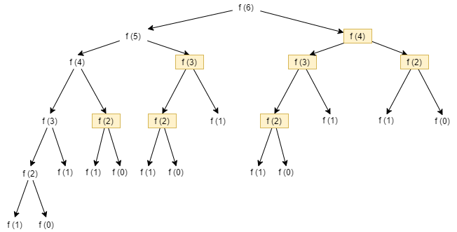
If we analyze the computation required for the 6th Fibonacci number in both the iterative and recursive algorithms, the truth becomes evident. The recursive algorithm calculates the 5th Fibonacci number by recursively calling FIB(4) and FIB(3). In turn, FIB(4) calls FIB(3) and FIB(2). Notice that FIB(3) is actually calculated twice! This is a problem. If we calculate the 36th Fibonacci number, the values of many Fibonacci numbers are calculated repeatedly, over and over.

Tracing the Program

To clarify our ideas further, we can consider the recursive tree resulting from the trace of the program to calculate the 6th Fibonacci number. Each of the computations highlighted in the diagram will have been computed previously.

If we count the recomputations, we can see how we calculate the 4th Fibonacci number twice, the 3rd Fibonacci number three times, and the 2nd Fibonacci five times. All of this is due to the fact the we do not consider the work done by other recursive calls. Furthermore, the higher our initial number, the worse the situation grows, and at a very rapid pace.

Memoization

To avoid recomputing the same Fibonacci number multiple times, we can save the results of various calculations and reuse them directly instead of recomputing them. This technique is called memoization, which can be used to optimize some functions that use tree recursion.

To implement memoization, we simply store the values the first time we compute them in an array. The following pseudocode shows an efficient algorithm that uses an array, called FA, to store and reuse Fibonacci numbers.

function FIBOPT(N)
    if N == 0
        return 0
    else if N == 1
        return 1
    else if FA[N] == -1
        FA[N] = FIBOPT(N-1) + FIBOPT(N-2)
        return FA[N]
    else
        return FA[N]
    end if
end function

We assume that each element in FA has been initialized to -1. We also assume that N is greater than 0 and that the length of FA is larger than the Fibonacci number N that we are trying to compute. (Of course, we would normally put these assumptions in our precondition; however, since we are focusing on the recursive nature of the function, we will not explicitly show this for now.) The cases where N == 0 and N == 1 are the same as we saw in our previous FIB function. There is no need to store these values in the array when we can return them directly, since storing them in the array takes additional time. The interesting cases are the last two. First, we check to see if FA[N] == -1, which would indicate that we have not computed the Fibonacci number for N yet. If we have not yet computed N’s Fibonacci number, we recursively call FIBOPT(N-1) and FIBOPT(N-2) to compute its value and then store it in the array and return it. If, however, we have already computed the Fibonacci for N (i.e., if FA[N] is not equal to -1), then we simply return the value stored in the array, FA[N].

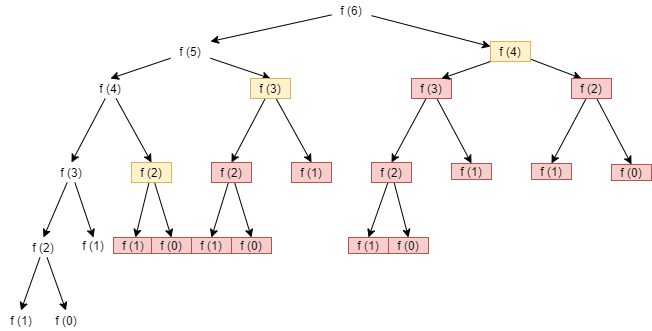
As shown in our original call tree below, using the FIBOPT function, none of the function calls in red will be made at all. While the function calls in yellow will be made, they will simply return a precomputed value from the FA array. Notice that for N = 6, we save 14 of the original 25 function calls required for the FIB function, or a $56\%$ savings. As N increases, the savings grow even more.