Merge Sort Time Complexity
Now that we’ve reviewed the pseudocode for the merge sort algorithm, let’s see if we can analyze the time it takes to complete. Analyzing a recursive algorithm requires quite a bit of math and understanding to do it properly, but we can get a pretty close answer using a bit of intuition about what it does.
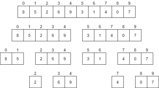
For starters, let’s consider a diagram that shows all of the different recursive calls made by merge sort, as shown below.
The first thing we should do is consider the worst-case input for merge sort. What would that look like? Put another way, would the values or the ordering of those values change anything about how merge sort operates?
The only real impact that the input would have is on the number of swaps made by merge sort. If we had an input that caused each of the base cases with exactly two elements to swap them, that would be a few more steps than any other input. Consider the highlighted entries below.
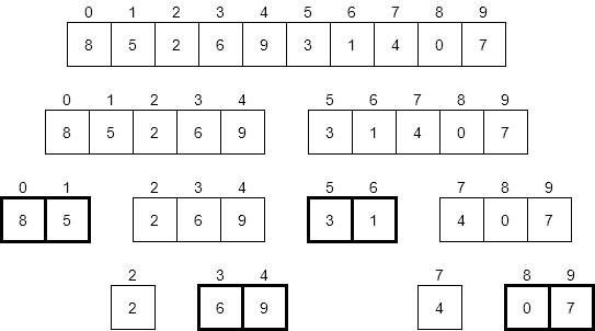
If each of those pairs were reversed, we’d end up doing that many swaps. So, how many swaps would that be? As it turns out, a good estimate would be $N / 2$ times. If we have an array with exactly 16 elements, there are at most 8 swaps we could make. With 10 elements, we can make at most 4. So, the number of swaps is on the order of N time complexity.
What about the merge operation? How many steps does that take? This is a bit trickier to answer, but let’s look at each row of the diagram above. Across all of the calls to merge sort on each row, we’ll end up merging all $N$ elements in the original array at least once. Therefore, we know that it would take around $N$ steps for each row in the diagram. We’ll just need to figure out how many rows there are.
A better way to phrase that question might be “how many times can we recursively divide an array of $N$ elements in half?” As it turns out, the answer to that question lies in the use of the logarithm.
Logarithm
The logarithm is the inverse of exponentiation. For example, we could have the exponentiation formula:
$$ \text{base}^{\text{exponent}} = \text{power} $$
The inverse of that would be the logarithm $$ \text{log}_{\text{base}}(\text{power}) = \text{exponent} $$
So, if we know a value and base, we can determine the exponent required to raise that base to the given value.
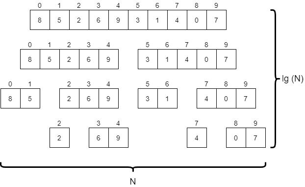
In this case, we would need to use the logarithm with base $2$, since we are dividing the array in half each time. So, we would say that the number of rows in that diagram, or the number of levels in our tree would be on the order of $\text{log}_2(N)$. In computer science, we typically write $\text{log}_2$ as $\text{lg}$, so we’ll say it is on the order of $\text{lg}(N)$.
To get an idea of how that works, consider the case where the array contains exactly $16$ elements. In that case, the value $\text{lg}(16)$ is $4$, since $2^4 = 16$. If we use the diagram above as a model, we can draw a similar diagram for an array containing $16$ elements and find that it indeed has $4$ levels.
If we double the size of the array, we’ll now have $32$ elements. However, even by doubling the size of the array, the value of $\text{lg}(32)$ is just $5$, so it has only increased by $1$. In fact, each time we double the size of the array, the value of $\text{lg}(N)$ will only go up by $1$.
With that in mind, we can say that the merge operation runs on the order of $N * \text{lg}(N)$ time. That is because there are ${\text{lg}(N)}$ levels in the tree, and each level of the tree performs $N$ operations to merge various parts of the array together. The diagram below gives a good graphical representation of how we can come to that conclusion.
Putting it all together, we have $N/2$ swaps, and $N * \text{lg}(N)$ steps for the merge. Since the value $N * \text{lg}(N)$ is larger than $N$, we would say that total running time of merge sort is on the order of $N * \text{lg}(N)$.
Later on in this chapter we’ll discuss how that compares to the running time of selection sort and bubble sort and how that impacts our programs.