Performance of Sorting Algorithms
We introduced four sorting algorithms in this chapter: selection sort, bubble sort, merge sort, and quicksort. In addition, we performed a basic analysis of the time complexity of each algorithm. In this section, we’ll revisit that topic and compare sorting algorithms based on their performance, helping us understand what algorithm to choose based on the situation.
Overall Comparison
The list below shows the overall result of our time complexity analysis for each algorithm.
- Selection Sort: $N^2$
- Bubble Sort: $N^2$
- Merge Sort: $N * \text{lg}(N)$
- Quicksort Average Case: $N * \text{lg}(N)$
- Quicksort Worst Case: $N^2$
We have expressed the amount of time each algorithm takes to complete in terms of the size of the original input $N$. But how does $N^2$ compare to $N * \text{lg}(N)$?
One of the easiest ways to compare two functions is to graph them, just like we’ve learned to do in our math classes. The diagram below shows a graph containing the functions $N$, $N^2$, and $N * \text{lg}(N)$.
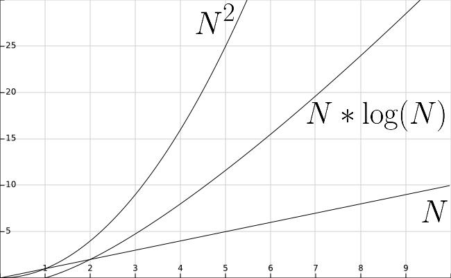
First, notice that the scale along the X axis (representing values of $N$) goes from 0 to 10, while the Y axis (representing the function outputs) goes from 0 to 30. This graph has been adjusted a bit to better show the relationship between these functions, but in actuality they have a much steeper slope than is shown here.
As we can see, the value of $N^2$ at any particular place on the X axis is almost always larger than $N * \text{lg}(N)$, while that function’s output is almost always larger than $N$ itself. We can infer from this that functions which run in the order of $N^2$ time will take much longer to complete than functions which run in the order of $N * \text{lg}(N)$ time. Likewise, the functions which run in the order of $N * \text{lg}(N)$ time themselves are much slower than functions which run in linear time, or in the order of $N$ time.
Based on that assessment alone, we might conclude that we should always use merge sort! It is guaranteed to run in $N * \text{lg}(N)$ time, with no troublesome worst-case scenarios to consider, right? Unfortunately, as with many things in the real world, it isn’t that simple.
Choosing Sorting Algorithms
The choice of which sorting algorithm to use in our programs largely comes down to what we know about the data we have, and how that information can impact the performance of the algorithm. This is true for many other algorithms we will write in this class. Many times there are multiple methods to perform a task, such as sorting, and the choice of which method we use largely depends on what we expect our input data to be.
For example, consider the case where our input data is nearly sorted. In that instance, most of the items are in the correct order, but a few of them, maybe less than $10%$, are slightly out of order. In that case, what if we used a version of bubble sort that was optimized to stop sorting as soon as it makes a pass through the array without swapping any elements? Since only a few elements are out of order, it may only take a few passes with bubble sort to get them back in the correct places. So even though bubble sort runs in $N^2$ time, the actual time may be much quicker.
Likewise, if we know that our data is random and uniformly distributed, we might want to choose quicksort. Even though quicksort has very slow performance in the worst case, if our data is properly random and distributed, research shows that it will have better real-world performance than most other sorting algorithms in that instance.
Finally, what if we know nothing about our input data? In that case, we might want to choose merge sort as the safe bet. It is guaranteed to be no worse than $N * \text{lg}(N)$ time, even if the input is truly bad. While it might not be as fast as quicksort if the input is random, it won’t run the risk of being slow, either.